| Issue |
A&A
Volume 706, February 2026
|
|
|---|---|---|
| Article Number | A108 | |
| Number of page(s) | 15 | |
| Section | Interstellar and circumstellar matter | |
| DOI | https://doi.org/10.1051/0004-6361/202556132 | |
| Published online | 10 February 2026 | |
Glycolaldehyde and ethanol toward the L1157 outflow: Resolved images and constraints on glycolaldehyde formation
1
Univ. Grenoble Alpes, CNRS, IPAG,
38000
Grenoble,
France
2
Institut de Radioastronomie Millimétrique,
38406
Saint-Martin d’Hères,
France
3
INAF, Osservatorio Astrofisico di Arcetri,
Largo E. Fermi 5,
50125
Firenze,
Italy
★ Corresponding author: This email address is being protected from spambots. You need JavaScript enabled to view it.
Received:
27
June
2025
Accepted:
16
October
2025
Abstract
Context. Interstellar complex organic molecules, also known as iCOMs, are species of special interest in astrochemistry because of their potential role in the emergence of life. The discovery of iCOMs in the interstellar medium has sparked a decades-long debate about how they are formed. In principle, two main routes are possible: on the surfaces of dust grains and in the gas phase. A powerful way to discriminate between and constrain the two routes is to observe iCOMs along protostellar outflow-shocked regions, provided their ages are well constrained. In this way, the chemical evolution over time can be probed.
Aims. We focused on glycolaldehyde (CH2OHCHO) and ethanol (C2H5OH), and their possible daughter-mother relationship, as suggested by previous studies. More precisely, our objective was to verify whether the gas-phase reactions derived in these studies dominate the formation of glycolaldehyde, so whether this gas-phase formation pathway can account for the abundance of glycolaldehyde observed in star-forming regions. We targeted the well-known southern outflow of L1157, which hosts three shocked regions, B0, B1 and B2, of increasing ages: approximately 900, 1500 and 2300 years, respectively.
Methods. We obtained high-resolution (∼4″) IRAM NOEMA maps of three glycolaldehyde lines and one ethanol line toward the entire southern outflow lobe of L1157 and used them to derive the abundances of the two species in B0, B1 and B2, as well as their abundance ratio. We then used a pseudo time-dependent astrochemical code to model the post-shock gas-phase chemistry of the two molecules under study, in which glycolaldehyde is formed via gas-phase reactions starting from ethanol, via the so-called ethanol-tree scheme, or on the grain surfaces. On the contrary, ethanol is assumed to be form on grain surfaces and to be released into the gas phase by the passage of the shocks. Once in the gas, C2H5OH is gradually consumed to form, among other iCOMs, glycolaldehyde. Ethanol is mainly destroyed through reactions with the OH radical, which in turn is primarily formed by injected (previously frozen) water (H2O).
Results. We present the first spatially resolved maps of ethanol and glycolaldehyde toward the L1157 southern outflow and, more generally, toward solar-like star-forming regions. From these maps, we computed their column densities in B0, B1 and B2. Assuming an excitation temperature of 30 K for both species, we find column densities ranging between 1 and 3 ×1013 cm−2 for glycolaldehyde and between 4 and 6 ×10¹³ for ethanol. Their relative abundance ratio [CH2OHCHO] / [C2H5OH], equal to 0.25-0.4, increases between B1 and B2. The measured abundance ratios in B1 and B2 are relatively well reproduced by the astrochemical model. However, our model cannot simultaneously reproduce the observations toward B0, and toward B1 and B2, whether we assume that glycolaldehyde is primarily formed in the gas phase or on the grain-surfaces. This likely indicates that one of the assumptions in our model is incorrect. Possible candidates include the excitation temperature and grain mantle composition, assumed to be the same in B0, B1 and B2; the age of B0; and the gas temperature, assumed to be constant after the shock passage. Nonetheless, our modeling rules out the possibility that all the observed gaseous glycolaldehyde is a grain-surface product.
Conclusions. The study of resolved iCOM emission in the direction of protostellar molecular outflows proves to be an efficient way to constrain their formation routes. In the future, it will be important to carry out similar studies in regions other than L1157 outflow. In addition, improved modeling of shock chemistry should be developed, in which physical properties vary with time along with chemistry.
Key words: ISM: abundances / ISM: jets and outflows / ISM: individual objects: L1157
This work is based on observations carried out under project number I17AB with the IRAM NOEMA Interferometer. IRAM is supported by INSU/CNRS (France), MPG (Germany) and IGN (Spain).
© The Authors 2026
 Open Access article, published by EDP Sciences, under the terms of the Creative Commons Attribution License (https://creativecommons.org/licenses/by/4.0), which permits unrestricted use, distribution, and reproduction in any medium, provided the original work is properly cited.
This article is published in open access under the Subscribe to Open model. This email address is being protected from spambots. You need JavaScript enabled to view it. to support open access publication.
1 Introduction
Among the more than 330 molecules detected in the interstellar medium (ISM)1, those with more than six atoms and containing carbon plus at least one other heavy atom are of particular interest due to their potential impact on the emergence of life on Earth and other planets. These molecules are referred to as interstellar complex organic molecules (iCOMs; Ceccarelli et al. 2017; Herbst & van Dishoeck 2009). Glycolaldehyde (CH2OHCHO; hereafter GA), is a particularly interesting iCOM due to its prebiotic potential being simplest sugar, that can lead to the formation of more complex sugars such as ribose, a key component of ribonucleic acid (RNA; Weber 1998; Jalbout et al. 2007).
GA was first detected toward the massive star-forming region Sagittarius B2(N) by Hollis et al. (2000) (see also Hollis et al. 2004; Halfen et al. 2006). Subsequently, Beltrán et al. (2009) reported the detection of GA toward the massive hot core G31.41+0.31, marking the first detection of this molecule outside of the Galactic Center. CH2OHCHO has since been detected in other star-forming regions, notably toward the solarlike protostars IRAS 16293-2422 (Jørgensen et al. 2012, 2016), NGC1333 IRAS2A, IRAS4A, IRAS4B1 and SVS13A (Coutens et al. 2015; Taquet et al. 2015; De Simone et al. 2017). Finally, CH2OHCHOwas detected in the protostellar shocked region B1 of the L1157 molecular outflow by Lefloch et al. (2017), using single-dish observations as part of the IRAM2 Large Program ASAI (Astrochemical Surveys At IRAM: Lefloch et al. 2018).
Despite these detections in various sources, the formation route of GA, as for other iCOMs, remains hotly debated. In general, two possible iCOM formation pathways are evoked in the literature (e.g. Ceccarelli 2023; Ceccarelli et al. 2023): reactions occurring on dust grain-surfaces (Garrod et al. 2006, 2008) or in the gas phase (e.g. Vasyunin & Herbst 2013; Balucani et al. 2015).
Discriminating which of the two routes operate for different iCOMs is challenging and astronomical observations have previously provided some constraints (e.g. Codella et al. 2017, 2020; López-Sepulcre et al. 2024; Balucani et al. 2024).
For GA, Lefloch et al. (2017) found a good correlation between the abundances of ethanol (C2H5OH) and GA in their observations of L1157-B1, together with three hot corinos: NGC 1333 IRAS 4A and IRAS 2A (Taquet et al. 2015) and IRAS 16293-2422 (Jørgensen et al. (2016); Jaber et al. (2014). Inspired by study of the Lefloch et al. (2017), Skouteris et al. (2018) propose a scheme to form GA in the gas phase, via a two-step chain of reactions starting from ethanol, known as the “ethanol genealogical tree”. Their theoretical predictions, obtained from quantum mechanics (QM) calculations, agree closely with the observed GA and ethanol abundances toward the hot corinos mentioned above. Specifically, the GA/ethanol abundance ratios in these sources are consistent with the theoretically derived branching ratio, which holds only in steady-state conditions (valid for the high density in the hot corinos: e.g., Ceccarelli et al. 1996; Taquet et al. 2014).
A much stronger test can be performed by adding the time constraint. This can be achieved by imaging the emission of the two species in distinct shocked regions of a molecular outflow, produced by shocks from subsequent ejection events. This method has already proven to be successful in constraining the formation route of formamide (NH2CHO), for example (Codella et al. 2017; López-Sepulcre et al. 2024). In this article, we use the same approach to constrain the formation route of GA. To this end, we present the first ever resolved images of GA and ethanol line emission toward the molecular outflow emanating from L1157-mms, and we compare our observations with theoretical time-dependent predictions of their abundances.
The article is organized as follows. Sect. 2 provides an overview of the target; Sect. 3 describes the observations; Sect. 4 presents the observational results and derives the column densities and abundances of GA and ethanol along the outflow; Sect. 5 describes the astrochemical model and the obtained predictions; in Sect. 6 discusses the implications of the comparison between observations and model predictions; and Sect. 7 summarizes the key findings of the present work.
2 L1157 southern outflow
L1157-mms (Tobin et al. 2022) is a Class 0 protobinary system that drives at least one episodic and precessing jet (Gueth et al. 1996; Podio et al. 2016). It is located in the Cepheus molecular cloud system at a distance of 352 ± 18 pc (Zucker et al. 2019) and has a systemic velocity of +2.6 km s−1 (Bachiller & Pérez-Gutiérrez 1997). The L1157 southern outflow lobe, which is blueshifted, extends over a projected length of ~0.2 pc (PAoutflow ~ −17°, see Podio et al. 2016). This outflow lobe has been the subject of numerous molecular studies, e.g Tafalla & Bachiller 1995; Gueth et al. 1996; Arce et al. 2008; Lefloch et al. 2017; Podio et al. 2016; Codella et al. 2017; López-Sepulcre et al. 2024, and is known for its richness in iCOMs, making it a perfect target for studying their formation. The associated jet, whose velocity has been estimated to be ~90 km s−1 in the southern region, created three shocked regions toward the south, B0, B1 and B2, each of them fragmented into several clumps (Benedettini et al. 2007, see Fig. 1).
Previous studies have revealed that shocked regions are particularly enriched in various molecular species. In particular, strong line emission from SiO and methanol has been detected toward L1157-B1 (Mikami et al. 1992; Bachiller & Pérez-Gutiérrez 1997), along with other less abundant species, such as CN, SO, SO2, H2CO, C2H5OH, CH3CHO, HCOOCH3, CH3OCH3, t-HCOOH, NH2CHO, HNCO and CH3CN (see Bachiller & Pérez-Gutiérrez 1997; Codella et al. 2009; Mendoza et al. 2014; Lefloch et al. 2017; López-Sepulcre et al. 2024), whose abundances are enhanced by up to a few orders of magnitude compared with quiescent molecular gas. This behavior is explained by the drastic change in physical conditions caused by the shock itself, which releases species that were previously trapped in the icy mantles and refractory cores of dust grains into the gas phase (Bachiller et al. 1995; Bachiller & Pérez-Gutiérrez 1997), by sputtering or shattering of the grains. Once in the gas, these species can react to form new molecules. In addition, B0, B1 and B2 have different ages, which are relatively well constrained and range between ~900 yr and ~2500 yr (Podio et al. 2016), as summarized in Table 2.
The blueshifted outflow of L1157 is therefore an ideal and unique target for testing the predictions of astrochemical models in terms of the evolution of molecular abundances evolution with time.
3 Observations
The southern outflow of the L1157 protobinary was observed at 3 mm with the IRAM NOrthern Extended Millimeter Array (NOEMA) in December 2017, January 2018 and May 2018, for a total of 21 hours in configuration D (the most compact configuration), using nine antennas. These observations were made using a mosaic of eight fields that covered a total area of approximately 2.5 arcsec2. The shortest and longest projected baselines were 24.0 m and 176.0 m, respectively, which allowed us to recover emission at scales from ~3.5″ up to ~26″ at 3 mm. The smallest angular scale corresponds to ~1230 au on the source. The phase center is α(J2000) = 20h39m09s.635, δ(J2000) = +68°01′19″.80. We used the PolyFix correlator, covering the frequency ranges 81.5-89.2 GHz and 96.9-104.6 GHz. The molecular lines analyzed in this work were observed with a spectral resolution of 2 MHz (corresponding to ~7 km s−1 at 85 GHz).
The system temperature varied between 80 and 300 K during most of the tracks, and the amount of precipitable water vapor ranged between 2.5 and 5.5 mm. 3C454.3, 3C84, 3C273, 1928+738 and 2013+370 were used as bandpass calibrators, and the absolute flux scale was fixed by observing MWC349 and LKHA101. The calibration of the gains in phase and amplitude was made on 2010+723, 1928+738 and J1933+656. The estimated uncertainty on the calibrated absolute flux scale is ≤10%.
The data were calibrated using the CLIC software from the GILDAS package3. We also used the MAPPING software from the GILDAS package to perform imaging and deconvolution, using a natural weighting to maximize sensitivity. The continuum emission, originating exclusively from the protobinary L1157-mms, was subtracted in the visibility plane. The synthesized beam sizes and 1σ root mean square (RMS) achieved are summarized in Tables 1 and 2 respectively.
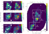 |
Fig. 1 Zoom on the three shocked regions. The left panel shows a zoom on the GA and ethanol emission maps toward B0, B1, and B2, integrated over the velocity range [−10,5] km s−1. The velocity-integrated emission is shown by white and red contours for the GA and ethanol lines, respectively, overlaid on the emission of the CH3OH line 51,5−40,4 in color scale. For the GA and ethanol lines, the first contours are drawn at 3σ and the subsequent contours are plotted in steps of 1σ (1σ = 15 mJy/beam km/s for CH2OHCHO and 12 mJy/beam km/s for C2H5OH in B0 and B1; 18 mJy/beam km/s for CH2OHCHO and 14 mJy/beam km/s for C2H5OH in B2). The ellipses in the corners indicate the synthesized beams for each GA and ethanol line. The white triangles and associated labels mark the different clumps identified by Benedettini et al. (2007). The right panel shows the velocity-integrated intensity map of the CH3OH 51,5−40,4 line, illustrating the morphology of the overall L1157 southern molecular outflow. The methanol map was used to define the polygons (shown by magenta contours) within which the intensities used for the column density computations are integrated (see text). The methanol map is centered at α(J2000) = 20h39m09.635s and δ(J2000) = 68°01′19.80″. The first contour is drawn at 50σ and subsequent contours are plotted in steps of 100σ (1σ = 11 mJy/beam km/s). The black ellipse in the bottom right corner indicates the synthesized beam of the CH3OH line. The white squares centered on B0, B1 and B2 delimit the areas of the zoomed maps shown in the left panels. The white star at the top of the map marks the position of the unresolved L1157 protobinary system (Tobin et al. 2013, 2022). |
4 Results
We detected one ethanol and three GA lines, whose Eup values range between ~18 K and 28 K. We carefully verified that none of the four lines is affected by possible blending with another species. For example, we excluded the GA transition at f = 102 549.78 MHz, because of the possible line blending with a methyl acetylene (CH3CCH) transition. The detection of the four lines confirms the previous detections obtained with the 30m IRAM single-dish telescope toward B1 by Lefloch et al. (2017). The spectral parameters of the detected lines are reported in Table 1.
We imaged the emission of the four detected lines and, in addition, one methanol (CH3OH) line (transition 51,5−40,4 E) with Eup = 40.4 K and an Einstein coefficient Aij = 1.9 × 10⁻⁶ s−1 (see Table 1), for visualization and analysis purposes (see below).
Spectral parameters of the detected molecular lines.
Derived properties of the detected line emission in the different shocked regions.
4.1 Maps and Integrated line intensities
The left panels of Figure 1 present the GA and ethanol maps toward B0, B1 and B2, respectively, while the right panel shows the methanol map, which provides the overall outflow morphology. Although GA and ethanol have already been detected toward B1 with the IRAM 30-m telescope (Lefloch et al. 2017), this is the first time that a resolved map of these two species has been obtained in a solar-type star-forming region.
The GA transition 101,10−90,9, shown in Fig. 1, is the brightest of the three GA lines identified in our data (S/N ~ 6). We detected GA emission in a few clumps toward B0, B1 and B2, with the overall brightest emitting regions in B2. We emphasize that because it is a mosaic, there are more noise fluctuations at the edges than in the center of the maps, resulting in higher noise in B2. Ethanol emission is also seen in clumps toward B0, but it is more extended toward B1 and B2. Overall, the ethanol line shows comparable intensity in all three shocked regions.
We estimated the GA and ethanol line intensity recovered by the interferometer toward B1 using the ASAI survey obtained with the IRAM 30m single-dish telescope. We found that we recover 100% of the line flux for each transition (see Appendix B for details).
To compute the molecular column densities toward B0, B1 and B2, we defined polygons based on the methanol line image, as shown by the magenta contours in the right panel of Fig. 1.
In the following, we describe the maps at B0, B1 and B2 in detail, and the chosen polygons. Table 2 summarizes the line intensities integrated over the polygons and velocity. For each line, we integrated the flux over the channels where emission exceeds 3σ RMS and, to maintain consistency, adopted the same velocity range for all detected lines.
4.1.1 B0 region
The emission of both ethanol and GA is located in the northern part of B0, roughly around the same clumps, B0c and B0d. Their spatial distributions match that of methanol closely; in particular, the three clumps where CH2OHCHO and C2H5OH emission is enhanced are also bright in CH3OH (Fig. 1; B0 a, c and d). Therefore, we chose the polygon that encompasses the three spots B0 a, c and d.
In B0, we could only detect two GA transitions with a signal-to-noise ratio (S/N) greater than 3: 80,8−71,7 and 101,10−90,9.
4.1.2 B1 region
In B1, GA emission is weak and distributed mainly to the north of the region. Ethanol, on the other hand, is relatively bright and extended mostly toward the west, just below the northernmost GA emission. As in B0, we could detect only two GA transitions, with the 81,8−70,7 transition having a S/N ≤ 3 in this region.
Around B1, we defined a polygon that encompasses the brightest methanol emission. We note that extending the polygon to include the northern GA clump emission would result in a signal that is too diluted relative to the noise.
Column densities and abundance ratios.
4.1.3 B2 region
The B2 region is where the GA emission is the brightest within the entire L1157 southern outflow. In this region, there is a slight spatial segregation between GA and ethanol: ethanol appears to be more prominent in the north of B2a, whereas GA is located slightly toward the south compared with ethanol.
The polygon used for B2 encompasses the brightest area around B2a in the methanol emission. We excluded the area around B2b because the noise RMS is significantly higher, as it is located at the edge of the mosaic.
4.2 Column densities and molecular abundance ratios
We derived the column densities from the velocity-integrated intensities of GA and ethanol lines5. To this end, we assumed that the emission is at local thermal equilibrium (LTE), that all lines are optically thin6 and that GA and ethanol lines trace the same gas (as discussed in Lefloch et al. 2017). A non-LTE analysis could not be carried out owing to the lack of collisional coefficients.
When applying the LTE method, we find that the GA 81,8−70,7 line (at 85.782 GHz) intensity is systematically too low to fit with the other two GA lines. Since the NOEMA integrated interferometric and ASAI data toward B1 agree very well, this implies that the low 81,8−70,7 line intensity is not due to a problem with the NOEMA observations, but that it may be due to a non-LTE effect that we cannot reproduce with our analysis. For example, in B1, assuming a GA column density of (1.3 ± 0.2) × 1013 cm−2 for a Tex = 30 K (see below), LTE analysis predicts an integrated intensity of 0.12 ± 0.02 K km s1 for the 81,8−70,7 transition, which is twice as large as the measured value. Therefore, in the following, we use only the other two GA lines.
We attempted to estimate an excitation temperature, Tex, with the two GA lines but, given the relatively large error bars on their intensities, we could only derive a lower limit to Tex at each position, as listed in Table 3. Since Lefloch et al. (2017) found Tex=30 ± 5 K in B1 using 14 GA lines, we computed the column density, Nga, at 30 K in the three regions as a reference value. However, we also computed Nga in the three regions varying Tex from 10 to 100 K, to evaluate the impact of the choice of Tex. The results are shown in Fig. 2. Assuming the same excitation temperature for all three regions, we observe that Nga is similar in B0 and B1 and significantly higher in B2. However, the three temperatures could actually differ, with B0 being warmer than B1 and B2 (López-Sepulcre et al. 2024).
Using the literature value for the H-nuclei column density in B1, Nh=2 × 1021 cm−2 (Lefloch et al. 2012), we estimated the GA abundance. We assumed that NH is the same in B0, B1 and B2, based on the CO (J=1-0) emission map of Gueth et al. (1996). In the literature, NH is reported to range between (1-4) × 1021 cm−2 for B1 (Bachiller & Pérez-Gutiérrez 1997; Lefloch et al. 2012; Mendoza et al. 2014; Codella et al. 2017), while no estimates are available for B0 and B2. Thus, we computed the uncertainties in the absolute abundances by accounting for a factor-of-two uncertainty on NH.
Finally, we derived the GA/ethanol abundance ratio, considering the ratio between the column densities of each species obtained using the same Tex, which was varied between between 10 and 100 K. Figure 2 shows the dependence of the GA/ethanol abundance ratio on Tex and Table 3 lists representative values. Again, assuming the same temperature in each region, the ratio is larger in B2 than in B0 and B1. The ratio varies by a factor of approximately three at each position across the excitation temperature values considered, i.e., between 10 K and 100 K. To compare the astrochemical model predictions with observations, we assumed that the three regions (B0, B1 and B2) have the same Tex and explored three temperatures: 15, 30 and 50 K.
The errors in the column densities account for the noise RMS plus a 10% uncertainty on the absolute intensity scale; the errors in the absolute abundances include an additional factor of two due to the uncertainty in the H-nuclei column densities; the abundance ratios do not include either the calibration or the Nh uncertainty.
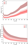 |
Fig. 2 Glycolaldehyde (GA) column density and abundance ratio, computed from the 101,10−90,9 line, which is the brightest, assuming LTE population and optically thin line emission. The bands represent the uncertainty associated with the line intensity (see text). Upper panel: column density of GA in B0 (light pink), B1 (pink) and B2 (dark pink), as a function of the excitation temperature Tex. The column density values partially overlap in B0 and B1. Lower panel: GA/ethanol abundance ratio versus Texc in B0, B1 and B2 (same color coding as above). |
5 Chemical modeling
We compared the measured abundances with those predicted by the pseudo-time-dependent astrochemical model described in Section 5.1. Given the uncertainty in the absolute abundance derivation (see discussion in Section 4.2), we primarily considered the ratio between GA and ethanol abundances, summarized in Table 2, rather than the absolute abundances themselves. In the astrochemical model, we used the most up-to-date chemical reaction network for the formation and destruction of GA and ethanol in the gas phase, summarized in Section 5.2.
5.1 Model description
We followed the same method as in previous studies by our group (e.g., Podio et al. 2014; Codella et al. 2017, 2020; Tinacci et al. 2023; Giani et al. 2023; López-Sepulcre et al. 2024), using the GRAINOBLE code (Taquet et al. 2012; Ceccarelli et al. 2018) with the gas-phase-only option, and the gas-phase reaction network described in the next section.
Briefly, the passage of a shock is characterized by a sudden increase in the shocked gas density and temperature, and by the partial release into the gas phase of the components of the dust icy mantles and refractory cores. This release is caused by the sputtering (gas-grain collisions) and shattering (grain-grain collisions) of grains which, depending on the velocity of the shock, can liberate species from the dust icy mantles and fragment their refractory cores. (e.g., Flower et al. 1996; Field et al. 1997; Caselli et al. 1997; Jiménez-Serra et al. 2008; Gusdorf et al. 2008).
Accordingly, in our model, we increase the shocked gas density and temperature as well as the gaseous abundances of species known to be components of icy dust mantles and refractory grain cores. The model consists of two stages that simulate the gas conditions before and after the shock passage, as follows.
Stage 1. We derived the steady-state gas-phase abundances of a typical molecular cloud with a temperature Tgas = 10 K and an H-nuclei density nH = 2×104 cm−3. These abundances represent the gas chemical composition before the passage of the shock and are used as input for the Stage 2 modeling.
Stage 2. We set the density and temperature of the gas to the values previously derived for the post-shocked gas in L1157-B1, Tgas = 90 K and H-nuclei density nH = 8×105 cm−3 (e.g., Lefloch et al. 2012; Codella et al. 2017). We also increase the abundances of the species injected into the gas phase due to the shock passage, again based on previous determinations of the abundances listed in Table 4. Finally, we follow the abundance of the various species as a function of time.
5.2 Chemical network: Formation and destruction of glycolaldehyde and ethanol
We used the GRETOBAPE-gas reaction network described in Tinacci et al. (2023), updated according to more recent works by Giani et al. (2023), Giani et al. (2025) and Balucani et al. (2024).
Below, we review the reactions involved in the formation and destruction of GA and ethanol, the two target species of this work.
Glycolaldehyde. Until recently, no gas-phase formation routes for GA were known that could explain its observed abundance in the interstellar medium. For instance, Halfen et al. (2006) proposed that a sequence of gas-phase reactions, triggered by gaseous formaldehyde (H2CO) reacting with its protonated form (H2COH+), could lead to the synthesis of GA. However, later modeling by Woods et al. (2012) showed that this route is inefficient at the ISM temperatures. Meanwhile, given the difficulty of identifying gas-phase reactions responsible for the formation of several other iCOMs (e.g., see the discussion in Garrod et al. 2006; Ceccarelli et al. 2023), the astrochemical community focused its attention on the possibility that GA forms on the cold dust grain surfaces during the prestellar phase (e.g. Garrod et al. 2006). In the case of GA, Garrod et al. (2008) proposed that it forms via the association of HCO with CH2OH. However, subsequent quantum chemistry computations by Enrique-Romero et al. (2022) showed that the HCO + CH2OH reaction on icy surfaces (as in the ISM) has a barrier of ~1.7 kJ/mol (equivalent to ~200 K) and, more importantly, competes with H abstraction from HCO to form CO + CH3OH, a reaction without an activation barrier, making it more probable than GA formation. Thus, the formation of GA via this grain-surface route is likely inefficient.
Based on the observed correlation between ethanol and GA (Lefloch et al. 2017), Skouteris et al. (2018) propose an alternative way to form GA in the gas phase, starting from gaseous ethanol (see below for its formation), which they term the “ethanol tree”. Briefly, in this scheme, ethanol reacts with OH (and Cl) to form the CH3CHOH and CH2CH2OH radicals. The subsequent reaction of both radicals with O leads to the formation of formic acid (HCOOH), acetic acid (CH3COOH) and acetaldehyde (CH3CHO) from CH3CHOH, and formaldehyde (H2CO) and GA from CH2CH2OH. Skouteris et al. (2018) also performed quantum chemistry calculations and provides the formation rate of all the products and their branching fraction. The reaction forming GA shows a weak dependence on temperature (∝ T0.16: Skouteris et al. 2018).
Finally, gaseous GA is mainly destroyed by reactions with abundant molecular ions (HCO+, H3O+, H+3).
In the present work, we focus primarily on the gas-phase formation route of GA, namely the ethanol tree scheme of Skouteris et al. (2018). Our goal was to verify whether this mechanism can reproduce the observed GA abundance or whether additional routes forming GA on the grain surfaces are absolutely necessary. We emphasize that we do not provide any specific constraints on the grain-surface routes for the following reason. The possible amount of GA formed on the grain surfaces is entirely model dependent because our observations are sensitive only to how much GA is injected into the gas phase, not how it was formed. Nonetheless, we also tested the possibility that GA originates entirely from grain-surface formation and is subsequently injected into the gas phase.
Ethanol. Efficient gas-phase reactions for the formation of ethanol are not known; thus, it is believed to form on dust grain surfaces, as it is the case for many saturated molecules such as methanol (e.g. Tielens & Hagen 1982; Hama & Watanabe 2013; Rimola et al. 2014).
Garrod et al. (2008) proposed that ethanol is formed by the combination of the radicals CH2OH and CH3, similar to the formation route proposed by the same authors for GA (discussed above). Again, quantum chemistry calculations by Enrique-Romero et al. (2022) show that the CH2OH + CH3 reaction has an activation barrier of 2.5 kJ/mol (=300 K) and competes with the formation of CH4 + H2CO. Subsequently, Garrod et al. (2022) propose that ethanol is formed by the combination of CH3CH2 with O on the grain surfaces, a reaction competing with the hydrogenation of the former. In the same year, Perrero et al. (2022) put forward that ethanol can be formed by the reaction of CCH, landing from the gas phase onto the iced grain surface, with a molecule of water ice enveloping the dust grains, followed by hydrogenation. Finally, Ferrero et al. (2024) show that an alternative route for ethanol formation, efficient in the early phases, involves the reaction of C atoms landing on the ice grain surfaces forming COH2, followed by a barrierless reaction with CH3 and subsequent hydrogenation. In summary, at least four ethanol formation routes on grain surfaces have been proposed in the literature.
Once injected into the gas phase by the shock passage, ethanol is destroyed by reactions involving abundant molecular ions, especially H3O+, as in the case of GA above, as well as by reactions with OH, which is also the first step toward the formation of GA (see above and Skouteris et al. 2018). The ethanol destruction reactions and their rate coefficients are summarized in Table 5.
Reaction (1), C2H5 OH + OH : we adopted the rate constants reported by Skouteris et al. (2018), based on laboratory measurements by Caravan et al. (2015) in the 293-54 K range. This reaction represents the first step of the “ethanol tree” leading to GA formation.
Reaction (2), C2H5 OH + H3O+: we adopted the rate constants from the KIDA database7. However, that the most recent UMIST8, based on old laboratory measurements by Bohme et al. (1979), later confirmed by Spanel & Smith (1997) database release reports rate constants larger by a factor 1.6. The dependence of the rate constant as a function of the temperature is assumed to follow the classical Su-Chesnavich model, i.e. k ∝ T−0.5. More recent and sophisticated treatments for the temperature dependence have since been developed: the adiabatic capture centrifugal sudden approximation (ACCSA) by Clary (1985) and the statistical adiabatic channel model (SACM) by Troe (1996). Both treatments predict rate constants up to a factor of ten lower than the Su-Chesnavich model (see also the discussion in Ascenzi et al. 2019). Therefore, we retained the value from KIDA and verified that varying the rate constant by a factor of ten did not significantly affect the amount of ethanol destroyed.
Table 5 shows that OH is one of the two main ethanol destruction species, the other being H3O+. Given the importance of OH abundance for the observed ethanol abundance, which differs from the injected abundance, we summarize the major reactions forming OH in Table 5 and discuss the adopted rate constants below.
Reaction (3), H2O + NH+3: we adopted the value reported in KIDA, which is identical in UMIST, based on laboratory measurements by Anicich et al. (1977).
Reaction (4), CH3 OH+2 + e−: we adopted the value reported in the UMIST database, which is based on laboratory measurements by Geppert et al. (2006).
Reaction (5), H3 O+ + e− : we adopted the values reported in the UMIST database, which is based on laboratory measurements by Novotný et al. (2010). The KIDA database reports a value, 2.6 × 10⁻⁷, 3.7 times larger.
Gas phase chemical reactions involved in the destruction of gaseous ethanol (upper half of the table) and in the formation of gaseous OH, a major ethanol destroyer (lower half of the table).
6 Results of the astrochemical modeling
In this section, we present the results of the astrochemical modeling described in Sect. 5 and compare them with the observations presented in Sects. 3 and 4.
To obtain the models that best reproduce the observations, we first ran a reference model with and without the grain-surface contribution to the GA abundance (Sect. 6.1) and then a grid of models in which the input parameters varied according to Table 4 (Sect. 6.2), to assess their impact on the theoretical predictions. Finally, the comparison between theoretical predictions and observations as a function of time allowed us to constrain the formation routes of GA. We note that each time corresponds to a position along the outflow. Indeed, the shocked regions B0, B1 and B2 correspond to ages of 900 ± 250, 1500 ± 250 and 2300 ± 250 yr, respectively (Table 2).
6.1 Reference model
We started the astrochemical modeling with a reference model, whose parameters and initial abundances are either taken from previous observations or adopted from previous modeling by our group. They are listed in Table 4, along with their references.
Figure 3 shows the predicted abundances of GA and ethanol (relative to H-nuclei) and their abundance ratio ([CH2OHCHO] / [C2H5OH]) as a function of time. The two families of curves represent the results obtained by assuming that (i) GA forms exclusively in the gas phase via the “ethanol tree” scheme (solid lines) and (ii) GA forms mostly on the grain surfaces and is injected (together with ethanol) into the gas phase at the shock passage (dashed lines). The same quantity of ethanol (2 × 10⁻⁷) is injected into the gas phase in both models, to reproduce the observed ethanol abundance; therefore, GA also forms in the gas phase in model (ii).
Reference model (i): the model assuming only gas-phase formation for GA predicts an increase in GA abundance over time (i.e., from B0 to B2), reflecting the chemical timescale of its gas-phase formation. Overall, the model reproduces the absolute GA abundance in B0, B1 and B2 reasonably well within the error bars and for each assumed Tex. In contrast, the ethanol abundance is predicted to decrease with time (by about a factor of ten between B0 and B2), due to its efficient destruction by the reaction with OH, the first step in the GA formation reaction scheme (e.g., the ethanol tree). However, the measured ethanol abundance varies by no more than a factor of four between B0 and B2, assuming the same Tex holds in the three shocked regions. As a consequence, the GA/ethanol abundance ratio is inconsistent with the observations toward B0, B1 and B2.
Reference model (ii) : Figure 3 shows the abundance evolution when a relatively large quantity of GA (1.5 × 10⁻⁸) is injected into the gas phase to disentangle it from the contribution of the gas-phase GA production. At early times (≤1000 yr), the predicted GA abundance is higher than that predicted by the gas-phase-only formation model (i) and later flattens to a constant value, resulting from the combination of directly injected GA and that formed by the gas-phase reactions from ethanol.
As in model (i), the predicted abundance ratios fail to simultaneously reproduce the observed values in B0, B1 and B2, owing to the rapid destruction of ethanol, as discussed for model (i). The addition of GA from the grains does not substantially improve the agreement.
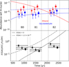 |
Fig. 3 Results of the chemical modeling obtained for the reference model parameters (listed in Table 4) compared with the observations. The curves shows the predicted abundances (relative to H-nuclei) of GA (blue) and ethanol (red) in the upper panel, and the GA/ethanol abundance ratios in the lower panel as a function of time. The symbols represent the values assuming Tex equal to 15 (crosses), 30 (triangles) and 50 (squares) K, as measured at B0, B1 ans B2, respectively. The solid lines correspond to the reference model without GA injection from the dust grains, whereas the dashed lines correspond to the reference model with an injected GA abundance X(CH2OHCHO) = 1.5 × 10⁻⁸. |
6.2 Grid and best-fit model
As explained in the previous section, we varied the chemical abundances injected at the passage of the shock, along with the physical parameters, over the ranges reported in Table 4. In total, we ran about 100 models. We then identified the best-fitting models by minimizing the variance, χ2, defined as:
 (1)
(1)
where theoi and obsi are the [CH2OHCHO]/[C2H5OH] abundance ratios, which are more constraining and reliable than the absolute abundances, and correspond to the predicted values at the estimated ages the regions B0, B1 and B2, and to those measured. The quantity σi represents the measured uncertainties, which includes both the error in the derived abundance ratio, ∆obs, and the age of the position, as well as the range of the model-predicted values within the age error, ∆ theo :
 (2)
(2)
We find that the models with the set of parameters reported in column five of Table 4, best reproduce the observations. With the exception of the gas temperature and the injected water and ethanol abundances, all other parameters are fairly well constrained and are identical to those of the reference model (Column 2 of Table 4), confirming the robustness of our previous modeling studies (e.g. Podio et al. 2014; Codella et al. 2017; Giani et al. 2025; López-Sepulcre et al. 2024).
The gas temperature (Tgas), the injected water (X(H2O)) and ethanol (X(C2H5OH)) abundances are degenerate, having a substantial impact on the dependency of the ethanol abundance with time and, consequently, on the predicted [CH2OHCHO] / [C2 H5 OH] abundance ratio. In particular, predictions of models with a low water abundance (1.0 × 10⁻⁵) agree better with the observations for relatively low gas temperatures, ≤110 K; intermediate water abundance models (5.0 × 10⁻⁵) require gas temperatures between 100 and 120 K; and high water abundance models (1.0 × 10⁻⁴) require larger gas temperatures, between 115 and 130 K (see Fig. 4, and discussion below).
Models of the CO low to high level J observed lines toward B1 have fairly well constrained the temperature, Tgas ~ 60-80 K (e.g. Lefloch et al. 2012), a value refined to ~90 K by subsequent studies (e.g. Codella et al. 2020). Therefore, we favor models with a reduced injected water abundance (2.5 × 10⁻⁵) relative to the reference model and a Tgas ~ 90 K. This new value of the injected the H2O abundance is consistent with that measured by Busquet et al. (2014) with the Herschel Space Observatory9. Furthermore, we verified that this change does not affect the recent results obtained from the study of formamide in B0, B1 and B2 (López-Sepulcre et al. 2024).
The upper panels of Fig. 4 show two sets of model predictions compared with the observations. The first set assumes a temperature of 100 K and four values for the injected H2O abundances (1.0, 2.5, 5.0 and 10 ×10−5) to illustrate their impact on the predictions. The second set assumes an injected H2O abundance of 2.5 × 10⁻⁵ and four temperature values (80, 90, 100 and 130 K) to illustrate its impact on the predicted abundances. The figure shows that the lower the injected H2O abundance, the slower the destruction of ethanol over time. Similarly, increasing the temperature produces the same effect. This behavior arises from the formation of OH (the major destroyer of ethanol), whose abundance is proportional to that of water present in the gas phase, as discussed in Sect. 5.2. In addition, the dominant OH-formation reactions depend on the inverse of the temperature, i.e. the smaller the temperature the larger the OH abundance10.
In conclusion, assuming that (i) GA is entirely produced by gas phase reactions initiated from injected ethanol, and that (ii) the gas temperature and (iii) ice composition are the same in the three regions, we cannot simultaneously reproduce the GA and ethanol observations of B0, B1 and B2. In other words, one or more of the assumptions may be incorrect. In the following, we discuss each of the three assumptions.
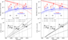 |
Fig. 4 Results obtained assuming that GA forms exclusively in the gas phase via the ethanol tree. Model predictions (curves) are compared with observations (symbols) toward B0, B1 and B2, assuming three excitation temperatures Tex = 15 K (crosses), 30 K (triangles) and 50 K (squares) . In each figure, the upper panels show the abundances of GA (blue) and ethanol (red) as a function of time. The bottom panels show the evolution with time of the GA/ethanol abundance ratio. Left panel: predictions obtained assuming a temperature of 100 K and four values for the injected H2O abundances: 1.0 (dotted), 2.5 (solid), 5.0 (dashed) and 10 (dotted-dashed) ×10−5). Right panel: predictions obtained assuming an injected H2O abundance of 2.5 × 10⁻⁵ and four temperature values: 80 K (dotted), 90 K (dashed), 100 K (solid) and 130 K (dotted-dashed). |
6.3 GA formation on grain surfaces
In the following, we consider the possibility that GA forms on the grain surfaces and is injected into the gas phase at the passage of the shock. Figure 5 compares the observations with the model predictions obtained under the assumption that GA is injected into the gas phase in varying quantities. The gaseous GA is the sum of the injected GA abundance and that produced from ethanol in the gas phase.
To reproduce the range of observed ethanol abundances, we assumed injected ethanol abundances, X(C2H5OH), of 3.0 and 15 ×10−8, and we varied the injected GA abundance from 0 to 8 ×10⁻⁹. The figure shows that only the GA abundance is simultaneously reproduced by the predictions in the three shocked regions when an input of GA from the grain mantles is included, whereas the GA/ethanol abundance ratio is not, for both the low (3.0 × 10⁻⁸) and high (1.5 × 10⁻⁷) ethanol abundances.
In conclusion, assuming that GA is formed on the grain surface does not simultaneously reproduce the observations toward B0, B1 and B2.
6.4 Gas temperature and mantle composition in B0, B1 and B2
To obtain the previous model predictions, we assumed identical temperatures and mantle compositions in the three regions B0, B1 and B2.
However, there is no evidence that the gas in these regions has the same temperature (or density). As shown in Fig. 4, different gas temperatures would lead to different evolutions of the ethanol abundance and, consequently, different GA/ethanol abundance ratios. It is reasonable to expect that the temperature in B0 is higher than in B2, as also discussed by López-Sepulcre et al. (2024). After the passage of the shock, the gas temperature first rises (up to thousands of kelvin) and then decreases (to tens of kelvin) (Gusdorf et al. 2008). The shock evolution timescale and the amplitude of the temperature peak largely depend on the shock velocity, magnetic field, and pre-shock density; the former may span from hundreds to thousands of years before reaching the final temperature. During this period, ethanol may be destroyed much more slowly than assumed in our relatively low-temperature models. There are, however, no measurements of the gas temperature in B0 and B2 (as mentioned in Sect. 2). A major limitation of our modeling is that the physical properties, such as temperature, are kept constant in time. At present, no available tools allow us to vary both the physical conditions of the shock and the gas-phase chemistry simultaneously using the most up-to-date chemical networks.
Regarding the grain mantle composition, the distance between B0 and B2 is about 5000-7000 au, which is, in principle, large enough for the mantle composition to differ in the two regions. However, direct observations of mantle-composition variations in low-mass protostars at these scales do not exist. Evidence based on the deuteration of formaldehyde (H2CO), which changes by more than a factor of two in the protostar NGC1333 IRAS4A over a scale of 4000 au (Chahine et al. 2024), supports the idea of a slightly different grain mantle composition in B0 and B2; however, it is not yet possible to quantify the difference. Another reason for a different mantle composition in B0 and B2 is that the former region has already undergone two shocks, those that have now reached B2 and B1, which may have altered its composition. Finally, the age of B0 may be underestimated, for example if the western part included in the “B0 polygon” actually belongs to B1.
In summary, to determine whether different gas temperatures and/or grain-mantle compositions in B0, B1 and B2 are explain why our model is unable to reproduce the measured GA/ethanol abundance ratio, additional observations (for example, to constrain the temperature and density of B1 and B2) together with more sophisticated time-dependent shock modeling, are required.
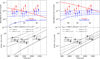 |
Fig. 5 Results obtained assuming that GA forms in the gas phase via the ethanol tree and is injected from the grain mantles into the gas phase at the passage of the shocks. The injected ethanol is 3 × 10⁻⁸ in the left panels and 15 × 10−8 in the right panels. Model predictions (curves) are compared with the observations (symbols) toward B0, B1 and B2, assuming three different excitation temperatures Tex = 15 K (crosses), 30 K (triangles) and 50 K (squares). In each figure, the upper panels show the abundances of GA (blue) and ethanol (red) as a function of time. The bottom panels show the evolution with time of the GA/ethanol abundance ratio. |
7 Conclusions
We mapped the GA and ethanol emission along the L1157 southern outflow with a resolution of ~4″ (equivalent to ~1400 au) using the IRAM NOEMA interferometer. This represents the first spatially resolved map of GA and ethanol in a low-mass protostellar region. Our map covers three different shocked regions; B0, B1 and B2, whose ages, estimated by previous studies, range from ~900 to ~2300 yr. Our conclusions from the observations of these three shocked regions are as follows:
We detected three GA lines and one ethanol line with a S/N > 5 along the L1157 southern outflow, all with similar Eup. While ethanol emission is more or less equally intense across all three shocked regions, GA emission is stronger in B2 than in the other two regions;
Assuming LTE and Tex = 30 K, we derived a GA/ethanol ratio of 0.32 ± 0.07 in B0, 0.23 ± 0.05 in B1, and 0.44 ± 0.09 in B2, showing a slight decrease from B0 and B1 and then an increase between B1 and B2;
The trend between B1 and B2 is consistent with the gasphase formation of GA and can be reproduced by our astrochemical model with an injection of ethanol between 1 and 2 ×10⁻⁷. However, the astrochemical model fails to simultaneously reproduce the observations toward B0, B1 and B2, whether we assume that GA is mostly formed on dust grain surfaces or in the gas phase. This suggests that either our assumptions regarding the same excitation temperature and grain mantle composition in the three shocked regions are incorrect, or that the age of B0 is underestimated, or that varying the physical parameters (e.g., gas temperature and density) over time in the astrochemical model is necessary to reproduce the observations. Future observations targeting additional CH2OHCHO and C2H5OH lines are required to derive the Tex in B0 and in B2;
The GA abundance predicted by our gas-phase astrochemical model is highly sensitive to the gas temperature and the amount of water injected. For Tgas values consistent with those derived in B1 (~100-90K) from previous studies, the injected H2O abundance must be 1-5 ×10⁻⁵. Such relatively low water abundances are required to slow down the gasphase destruction of ethanol and improve the agreement with the observations;
Since ethanol is present in the gas phase with an abundance of about 0.4 and 6 ×10⁻⁸, GA will inevitably be produced by ethanol via the gas-phase reactions of the “ethanol tree”. Therefore, grain-surface formation cannot be a dominant source of gaseous GA in the L1157 outflow shocks;
To date, B1 is by far the most studied shocked region of the L1157 outflow because of its brightness and richness in iCOMs. However, our observations show that, with respect to GA, B2 is the brightest region of the outflow, and may be even richer in iCOMs and is particularly relevant for products that require time to form in the gas phase.
As in previous studies (Podio et al. 2014; Codella et al. 2017; Tinacci et al. 2023; Giani et al. 2023; López-Sepulcre et al. 2024), this work shows the relevance of using protostellar outflows displaying several shocked regions of different ages in order to probe gas-phase chemical evolution with time. Finally, we emphasize the need for self-consistent shock models that simultaneously account for the time evolution of the gas temperature and species abundances, as well as to better constrain the gas temperature and density in B0 and B2.
Acknowledgements
We thank the IRAM-NOEMA staff for their help and support during the observations. We warmly thank Antoine Gusdorf for his precious help and advice on the theoretical aspects of the molecular shocks. We sincerely thank the anonymous referee for careful reading and thoughtful comments. This project has received funding from the European Research Council (ERC) under the European Union’s Horizon 2020 research and innovation program, for the Project “The Dawn of Organic Chemistry” (DOC), grant agreement No. 741002. Linda Podio and Claudio Codella acknowledge the PRIN-MUR 2020 BEYOND-2p (Astrochemistry beyond the second period elements, Prot. 2020AFB3FX), the project ASI-Astrobiologia 2023 MIGLIORA (Modeling Chemical Complexity, F83C23000800005), the INAF-GO 2023 fundings PROTO-SKA (Exploiting ALMA data to study planet forming disks: preparing the advent of SKA, C13C23000770005), the INAF-MiniGrant 2022 “Chemical Origins” (PI: L. Podio), and financial support under the National Recovery and Resilience Plan (NRRP), Mission 4, Component 2, Investment 1.1, Call for tender No. 104 published on 2.2.2022 by the Italian Ministry of University and Research (MUR), funded by the European Union – NextGenerationEU- Project Title 2022JC2Y93 Chemical Origins: linking the fossil composition of the Solar System with the chemistry of protoplanetary disks – CUP J53D23001600006 – Grant Assignment Decree No. 962 adopted on 30.06.2023 by the Italian Ministry of University and Research (MUR). This work made use of ASAI “Astrochemical Surveys At IRAM” (Lefloch, Bachiller, Gonzalez et al. 2017) data.
References
- Anicich, V., Kim, J., & Huntress, W. 1977, Int. J. Mass Spectrom. Ion Phys., 25, 433 [Google Scholar]
- Arce, H. G., Santiago-García, J., Jørgensen, J. K., Tafalla, M., & Bachiller, R. 2008, ApJ, 681, L21 [NASA ADS] [CrossRef] [Google Scholar]
- Ascenzi, D., Cernuto, A., Balucani, N., et al. 2019, A&A, 625, A72 [NASA ADS] [CrossRef] [EDP Sciences] [Google Scholar]
- Bachiller, R., Liechti, S., Walmsley, C. M., & Colomer, F. 1995, A&A, 295, L51 [NASA ADS] [Google Scholar]
- Bachiller, R., & Pérez-Gutiérrez, M. 1997, in Herbig-Haro Flows and the Birth of Stars, 182, eds. B. Reipurth, & C. Bertout, 153 [Google Scholar]
- Balucani, N., Ceccarelli, C., & Taquet, V. 2015, MNRAS, 449, L16 [Google Scholar]
- Balucani, N., Ceccarelli, C., Vazart, F., et al. 2024, MNRAS, 528, 6706 [Google Scholar]
- Beltrán, M. T., Codella, C., Viti, S., Neri, R., & Cesaroni, R. 2009, ApJ, 690, L93 [Google Scholar]
- Benedettini, M., Viti, S., Codella, C., et al. 2007, MNRAS, 381, 1127 [Google Scholar]
- Benedettini, M., Viti, S., Codella, C., et al. 2013, MNRAS, 436, 179 [Google Scholar]
- Bohme, D. K., Mackay, G. I., & Tanner, S. D. 1979, J. Am. Chem. Soc., 101, 3724 [CrossRef] [Google Scholar]
- Boogert, A. C. A., Gerakines, P. A., & Whittet, D. C. B. 2015, ARA&A, 53, 541 [Google Scholar]
- Busquet, G., Lefloch, B., Benedettini, M., et al. 2014, A&A, 561, A120 [NASA ADS] [CrossRef] [EDP Sciences] [Google Scholar]
- Caravan, R. L., Shannon, R. J., Lewis, T., Blitz, M. A., & Heard, D. E. 2015, J. Phys. Chem. A, 119, 7130 [Google Scholar]
- Caselli, P., Hartquist, T. W., & Havnes, O. 1997, A&A, 322, 296 [NASA ADS] [Google Scholar]
- Ceccarelli, C. 2023, Astrochemistry at high resolution [Google Scholar]
- Ceccarelli, C., Hollenbach, D. J., & Tielens, A. G. G. M. 1996, ApJ, 471, 400 [Google Scholar]
- Ceccarelli, C., Caselli, P., Fontani, F., et al. 2017, ApJ, 850, 176 [NASA ADS] [CrossRef] [Google Scholar]
- Ceccarelli, C., Viti, S., Balucani, N., & Taquet, V. 2018, MNRAS, 476, 1371 [CrossRef] [Google Scholar]
- Ceccarelli, C., Codella, C., Balucani, N., et al. 2023, in Astronomical Society of the Pacific Conference Series, 534, Protostars and Planets VII, eds. S. Inutsuka, Y. Aikawa, T. Muto, K. Tomida, & M. Tamura, 379 [Google Scholar]
- Chahine, L., Ceccarelli, C., De Simone, M., et al. 2024, MNRAS, 534, L48 [Google Scholar]
- Clary, D. C. 1985, Mol. Phys., 54, 605 [Google Scholar]
- Codella, C., Benedettini, M., Beltrán, M. T., et al. 2009, A&A, 507, L25 [NASA ADS] [CrossRef] [EDP Sciences] [Google Scholar]
- Codella, C., Ceccarelli, C., Caselli, P., et al. 2017, A&A, 605, L3 [NASA ADS] [CrossRef] [EDP Sciences] [Google Scholar]
- Codella, C., Ceccarelli, C., Bianchi, E., et al. 2020, A&A, 635, A17 [NASA ADS] [CrossRef] [EDP Sciences] [Google Scholar]
- Coutens, A., Persson, M. V., Jørgensen, J. K., Wampfler, S. F., & Lykke, J. M. 2015, A&A, 576, A5 [NASA ADS] [CrossRef] [EDP Sciences] [Google Scholar]
- De Simone, M., Codella, C., Testi, L., et al. 2017, A&A, 599, A121 [NASA ADS] [CrossRef] [EDP Sciences] [Google Scholar]
- Enrique-Romero, J., Rimola, A., Ceccarelli, C., et al. 2022, ApJS, 259, 39 [NASA ADS] [CrossRef] [Google Scholar]
- Ferrero, S., Ceccarelli, C., Ugliengo, P., Sodupe, M., & Rimola, A. 2024, ApJ, 960, 22 [NASA ADS] [CrossRef] [Google Scholar]
- Field, D., May, P. W., Pineau des Forets, G., & Flower, D. R. 1997, MNRAS, 285, 839 [Google Scholar]
- Flower, D. R., Pineau des Forets, G., Field, D., & May, P. W. 1996, MNRAS, 280, 447 [Google Scholar]
- Garrod, R., Park, I. H., Caselli, P., & Herbst, E. 2006, Faraday Discuss., 133, 51 [Google Scholar]
- Garrod, R. T., Widicus Weaver, S. L., & Herbst, E. 2008, ApJ, 682, 283 [Google Scholar]
- Garrod, R. T., Jin, M., Matis, K. A., et al. 2022, ApJS, 259, 1 [NASA ADS] [CrossRef] [Google Scholar]
- Geppert, W. D., Hamberg, M., Thomas, R. D., et al. 2006, Faraday Discuss, 133, 177 [Google Scholar]
- Giani, L., Ceccarelli, C., Mancini, L., et al. 2023, MNRAS, 526, 4535 [NASA ADS] [CrossRef] [Google Scholar]
- Giani, L., Bianchi, E., Fournier, M., et al. 2025, MNRAS, 537, 3861 [Google Scholar]
- Gueth, F., Guilloteau, S., & Bachiller, R. 1996, A&A, 307, 891 [NASA ADS] [Google Scholar]
- Gusdorf, A., Cabrit, S., Flower, D. R., & Pineau Des Forêts, G. 2008, A&A, 482, 809 [NASA ADS] [CrossRef] [EDP Sciences] [Google Scholar]
- Halfen, D. T., Apponi, A. J., Woolf, N., Polt, R., & Ziurys, L. M. 2006, ApJ, 639, 237 [CrossRef] [Google Scholar]
- Hama, T., & Watanabe, N. 2013, Chem. Rev., 113, 8783 [Google Scholar]
- Herbst, E., & van Dishoeck, E. F. 2009, ARA&A, 47, 427 [Google Scholar]
- Hollis, J. M., Lovas, F. J., & Jewell, P. R. 2000, ApJ, 540, L107 [Google Scholar]
- Hollis, J. M., Jewell, P. R., Lovas, F. J., & Remijan, A. 2004, ApJ, 613, L45 [Google Scholar]
- Jaber, A. A., Ceccarelli, C., Kahane, C., & Caux, E. 2014, ApJ, 791, 29 [Google Scholar]
- Jalbout, A. F., Abrell, L., Adamowicz, L., et al. 2007, Astrobiology, 7, 433 [Google Scholar]
- Jiménez-Serra, I., Caselli, P., Martin-Pintado, J., & Hartquist, T. W. 2008, A&A, 482, 549 [NASA ADS] [CrossRef] [EDP Sciences] [Google Scholar]
- Jørgensen, J. K., Favre, C., Bisschop, S. E., et al. 2012, ApJ, 757, L4 [Google Scholar]
- Jørgensen, J. K., van der Wiel, M. H. D., Coutens, A., et al. 2016, A&A, 595, A117 [Google Scholar]
- Lefloch, B., Cabrit, S., Busquet, G., et al. 2012, ApJ, 757, L25 [Google Scholar]
- Lefloch, B., Ceccarelli, C., Codella, C., et al. 2017, MNRAS, 469, L73 [Google Scholar]
- Lefloch, B., Bachiller, R., Ceccarelli, C., et al. 2018, MNRAS, 477, 4792 [Google Scholar]
- López-Sepulcre, A., Codella, C., Ceccarelli, C., Podio, L., & Robuschi, J. 2024, A&A, 692, A120 [NASA ADS] [CrossRef] [EDP Sciences] [Google Scholar]
- Mendoza, E., Lefloch, B., López-Sepulcre, A., et al. 2014, MNRAS, 445, 151 [NASA ADS] [CrossRef] [Google Scholar]
- Mikami, H., Umemoto, T., Yamamoto, S., & Saito, S. 1992, ApJ, 392, L87 [Google Scholar]
- Millar, T. J., Walsh, C., Van de Sande, M., & Markwick, A. J. 2024, A&A, 682, A109 [NASA ADS] [CrossRef] [EDP Sciences] [Google Scholar]
- Müller, H. S. P., Belloche, A., Xu, L.-H., et al. 2016, A&A, 587, A92 [NASA ADS] [CrossRef] [EDP Sciences] [Google Scholar]
- Novotny, O., Buhr, H., Stützel, J., et al. 2010, J. Phys. Chem. A, 114, 4870 [Google Scholar]
- Pearson, J. C., Brauer, C. S., & Drouin, B. J. 2008, J. Mol. Spectrosc., 251, 394 [NASA ADS] [CrossRef] [Google Scholar]
- Perrero, J., Enrique-Romero, J., Martínez-Bachs, B., et al. 2022, ACS Earth Space Chem., 6, 496 [NASA ADS] [CrossRef] [Google Scholar]
- Podio, L., Lefloch, B., Ceccarelli, C., Codella, C., & Bachiller, R. 2014, A&A, 565, A64 [NASA ADS] [CrossRef] [EDP Sciences] [Google Scholar]
- Podio, L., Codella, C., Gueth, F., et al. 2016, A&A, 593, L4 [NASA ADS] [CrossRef] [EDP Sciences] [Google Scholar]
- Rimola, A., Taquet, V., Ugliengo, P., Balucani, N., & Ceccarelli, C. 2014, A&A, 572, A70 [NASA ADS] [CrossRef] [EDP Sciences] [Google Scholar]
- Skouteris, D., Balucani, N., Ceccarelli, C., et al. 2018, ApJ, 854, 135 [NASA ADS] [CrossRef] [Google Scholar]
- Spanel, P., & Smith, D. 1997, Int. J. Mass Spectrom. Ion Processes, 167, 375 [CrossRef] [Google Scholar]
- Tafalla, M., & Bachiller, R. 1995, ApJ, 443, L37 [Google Scholar]
- Taquet, V., Ceccarelli, C., & Kahane, C. 2012, ApJ, 748, L3 [Google Scholar]
- Taquet, V., Charnley, S. B., & Sipilä, O. 2014, ApJ, 791, 1 [NASA ADS] [CrossRef] [Google Scholar]
- Taquet, V., López-Sepulcre, A., Ceccarelli, C., et al. 2015, ApJ, 804, 81 [Google Scholar]
- Tielens, A. G. G. M., & Hagen, W. 1982, A&A, 114, 245 [Google Scholar]
- Tinacci, L., Ferrada-Chamorro, S., Ceccarelli, C., et al. 2023, ApJS, 266, 38 [NASA ADS] [CrossRef] [Google Scholar]
- Tobin, J. J., Chandler, C. J., Wilner, D. J., et al. 2013, ApJ, 779, 93 [Google Scholar]
- Tobin, J. J., Cox, E. G., & Looney, L. W. 2022, ApJ, 928, 61 [NASA ADS] [CrossRef] [Google Scholar]
- Troe, J. 1996, J. Chem. Phys., 105, 6249 [NASA ADS] [CrossRef] [Google Scholar]
- Vasyunin, A. I., & Herbst, E. 2013, ApJ, 769, 34 [Google Scholar]
- Wakelam, V., Gratier, P., Loison, J. C., et al. 2024, A&A, 689, A63 [NASA ADS] [CrossRef] [EDP Sciences] [Google Scholar]
- Weber, A. L. 1998, Origins Life Evol. Biosph., 28, 259 [Google Scholar]
- Widicus Weaver, S. L., Butler, R. A. H., Drouin, B. J., et al. 2005, ApJS, 158, 188 [Google Scholar]
- Woods, P. M., Kelly, G., Viti, S., et al. 2012, ApJ, 750, 19 [NASA ADS] [CrossRef] [Google Scholar]
- Xu, L.-H., Fisher, J., Lees, R. M., et al. 2008, J. Mol. Spectrosc., 251, 305 [NASA ADS] [CrossRef] [Google Scholar]
- Zucker, C., Speagle, J. S., Schlafly, E. F., et al. 2019, ApJ, 879, 125 [NASA ADS] [CrossRef] [Google Scholar]
See Cologne Database for Molecular Spectroscopy (CDMS): https://cdms.astro.uni-koeln.de/classic/predictions/catalog/
Institut de RadioAstronomie Millimétrique: https://iram-institute.org
Cologne Database for Molecular Spectroscopy: https://cdms.astro.uni-koeln.de/classic/predictions/catalog/
We verified that the spectral parameters retrieved from CDMS and used to derive the column densities are consistent with those listed in the JPL spectroscopy database (Jet Propulsion Laboratory: https://spec.jpl.nasa.gov/ftp/pub/catalog/catdir.html).
We verified a posteriori that the lines are indeed optically thin and found τ < 10−3 for the four GA and ethanol lines.
KIDA database: (https://kida.astrochem-tools.org/: Wakelam et al. 2024).
UMIST database: (https://umistdatabase.uk: Millar et al. 2024).
In B1, Busquet et al. (2014) measured a water column density NH2O = (4.0-10) × 1016 cm−2, which implies a water abundance X(H2O) = (1.010) × 10−5, assuming NH ≈ (1-4) × 1021 cm−2.
As discussed in Sect. 5.2, the rate constant for ethanol protonation by H3O+ (reaction 2) may be overestimated by up to a factor of ten. Conversely, decreasing the injected H2O abundance or increasing the gas temperature decreases the GA/ethanol abundance ratio because lowering the injected ethanol abundance would decrease both the gaseous ethanol and GA, leaving their abundance ratio nearly unchanged. For completeness, we ran a model with a reduced rate constant for this reaction and verified that the impact is marginal, as the other two ethanol destruction routes take over and compensate for it.
ASAI data are accessible following this link: https://iram-institute.org/science-portal/proposals/lp/completed/lp007-iram-chemical-survey-of-sun-like-star-forming-regions/
Appendix A Glycolaldehyde emission maps along the entire outflow and spectra in the three shocked regions
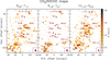 |
Fig. A.1 Maps of the emission of GA along the entire southern outflow of L1157, for all three transitions. The first contours are drawn at 3σ and the following with a step of 1σ (1σ = 0.1 K km s−1 for the 80,8 − 71,7 transition, 0.05 K km s−1 for the S1,s − 70,7 transition and 0.1 K km s−1 for the 101,10 – 90,9 transition). Note that we masked out the noise at the edge of the maps, and that the rms was estimated at the center of the maps; therefore the first contour might be at slightly less than 3σ in B2, which is close to the noisier edge of the maps. |
In this section, we present the emission maps of the three GA lines detected in our data, along the entire southern outflow (Fig. A.1).
On the whole outflow, all three lines are brighter around B2, where they show clear emission. The S0,s – 71,7 and 101,10 – 90,9 lines also display emission around B0c-d and in B1. Although this emission is fainter than in B2, the two lines are clearly detected in these regions (see spectra integrated over the respective polygons in Fig. A.2). However, transition S1,s – 70,7 is not detected in B0 and marginally detected in B1 (see spectra Fig. A.2). Note that the emission of the GA 81,8 – 70,7 transition is also slightly fainter than the other two in the B1 observational data acquired by the large program ASAI (see Sect. B for a comparison with ASAI data). This difference could be due to the low spectral resolution which we are working with (2 MHz) or to the high noise level compared with the line strength.
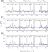 |
Fig. A.2 Spectra of the three GA transitions, obtained by integrating the emission inside the polygons defined for each shocked region. The blue line marks the zero intensity level of each spectrum, and the dotted red line shows the v1sr of L1157-mms, namely 2.6 km s−1 with respect to the Sun. Note that the 81,8 − 70,7 transition is not detected in B0, and is slightly below the 3σ threshold in B1. Please also note that the emission of the GA transition at f = 85 782.24MHz spans over one channel only, whereas the other two GA lines display emission detected in 3 channels. This is likely due to the low intensity of the former and to the low spectral resolution (spectral resolution of 2 MHz, equivalent to ~ 7 km s−1 at 85 782 MHz). |
Appendix B Comparison with ASAI
In order to estimate the fraction of flux filtered out by the interferometer, we compared our results, obtained with the interferometer NOEMA, to those of the large program ASAI (Astrochemical Surveys At IRAM, Lefloch et al. 2017, 2018). Indeed, the shocked region B1 located in the southern molecular outflow of L1157-mms has been observed as part of the ASAI large program with the IRAM 30-meter telescope. Using these observations, Lefloch et al. (2017) detected 14 GA lines and 22 ethanol lines, among which all the lines we detected for these species using NOEMA.
To conduct this comparison, we averaged the flux recovered around B1 in our data over the IRAM 30-meter telescope half-power beam size, and confronted the spectra with those obtained using the ASAI data11 (see Fig. B.1). We then measured the velocity-integrated intensities for each line in both datasets; the results are reported in Table B.1. In the end, we appear to recover the totality of the ASAI flux with our NOEMA observations. We are consistent with ASAI data within 3σ, which comforts us in our detection of GA and ethanol. We also computed the column densities of ethanol and GA in B1, for our and ASAI observations; the results are summarized in Table B.1. The column densities computed for our GA lines detected in B1, are consistent between the two studies within 3σ for an excitation temperature of ~ 30 K (Lefloch et al. 2017). However, the 3σ upper limit on the column density computed using the 81,8 – 70,7 GA transition in the NOEMA data is not consistent with the NCH2OHCHO computed using the two other transitions of this molecule. Note that this line is also relatively faint in ASAI, falling below their best fit line in their rotational diagram. This could be due to non-LTE effects.
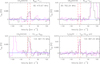 |
Fig. B.1 Spectra obtained with the IRAM 30-meter (in purple) as part of the ASAI large program vs spectra from our observations obtained with the NOEMA radio-interferometer (in black). In order to compare these two datasets, we degraded the spectral resolution of the ASAI data to 2 MHz. The dotted red lines mark the velocity range over which the flux was integrated. The NOEMA spectra were obtained by spatially averaging the flux over the half-power beam size of the IRAM 30-m telescope used for the ASAI observations. The horizontal blue line marks the zero intensity level of each spectrum. |
Properties of the detected lines – Comparison with those of ASAI.
All Tables
Derived properties of the detected line emission in the different shocked regions.
Gas phase chemical reactions involved in the destruction of gaseous ethanol (upper half of the table) and in the formation of gaseous OH, a major ethanol destroyer (lower half of the table).
All Figures
|
Fig. 1 Zoom on the three shocked regions. The left panel shows a zoom on the GA and ethanol emission maps toward B0, B1, and B2, integrated over the velocity range [−10,5] km s−1. The velocity-integrated emission is shown by white and red contours for the GA and ethanol lines, respectively, overlaid on the emission of the CH3OH line 51,5−40,4 in color scale. For the GA and ethanol lines, the first contours are drawn at 3σ and the subsequent contours are plotted in steps of 1σ (1σ = 15 mJy/beam km/s for CH2OHCHO and 12 mJy/beam km/s for C2H5OH in B0 and B1; 18 mJy/beam km/s for CH2OHCHO and 14 mJy/beam km/s for C2H5OH in B2). The ellipses in the corners indicate the synthesized beams for each GA and ethanol line. The white triangles and associated labels mark the different clumps identified by Benedettini et al. (2007). The right panel shows the velocity-integrated intensity map of the CH3OH 51,5−40,4 line, illustrating the morphology of the overall L1157 southern molecular outflow. The methanol map was used to define the polygons (shown by magenta contours) within which the intensities used for the column density computations are integrated (see text). The methanol map is centered at α(J2000) = 20h39m09.635s and δ(J2000) = 68°01′19.80″. The first contour is drawn at 50σ and subsequent contours are plotted in steps of 100σ (1σ = 11 mJy/beam km/s). The black ellipse in the bottom right corner indicates the synthesized beam of the CH3OH line. The white squares centered on B0, B1 and B2 delimit the areas of the zoomed maps shown in the left panels. The white star at the top of the map marks the position of the unresolved L1157 protobinary system (Tobin et al. 2013, 2022). |
| In the text | |
|
Fig. 2 Glycolaldehyde (GA) column density and abundance ratio, computed from the 101,10−90,9 line, which is the brightest, assuming LTE population and optically thin line emission. The bands represent the uncertainty associated with the line intensity (see text). Upper panel: column density of GA in B0 (light pink), B1 (pink) and B2 (dark pink), as a function of the excitation temperature Tex. The column density values partially overlap in B0 and B1. Lower panel: GA/ethanol abundance ratio versus Texc in B0, B1 and B2 (same color coding as above). |
| In the text | |
|
Fig. 3 Results of the chemical modeling obtained for the reference model parameters (listed in Table 4) compared with the observations. The curves shows the predicted abundances (relative to H-nuclei) of GA (blue) and ethanol (red) in the upper panel, and the GA/ethanol abundance ratios in the lower panel as a function of time. The symbols represent the values assuming Tex equal to 15 (crosses), 30 (triangles) and 50 (squares) K, as measured at B0, B1 ans B2, respectively. The solid lines correspond to the reference model without GA injection from the dust grains, whereas the dashed lines correspond to the reference model with an injected GA abundance X(CH2OHCHO) = 1.5 × 10⁻⁸. |
| In the text | |
|
Fig. 4 Results obtained assuming that GA forms exclusively in the gas phase via the ethanol tree. Model predictions (curves) are compared with observations (symbols) toward B0, B1 and B2, assuming three excitation temperatures Tex = 15 K (crosses), 30 K (triangles) and 50 K (squares) . In each figure, the upper panels show the abundances of GA (blue) and ethanol (red) as a function of time. The bottom panels show the evolution with time of the GA/ethanol abundance ratio. Left panel: predictions obtained assuming a temperature of 100 K and four values for the injected H2O abundances: 1.0 (dotted), 2.5 (solid), 5.0 (dashed) and 10 (dotted-dashed) ×10−5). Right panel: predictions obtained assuming an injected H2O abundance of 2.5 × 10⁻⁵ and four temperature values: 80 K (dotted), 90 K (dashed), 100 K (solid) and 130 K (dotted-dashed). |
| In the text | |
|
Fig. 5 Results obtained assuming that GA forms in the gas phase via the ethanol tree and is injected from the grain mantles into the gas phase at the passage of the shocks. The injected ethanol is 3 × 10⁻⁸ in the left panels and 15 × 10−8 in the right panels. Model predictions (curves) are compared with the observations (symbols) toward B0, B1 and B2, assuming three different excitation temperatures Tex = 15 K (crosses), 30 K (triangles) and 50 K (squares). In each figure, the upper panels show the abundances of GA (blue) and ethanol (red) as a function of time. The bottom panels show the evolution with time of the GA/ethanol abundance ratio. |
| In the text | |
|
Fig. A.1 Maps of the emission of GA along the entire southern outflow of L1157, for all three transitions. The first contours are drawn at 3σ and the following with a step of 1σ (1σ = 0.1 K km s−1 for the 80,8 − 71,7 transition, 0.05 K km s−1 for the S1,s − 70,7 transition and 0.1 K km s−1 for the 101,10 – 90,9 transition). Note that we masked out the noise at the edge of the maps, and that the rms was estimated at the center of the maps; therefore the first contour might be at slightly less than 3σ in B2, which is close to the noisier edge of the maps. |
| In the text | |
|
Fig. A.2 Spectra of the three GA transitions, obtained by integrating the emission inside the polygons defined for each shocked region. The blue line marks the zero intensity level of each spectrum, and the dotted red line shows the v1sr of L1157-mms, namely 2.6 km s−1 with respect to the Sun. Note that the 81,8 − 70,7 transition is not detected in B0, and is slightly below the 3σ threshold in B1. Please also note that the emission of the GA transition at f = 85 782.24MHz spans over one channel only, whereas the other two GA lines display emission detected in 3 channels. This is likely due to the low intensity of the former and to the low spectral resolution (spectral resolution of 2 MHz, equivalent to ~ 7 km s−1 at 85 782 MHz). |
| In the text | |
|
Fig. B.1 Spectra obtained with the IRAM 30-meter (in purple) as part of the ASAI large program vs spectra from our observations obtained with the NOEMA radio-interferometer (in black). In order to compare these two datasets, we degraded the spectral resolution of the ASAI data to 2 MHz. The dotted red lines mark the velocity range over which the flux was integrated. The NOEMA spectra were obtained by spatially averaging the flux over the half-power beam size of the IRAM 30-m telescope used for the ASAI observations. The horizontal blue line marks the zero intensity level of each spectrum. |
| In the text | |
Current usage metrics show cumulative count of Article Views (full-text article views including HTML views, PDF and ePub downloads, according to the available data) and Abstracts Views on Vision4Press platform.
Data correspond to usage on the plateform after 2015. The current usage metrics is available 48-96 hours after online publication and is updated daily on week days.
Initial download of the metrics may take a while.