| Issue |
A&A
Volume 706, February 2026
|
|
|---|---|---|
| Article Number | A186 | |
| Number of page(s) | 27 | |
| Section | Extragalactic astronomy | |
| DOI | https://doi.org/10.1051/0004-6361/202556206 | |
| Published online | 10 February 2026 | |
Duration and properties of the embedded phase of star formation in 37 nearby galaxies from PHANGS-JWST
1
Zentrum für Astronomie der Universität Heidelberg, Institut für Theoretische Astrophysik Albert-Ueberle-Str. 2 69120 Heidelberg, Germany
2
Cosmic Origins Of Life (COOL) Research DAO, https://coolresearch.io, Germany
3
Kavli Institute for Particle Astrophysics & Cosmology, Stanford University CA 94305, USA
4
INAF – Osservatorio Astrofisico di Arcetri Largo E. Fermi 5 I-50125 Florence, Italy
5
European Southern Observatory Karl-Schwarzschild Straße 2 D-85748 Garching bei München, Germany
6
Department of Physics, University of Arkansas, 226 Physics Building 825 West Dickson Street Fayetteville AR 72701, USA
7
Université Côte d’Azur, Observatoire de la Côte d’Azur, CNRS, Laboratoire Lagrange 06000 Nice, France
8
Department of Astronomy, The Ohio State University 140 West 18th Avenue Columbus OH 43210, USA
9
Department of Physics and Astronomy, University of Wyoming Laramie WY 82071, USA
10
Department of Astronomy, University of Cape Town Rondebosch 7701 Cape Town, South Africa
11
Astronomisches Rechen-Institut, Zentrum für Astronomie der Universität Heidelberg Mönchhofstraße 12-14 D-69120 Heidelberg, Germany
12
Research School of Astronomy and Astrophysics, Australian National University Canberra ACT 2611, Australia
13
ARC Centre of Excellence for All Sky Astrophysics in 3 Dimensions (ASTRO 3D), Australia
14
Dept. of Physics, University of Alberta, 4-183 CCIS Edmonton Alberta T6G 2E1, Canada
15
Gemini Observatory/NSF NOIRLab 950 N Cherry Avenue Tucson AZ 85719, USA
16
Department of Astronomy & Astrophysics, University of California, San Diego 9500 Gilman Dr. La Jolla CA 92093, USA
17
Center for Cosmology and Astroparticle Physics 191 West Woodruff Avenue Columbus OH 43210, USA
18
Instituto de Astronomía, Universidad Nacional Autónoma de México Ap. 70-264 04510 CDMX, Mexico
19
Max-Planck-Institut für Astronomie Königstuhl 17 D-69117 Heidelberg, Germany
20
Department of Physics, Tamkang University, No.151, Yingzhuan Road Tamsui District New Taipei City 251301, Taiwan
21
Department of Physics and Astronomy, The Johns Hopkins University Baltimore MD 21218, USA
22
Department of Astrophysical Sciences, Princeton University 4 Ivy Lane Princeton NJ 08544, USA
23
Whitman College 345 Boyer Avenue Walla Walla WA 99362, USA
24
Space Telescope Science Institute 3700 San Martin Drive Baltimore MD 21218, USA
25
Sub-department of Astrophysics, Department of Physics, University of Oxford Keble Road Oxford OX1 3RH, UK
★ Corresponding author: This email address is being protected from spambots. You need JavaScript enabled to view it.
Received:
1
July
2025
Accepted:
3
December
2025
Abstract
Light reprocessed by dust grains emitting in the infrared enables the study of the physics at play in dusty embedded regions, where ultraviolet and optical wavelengths are attenuated. Infrared telescopes such as JWST have made it possible to study the earliest feedback phases, when stars are shielded by cocoons of gas and dust. Comprehending this phase is crucial for unravelling the effects of feedback from young stars that leads to their emergence and the dispersal of their host molecular clouds. Here we show that the transition from the embedded to the exposed phase of star formation is short (< 4 Myr) and sometimes almost absent (< 1 Myr) across a sample of 37 nearby star-forming galaxies covering a wide range of morphologies, from massive barred spirals to irregular dwarfs. The short duration of the dust-clearing timescales suggests a predominant role of pre-supernova feedback mechanisms in revealing newborn stars, confirming previous results on smaller samples and allowing, for the first time, a statistical analysis of their dependencies. We find that the timescales associated with mid-infrared emission at 21 μm, tracing a dust-embedded feedback phase, are controlled by a complex interplay between giant molecular cloud properties (masses and velocity dispersions) and galaxy morphology. We report relatively longer durations of the embedded phase of star formation in barred spiral galaxies, while this phase is significantly reduced in low-mass irregular dwarf galaxies. We discuss tentative trends with gas-phase metallicity, which may favor faster cloud dispersal at low metallicities.
Key words: methods: statistical / ISM: clouds / dust / extinction / galaxies: star formation / infrared: ISM
Kavli Postdoctoral Fellow.
ARC DECRA Fellow.
NASA Hubble Fellow.
© The Authors 2026
 Open Access article, published by EDP Sciences, under the terms of the Creative Commons Attribution License (https://creativecommons.org/licenses/by/4.0), which permits unrestricted use, distribution, and reproduction in any medium, provided the original work is properly cited.
This article is published in open access under the Subscribe to Open model. This email address is being protected from spambots. You need JavaScript enabled to view it. to support open access publication.
1. Introduction
Feedback from massive stars on the surrounding interstellar medium (ISM) is a key element regulating the flow of matter and energy within galaxies and, in turn, their global evolution. Importantly, the various feedback mechanisms at play at different stages of stellar evolution may prevent the accretion of new gas onto giant molecular clouds (GMCs) and may be responsible for the low star-formation efficiencies observed in both Galactic and extra-galactic GMCs (e.g., Evans et al. 2009; Schruba et al. 2019; Kruijssen et al. 2019b). Understanding which feedback mechanisms (e.g., winds, shocks, radiative feedback, supernovae) dominate in the different evolutionary stages of GMCs represents an important step in deepening our understanding of the cycle of matter in galaxies and how star formation influences galactic evolution (e.g., Chevance et al. 2023).
Until recently, the studies able to reach the spatial resolutions necessary to distinguish individual GMCs (∼50–100 pc) were restricted to a handful of nearby galaxies (e.g., Wong et al. 2011; Nieten et al. 2006; Engargiola et al. 2003; Gratier et al. 2010; Leroy et al. 2006; Schinnerer et al. 2013; Pety et al. 2013; Bigiel et al. 2008; Leroy et al. 2017; Kruijssen et al. 2019b; Querejeta et al. 2023). However, recent efforts focused on building representative statistical samples of star-forming regions in nearby star-forming galaxies have enabled the assembly of unprecedentedly large catalogs of molecular clouds (e.g., Colombo et al. 2014; Rosolowsky et al. 2021, Hughes et al. in prep.), H II region catalogs (e.g., Espinosa-Ponce et al. 2020; Congiu et al. 2023; Groves et al. 2023; Lugo-Aranda et al. 2024), and stellar clusters (e.g., Adamo et al. 2017; Cook et al. 2019; Maschmann et al. 2024), which can be crossmatched (e.g., Zakardjian et al. 2023). In particular, the Physics at High Angular resolution in Nearby GalaxieS (PHANGS)1 survey contains the ideal sample of galaxies to perform a detailed comparison of star-forming regions probed through the emission of multiple ISM tracers observed at high-angular resolution, with a continuous wavelength coverage from radio to ultraviolet (UV) with telescopes such as ALMA (Leroy et al. 2021), MUSE (Emsellem et al. 2022), HST (Lee et al. 2022), and JWST (Lee et al. 2023; Chown et al. 2025). Current PHANGS catalogs include several tens of thousands of GMCs extracted out of 88 galaxies characterized at ∼50–100 pc scales (Rosolowsky et al. 2021), a similarly large number of individual H II regions extracted from a subsample of 19 galaxies at a median spatial scale of ∼70 pc (Santoro et al. 2022), and ∼100 000 stellar clusters and compact associations identified in a subsample of 38 galaxies (Maschmann et al. 2024).
While several techniques can be used to age-date young stellar associations (e.g., Miret-Roig et al. 2024) and the expanding shells of gas around them (e.g., Bonne et al. 2023; Watkins et al. 2023), deriving direct measurements of the evolutionary timescales is challenging at galactic scales. Nevertheless, the access to high spatial resolution data has enabled the development of different methods to indirectly reconstruct the temporal evolution of star-forming regions (see, e.g., the review in Schinnerer & Leroy 2024). One approach consists of defining subregions within galaxies in an agnostic way by calculating the luminosity-weighted properties of the ISM within geometrical patterns of a fixed size, including the timescales associated with the dynamical state of molecular clouds (such as the gravitational free fall time and the turbulent crossing time; Sun et al. 2022). Other avenues that have been followed include either focusing on the kinematics of large-scale gas flow (Meidt et al. 2015) or leveraging the spatial distribution of different tracers of the stars and gas, assumed to be emitted in a continuous time sequence (see, e.g., the review from Chevance et al. 2023). The above perspective enables a quantitative interpretation of the deviations from the Schmidt-Kennicutt relation (e.g., Kennicutt 1998; de los Reyes & Kennicutt 2019; Kennicutt & De Los Reyes 2021), which are revealed by the observation of clear spatial offsets between star and gas tracers when focusing on resolutions smaller than the typical GMC separation (≤200 pc) or on individual lines of sight (see e.g., Bigiel et al. 2008; Blanc et al. 2009; Onodera et al. 2010; Gratier et al. 2012; Schruba et al. 2010; Leroy et al. 2013; Kruijssen & Longmore 2014; Kreckel et al. 2018; Kruijssen et al. 2019b; Schinnerer et al. 2019; Pan et al. 2022). A statistical analysis of these spatial correlations and decorrelations has been formalized in Kruijssen & Longmore (2014) and Kruijssen et al. (2018), and we describe this analysis in Section 3.3.
This statistical method has been extensively applied to both observations of local galaxies (e.g., Kruijssen et al. 2019b; Chevance et al. 2020a,b, 2022; Zabel et al. 2020; Kim et al. 2021, 2022, 2023; Ward et al. 2020, 2022; Lu et al. 2022; Kruijssen et al. 2024; Romanelli et al. 2025; Kim et al. 2025) and to simulations (e.g., Haydon et al. 2020; Fujimoto et al. 2019; Semenov et al. 2021; Keller et al. 2022). These results depict a baryon cycle in which typical molecular clouds are short-lived (5–30 Myr) and form stars with low integrated star-formation efficiencies (1–8%; see, e.g., Chevance et al. 2020a; Kim et al. 2022). What is more, the feedback timescales, measured using Hα as a star-formation tracer, are short and typically between 1 − 6 Myr, hinting at a predominant role of the pre-supernova feedback mechanisms (e.g., photoionization, stellar winds, radiation pressure) since molecular clouds are dispersed on timescales shorter than (or comparable to) the first supernova explosion (e.g., Chevance et al. 2020a, 2022; Kim et al. 2022). Disentangling the impact of winds from young stars and radiative stellar feedback requires probing the earliest stages of stellar feedback, including the dust-embedded phase of star formation. In particular, star-formation rate (SFR) tracers emitting in the mid-infrared (IR) domain are critical to solving long-standing questions regarding the exact nature of the feedback mechanisms responsible for this fast GMC dispersion while also accounting for extinction effects related to the presence of dust grains in star-forming regions.
The advent of JWST has granted access to high-resolution mid-IR tracers that offer invaluable insights into the earliest stages of star-formation. Such analyses are challenging due to the complex origin of the mid-IR emission, which correlates both with classical molecular gas tracers such as CO (Leroy et al. 2023a,b; Chown et al. 2025), indicating that the mid-IR can be considered as a tracer of the gas column density, and with the attenuation-corrected Hα emission (Leroy et al. 2023b), because it is sensitive to local heating of the dust grains in star-forming regions. As such, the mid-IR emission arises from the combined emission of diffuse gas reservoirs and compact star-forming regions, which contribute in roughly similar proportions (Leroy et al. 2023b; Pathak et al. 2024). Among the different photometric bands observable in the mid-IR, the continuum-dominated bands around ∼20 μm (e.g., WISE/22 μm, MIPS/24 μm, MIRI/21 μm) have been extensively used to correct the SFR estimates for dust-attenuation in H II regions (e.g., Calzetti et al. 2007; Leroy et al. 2012; Kennicutt et al. 2007; Whitcomb et al. 2023; Belfiore et al. 2023b) and to locate the sites of embedded star formation (e.g., Gratier et al. 2012; Corbelli et al. 2017; Kim et al. 2021, 2023). Focusing on the latter, Kim et al. (2021) used the compact Spitzer/24 μm emission in five nearby galaxies to measure the duration of the heavily obscured star-formation phase (tobscured), finding values ranging from 1.4 to 3.8 Myr. The first analysis carried out with the PHANGS-JWST sample (Lee et al. 2023; Chown et al. 2025) suggested that the deeply embedded phase of star formation may indeed be short-lived, but it was restricted to a single measurement obtained for NGC 628 (tobscured = 2.3 Myr; Kim et al. 2023). In this paper, we extend the analysis of the embedded phase of star formation to the largest sample to date, consisting of 37 galaxies drawn from the PHANGS surveys, for which sufficiently high spatial resolution can be probed in CO, Hα, and 21 μm. For the first time, this allows for analysis of the statistical properties of the timescales associated with the dust-emitted 21 μm band and their dependence on various physical parameters that may control the earliest phases of feedback.
These longer mid-IR wavelengths, which are associated with dust-continuum emission that is powered by stochastic heating of very small grains, are preferred to other mid-IR bands that reflect the processing of carbonaceous dust through the emission of aromatic and aliphatic features that are attributed to sub-nanometer polycyclic aromatic hydrocarbon-like molecules (PAHs; Leger & Puget 1984) or hydrogenated amorphous carbons (Jones et al. 1990). We refer to Kim et al. (2025) for a detailed analysis of the timescales associated with PAH-tracing bands. The authors follow a similar framework as the one we used in this study. We also note that the emission associated with PAH can be used to pinpoint the location of embedded young stellar clusters at the highest angular resolution achievable with JWST, providing complementary and independent timescale measurements, which we compare to our approach.
The paper is organized as follows: In Sect. 2 we describe the multiwavelength data used in this analysis. Section 3 presents the methods used to measure timescales. Our main results are presented in Section 4 and discussed in Section 5. In Sect. 6 we summarize our findings and future prospects.
2. Data
2.1. Sample selection
Our sample consists of 37 galaxies, drawn from the PHANGS surveys, which gathers multiwavelength observations of nearby star forming disk galaxies obtained at high spatial resolution, probing physical scales of 30–250 pc. These surveys have targeted relatively massive galaxies, with our final sample covering stellar masses between 109.4 − 1011 M⊙, specific star-formation rates (sSFR) between 10−11 − 10−9.6 yr−1, having moderate inclination (i ≤ 70 deg) and located within 23.5 Mpc (Leroy et al. 2021). They cover a wide range of morphologies, ranging from irregular to flocculent, barred, and grand-design spirals, corresponding to Hubble morphological T-type from 1.2 to 7.4 in the HyperLEDA database (Paturel et al. 2003a,b; Makarov et al. 2014).
In the current study we aim at characterizing the evolutionary timeline of molecular clouds, including their embedded star-forming phase during which young stars are not yet visible in the UV/optical domain. Our analysis focusing on timescale measurement based on the spatial decorrelation between SFR and gas tracers requires the combination of tracers associated with the emission from different ISM phases, as illustrated in Figure 1: the ALMA/CO(2–1) (shown in red) from the PHANGS-ALMA survey (Leroy et al. 2021), the Hα emission (shown in blue) from ground-based observations (Razza et al. subm.), and the dust-emitted 21 μm band (shown in green) from the PHANGS-JWST Cycle 1 Treasury (Lee et al. 2023) and PHANGS-JWST Cycle 2 Treasury (Chown et al. 2025). More information about the different surveys and the data reduction is provided in Section 2.2.
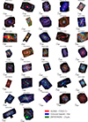 |
Fig. 1. Composite image of the 37 galaxies drawn from the PHANGS surveys, ordered following their Hubble morphological T-type from the LEDA database, from massive spirals to low-mass irregular galaxies. All the maps have been convolved to the resolution of the ALMA/CO(2–1) maps, corresponding to the minimal aperture size reported in Table B.1. The white masks show regions that are excluded from our analysis (Hα and CO bright peaks identified in K22 as well as artifacts and diffraction spikes in any of the three tracers). The green circles show the brightest peaks in 21 μm, which are masked in our analysis, as described in Section 3.1. The number of masked peaks and corresponding surface brightness thresholds are reported in the Table B.1. |
Our sample is drawn from the Kim et al. (2022) sample, hereafter K22, composed of 54 galaxies, observed in CO and Hα, 52 of which have been observed at 21 μm as part of the PHANGS-JWST surveys. We then excluded 15 galaxies for which the physical resolution is insufficient to robustly characterize the decorrelation between CO and 21 μm peaks of emission, yielding a final sample of 37 galaxies, which are listed in Table B.1. Our precise selection criteria are further detailed in Section 4.1.1. We further discuss the reasons why a decorrelation is not observed in a few galaxies from our initial sample and how the resolution of the gas tracers limits the applicability of the method used in this paper in Section 5.3.
2.2. Multiwavelength tracers of the GMC evolution
The observations used in the current study consist in the full-set multiwavelength observations, gathered as part of different PHANGS surveys obtained with a variety of telescope such as ALMA, ground-based facilities targeting Hα, and JWST. We also use ISM properties derived based on the MUSE observation, available for 20/37 galaxies in our sample, as part of the PHANGS-MUSE survey (Emsellem et al. 2022) and its recent extension to lower-mass galaxies (PHANGS-dwarf survey, Egorov et al. in prep.).
2.2.1. Tracers of the molecular gas and of the exposed phase of star formation
Our work builds upon the analysis from K22 and uses the exact same datasets to characterize the timescales associated with the evolution of GMCs based on their CO and Hα observations. As a proxy to trace the cold molecular gas, we use the CO(2–1) maps which were observed as part of the PHANGS-ALMA survey (Leroy et al. 2021). Data reduction is described in detail in Leroy et al. (2021). In this study, we used the maps resulting from a combination of 12-m, 7-m, and total power antennas of ALMA. The maps have a resolution of ∼1″, resulting in a physical scale of ∼25–180 pc for the galaxies considered here. We use the first public release version of moment-0 maps generated with an inclusive signal masking scheme to ensure a high detection completeness (the ‘broad’ masking scheme; see Leroy et al. 2021), at native resolution.
Throughout the paper, the exposed phase of star formation refers to the timescale associated with Hα visibility, while the exposed feedback phase traces the overlap time between the CO and Hα tracers. We use the continuum-subtracted narrowband Hα imaging from PHANGS–Hα (Razza et al. subm.). We note that maps of Hα obtained with MUSE at higher sensitivity, and probing more of the diffuse emission, are available for a subsample of 20/37 galaxies, which are covered with MUSE (Emsellem et al. 2022, Egorov et al. in prep). However, such data are not available for the entire sample of galaxies considered here and updating to Hα maps observed at higher sensitivity is not crucial in our study, since our analysis focuses only on the compact part of the emission and filters out the diffuse contribution, as further described in Section 3.2. We favor homogeneity within our sample and consistency with the previous study from K22 and decide to keep the same set of Hα observations.
2.2.2. 21 μm as tracer of the embedded star formation
To extend the previous analysis of K22, we include an additional proxy of the SFR available in the mid-IR. Specifically, we use the 21 μm associated with dust-continuum emission as a proxy for dust-embedded star formation and refer to the embedded feedback phase as the time when both 21 μm and CO are simultaneously visible, regardless of Hα being detected. We further refer to the “obscured” phase of star formation when only 21 μm is visible without Hα. The MIRI/21 μm observations are drawn from the JWST-PHANGS surveys (Cycle 1; GO #2107, Lee et al. 2023 and Cycle 2, GO #3707, PI: Leroy, Chown et al. 2025), that observed a subsample of the PHANGS-ALMA survey in the near-IR with MIRI and NIRCam. We focus on the MIRI/21 μm maps obtained at a spatial resolution of 0.67″(Lee et al. 2023). A detailed overview of the data reduction can be found in Williams et al. (2024), and the entire PHANGS-JWST sample is presented in Chown et al. (2025).
2.3. Updated maps of ISM properties
A few key physical quantities were updated to more recent measurements compared to K22. We briefly describe these updates in this section.
2.3.1. Total SFR
In order to derive the total SFR within the field of view considered in our analysis and compare it to the previous analysis from K22, we use the SFR maps from the z0mgs atlas (Leroy et al. 2019), that combine maps from the Galaxy Evolution Explorer (GALEX) far ultraviolet band (155 nm) and the Wide-field Infrared Survey Explorer (WISE) W4 band (22 μm), convolved to 15″ angular resolution. For the galaxies which have no GALEX observations, we use instead the SFR maps (Kreckel and Blanc, private communication) derived from PHANGS-Hα ground-based imaging (Razza et al. subm), corrected for extinction using WISE W4 band. The derived SFRs include global corrections for Hα transmission losses and [N II] contamination. We note that these maps were previously used in K22 and that using the same prescription to compute the total SFR and total SFR surface density enable a meaningful comparison of the differences between both study (as described in Section 3.1). Nevertheless, we also consider updated prescriptions for the SFR surface density measured at kiloparsec-scales ( ) based on Belfiore et al. (2023a). We refer to Sun et al. (2023) and Belfiore et al. (2023a) for a comparison of the latter calibration method with other SFR proxies. We note that a constant scaling difference in the total SFR and ΣSFR does not affect the timescale measurements presented in Section 4.
2.3.2. Metallicity
For most of the galaxies in our sample (20/37), we have access to gas-phase metallicity estimates based on MUSE observations from the PHANGS-MUSE survey (Emsellem et al. 2022), covering 15 galaxies from our sample (NGC 1512, NGC 1433, NGC 3351, NGC 3627, NGC 7496, NGC 1365, NGC 4321, NGC 1566, NGC 4303, NGC 1300, NGC 2835, NGC 1087, NGC 0628, NGC 1385, NGC 5068) and from Egorov et al. (in prep), covering five additional galaxies (IC 1954, NGC 3596, NGC 4496A, NGC 4731, and NGC 4781). For the 15 galaxies from PHANGS-MUSE, we estimate the metallicity based on the H II region catalogs from Groves et al. (2023), which report metallicity estimates based on the strong line “S” calibration from Pilyugin & Grebel (2016). The latter estimates are available in the megatables v4p02, following the data aggregation and table creation schemes described in Sun et al. (2022) and Sun et al. (2023). We then calculate the average metallicity as a  -weighted average, excluding the hexagons corresponding to the galactic centers. The resulting metallicity is in excellent agreement with the values obtained by masking and averaging the metallicity from Williams et al. (2022) (smoothed using a Gaussian Process Regression) and the metallicities at the median galactocentric radius from Santoro et al. (2022), both derived using the same MUSE data (see Appendix C, Figure C.1). We use a similar method to derive the metallicities for the five galaxies from Egorov et al. (in prep.).
For the remaining galaxies (17/37) for which no MUSE observations are available, we derived a first-order metallicity estimate based on the stellar-mass metallicity relation from Sánchez et al. (2019) at the effective radius Reff, adopting a metallicity gradient of −0.1 dex/Reff (Sánchez et al. 2014). A comparison of the latter metallicity estimate, based on the stellar mass-metallicity relations, with the direct metallicity measurements from MUSE is provided in Figure C.1. Considering the large uncertainties on these estimates, the latter metallicities are only used as luminosity-weighted galactic averages in order to derive the CO-to-H2 conversion factors (from Section 2.3.3) and the reference timescales (from Section 3.4), but are discarded in the analysis of tentative trends observed between timescales and metallicity from Sections 4 and 5.
2.3.3. CO-to-H2 conversion factor
For the PHANGS-MUSE subsample, we used metallicity-dependent αCO maps, based on MUSE metallicity maps from Williams et al. (2022) and the conversion factor prescription from Bolatto et al. (2013). These maps are obtained by reprojecting the metallicity maps to match the coordinate grid corresponding to the PHANGS-ALMA CO maps. A local conversion factor was then calculated based on Equation 31 from Bolatto et al. (2013), assuming ΣGMC = 100 M⊙ pc−2. The total surface density term includes molecular gas (CO), atomic gas (H I), and stellar mass (IRAC 3.6 μm or WISE 3.4 μm). The conversion factor is then iteratively solved for as described in Sun et al. (2022) (also J. Sun et al., in prep.).
For the remaining galaxies, we followed the same approach as previously used in K22 and estimated a galactic-averaged CO-to-H2 conversion factor based on the prescription from Sun et al. (2020b) and previously used in K22:
 (1)
(1)
where R21 is the CO(2–1)-to-CO(1–0) line ratio (0.65; Leroy et al. 2013; den Brok et al. 2021; Leroy et al. 2022) and Z′ is the CO luminosity-weighted metallicity in units of the solar value3. This relation is applied to the global metallicity estimates derived using the mass-metallicity relation and assuming a negative metallicity gradient of −0.1 dex/kpc. Despite not accounting precisely for the local metallicity variations within each galaxy and assuming a fixed R21 ratio (which incorporates systematic uncertainties, see e.g., Schinnerer & Leroy 2024), this formula provides a reasonable estimate of the global CO-to-H2 conversion factor, accounting for the metallicity dependencies with a slope corresponding to Accurso et al. (2017).
Comparing the H2 mass estimates derived for galaxies where metallicity-dependent CO-to-H2 maps are available to the predictions obtained with a single galactic-average CO-to-H2 conversion factor, we find that taking the average αCO value from Equation 1 may overestimate the local CO-to-H2 conversion factor by up to a factor of three, resulting in an overestimation of the total H2 masses (up to a factor of three) and H2 surface densities (up to a factor of two, as shown in the Appendix C, Figure C.2). We note that, while the CO-to-H2 prescription is important to derive the total H2 mass and H2 surface density, the adopted value does not affect our timescale measurements because the conversion factors cancel each other when we take the ratio of depletion timescales on local and large scales.
3. Methodology
3.1. Data homogenization
Our analysis takes advantage of the rich data available for nearby galaxies by combining maps obtained with different instruments and beam sizes. In order to allow for a meaningful comparison of the peaks of emission identified in different maps, it is then necessary to homogenize the datasets used in the analysis. To do so, we follow the same procedure as detailed in K22, by convolving all the maps to the coarsest resolution, following Aniano et al. (2011), and applying a regridding to ensure that both maps share the same pixel size. The JWST point spread function at 21 μm is computed following the procedure described in Williams et al. (2024) and publicly available as a python package4, which uses the WebbPSF simulation tool (Perrin et al. 2014) version 1.2.1, taking the detector effects into account. The kernels obtained at 21 μm are used to convolve to the ALMA point-spread-function, which is assumed to be Gaussian. The two maps are then reprojected to a common pixel grid using the reproject_interp function from astropy.
The analysis is restricted to regions where all three CO, Hα, and 21 μm were observed. We note that, effectively, smaller field of views are considered compared to K22. In addition, the statistical method used in this study aims at providing averaged parameters over typical star-forming regions; hence, bright peaks of emission in any of the three tracers are systematically masked. To do so, we follow the same approach as presented in K22, by ordering the peaks from the brightest to dimmest and looking for a sharp break in the intensity distribution of peaks. This typically results in a maximum of three masked peaks in Hα or CO in any galaxy, which are shown as white circles in Figure 1. We updated these masks in order to also exclude bright peaks in the 21 μm maps, following the same method, which results on average in masking two additional peaks in 21 μm (shown as green circles in Figure 1). The exact number of masked peaks and the corresponding thresholds in surface brightness are reported in Table B.1. Although such peaks account for only a small fraction of the total number of peaks (typically ≤1%, and ≤3% for all galaxies), they contribute disproportionately to the total compact 21 μm flux. Since the derived timescales are flux-weighted, including them biases the measurements, which become less representative of the averaged cloud population. We further detail the biases introduced by the inclusion of overly bright 21 μm peaks in Appendix D.
Following K22, we also mask the galactic centers, which are affected by blending. We note that masking the central regions of galaxies exclude a significant fraction of the total flux of the galaxies, making our analysis only representative of the star-formation timeline in the outer parts of galaxies. The final masks, that include masks of the galactic centers affected by blending, as well as masks of bright peaks and regions affected by instrumental effects such as diffraction spikes, are shown in Figure 1. These slight modifications of the masked regions, as well as the new prescriptions adopted for metallicity and the CO-to-H2 conversion factors (see Section 2.3) involve moderate variations of the predicted parameters compared to the previous analysis from K22, which are further discussed in the Appendix C.
3.2. Filtering diffuse emission
In order to characterize the evolution timeline of molecular clouds, we want to focus on the emission arising from molecular clouds and H II regions only. As a result, we consider only the spatially compact emission concentrated around the peaks, identified using the CLUMPFIND (Williams et al. 1994) algorithm (∼60 − 750 peaks identified in each tracer per galaxy), while removing possible contribution from more diffuse neutral and ionized gas components. The peak identification is performed by CLUMPFIND by calculating flux contour levels in each map, assuming a given range and interval for each tracer in logarithmic scales. The logarithmic ranges and logarithmic intervals below flux maximum covered by flux contour levels for the identification of CO and 21 μm peaks are reported in Table B.1.
To contrast the Hα and 21 μm emission with the CO emitting molecular gas, we are only interested in the fraction of this emission that is directly associated with the ongoing star-formation cycle, i.e., the compact emission. Nevertheless, diffuse emission can contaminate CO, Hα, and 21 μm. Focusing on the recent MUSE/Hα observations available for 19 galaxies, Belfiore et al. (2022) report that diffuse ionized gas contributes to 19 − 55% of the total Hα emission. The diffuse emission in 21 μm is even larger, with the emission powered by diffuse interstellar radiation field contributing up to ∼50–60% to the total emission (e.g., Belfiore et al. 2023b; Pathak et al. 2024).
Several strategies have been proposed to correct for the diffuse emission. In this work, we follow the methodology developed in Hygate et al. (2019), by filtering the diffuse component in Fourier space using a Gaussian high-pass filter, characterized by a critical distance in frequency space. Following the recommendations from Hygate et al. (2019), we ensure that the relative flux losses in compact regions due to the Fourier filtering are less than 10% in all three tracers. In the current study, we use a softening parameter, nλ, (see values reported in Appendix B, Table B.1), that filters out the emission on scales nλ times larger than the typical distance between peaks. Effectively, we filter out the emission on scales larger than ∼1 − 3 kpc. This filtering is carried out iteratively while updating λ, until it converges toward a fixed value. This procedure allows us to separate the compact component from the diffuse component in the different emission maps. We discuss the variations in the fractions of diffuse 21 μm emission (f ) in Section 4.2.4. An illustration of the compact emission maps, obtained after this filtering, is presented for four galaxies in Figure B.1.
3.3. Measuring evolutionary timescales
In the following, we briefly recall the main steps implemented within the HEISENBERG code (Kruijssen et al. 2018), which is publicly available on GitHub5. In the current study, we combined updated results from the analysis of K22 using Hα as SFR tracer to new runs and leveraging 21 μm as an SFR tracer, which we further describe in this section. The relative timescales were derived based on the spatial distribution of the peaks of emission, identified with the CLUMPFIND algorithm (Williams et al. 1994), in both the gas tracer (here, CO) and the SFR tracer (here, 21 μm). The peak identification in different tracers is shown in Figure B.1 for a subsample of galaxies for which robust timescale measurements are derived (no upper limits). We then placed apertures of various sizes around these peaks and measured the CO-to-21 μm flux ratio focusing respectively on CO/21 μm peaks. This enabled the measurement of the deviation of the CO-to-21 μm flux ratio from the galactic average, as a function of the aperture size, as represented in Figure 2.
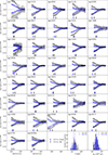 |
Fig. 2. Measured deviation of the gas-to-stellar flux ratio with respect to the galactic average as a function of the aperture sizes for each galaxy obtained by contrasting CO emission as a gas tracer respectively with Hα (black triangles) and 21 μm (blue circles) as an SFR tracer. The positive deviations correspond to measurements focusing on gas peaks (traced by CO), while the negative deviations were obtained by focusing on stellar peaks (traced respectively by Hα or 21 μm). For each data point, we also show the effective 1σ error, after the covariance between data points is taken into account. The horizontal plain line corresponding to a deviation of zero in log represents the galactic average. The dotted gray lines connecting the measurements correspond to a polynomial fit of the tuning-fork branches, following Kruijssen et al. (2018). The arrows indicate the typical separation length, λ, at which the two tracers decorrelate. The two last panels show the histograms of λ and inferred feedback timescales (tfb, defined in Section 3.3), derived for the whole sample using either Hα or 21 μm as a proxy for SFR, as well as the median and 1σ standard deviations associated with these distributions. |
The resulting “tuning-fork” shape is then fitted using two functional forms (equations 81 and 82 from Kruijssen et al. 2018), to mathematically describe the deviation of the CO-to-21 μm flux ratio from the galactic average, as a function of the aperture size, focusing on the branch associated respectively with the CO and 21 μm peaks. One specificity of the tuning-fork method lies in the fact that the latter functional form depends only on flux-weighted quantities (namely, the flux contrast between peaks and galactic averages, ℰ21 μm and ℰCO, the flux ratios between overlapping peaks and isolated peaks in both tracers, β21 μm and βCO and the enclosed flux fraction of each tracer within a given aperture size, f21 μm and fCO), making the method less sensitive to the peak identification process compared to similar approaches relying solely on the counting of emission peaks in different phases. Assuming that the emission follows a Gaussian profile centered around each of the peaks, the spacing between the two branches, their asymmetry and the inflection point, uniquely characterize a function depending on flux-related quantities, that are directly measurable on the emission maps, and of three independent parameters: the separation length between emission peaks λ, the relative duration of the isolated phase of emission (t21 μm/tCO), and the relative duration of the overlap or feedback phase (tfb, 21 μm/tCO). Other physical parameters of interest can be derived based on combinations of the latter quantities, for example the star-formation efficiency or feedback velocity, which have been previously analyzed in K22.
3.4. Reference timescale
The timescales derived following this methodology can be considered as a luminosity-weighted average of the evolutionary timeline associated with each star-forming region within a galaxy. Since we exclude galactic centers affected by blending and excessively bright peaks (see Section 3.1), these timelines represent the evolution of typical star-forming regions, located in the outer part of galaxies. Converting the relative timescales into absolute ones requires the definition of a reference timescale. In this study, we use the total cloud lifetime traced by CO(2-1) (tCO) as the reference timescale for each galaxy. The latter tCO correspond to the measurements obtained by following the exact same methodology, but contrasting maps of CO (as a tracer of the gas peaks) versus Hα as a tracer of SFR. These runs adopt the exact same set-up as the ones detailed in K22, but were updated to account for the new masks that match the field of view covered by MIRI observations (see Section 3.1). The latter runs are used to estimate the total cloud lifetime tCO, as well as the feedback timescale based on Hα (tfb, Hα).
We note that the tCO measurements are tied to a metallicity-dependent reference timescale (duration of the isolated Hα emission) calibrated in Haydon et al. (2020). This study uses the output of a hydrodynamical disk galaxy simulation combined with the stellar population synthesis model SLUG (Krumholz et al. 2015) to estimate the reference timescale associated with different observational tracers of stars, assuming a well-sample initial mass function and based on the stellar evolutionary tracks of metallicities Z/Z⊙ = 0.05, 0.20, 0.40, 2.00 (Schaller et al. 1992; Charbonnel et al. 1993; Schaerer et al. 1993a,b), where Z⊙ corresponds to the solar-metallicity. The authors report that the reference timescale corresponding to the continuum-substracted Hα varies slightly with metallicity following
![Mathematical equation: $$ \begin{aligned} t_{\rm ref}(\mathrm{H}\alpha ) [\mathrm {Myr}] = (4.32^{+0.09}_{-0.23}) \Big (\frac{Z}{Z_{\odot }} \Big )^{(-0.086^{+0.010}_{-0.023})}. \end{aligned} $$](/articles/aa/full_html/2026/02/aa56206-25/aa56206-25-eq6.gif) (2)
(2)
Within our sample spanning metallicities of 0.4Z⊙ − 1Z⊙, the Hα reference timescales vary by a factor 1.08, from 4.32 up to 4.67 Myr. This correction therefore enables accounting for a known, but moderate, metallicity-trend of the Hα visibility. The corrections introduced to account for metallicity variations are negligible compared to the uncertainties derived on our measurements. The resulting cloud lifetimes, which incorporate those metallicity variations and serve as reference timescales in the current analysis, are reported in Appendix B, Table B.1, together with the input parameters used in our analysis.
4. Results
4.1. Overview of star-formation cycle
4.1.1. Quantifying spatial decorrelations
Figure 2 shows in blue the deviation of the CO-to-21 μm flux ratio from the galactic average (Δ CO-to-21 μm), when focusing either on gas peaks in the CO maps (leading to positive Δ CO-to-21 μm) or on the 21 μm peaks (leading to negative Δ CO-to-21 μm). For comparison, we also show in black the deviations obtained when focusing on CO versus Hα peaks (Δ CO-to-Hα). We also show the analytical fits constraining the relative duration of the isolated phases and overlap phases for each pair of tracers, as well as the peaks separation lengths calculated for CO and 21 μm peaks (blue arrows) and for CO and Hα peaks (black arrows). The tuning-fork shapes associated with 21 μm are strikingly flatter than the ones derived using Hα as a tracer of SFR, in particular the top branch focusing on CO peaks. This flattening of the upper branch corresponds to a decrease of the t21 μm/tCO ratio. Most of the tuning-fork shapes also display a shift of the inflection point, corresponding to a decrease of the typical separation length λ. This indicates that the peaks of emission are typically closer in the runs involving 21 μm and CO, than when using Hα.
As described in Section 1, 21 μm and CO(2–1) both trace well molecular gas column density (see also Leroy et al. 2023b), leading to stronger correlation between CO and 21 μm. This makes the application of the statistical method described in Section 3.4 challenging, as robust timescale measurements can only be derived for galaxies where the resolution is small enough to resolve the decorrelation scale. Deriving a strict resolution threshold for all galaxies is impossible, since the decorrelation scale itself varies from galaxy to galaxy. As described in Section 2.1, our selection criterion combines both a strict cut in resolution (180 pc), corresponding to the 75% percentile of the decorrelation scale between CO and 21 μm measured in our sample, and a criterion excluding galaxies displaying flat tuning-fork branches (see Appendix B; Figure B.2). We note that the resolution threshold adopted in the current study (180 pc) is smaller than the one previously used in K22 (200 pc); this is motivated by the fact that 21 μm and CO peaks are typically closer than Hα and CO peaks, as shown by the histogram of decorrelation scales (λ) in Figure 2.
Physically, the absence of decorrelation (flat upper branch of the tuning-fork) indicates that the brightest peaks of CO emission, which dominate the flux-weighted average, are all associated with 21 μm emission. We note that this does not necessarily correspond to an absence of isolated peaks of CO emission, but only translates the fact that these isolated peaks are faint and do not contribute much to the total CO emission, compared to the ones overlapping with 21 μm. For the latter galaxies, the decorrelation between 21 μm and CO – if present – occurs at scales smaller than our working resolution. In terms of derived quantities, this corresponds to λ ≤ lap, min, which cannot be properly fitted within our statistical framework (see criterion (ii) from Appendix A). We note that Kim et al. (2025) reported similar cases of nearly flat tuning-fork branches when using PAH-tracing bands, indicating that this effect is not limited to 21 μm wavelength but might occur systematically when leveraging mid-IR tracer observed at high sensitivity. This limitation, inherent to our statistical method, is further discussed in Section 5.3.
4.1.2. Timescales associated with 21 μm emission
In this section, we report the first measurements of the timescales associated with mid-IR 21 μm emission in a large subsample of the PHANGS-JWST survey. Similar measurements were previously accessible for six galaxies only, based on the observations of Spitzer/24 μm (Kim et al. 2021) and the analysis of MIRI/21 μm for NGC 628 (Kim et al. 2023). It is now possible to carry out such analysis for a sample five times larger, for which we measure the timescales associated with the evolutionary cycle of star-forming regions, focusing in particular on the embedded feedback phase (see schematics, Figure 3). In the Appendix B, Table B.2, we report the new measurements associated with the different phases for which 21 μm emission is observable, as represented in Figure 3. The total duration associated with 21 μm emission (t21 μm), the duration of the overlap phase between CO and 21 μm (i.e., the embedded feedback associated with 21 μm emission, tfb, 21 μm), and the duration of the obscured phase of star formation is defined by
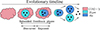 |
Fig. 3. Schematic evolutionary timeline of a star-forming region from the molecular cloud assembly until it becomes invisible in any of the three tracers we consider. In this study, we focus on the embedded feedback phase, during which stars are embedded within their host GMC. This phase is composed of an exposed phase, during which CO, 21 μm, and Hα emit simultaneously, and of an obscured phase, during which Hα emission is not detected. After the GMC dispersal, we measured an isolated phase of emission for both SFR tracers before they fade away. For most galaxies, 21 μm fades faster than Hα (upper arrow), but a few galaxies display a longer 21 μm emission (bottom arrow). |
![Mathematical equation: $$ \begin{aligned} \mathrm{t}_{\rm obscured} [\mathrm {Myr}] = \mathrm{t}_{\mathrm{fb}, 21\ \upmu \mathrm{m}} - \mathrm{t}_{\mathrm{fb, H}\alpha }, \end{aligned} $$](/articles/aa/full_html/2026/02/aa56206-25/aa56206-25-eq7.gif) (3)
(3)
where tfb, Hα corresponds to the exposed feedback phase, which is visible in optical tracers.
While we observed a decorrelation between CO and 21 μm in the 37 galaxies of our final sample, this decorrelation remains small for most of them (see Figure 2). Specifically, for 25 out of the 37 galaxies, we derived λ ≤ 1.4 × lap, min, which only enabled us to put an upper limit on the separation length, feedback timescale, and duration of the obscured star-formation phase. The temporal evolution of the assembly and dispersal of the clouds, when relying on CO and Hα observations, has been characterized previously in K22. Focusing on a subset of their sample and considering the slightly smaller field of view corresponding to the JWST coverage, we repeat the same analysis and find medians for the cloud lifetime ( Myr) and the feedback phase associated with Hα emission (
 Myr), which are in good agreement with the previous measurements for the entire sample. In Figure 4, we then combine these results with the ones presented in Table B.2 to show an overview of the entire star-formation cycle traced by CO, 21 μm and Hα. On average, we measure a total duration of the 21 μm emission of t21 μm=
  Myr (median of the measurements and of their errorbars across our sample, accounting only for the galaxies which are not affected by blending), a duration of the overlap phase between CO and 21 μm,
  Myr, and a duration of the obscured phase of star formation,
  Myr.
Myr.
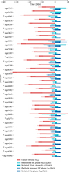 |
Fig. 4. Typical evolutionary timescales in our sample evolving from an inert CO-emitting phase to an embedded star-forming phase traced with 21 μm and eventually to an exposed star-forming phase traced with Hα emission. The feedback timescale tfb, 21 μm is an upper limit in 25 out of 37 galaxies, which are flagged with U. The upper and lower errorbars associated with each phase of the evolutionary cycle are shown as thin lines, with the same color. Galaxies are ordered by their Hubble morphological type. |
In Figure 5, we show the evolution of the feedback time derived using the 21 μm band, as a function of the feedback time measured using Hα. We confirm that the feedback time measured using a proxy sensitive to dust-embedded star formation tends to be larger than the one measured based on Hα tracing only exposed star formation. Nevertheless, we find the obscured feedback phase to be very short (≤4 Myr) in all the galaxies in our sample, with 28/37 galaxies displaying an almost absent (≤1 Myr) obscured star-formation phase. In practice, the only five galaxies (NGC 1512, NGC1433, NGC 1097, NGC 3351, and NGC 1365) where we clearly resolve a non-zero obscured phase are among the more massive, high-metallicity barred spirals (see Section 5.2.2), whereas in lower-mass systems the obscured phase is shorter than 1 Myr.
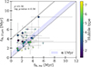 |
Fig. 5. Feedback timescale measured based on 21 μm emission versus feedback timescale measured based on Hα. The color bar shows the Hubble morphological type from the HyperLEDA database (Paturel et al. 2003a,b; Makarov et al. 2014). The dotted line shows the 1:1 relation. The obscured feedback phase traced by 21 μm (tfb, 21 μm – tfb, Hα) is less than 4 Myr in all the galaxies from our sample, as shown by the plain black line, and less than 1 Myr for 28 out of 37 galaxies, as shown by the shaded area. We display the Spearman correlation coefficient as well as the log p-value of the data, excluding upper limits. |
4.2. Environmental dependencies of the timescales
4.2.1. Selected environmental properties
We now examine how various quantities predicted by our models correlate with different galactic parameters, listed in Figure 6. In this section, we restrict our analysis to the parameters that are well constrained for all 37 galaxies from our sample (i.e., not just upper limits). We derived robust measurements in the whole sample of the total duration of the 21 μm phase, t21 μm and of the diffuse fraction of 21 μm emission, which we discuss in Sections 4.2.3 and 4.2.4. We defer the description of potential trends of λfb, 21 μm, tfb, 21 μm, and tobscured, to the discussion section (Section 5) due to the large number of upper limits.
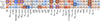 |
Fig. 6. Spearman’s rank correlation coefficients and associated p-values measured between galaxy properties (columns) and our measurements (rows). Statistically significant correlations according to the Holm-Bonferroni method (described in Section 4.2.2) are highlighted as black squares, and marginally significant correlations (log p-values < –2) are shown as blue squares. Our measurements are the total timescale of 21 μm emission (t21 μm), the ratio between timescales of SFR and gas(t21 μm/tCO), and the diffuse emission fractions of 21 μm (f |

In Figure 6, we show the Spearman rank coefficients (ρ) and the associated p-values between our predictions and numerous parameters. For the parameters that we considered, we report no strong (ρ ≥ 0.6) correlation, but there are several moderately strong (ρ ≥ 0.4) correlations, whose significance we examined based on their p-value (see Section 4.2.2). In the following, we briefly introduce the parameters considered in our analysis, which are organized in six categories.
-
Global galactic parameters. We considered global galactic properties of our sample gathered from different studies. We include the stellar masses (M*) taken from Leroy et al. (2021), the global H I mass (MHI, global) from the Lyon-Meudon Extragalactic Database (HyperLEDA; Paturel et al. 2003a,b; Makarov et al. 2014), the deviation from the main sequence (Leroy et al. 2021), and the Hubble morphological T-type from the HyperLEDA. Following K22, we also consider combinations of the later parameters, namely the global gas mass (Mgas, global = MHI, global + MH2, global), the total baryonic mass (Mtot, global = Mgas, global + M*), the molecular gas fraction (fH2, global = MH2, global/Mgas, global), the global gas mass fraction (fgas, global = Mgas, global/Mtot, global), and sSFR = SFR/M*.
-
Average kiloparsec-scale galaxy properties. We also considered kiloparsec-scale galaxy properties from Sun et al. (2022) and Sun et al. (2023). Specifically, we consider the surface densities of the SFR, atomic gas, molecular gas, and stellar mass (
 ,
,  , ΣH2kpc, and
  respectively). We also include the stellar mass volume density near the galaxy midplane (
 ) and the dynamical equilibrium pressure (P
 ), which is the pressure required to support the ISM weight (per unit area) within the gravitational potential of the galaxy (see e.g., Sun et al. 2020a). For each of the aforementioned quantity, we calculate a ΣH2kpc-weighted average per galaxy.
 -
Averaged properties of GMCs. To examine potential variations of our predictions with properties of molecular clouds, we also consider properties derived at the GMC scale for the full PHANGS–ALMA sample using the CPROPS algorithm in Rosolowsky et al. (2021) and Hughes et al. (in prep.). The latter include the velocity dispersion (σV, GMC), the virial parameter (αvir, GMC), the GMC mass (MGMC), the internal pressure (Pint), and the H2 surface density of GMCs (ΣH2, GMC). For each of these quantities, we follow the same methodology as in K22 and calculate a CO-luminosity-weighted average over the population of clouds in each galaxy.
-
Dust and ionized gas parameters. Due to the complex nature of the emission at 21 μm, we may expect dependencies not only with the parameters related to molecular gas, but also with the properties of dust and ionizing sources. For galaxies for which MUSE observations are available (20/37), we also include parameters probing the properties of the ionized gas in H II regions. For these galaxies, we consider the dust attenuation and gas-phase metallicity provided in the H II regions catalog from Groves et al. (2023). For both quantities, we consider ΣSFR-weighted average, excluding the galactic centers (as described in Section 2.3.2). Finally, we include the 50% metal-mixing scale (Lmix, 50%) from Kreckel et al. (2020) and Williams et al. (2022), a parameter that quantifies the physical scale at which the metal-mixing in the ISM is effective, using a two-point correlation function.
-
Parameters derived with HEISENBERG. We also include average properties derived by HEISENBERG within the masks described in Section 3.1. Our analysis includes the molecular gas surface density derived after the filtering of the CO maps (ΣH2, compact), the SFR surface density (ΣSFR; see Section 2.3.1), the total molecular mass associated with compact CO emission and the total SFR recalculated within the field of view of the observations. We also consider the surface density contrasts, which correspond to the flux-ratio between the average emission of the peaks and the galactic average, measured on the filtered map for CO and 21 μm respectively: ℰCO and ℰ21 μm.
-
Systematic biases. To check for the potential effects of systematic biases, we complemented the list of physical properties with some important observational features: the minimal aperture size, corresponding to the working resolution of CO observations (lap, min), which is used to convolve all maps (see Section 3.1); the inclination angle of galaxies (i) taken from Lang et al. (2020); and the mass-weighted average of CO flux completeness on kiloparsec scale (c; Sun et al. 2022), providing a metric of how deep the CO observation is. A deeper observation leads to a more complete CO flux recovery when a strict signal identification criteria is adopted.
4.2.2. Statistical framework
Following the methodology developed in Kruijssen et al. (2019a) (and also used by K22), we ranked each correlation according to their p-values for each row in Figure 6. We note that several of these correlations have p-values below the usual significance threshold (hereafter pref) of 0.05. Due to the large number of parameters considered in this study, one might expect a certain number of spurious correlations which should not be considered as significant. Hence, we further determine whether these correlations are statistically significant according to the Holm-Bonferroni method (Holm 1979). This method penalizes the second-order correlations by selecting only correlations which have a p-value below a rank-dependent threshold computed as
 (4)
(4)
where i is the rank of correlation and Ncorr the number of independent variables being evaluated. Following K22, we treat parameters with a correlation coefficient higher than 0.7 as one single variable, resulting in an estimate of Ncorr = 17.
We note that the Holm-Bonferroni method is by design relatively conservative, since it aims at narrowing the number of apparent correlations to the most significant ones. If we were to relax our significance threshold, other correlations would become significant. To account for this effect, we include in our analysis correlations which we define as “marginally significant”; the latter being associated with p-values lower than 0.01, despite not being selected through the Holm-Bonferroni method.
4.2.3. Duration of 21 μm emission
In Figure 7, we show the most significant correlations derived for the total duration of 21 μm emission, t21 μm. The left-hand panel of Figure 7 displays the evolution of t21 μm as a function of the CO luminosity-weighted average of the velocity dispersion (⟨σGMC⟩) and molecular mass of molecular clouds (⟨MGMC⟩). Both parameters correlate with t21 μm (moderately strong correlations with ρ ∼ 0.5) and are significant according to the Holm-Bonferroni method. These correlations indicate that the duration of the 21 μm emission is longer in galaxies hosting populations of massive CO-bright molecular clouds, associated with large velocity dispersion. We note that ⟨σGMC⟩ and ⟨MGMC⟩ are correlated parameters (Spearman coefficient ρ = 0.84, log p-value = −8.48), an effect which cannot be disentangled within our statistical framework. We highlight in Figure 7 the galaxies showing high surface density contrast ℰ21 μm, defined as the peak to galactic average flux ratio. Despite moderate variations of this parameter (1 ≤ ℰ21 μm ≤ 2.7), we find that the galaxies with the highest flux density contrasts tend to show enhanced duration of the 21 μm emission. We further discuss the physical mechanisms that could be responsible for this enhanced duration of 21 μm emission in Section 5.2.1.
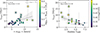 |
Fig. 7. Dependencies of the total duration of the 21 μm emitting phase (t21 μm). Left: Total duration of the 21 μm vs. CO-luminosity-weighted average velocity dispersion of GMCs. The color bar shows the CO luminosity-weighted average mass of GMCs. Galaxies with high surface density contrasts are identified with squares. We show in gray a linear regression fitted to the data and the gray-shaded area represents the 95% confidence interval on the regression, obtained with bootstrapping data. Right: Total duration of the 21 μm vs. the Hubble morphological type. The color bar shows the metallicity measurements for the galaxies observed with MUSE. |
While the Holm-Bonferroni method only selects parameters related with local properties of GMCs, we note that the total duration of 21 μm emission may also be linked to global galactic properties. In particular, the Hubble type is identified as marginally significant correlation (p-value ≤ 0.01). In the right hand-side panel of Figure 7, we show that the duration of 21 μm emission anti-correlates with the Hubble morphological type. This anti-correlation includes some significant scatter, and its analysis is complicated by the fact that standard statistical metrics do not strictly apply for discrete variables, such as the Hubble type. Nevertheless, qualitatively, we find that earlier-type galaxies hosting a bar and well-defined spiral arms, are associated with t21 μm spanning a large range of durations, up to ∼15 Myr, while later-type galaxies (less massive spirals and irregular dwarf galaxies) are associated with reduced t21 μm. We speculate that this trend may be linked to the reduced dust-content in late-type, low-metallicity environments, as we discuss further in Section 5.2.2.
In Figure 8, we examine the dependencies of the ratio of t21 μm to tCO. We note that the t21 μm/tCO is smaller than 0.5 in all galaxies in our sample apart from three, meaning that molecular clouds spend a significantly longer time (at least a factor of two) emitting CO than emitting 21 μm. As demonstrated in K22, galaxies with high molecular gas surface densities are associated with typically higher tCO. We find on the other hand that t21 μm is relatively insensitive to H2 gas surface density (weak anti-correlation with a Spearman rank coefficient of −0.3, see Figure 6). As a result, we report a significant anti-correlation of t21 μm/tCO ratios with ΣH2, compact (molecular surface density calculated after filtering out the diffuse emission), shown in Figure 8. Part of the scatter of this relation may be explained by differences in terms of atomic gas reservoir, with larger H I masses at fixed ΣH2, compact being associated with large t21 μm/tCO ratios (as shown by the color bar).
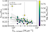 |
Fig. 8. Ratio of the total duration of the 21 μm emitting phase (t21 μm) over the total cloud lifetime (tCO) vs. H2 surface density estimated after filtering the diffuse CO emission. The color bar shows the total H I mass. |
4.2.4. Fraction of diffuse 21 μm emission
In Figure 9, we show that the fraction of diffuse emission of 21 μm (f>21 μm,diffuse) is relatively constant and comprised between 48% and 74% in our sample. These values are globally in good agreement with previous determinations reported for PHANGS-JWST Cycle 1 galaxies (Belfiore et al. 2023b; Leroy et al. 2023b; Pathak et al. 2024; Kim et al. 2025). In particular, they are similar to the ones reported in Kim et al. (2025) using the same method as in the current study for the other mid-IR bands studied in a subsample of 17 galaxies, in which they find the diffuse fraction of emission to range between 32 − 79%, 34 − 81%, and, 28 − 80% for 7.7, 10, and 11.3 μm respectively, with an average and 1σ range for f21 μm,diffuse = 62 ± 4%, very close to the value of 60 ± 10% reported in the latter study as an average for the three PAH-tracing bands.
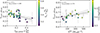 |
Fig. 9. Dependencies of the diffuse fraction of 21 μm emission (f21 μm, diffuse). Left: Diffuse fraction of 21 μm emission as a function of the global gas mass fraction. The color code shows the H2 gas mass fraction for each galaxy. Right: Diffuse fraction of 21 μm emission as a function of the kiloparsec-scale stellar surface density. The color bar shows the metallicity. |
As shown in Figure 9 (left panel), we find a significant anti-correlation of f21 μm, diffuse with the global gas fraction, mostly driven by the three galaxies with the highest gas fraction in our sample, for which f21 μm, diffuse appears clearly reduced. Focusing on the color bar, we note that the most gas-rich galaxies in our sample associated with lower fH2, may reach smaller f21 μm, diffuse values as low as ∼50%. This suggests that the contribution of diffuse 21 μm dust emission is reduced in galaxies with high gas fractions, for which the inner regions covered in our analysis are atomic-dominated (as shown by the color bar). In the right-hand side panel of Figure 9, we show that the latter gas-rich galaxies, correspond to relatively smaller stellar surface densities and lower-metallicity environments. In such galaxies, a greater share of dust heating is localized in H II regions, while more massive, dust-rich galaxies are associated with a stronger diffuse IR component.
5. Discussion
5.1. The short duration of the obscured phase of star formation
5.1.1. Comparison with previous studies using 21 μm
As described in Section 4.1.2, we found that the total duration of the 21 μm emission ranges between 1.9 and 17 Myr with a median across our sample of  Myr. We measure embedded-feedback timescales, traced by the overlap between CO and 21 μm, which are always smaller than 9 Myr, with a median of
  Myr. We find that the feedback timescales measured with 21 μm are close to the ones measured based on Hα and report a duration of the obscured star-formation phase which is ≤4 Myr in all the galaxies of our sample, with a median of
  Myr. These short timescales reinforce the idea that star formation proceeds over a relatively small fraction of the total GMC lifetime (typically, tfb, 21 μm/tCO ∼ 1/5), even when including the obscured phase of star-formation, which may limit the star-formation efficiencies in GMCs down to a few percent only (e.g., 1 − 8%, K22, Chevance et al. 2023).
This short duration of the obscured star-formation phase is consistent with previous studies focusing on the emission at 21 μm in the PHANGS-JWST sample. In particular, Hassani et al. (2023) and Hassani et al. (2025) classified > 20 000 compact 21 μm sources in the 19 first PHANGS-JWST galaxies using MIRI/21 μm data. Their results indicate that deeply embedded star-forming regions, that are faint or undetected in Hα, account for a limited fraction (≲10%) of the total 21 μm point-source population, while most of the sources are clearly associated with optical counterpart of H II regions. Our results are also consistent with the findings from Belfiore et al. (2023a) reporting that the mid-IR contamination from deeply embedded star forming region is negligible. Within the framework of our analysis, we suggest that the low number of such deeply embedded regions is representative of their very transient nature, lasting on average less than 4 Myr. We note that the value previously reported for NGC 628 in Kim et al. (2023), following the exact same methodology, falls within the range of new values reported in the current paper (tobscured = 2.3 Myr).
Myr).
These new findings made possible by JWST capabilities are consistent with previous results based on mid-IR observations performed with SPITZER/24 μm which reported small fractions of highly obscured regions without Hα counterpart (e.g., Kennicutt et al. 2003; Prescott et al. 2007; Corbelli et al. 2017). The same statistical method as the one presented in this study was also applied using 24 μm as a tracer of embedded star formation in a distinct sample of six nearby galaxies in Kim et al. (2021). The authors estimated obscured timescales of 1.4 − 3.8 Myr, in excellent agreement with the current study (0 − 3.5 Myr). We note, however, that they report a median value of tobscured = 3.0 ± 0.9 Myr, which is significantly higher than the one reported in our study, in which most galaxies are consistent with tobscured ≤ 1 Myr. Similarly, the values derived for t24 μm and tfb, 24 μm are compatible in terms of range, but with larger median values than what we measure with 21 μm. This difference between both studies is surprising, considering that the methodologies adopted in both studies are similar regarding all the aspects that could affect timescale measurements (e.g., masking schemes, filtering of diffuse emission, peak identifications, and reference timescales). Nevertheless, they may arise from biases due to different sample selection, since Kim et al. (2021) is restricted to six galaxies which are mostly lower masses (e.g., M 33, NGC 300, and LMC) and located within a maximum of 10 Mpc. We speculate that these differences could also be attributed to the significant differences in terms of sensitivity, with MIRI being up to a factor of 50 higher in terms of point-source sensitivity compared to MIPS.
5.1.2. Link with young embedded stellar populations
Short durations of the embedded phase of star formation are also measured in studies that focus on inferring molecular gas clearing timescales based on the distribution of young stellar populations. Using visual inspection of young stellar cluster (YSCs) in nearby galaxies, several studies reported that the median ages of cluster associated with dusty molecular clouds are short, of the order of 1 − 4 Myr (e.g., Whitmore et al. 2014; Calzetti et al. 2015; Hollyhead et al. 2015; Grasha et al. 2018, 2019). Similarly short gas-clearing timescales are reported by studies classifying YSCs based on the Hα morphology of their surrounding H II regions (Hannon et al. 2019, 2022). These gas- and dust-clearing timescales are sensitive to the tracers used to select YSCs; in particular it has been suggested that accounting for the deeply embedded clusters which are only visible in the near-IR could enhance the duration of the embedded phase with respect to measurements based on optical and UV tracers only. The population of embedded clusters, which are missed in the optical, have been shown to represent up to 10 − 15% of the cluster populations in well-studied nearby galaxies (e.g., Whitmore & Zhang 2002; Whitmore et al. 2023, 2025).
Whether this population of previously missed IR clusters significantly enhance the measured embedded timescales remain to be elucidated. Focusing on IR-selected clusters based on Hubble/F336W in M83, Deshmukh et al. (2024) measured equally short clearing timescales as in previous studies with 75% of their IR-selected sources having a dust attenuation AV < 1 by 2 Myr, and 82% by 3 Myr. On the other hand, Messa et al. (2021) report clearing timescales that are ∼1 Myr longer than previously estimated In NGC 1313 based on near-UV-optical cluster studies. Similarly, in the dwarf galaxy NGC 4449, McQuaid et al. (2024) recently measured slightly higher clearing timescales (5–6 Myr) and smaller median cluster mass (∼7 × 10³ M⊙) than the values reported for UV/optical catalogs (5 Myr, and ∼3.5 × 10⁴ M⊙). They interpret these differences as evidence that clearing timescales depend on the cluster mass, due to reduced efficiency of both pre-supernova and supernovae feedback in lower mass clusters, that can only be probed in the IR.
Complementing these studies, the recent JWST observations enable measurements of the emergence timescale of young stellar clusters via numerous independent techniques, including statistics on different classes of objects, age estimates derived by fitting the spectral energy distributions (SEDs), and age-dating with Paα equivalent width. Despite differences in the methodologies adopted in different studies, the reported embedded timescales appear consistently short (≲5 Myr) across different types of environments (e.g., Sun et al. 2024; Whitmore et al. 2023; Linden et al. 2024; Pedrini et al. 2024; Rodríguez et al. 2025; Knutas et al. 2025; Graham et al. 2025). These age estimates are in globally good agreement with the embedded feedback timescales reported in our study (with a median across our sample of  Myr). We note that our luminosity-weighted method bias our results toward the more massive star-forming regions, that may not be representative of the evolution timeline associated with clusters of smaller masses. Recently, Knutas et al. (2025) reported evidence that the emergence of massive star cluster (> 5 × 10³ M⊙) is ∼2 Myr shorter than for cluster of masses ∼103 M⊙ in M 83.
The mid-IR 3.3 μm emission has also been used to trace the survival timescale of PAHs in the earliest star-formation phase, corresponding to our dust-obscured feedback phase. Recent studies report that PAH emission fades within ∼3–4 Myr, consistent with the picture of a very transient obscured star-formation phase (Linden et al. 2024; Rodríguez et al. 2025; Knutas et al. 2025; Whitmore et al. 2025). Focusing on NGC 628, Whitmore et al. (2025) compared the SEDs of nearly embedded cluster candidates (strong PAH and continuum emitters with a faint optical counterpart) from Rodríguez et al. (2025) and Hassani et al. (2023) to empirical based SED template based on optically identified clusters, and found that their IR SED closely resemble that of optically selected cluster with age 1 to 3 Myr. Focusing on the 12 nearly embedded clusters from Hassani et al. (2023) identified with large-aperture photometry at 21 μm, the authors report an age of about 1 Myr, younger than most of their optically selected clusters and in good agreement with the dust-obscured timescales that we derive in the current study.
5.2. Parameters affecting the emission of 21 μm
5.2.1. Impact of the average GMC properties
As previously discussed in Section 4.2, the total duration of the 21 μm emission, t21 μm is relatively insensitive to global galactic parameters (e.g., SFR, gas and star masses, and surface densities). On the other hand, we find that among the moderately strong correlations of identified in Section 4.2.3, the most significant correlation is with the CO luminosity-weighted average of local properties of GMCs measured at 150 pc, in particular the velocity dispersion and mass of GMCs (see Figure 6). Despite the numerous upper limits, we show on Figure 10 that the feedback timescale measured based on 21 μm also seem to increase with increasing velocity dispersion and mass of GMCs (the table of correlations derived for these 12 measurements is provided in Appendix B; Figure B.3).
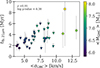 |
Fig. 10. Duration of the feedback time (tfb, 21 μm) as a function of the CO luminosity-weighted average velocity dispersion of molecular clouds. The color bar shows the CO luminosity-weighted average mass of GMCs. |
Although we find that t21 μm, and tentatively tfb, 21 μm, correlate best with GMC mass and velocity dispersion, these GMC properties themselves correlate with galaxy-scale quantities (stellar mass, molecular gas mass, SFR gas surface density, as well the mid-plane dynamical equilibrium pressure; Sun et al. 2022). Thus, what we are really seeing could be a reflection of high-pressure environments (found in massive galaxies or galaxy centers) yielding both more massive GMCs and slightly longer embedded phases.
The latter correlations with physical properties of GMCs have important implications for high-redshift galaxies, which host populations of higher-pressure GMCs with higher velocity dispersion (e.g., Claeyssens et al. 2023) and masses up to ∼100 times larger at z ∼ 1 (e.g., Dessauges-Zavadsky et al. 2019, 2023). Such GMCs are the likely progenitors of globular clusters (e.g., Kruijssen 2026). Our results suggest that in such environments, both the total duration of the 21 μm emission and the feedback timescales could be increased, as star formation may proceed over a longer period before the molecular clouds are disrupted. This result also indicates that the short GMC surviving timescale and rapid cycling of matter derived for nearby galaxies may only hold for nearby galaxies but should be revised for any galaxies in which we expect a significantly different population of molecular clouds. We note, however, that the timescales associated with 21 μm emission do not directly reflect the presence/disruption of gas and dust, but that the observed 21 μm reflects the coupling of dust grains with UV radiation fields. As a result, it may be difficult to make predictions for environments where we expect both the dust properties and heating mechanisms to vary.
Disentangling the underlying physical mechanisms responsible for the emission of a given tracer is not easy with observations. State-of-the-art simulations, such as STARFORGE (Grudić et al. 2021), that implement various stellar feedback mechanisms can provide a complementary view on the evolutionary cycle at GMC scales. Using STARFORGE simulation, post-processed in the mid-IR (e.g., 24 μm), Wainer et al. (2025) examine the embedded phase of star formation and its observational signatures. Their predicted timescales are in good agreement with the measurements of a few Myr from the current study, indicating that the physical mechanisms implemented in their simulations are compatible with what is probed observationally in nearby galaxies. Interestingly, the authors also report an increased duration of the embedded phase with the cloud free fall time. They attribute this scaling with free fall time to the longer build-up timescales for massive stars in higher-mass GMCs. While a detailed comparison between our observationally based approach and GMC-scale simulations remains to be further explored, this effect provides a possible physical interpretation for the tobscured versus ⟨MGMC⟩ reported in the current study.
5.2.2. Impact of morphological type and metallicity
Previous studies have shown that the frequency of regions in different evolutionary stages vary with the morphological type of galaxies (e.g., Pan et al. 2022). Understanding the physical drivers of such differences is complicated by the fact that the morphological type of galaxies strongly correlates with other global parameters, and in particular with the stellar mass and the metallicity, which both decrease in later-type objects. Pan et al. (2022) report that the barred spiral galaxies, corresponding the earliest Hubble T-type in our sample, are associated with a large reservoir of CO-emitting gas, unassociated with Hα emission, while later type galaxies exhibit more H II regions, associated with low-mass or partially dispersed molecular clouds. The authors report a correlation of the Hubble type with the fraction of sight-lines showing Hα only emission and an anti-correlation with the fraction of sight-lines showing CO emission, at 150 pc. They also report a moderate increase of the fraction of regions where both CO and Hα overlap, for later type galaxies. While the exact numerical details differ from our statistical approach, their results should translate into correlations in terms of CO and Hα timescales. Specifically, one might expect a longer tCO, as well a shorter tfb, Hα in early-type galaxies. This anti-correlation is indeed reported in K22, although it is not identified as significant. Nevertheless, both studies remain in good agreement, indicating that longer tCO timescales are expected in earlier-type and higher-mass galaxies.
In the current study, we find a moderate anti-correlation (Spearman coefficient = 0.46, log p-value = −2.36) between the Hubble type and the total duration of the 21 μm emission (see Figure 7). Although this anti-correlation is classified as marginally significant within our statistical framework, it is one of the most significant among the parameters we examined and has a lower p-value than the correlations with the total gas mass and stellar mass. We suggest that the increase of t21 μm observed in massive, early-type galaxies may be driven by metallicity effects, as shown by the color bars from Figure 7. This result indicates that the total duration of the 21 μm emission, seen before and after GMC dispersal, is longer in early type galaxies associated with higher dust-content. In particular, we note that the five barred spiral galaxies showing clear non-zero obscured star-formation phase are associated with significantly longer isolated phase of 21 μm emission, that remain visible for more than 4 Myr after GMC dispersal (see Figure 4).
In Figure 11 (left), we further investigate tentative correlations between the duration of the obscured star-formation phase and the Hubble type and metallicity. Despite a small dynamical range in the y-axis, and numerous upper limits, we report a tentative anti-correlation between tobscured and the Hubble type, indicating that in earlier type barred galaxies, associated with higher metal and dust content the newly born stars may stay enshrouded in dusty molecular clouds for a relatively longer time. While a robust confirmation of such claims would require a larger number of galaxies, we further examine possible trends of the timescales associated with 21 μm as a function of metallicity, for 20/37 galaxies for which metallicity measurements with MUSE are available. Focusing on the outer part of the galaxies (i.e., masking galactic centers) leads to average gas-phase metallicities that are below the solar-value for all galaxies, going from 12+log(O/H) = 8.60±0.01 in NGC 3351 down to 8.29 ± 0.003 in NGC 5068. The latter metallicities also cover a slightly larger range of values than when using a simple mass-metallicity relation, but still somewhat limited (∼0.4 dex). We stress that the range of metallicities probed within the PHANGS sample remains limited, with only two data points at low-metallicity (NGC 5068 with 12+log(O/H) = 8.29±0.003 and NGC 4731 with 12+log(O/H) = 8.29±0.04).
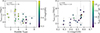 |
Fig. 11. Dependencies of the duration of the obscured star-formation time (tobscured). Left: Duration of the obscured star-formation time as a function of the morphological type of galaxies from the HyperLEDA database (Paturel et al. 2003a,b; Makarov et al. 2014). The color bar shows the gas-phase metallicity measured with MUSE. Right: Duration of the obscured star-formation phase (bottom) as a function of gas-phase metallicity. The color bar shows the evolution of the SFR surface density. |
For ten out of 20 of these galaxies, we derive only upper limits for tfb, 21 μm, tobscured, and λfb, 21 μm. As shown in Figure 11 (right), for this subsample of galaxies we find a strong correlation (ρ = 0.89, p-value = –3.21) between tobscured and the gas phase metallicity. Similarly, we found correlations of t21 μm ((ρ = 0.54, p-value = –1.87) and tfb, 21 μm (ρ = 0.77, p-value = –2.05) with metallicity. These correlations with metallicity may reflect a change in the dust-to-gas mass ratio, which is known to evolve with metallicity (e.g., Reémy-Ruyer et al. 2014; Galliano et al. 2021; Méndez-Delgado et al. 2024), with potentially a strong impact on the population of small grains which power 21 μm emission. The increased feedback timescales as a function of metallicity may also indicate that feedback by massive stellar winds, which becomes stronger with metallicity, is not responsible for the emergence of young stellar population from CO clouds, which could instead be driven by photoionization feedback mechanisms. In the low-metallicity regime probed by dwarf galaxies (1/2 Z⊙–1/10 Z⊙), changes in terms of gas morphology are expected under the effect of photoionization, leading to an increased porosity of the interstellar medium to UV photons (e.g., Cormier et al. 2019; Polles et al. 2019; Madden et al. 2020; Chevance et al. 2020b; Lebouteiller & Ramambason 2022; Ramambason et al. 2022). While the metallicity range probed by our current sample is higher, an increased porosity among the lowest metallicity object would be qualitatively consistent with a reduced duration of the obscured timescale when metallicity decreases.
Theoretical studies have also shown that the physical mechanisms regulating the cloud assembly and destruction may significantly be affected by metallicity. In Fukushima et al. (2020), the authors perform 3D radiation hydrodynamical (RHD) simulations with varying metallicity (1, 1/10, and 1/100 Z ⊙) and report that the star-formation efficiency is systematically reduced with decreasing metallicity (by a factor ∼2 at a metallicity of 1/10 Z⊙ and ∼3 at a metallicity of 1/100 Z⊙, compared to the solar metallicity case), regardless of the initial surface density of the clouds. In addition, the authors report a faster expansion of H II region that disrupt the molecular clouds in shorter timescales. Similarly, Yoo et al. (2020) perform RHD simulation of molecular clouds with varying metallicity and calculated that the “enshrouded” time during which the stars remained fully embedded in their birth cloud is on average reduced in their low metallicity runs, going from ∼4 Myr at solar metallicity down to 2.4 Myr on average at ∼1/10 Z⊙. Both the values and the tentative trends that we report in this section are qualitatively consistent with these predictions.
5.3. Limitations and future improvements
One of the main limitation of the current study is the limited resolution and sensitivity of the molecular gas tracer (ALMA/CO(2-1)) compared to the one of the MIRI/21 μm. The high sensitivity of the mid-IR observations leads to the detection of more peaks of emission than when using ground-based Hα as a tracer of star formation (e.g., in K22). The average decorrelation scale between CO and 21 μm, λ21 μm, is systematically smaller than the average separation length measured between CO and Hα, as shown by the histogram in Figure 2. While this higher sensitivity is not a limitation in itself, it causes most of the galaxies in our sample to break one of the validity criteria of our statistical method (see item (ii) from Appendix A), specifically the requirement that the decorrelation scale must be at least 1.4 times larger than the working resolution for the derived estimates of λ and tfb to be robust. Since 25 out of 37 galaxies in our sample are best fitted with a λ value smaller than ∼1.4 times the minimum aperture (fixed by the resolution of CO maps), only upper limits can be derived for λfb, 21 μm and tfb, 21 μm (Kruijssen et al. 2018).
In addition to this first observational limitation, there is a mismatch of a factor of ∼2 between 21 μm and CO(2–1) sensitivities (see criterion number (vi) from Appendix A). Indeed, using the 5σ sensitivity of the CO maps (∼105 M⊙; Leroy et al. 2021) and the integrated star-formation efficiencies calculated in K22, we estimate a minimal young stellar mass probed by CO observations ranging from 800 M⊙ to 8000 M⊙, with a median value of ∼3600 M⊙. Instead, the minimal young stellar mass which is probed with the 21 μm observation is ∼1500 M⊙, two times smaller than the values obtained with CO maps (see Appendix A for the detailed calculation). This indicates that the young stellar populations probed in the 21 μm maps may not be detectable with the current sensitivity of our molecular gas tracer. Effectively, this could bias our results toward measuring relatively longer timescales associated with 21 μm emission. We note that this effect does not affect the conclusions from our study, since most measurements are already upper limits due to the resolution issue mentioned previously. However, it is important to stress that converting the upper limits from the current study into actual measurements would require matching both the resolution and the sensitivity of the SFR and molecular gas tracers.
One possible avenue to solve this issue would be to use another proxy to probe the neutral gas reservoir, obtained at a higher angular resolution and sensitivity. Falling into the range of detection of JWST imagers, PAH bands have been shown to be good tracers of cold neutral gas distribution (e.g., Whitcomb et al. 2023; Chown et al. 2025), making them interesting proxies of cold gas at higher spatial resolution than CO. Nevertheless, their complex origin influenced by the ISM distribution, radiation, and abundances of dust and PAHs, complicate the interpretation of their spatial variations, in particular near H II regions where PAHs may be destroyed (e.g., Chastenet et al. 2023; Egorov et al. 2023; Sutter et al. 2024). Other spectroscopic tracers, such as the vibrationally excited H2 lines, only probe a partial, warmer, H2 gas reservoir and their observability is strongly limited by the small field of view of JWST spectrometers. As a result, no tracer other than CO is currently available to trace the bulk molecular gas distribution.
A detailed analysis contrasting the mid-IR PAHs bands with MUSE/Hα observations has recently been carried out in Kim et al. (2025). Nevertheless, using mid-IR bands to trace both the gas reservoirs (via PAH-dominated bands or H2) and the SFR (via 21 μm) would bring additional challenges regarding the timeline calibration and the interpretation of the timescales. A first difficulty would be to define a reference timescale associated with the emission of at least one tracer, which is a necessary step to convert the relative timescales derived in HEISENBERG into absolute timescales (see Section 3.4). Another challenge is to interpret the timescales associated with tracers which may be only probing part of the star-forming molecular gas reservoirs. Indeed, one important assumption of the statistical approach used here is that the compact emission of the selective tracers used in the analysis traces well the gas that has formed or will form stars.
While the analysis presented in this study relies on classical tracers of molecular gas and SFR, the timescales we derive are also sensitive to how well our selected tracers spatially agree with the underlying distribution of gas and stars. In particular, the interpretation of the timescales associated with the total cloud lifetime and feedback time would be complicated if mechanisms other than stellar feedback are causing the decorrelation between the gas and SFR tracers (e.g., drift of GMCs, ionizing photons leaking out of star-formation sites, runaway stars; Koda & Tan 2023; Hu et al. 2024). If present, dynamical drift effects and Hα diffusion effects would both likely lead to an underestimation of the cloud lifetime. Disentangling the signatures associated with these various scenarios remains challenging and requires access to observations at higher spatial resolution than currently accessible in the PHANGS survey (below ∼50 pc in both Hα and CO(1–0), only achieved in NGC 628 and NGC 5068). In a recent analysis including the two latter galaxies, Kruijssen et al. (2024) have shown that a decorrelation arising solely from the dynamical drift of GMCs is statistically unlikely with respect to the feedback-driven hypothesis, in all the galaxies with sufficient spatial resolution to allow this test to be performed.
In addition, the presence of CO-dark H2 gas, undetected in CO(2–1) may also bias our timescale estimates toward smaller cloud lifetimes. This effect has recently been quantified in Kim et al. (2025) and was found to be negligible for most galaxies from the PHANGS sample, which have a metallicity close to the solar value. Significant underestimations of the cloud lifetimes traced by CO are only expected in galaxies associated with low-metallicity (Ward et al. 2020, 2022; Kim et al. 2025). As a result, extending our analysis to a sample including low-metallicity dwarf galaxies may become challenging, since CO molecules do not self-shield as effectively as H2, making it notoriously difficult to detect at low metallicity (e.g., Madden et al. 2020). Nevertheless, in order to confirm the potential trends of t21 μm, tfb, 21 μm, and tobscured with metallicity discussed in the current paper (see Section 5.2.2), including galaxies that probe the lower metallicity regime is crucially needed.
The timescales we derive here, similar to all the previous work relying on a similar statistical method, are representative of the average timescale of molecular clouds. While the measured uncertainties account for both internal variations within galaxies and systematic effects, the measurements themselves represent luminosity-weighted averages, integrated on galactic scales. In the current paper, we find that evolutionary timescales of GMCs depend on the interplay between the chemical properties of galaxies (metallicity and dust content), the gas distribution of star-forming gas reservoirs (morphological type and masses of GMCs), as well as on the physical mechanisms injecting energy at the scale of GMCs and controlling the velocity dispersion of GMCs. To disentangle these complex multiscale effects, studying the internal variations of GMCs within the same galaxy is essential. In particular, a promising avenue consists in examining how local environmental variations may affect the derived timelines (e.g., arm versus interarm regions; Romanelli et al. 2025) and how these timescales may evolve radially, from the centers to the outer edges of galaxies (e.g., Kruijssen et al. 2019b; Chevance et al. 2020b; Ward et al. 2020, 2022, Romanelli et al. in prep.). Such studies are necessary to probe the impact of the local ISM properties on the derived timescales and assess the potential role of galactic dynamics in GMCs evolution.
6. Conclusion
In this paper, we have analyzed a sample of 37 nearby star-forming galaxies observed in a wide range of wavelengths as part of the PHANGS surveys. We combined ALMA/CO(2-1), ground-based Hα, and JWST/21 μm observations in order to constrain the evolutionary cycle of molecular clouds, including the dust-embedded star-formation phase. We analyzed the spatial correlations and decorrelations between CO and 21 μm maps after filtering the diffuse emission present in both maps and masking the central regions affected by blending. We then used the HEISENBERG code to convert these spatial offsets into timescales associated with 21 μm emission. Our main findings are summarized below:
-
Across the sample considered in our analysis and excluding galaxies affected by blending, we measured a median total duration of 21 μm emission of
 Myr, an embedded feedback timescale associated with 21 μm emission of
  Myr, and an obscured phase of star formation of
  Myr. We find that the obscured phase of star formation, which is not visible in Hα, is short in all the galaxies from our sample, lasting a maximum of 4 Myr, and is less than 1 Myr in 28 out of 37 galaxies.
 -
We examined the correlations of the timescales we derived with numerous parameters that include galaxy-integrated properties, average kiloparsec-scale properties, average GMC properties, properties of the ionized gas and dust, measurements with HEISENBERG, and systematic biases. We find moderately strong but statistically significant correlations of the total emission time of t21 μm with the mass and velocity dispersion of GMCs. We also identified marginally significant correlations of t21 μm with the Hubble morphological type, which may reflect an impact of the gas-phase metallicity.
-
We measured a fraction of diffuse emission contribution to the emission of 21 μm, which is relatively constant throughout our sample, in the range of 48 − 74%, with a median value of 62 ± 4%. This fraction of diffuse emission correlates best with the global gas mass fraction, the molecular gas mass fraction, and the kiloparsec-scale stellar surface density, and to a lesser extent it correlates with the properties of GMCs (mass and velocity dispersion).
-
We discussed the potential trend of the feedback timescale (tfb, 21 μm) and the embedded phase of star formation (tobscured) with various parameters. We find that tfb, 21 μm may be sensitive to changes in the GMCs properties, in particular variations of the mass and velocity dispersion of the population of clouds that dominate the emission. On the other hand, tobscured appears to be sensitive to the morphological type of galaxies, with barred spiral galaxies showing a longer obscured phase of star formation (∼4 Myr), while low-mass flocculent spiral and irregular galaxies show a reduced duration of the embedded phase of star formation.
-
Finally, we examined potential trends of the timescales associated with 21 μm with metallicity and find that t21 μm, tfb, 21 μm, and tobscured tend to increase with metallicity, which could be due to the effect of a higher dust-to-gas mass ratio. If this trend is confirmed, it would favor the dispersal of dust and CO clouds through ionization feedback mechanisms rather than feedback from stellar winds, which is instead expected to increase with metallicity. Extending the parameter space probed in this study to the low-metallicity regime is necessary to confirm the presence of such trends.
Acknowledgments
We thank the anonymous referee for constructive comments that significantly improved the clarity of our manuscript. This work was carried out as part of the PHANGS collaboration. LR, MC, and AR gratefully acknowledge funding from the DFG through an Emmy Noether Research Group (grant number CH2137/1-1). COOL Research DAO (Chevance et al. 2025) is a Decentralized Autonomous Organization supporting research in astrophysics aimed at uncovering our cosmic origins. J.K. is supported by a Kavli Fellowship at the Kavli Institute for Particle Astrophysics and Cosmology (KIPAC). HAP acknowledges support from the National Science and Technology Council of Taiwan under grant 113-2112-M-032-014-MY3. JS acknowledges support by the National Aeronautics and Space Administration (NASA) through the NASA Hubble Fellowship grant HST-HF2-51544 awarded by the Space Telescope Science Institute (STScI), which is operated by the Association of Universities for Research in Astronomy, Inc., under contract NAS 5-26555. MB acknowledges support by the ANID BASAL project FB210003. This work was supported by the French government through the France 2030 investment plan managed by the National Research Agency (ANR), as part of the Initiative of Excellence of Université Côte d’Azur under reference No. ANR-15-IDEX-01. This research was funded, in whole or in part, by the French National Research Agency (ANR), grant ANR-24-CE92-0044 (project STARCLUSTERS). We thank the German Science Foundation DFG for financial support in the project STARCLUSTERS (funding ID KL 1358/22-1 and SCHI 536/13-1). OE acknowledges funding from the Deutsche Forschungsgemeinschaft (DFG, German Research Foundation) – project-ID 541068876. SCOG acknowledges financial support from the European Research Council via the ERC Synergy Grant “ECOGAL” (project ID 855130) and from the German Excellence Strategy via the Heidelberg Cluster of Excellence (EXC 2181 – 390900948) “STRUCTURES”. KK gratefully acknowledges funding from the Deutsche Forschungsgemeinschaft (DFG, German Research Foundation) in the form of an Emmy Noether Research Group (grant number KR4598/2-1, PI Kreckel) and the European Research Council’s starting grant ERC StG-101077573 (“ISM-METALS”). This work is based on observations made with the NASA/ESA/CSA JWST. The data were obtained from the Mikulski Archive for Space Telescopes at the Space Telescope Science Institute, which is operated by the Association of Universities for Research in Astronomy, Inc., under NASA contract NAS5-03127. The observations are associated with JWST programs 2107 and 3707. The specific observations analyzed can be accessed via https://doi.org/10.17909/ew88-jt15. This paper includes data gathered with the 2.5 meter du Pont located at Las Campanas Observatory, Chile, and data based on observations carried out at the MPG 2.2m telescope on La Silla, Chile. Based on observations collected at the European Southern Observatory under ESO programs 0111.C-2109 (PI: Egorov), 0108.B-0249 (PI: Kreckel), 094.C-0623 (PI: Kreckel), 095.C-0473, 098.C-0484 (PI: Blanc), 1100.B-0651 (PHANGS-MUSE; PI: Schinnerer), as well as 094.B-0321 (MAGNUM; PI: Marconi), 099.B-0242, 0100.B-0116, 098.B-0551 (MAD; PI: Carollo) and 097.B-0640 (TIMER; PI: Gadotti). This paper makes use of the following ALMA data, which have been processed as part of the PHANGS–ALMA survey: ADS/JAO.ALMA#2012.1.00650.S, ADS/JAO.ALMA#2013.1.01161.S, ADS/JAO.ALMA#2015.1.00925.S, ADS/JAO.ALMA#2015.1.00956.S, ADS/JAO.ALMA#2017.1.00392.S, ADS/JAO.ALMA#2017.1.00886.L, ADS/JAO.ALMA#2018.1.01651.S. ALMA is a partnership of ESO (representing its member states), NSF (USA) and NINS (Japan), together with NRC (Canada), MOST and ASIAA (Taiwan), and KASI (Republic of Korea), in cooperation with the Republic of Chile. The Joint ALMA Observatory is operated by ESO, AUI/NRAO and NAOJ. This paper includes data gathered with the 2.5 meter du Pont located at Las Campanas Observatory, Chile, and data based on observations carried out at the MPG 2.2m telescope on La Silla, Chile. This paper used the following software packages : Astropy (Astropy Collaboration 2013, 2018, 2022), Clumpfind (Williams et al. 1994), Heisenberg (Kruijssen et al. 2018), Matplotlib (Hunter 2007), SciPy (Virtanen et al. 2020), seaborn (Waskom 2021), pandas (McKinney 2010).
References
- Accurso, G., Saintonge, A., Catinella, B., et al. 2017, MNRAS, 470, 4750 [NASA ADS] [Google Scholar]
- Adamo, A., Ryon, J. E., Messa, M., et al. 2017, ApJ, 841, 131 [Google Scholar]
- Aniano, G., Draine, B. T., Gordon, K. D., & Sandstrom, K. 2011, PASP, 123, 1218 [Google Scholar]
- Asplund, M., Grevesse, N., Sauval, A. J., & Scott, P. 2009, ARA&A, 47, 481 [NASA ADS] [CrossRef] [Google Scholar]
- Astropy Collaboration (Robitaille, T. P., et al.) 2013, A&A, 558, A33 [NASA ADS] [CrossRef] [EDP Sciences] [Google Scholar]
- Astropy Collaboration (Price-Whelan, A. M., et al.) 2018, AJ, 156, 123 [Google Scholar]
- Astropy Collaboration (Pedregosa, F., et al.) 2022, ApJ, 935, 167 [NASA ADS] [CrossRef] [Google Scholar]
- Belfiore, F., Santoro, F., Groves, B., et al. 2022, A&A, 659, A26 [NASA ADS] [CrossRef] [EDP Sciences] [Google Scholar]
- Belfiore, F., Leroy, A. K., Sun, J., et al. 2023a, A&A, 670, A67 [NASA ADS] [CrossRef] [EDP Sciences] [Google Scholar]
- Belfiore, F., Leroy, A. K., Williams, T. G., et al. 2023b, A&A, 678, A129 [NASA ADS] [CrossRef] [EDP Sciences] [Google Scholar]
- Bigiel, F., Leroy, A., Walter, F., et al. 2008, AJ, 136, 2846 [NASA ADS] [CrossRef] [Google Scholar]
- Blanc, G. A., Heiderman, A., Gebhardt, K., Evans, N. J., II, & Adams, J. 2009, ApJ, 704, 842 [NASA ADS] [CrossRef] [Google Scholar]
- Bolatto, A. D., Wolfire, M., & Leroy, A. K. 2013, ARA&A, 51, 207 [CrossRef] [Google Scholar]
- Bonne, L., Kabanovic, S., Schneider, N., et al. 2023, A&A, 679, L5 [NASA ADS] [CrossRef] [EDP Sciences] [Google Scholar]
- Calzetti, D., Kennicutt, R. C., Engelbracht, C. W., et al. 2007, ApJ, 666, 870 [Google Scholar]
- Calzetti, D., Johnson, K. E., Adamo, A., et al. 2015, ApJ, 811, 75 [CrossRef] [Google Scholar]
- Charbonnel, C., Meynet, G., Maeder, A., Schaller, G., & Schaerer, D. 1993, A&AS, 101, 415 [NASA ADS] [Google Scholar]
- Chastenet, J., Sutter, J., Sandstrom, K., et al. 2023, ApJ, 944, L11 [NASA ADS] [CrossRef] [Google Scholar]
- Chevance, M., Kruijssen, J. M. D., Hygate, A. P. S., et al. 2020a, MNRAS, 493, 2872 [NASA ADS] [CrossRef] [Google Scholar]
- Chevance, M., Kruijssen, J. M. D., Vazquez-Semadeni, E., et al. 2020b, Space Sci. Rev., 216, 50 [NASA ADS] [CrossRef] [Google Scholar]
- Chevance, M., Kruijssen, J. M. D., Krumholz, M. R., et al. 2022, MNRAS, 509, 272 [Google Scholar]
- Chevance, M., Krumholz, M. R., McLeod, A. F., et al. 2023, ASP Conf. Ser., 534, 1 [NASA ADS] [Google Scholar]
- Chevance, M., Kruijssen, J. M. D., & Longmore, S. N. 2025, ArXiv e-prints [arXiv:2501.13160] [Google Scholar]
- Chown, R., Leroy, A. K., Sandstrom, K., et al. 2025, ApJ, 983, 64 [Google Scholar]
- Claeyssens, A., Adamo, A., Richard, J., et al. 2023, MNRAS, 520, 2180 [NASA ADS] [CrossRef] [Google Scholar]
- Colombo, D., Hughes, A., Schinnerer, E., et al. 2014, ApJ, 784, 3 [NASA ADS] [CrossRef] [Google Scholar]
- Congiu, E., Blanc, G. A., Belfiore, F., et al. 2023, A&A, 672, A148 [NASA ADS] [CrossRef] [EDP Sciences] [Google Scholar]
- Cook, D. O., Lee, J. C., Adamo, A., et al. 2019, MNRAS, 484, 4897 [NASA ADS] [CrossRef] [Google Scholar]
- Corbelli, E., Braine, J., Bandiera, R., et al. 2017, A&A, 601, A146 [NASA ADS] [CrossRef] [EDP Sciences] [Google Scholar]
- Cormier, D., Abel, N. P., Hony, S., et al. 2019, A&A, 626, A23 [NASA ADS] [CrossRef] [EDP Sciences] [Google Scholar]
- de los Reyes, M. A. C., & Kennicutt, R. C. Jr. 2019, ApJ, 872, 16 [NASA ADS] [CrossRef] [Google Scholar]
- den Brok, J. S., Chatzigiannakis, D., Bigiel, F., et al. 2021, MNRAS, 504, 3221 [NASA ADS] [CrossRef] [Google Scholar]
- Deshmukh, S., Linden, S. T., Calzetti, D., et al. 2024, ApJ, 974, L24 [Google Scholar]
- Dessauges-Zavadsky, M., Richard, J., Combes, F., et al. 2019, Nat. Astron., 3, 1115 [NASA ADS] [CrossRef] [Google Scholar]
- Dessauges-Zavadsky, M., Richard, J., Combes, F., et al. 2023, MNRAS, 519, 6222 [NASA ADS] [CrossRef] [Google Scholar]
- Egorov, O. V., Kreckel, K., Sandstrom, K. M., et al. 2023, ApJ, 944, L16 [NASA ADS] [CrossRef] [Google Scholar]
- Emsellem, E., Schinnerer, E., Santoro, F., et al. 2022, A&A, 659, A191 [NASA ADS] [CrossRef] [EDP Sciences] [Google Scholar]
- Engargiola, G., Plambeck, R. L., Rosolowsky, E., & Blitz, L. 2003, ApJS, 149, 343 [NASA ADS] [CrossRef] [Google Scholar]
- Espinosa-Ponce, C., Sánchez, S. F., Morisset, C., et al. 2020, MNRAS, 494, 1622 [Google Scholar]
- Evans, N. J., II, Dunham, M. M., Jørgensen, J. K., et al. 2009, ApJS, 181, 321 [Google Scholar]
- Fujimoto, Y., Chevance, M., Haydon, D. T., Krumholz, M. R., & Kruijssen, J. M. D. 2019, MNRAS, 487, 1717 [NASA ADS] [CrossRef] [Google Scholar]
- Fukushima, H., Yajima, H., Sugimura, K., et al. 2020, MNRAS, 497, 3830 [Google Scholar]
- Galliano, F., Nersesian, A., Bianchi, S., et al. 2021, A&A, 649, A18 [EDP Sciences] [Google Scholar]
- Graham, G. B., Dale, D. A., Smith, C. L., et al. 2025, AJ, 170, 340 [Google Scholar]
- Grasha, K., Calzetti, D., Bittle, L., et al. 2018, MNRAS, 481, 1016 [NASA ADS] [CrossRef] [Google Scholar]
- Grasha, K., Calzetti, D., Adamo, A., et al. 2019, MNRAS, 483, 4707 [NASA ADS] [CrossRef] [Google Scholar]
- Gratier, P., Braine, J., Rodriguez-Fernandez, N. J., et al. 2010, A&A, 522, A3 [NASA ADS] [CrossRef] [EDP Sciences] [Google Scholar]
- Gratier, P., Braine, J., Rodriguez-Fernandez, N. J., et al. 2012, A&A, 542, A108 [NASA ADS] [CrossRef] [EDP Sciences] [Google Scholar]
- Groves, B., Kreckel, K., Santoro, F., et al. 2023, MNRAS, 520, 4902 [Google Scholar]
- Grudić, M. Y., Guszejnov, D., Hopkins, P. F., Offner, S. S. R., & Faucher-Giguère, C.-A. 2021, MNRAS, 506, 2199 [NASA ADS] [CrossRef] [Google Scholar]
- Hannon, S., Lee, J. C., Whitmore, B. C., et al. 2019, MNRAS, 490, 4648 [NASA ADS] [CrossRef] [Google Scholar]
- Hannon, S., Lee, J. C., Whitmore, B. C., et al. 2022, MNRAS, 512, 1294 [NASA ADS] [CrossRef] [Google Scholar]
- Hassani, H., Rosolowsky, E., Leroy, A. K., et al. 2023, ApJ, 944, L21 [NASA ADS] [CrossRef] [Google Scholar]
- Hassani, H., Rosolowsky, E., Leroy, A. K., et al. 2025, ApJS, Submitted [arXiv:2509.16459] [Google Scholar]
- Haydon, D. T., Kruijssen, J. M. D., Chevance, M., et al. 2020, MNRAS, 498, 235 [NASA ADS] [CrossRef] [Google Scholar]
- Hollyhead, K., Bastian, N., Adamo, A., et al. 2015, MNRAS, 449, 1106 [NASA ADS] [CrossRef] [Google Scholar]
- Holm, S. 1979, Scandinavian J. Stat., 6, 65 [Google Scholar]
- Hu, Z., Wibking, B. D., Krumholz, M. R., & Federrath, C. 2024, MNRAS, 534, 2426 [NASA ADS] [CrossRef] [Google Scholar]
- Hunter, J. D. 2007, Comput. Sci. Eng., 9, 90 [NASA ADS] [CrossRef] [Google Scholar]
- Hygate, A. P. S., Kruijssen, J. M. D., Chevance, M., et al. 2019, MNRAS, 488, 2800 [NASA ADS] [CrossRef] [Google Scholar]
- Jones, A. P., Duley, W. W., & Williams, D. A. 1990, QJRAS, 31, 567 [Google Scholar]
- Keller, B. W., Kruijssen, J. M. D., & Chevance, M. 2022, MNRAS, 514, 5355 [NASA ADS] [CrossRef] [Google Scholar]
- Kennicutt, R. C., Jr 1998, ApJ, 498, 541 [Google Scholar]
- Kennicutt, R. C., Jr, & De Los Reyes, M. A. C. 2021, ApJ, 908, 61 [NASA ADS] [CrossRef] [Google Scholar]
- Kennicutt, R. C., Jr, Armus, L., Bendo, G., et al. 2003, PASP, 115, 928 [NASA ADS] [CrossRef] [Google Scholar]
- Kennicutt, R. C., Jr, Calzetti, D., Walter, F., et al. 2007, ApJ, 671, 333 [NASA ADS] [CrossRef] [Google Scholar]
- Kim, J., Chevance, M., Kruijssen, J. M. D., et al. 2021, MNRAS, 504, 487 [NASA ADS] [CrossRef] [Google Scholar]
- Kim, J., Chevance, M., Kruijssen, J. M. D., et al. 2022, MNRAS, 516, 3006 [NASA ADS] [CrossRef] [Google Scholar]
- Kim, J., Chevance, M., Kruijssen, J. M. D., et al. 2023, ApJ, 944, L20 [NASA ADS] [CrossRef] [Google Scholar]
- Kim, J., Chevance, M., Ramambason, L., et al. 2025, ApJ, 988, 215 [Google Scholar]
- Knutas, A., Adamo, A., Pedrini, A., et al. 2025, ApJ, 993, 13 [Google Scholar]
- Koda, J., & Tan, J. C. 2023, ApJ, 959, 1 [NASA ADS] [CrossRef] [Google Scholar]
- Kreckel, K., Faesi, C., Kruijssen, J. M. D., et al. 2018, ApJ, 863, L21 [NASA ADS] [CrossRef] [Google Scholar]
- Kreckel, K., Ho, I. T., Blanc, G. A., et al. 2020, MNRAS, 499, 193 [NASA ADS] [CrossRef] [Google Scholar]
- Kruijssen, J. M. D. 2026, Encyclopedia Astrophys., 4, 500 [Google Scholar]
- Kruijssen, J. M. D., & Longmore, S. N. 2014, MNRAS, 439, 3239 [NASA ADS] [CrossRef] [Google Scholar]
- Kruijssen, J. M. D., Schruba, A., Hygate, A. P. S., et al. 2018, MNRAS, 479, 1866 [NASA ADS] [CrossRef] [Google Scholar]
- Kruijssen, J. M. D., Pfeffer, J. L., Crain, R. A., & Bastian, N. 2019a, MNRAS, 486, 3134 [NASA ADS] [CrossRef] [Google Scholar]
- Kruijssen, J. M. D., Schruba, A., Chevance, M., et al. 2019b, Nature, 569, 519 [NASA ADS] [CrossRef] [Google Scholar]
- Kruijssen, J. M. D., Chevance, M., Longmore, S. N., et al. 2024, Open J. Astrophys., submitted [arXiv:2404.14495] [Google Scholar]
- Krumholz, M. R., Fumagalli, M., da Silva, R. L., Rendahl, T., & Parra, J. 2015, MNRAS, 452, 1447 [NASA ADS] [CrossRef] [Google Scholar]
- Lang, P., Meidt, S. E., Rosolowsky, E., et al. 2020, ApJ, 897, 122 [CrossRef] [Google Scholar]
- Lebouteiller, V., & Ramambason, L. 2022, A&A, 667, A34 [NASA ADS] [CrossRef] [EDP Sciences] [Google Scholar]
- Lee, J. C., Whitmore, B. C., Thilker, D. A., et al. 2022, ApJS, 258, 10 [NASA ADS] [CrossRef] [Google Scholar]
- Lee, J. C., Sandstrom, K. M., Leroy, A. K., et al. 2023, ApJ, 944, L17 [NASA ADS] [CrossRef] [Google Scholar]
- Leger, A., & Puget, J. L. 1984, A&A, 137, L5 [Google Scholar]
- Leitherer, C., Schaerer, D., Goldader, J. D., et al. 1999, ApJS, 123, 3 [Google Scholar]
- Leroy, A., Bolatto, A., Walter, F., & Blitz, L. 2006, ApJ, 643, 825 [NASA ADS] [CrossRef] [Google Scholar]
- Leroy, A. K., Bigiel, F., de Blok, W. J. G., et al. 2012, AJ, 144, 3 [Google Scholar]
- Leroy, A. K., Walter, F., Sandstrom, K., et al. 2013, AJ, 146, 19 [Google Scholar]
- Leroy, A. K., Schinnerer, E., Hughes, A., et al. 2017, ApJ, 846, 71 [Google Scholar]
- Leroy, A. K., Sandstrom, K. M., Lang, D., et al. 2019, ApJS, 244, 24 [Google Scholar]
- Leroy, A. K., Schinnerer, E., Hughes, A., et al. 2021, ApJS, 257, 43 [NASA ADS] [CrossRef] [Google Scholar]
- Leroy, A. K., Rosolowsky, E., Usero, A., et al. 2022, ApJ, 927, 149 [NASA ADS] [CrossRef] [Google Scholar]
- Leroy, A. K., Bolatto, A. D., Sandstrom, K., et al. 2023a, ApJ, 944, L10 [NASA ADS] [CrossRef] [Google Scholar]
- Leroy, A. K., Sandstrom, K., Rosolowsky, E., et al. 2023b, ApJ, 944, L9 [NASA ADS] [CrossRef] [Google Scholar]
- Linden, S. T., Lai, T., Evans, A. S., et al. 2024, ApJ, 974, L27 [Google Scholar]
- Lu, A., Boyce, H., Haggard, D., et al. 2022, MNRAS, 514, 5035 [Google Scholar]
- Lugo-Aranda, A. Z., Sánchez, S. F., Barrera-Ballesteros, J. K., et al. 2024, MNRAS, 528, 6099 [NASA ADS] [CrossRef] [Google Scholar]
- Madden, S. C., Cormier, D., Hony, S., et al. 2020, A&A, 643, A141 [NASA ADS] [CrossRef] [EDP Sciences] [Google Scholar]
- Makarov, D., Prugniel, P., Terekhova, N., Courtois, H., & Vauglin, I. 2014, A&A, 570, A13 [NASA ADS] [CrossRef] [EDP Sciences] [Google Scholar]
- Maschmann, D., Lee, J. C., Thilker, D. A., et al. 2024, ApJS, 273, 14 [Google Scholar]
- McKinney, W. 2010, Proceedings of the 9th Python in Science Conference, 51 [Google Scholar]
- McQuaid, T., Calzetti, D., Linden, S. T., et al. 2024, ApJ, 967, 102 [Google Scholar]
- Meidt, S. E., Hughes, A., Dobbs, C. L., et al. 2015, ApJ, 806, 72 [NASA ADS] [CrossRef] [Google Scholar]
- Méndez-Delgado, J. E., Kreckel, K., Esteban, C., et al. 2024, A&A, 690, A248 [NASA ADS] [CrossRef] [EDP Sciences] [Google Scholar]
- Messa, M., Calzetti, D., Adamo, A., et al. 2021, ApJ, 909, 121 [NASA ADS] [CrossRef] [Google Scholar]
- Miret-Roig, N., Alves, J., Barrado, D., et al. 2024, Nat. Astron., 8, 216 [Google Scholar]
- Nieten, C., Neininger, N., Guélin, M., et al. 2006, A&A, 453, 459 [CrossRef] [EDP Sciences] [Google Scholar]
- Onodera, S., Kuno, N., Tosaki, T., et al. 2010, ApJ, 722, L127 [NASA ADS] [CrossRef] [Google Scholar]
- Pan, H.-A., Schinnerer, E., Hughes, A., et al. 2022, ApJ, 927, 9 [NASA ADS] [CrossRef] [Google Scholar]
- Pathak, D., Leroy, A. K., Thompson, T. A., et al. 2024, AJ, 167, 39 [NASA ADS] [CrossRef] [Google Scholar]
- Paturel, G., Petit, C., Prugniel, P., et al. 2003a, A&A, 412, 45 [NASA ADS] [CrossRef] [EDP Sciences] [Google Scholar]
- Paturel, G., Theureau, G., Bottinelli, L., et al. 2003b, A&A, 412, 57 [NASA ADS] [CrossRef] [EDP Sciences] [Google Scholar]
- Pedrini, A., Adamo, A., Calzetti, D., et al. 2024, ApJ, 971, 32 [Google Scholar]
- Perrin, M. D., Sivaramakrishnan, A., Lajoie, C.-P., et al. 2014, SPIE Conf. Ser., 9143, 91433X [NASA ADS] [Google Scholar]
- Pessa, I., Schinnerer, E., Sanchez-Blazquez, P., et al. 2023, A&A, 673, A147 [NASA ADS] [CrossRef] [EDP Sciences] [Google Scholar]
- Pety, J., Schinnerer, E., Leroy, A. K., et al. 2013, ApJ, 779, 43 [NASA ADS] [CrossRef] [Google Scholar]
- Pilyugin, L. S., & Grebel, E. K. 2016, MNRAS, 457, 3678 [NASA ADS] [CrossRef] [Google Scholar]
- Polles, F. L., Madden, S. C., Lebouteiller, V., et al. 2019, A&A, 622, A119 [NASA ADS] [CrossRef] [EDP Sciences] [Google Scholar]
- Prescott, M. K. M., Kennicutt, R. C., Jr, Bendo, G. J., et al. 2007, ApJ, 668, 182 [NASA ADS] [CrossRef] [Google Scholar]
- Querejeta, M., Pety, J., Schruba, A., et al. 2023, A&A, 680, A4 [NASA ADS] [CrossRef] [EDP Sciences] [Google Scholar]
- Ramambason, L., Lebouteiller, V., Bik, A., et al. 2022, A&A, 667, A35 [NASA ADS] [CrossRef] [EDP Sciences] [Google Scholar]
- Rémy-Ruyer, A., Madden, S. C., Galliano, F., et al. 2014, A&A, 563, A31 [Google Scholar]
- Rodríguez, M. J., Lee, J. C., Indebetouw, R., et al. 2025, ApJ, 983, 137 [Google Scholar]
- Romanelli, A., Chevance, M., Kruijssen, J. M. D., et al. 2025, A&A, 698, A296 [NASA ADS] [CrossRef] [EDP Sciences] [Google Scholar]
- Rosolowsky, E., Hughes, A., Leroy, A. K., et al. 2021, MNRAS, 502, 1218 [NASA ADS] [CrossRef] [Google Scholar]
- Sánchez, S. F., Rosales-Ortega, F. F., Iglesias-Páramo, J., et al. 2014, A&A, 563, A49 [CrossRef] [EDP Sciences] [Google Scholar]
- Sánchez, S. F., Barrera-Ballesteros, J. K., López-Cobá, C., et al. 2019, MNRAS, 484, 3042 [CrossRef] [Google Scholar]
- Santoro, F., Kreckel, K., Belfiore, F., et al. 2022, A&A, 658, A188 [NASA ADS] [CrossRef] [EDP Sciences] [Google Scholar]
- Schaerer, D., Charbonnel, C., Meynet, G., Maeder, A., & Schaller, G. 1993a, A&AS, 102, 339 [NASA ADS] [Google Scholar]
- Schaerer, D., Meynet, G., Maeder, A., & Schaller, G. 1993b, A&AS, 98, 523 [NASA ADS] [Google Scholar]
- Schaller, G., Schaerer, D., Meynet, G., & Maeder, A. 1992, A&AS, 96, 269 [Google Scholar]
- Schinnerer, E., & Leroy, A. K. 2024, ARA&A, 62, 369 [NASA ADS] [CrossRef] [Google Scholar]
- Schinnerer, E., Meidt, S. E., Pety, J., et al. 2013, ApJ, 779, 42 [Google Scholar]
- Schinnerer, E., Hughes, A., Leroy, A., et al. 2019, ApJ, 887, 49 [NASA ADS] [CrossRef] [Google Scholar]
- Schruba, A., Leroy, A. K., Walter, F., Sandstrom, K., & Rosolowsky, E. 2010, ApJ, 722, 1699 [NASA ADS] [CrossRef] [Google Scholar]
- Schruba, A., Kruijssen, J. M. D., & Leroy, A. K. 2019, ApJ, 883, 2 [NASA ADS] [CrossRef] [Google Scholar]
- Semenov, V. A., Kravtsov, A. V., & Gnedin, N. Y. 2021, ApJ, 918, 13 [NASA ADS] [CrossRef] [Google Scholar]
- Sun, J., Leroy, A. K., Ostriker, E. C., et al. 2020a, ApJ, 892, 148 [NASA ADS] [CrossRef] [Google Scholar]
- Sun, J., Leroy, A. K., Schinnerer, E., et al. 2020b, ApJ, 901, L8 [NASA ADS] [CrossRef] [Google Scholar]
- Sun, J., Leroy, A. K., Rosolowsky, E., et al. 2022, AJ, 164, 43 [NASA ADS] [CrossRef] [Google Scholar]
- Sun, J., Leroy, A. K., Ostriker, E. C., et al. 2023, ApJ, 945, L19 [NASA ADS] [CrossRef] [Google Scholar]
- Sun, J., He, H., Batschkun, K., et al. 2024, ApJ, 967, 133 [NASA ADS] [CrossRef] [Google Scholar]
- Sutter, J., Sandstrom, K., Chastenet, J., et al. 2024, ApJ, 971, 178 [NASA ADS] [CrossRef] [Google Scholar]
- Virtanen, P., Gommers, R., Oliphant, T. E., et al. 2020, Nat. Methods, 17, 261 [Google Scholar]
- Wainer, T. M., Dalcanton, J. J., Grudić, M. Y., et al. 2025, AAS J., Submitted [arXiv:2509.18322] [Google Scholar]
- Ward, J. L., Chevance, M., Kruijssen, J. M. D., et al. 2020, MNRAS, 497, 2286 [Google Scholar]
- Ward, J. L., Kruijssen, J. M. D., Chevance, M., Kim, J., & Longmore, S. N. 2022, MNRAS, 516, 4025 [NASA ADS] [CrossRef] [Google Scholar]
- Waskom, M. 2021, seaborn: statistical data visualization, https://seaborn.pydata.org, version 0.11.1 [Google Scholar]
- Watkins, E. J., Kreckel, K., Groves, B., et al. 2023, A&A, 676, A67 [NASA ADS] [CrossRef] [EDP Sciences] [Google Scholar]
- Whitcomb, C. M., Sandstrom, K., Leroy, A., & Smith, J. D. T. 2023, ApJ, 948, 88 [CrossRef] [Google Scholar]
- Whitmore, B. C., & Zhang, Q. 2002, AJ, 124, 1418 [Google Scholar]
- Whitmore, B. C., Brogan, C., Chandar, R., et al. 2014, ApJ, 795, 156 [NASA ADS] [CrossRef] [Google Scholar]
- Whitmore, B. C., Chandar, R., Rodríguez, M. J., et al. 2023, ApJ, 944, L14 [NASA ADS] [CrossRef] [Google Scholar]
- Whitmore, B. C., Chandar, R., Lee, J. C., et al. 2025, ApJ, 982, 50 [Google Scholar]
- Williams, J. P., de Geus, E. J., & Blitz, L. 1994, ApJ, 428, 693 [Google Scholar]
- Williams, T. G., Kreckel, K., Belfiore, F., et al. 2022, MNRAS, 509, 1303 [Google Scholar]
- Williams, T. G., Lee, J. C., Larson, K. L., et al. 2024, ApJS, 273, 13 [NASA ADS] [CrossRef] [Google Scholar]
- Wong, T., Hughes, A., Ott, J., et al. 2011, ApJS, 197, 16 [NASA ADS] [CrossRef] [Google Scholar]
- Yoo, T., Kimm, T., & Rosdahl, J. 2020, MNRAS, 499, 5175 [Google Scholar]
- Zabel, N., Davis, T. A., Sarzi, M., et al. 2020, MNRAS, 496, 2155 [NASA ADS] [CrossRef] [Google Scholar]
- Zakardjian, A., Pety, J., Herrera, C. N., et al. 2023, A&A, 678, A171 [NASA ADS] [CrossRef] [EDP Sciences] [Google Scholar]
We adopted a solar metallicity of log(O/H)⊙ = 8.69 following Asplund et al. (2009).
Appendix A: Accuracy of the results
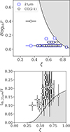 |
Fig. A.1. Accuracy criteria from Heisenberg. Top: Flux contrast (δlog10ℱ) adopted during the peak identification for 21 μm (blue squares) and CO(2-1) (black circles) observations, as a function of the average filling factor (ζ). Bottom: Measured tfb, 21 μm/τ as a function of ζ. The gray region indicates the parameter space where high filling factors biase our measurements of the tfb, 21 μm from Kruijssen et al. (2018). |
To validate the accuracy of our measurements, we verified that the requirements listed in Sect. 4.4 of Kruijssen et al. (2018) were fulfilled. The constrained parameters are measured with an accuracy of at least 30%, upon satisfaction of the following criteria :
-
(i) The duration of tCO and t21 μm (resp. tCO and tHα) should differ by less than one order of magnitude. This criterion is matched in all of our sample, both for CO versus Hα and CO versus 21 μm runs. We note that for one galaxy (NGC 3059), log10(t21 μm/tCO) ∼ 1.0.
-
(ii) The ratio λfb, 21/lap, min (resp. λfb, Hα/lap, min) should be below 1.5. For the Hα versus CO runs, this criterion is matched for all but two galaxies (NGC 4303 and NGC 4548) for which only upper limits are derived. We note the values we derive for λfb, Hα may slightly differ from K22 due to our updated mask. Hence, we report only an upper limit for NGC 4303 while a measurement was reported in K22. Conversely, we now provide measurements of tfb, Hα for NGC 1087, NGC 1385, and NGC 4540, while only an upper limit was derived in K22. For the runs with 21 μm, the combination of the high sensitivity of 21 μm maps tends to increase the number of detected peaks and decrease λ, while the aperture size is fixed by the worst resolution of all maps, i.e., the resolution of the ALMA/CO(2-1) maps. Hence, 31 out of 37 galaxies do not meet this criterion in the 21 μm versus CO runs. To enlarge our sample size, we slightly relax the recommended threshold and consider also as measurements galaxies for which λfb, 21/lap, min> 1.4, allowing us to include four additional galaxies visually associated with a clear decorrelation between 21 μm and CO (NGC 7496, NGC 0628, NGC 4731, and NGC 0685). The 25/37 galaxies with λfb, 21/lap, min ≤ 1.4, are flagged in our analysis (see Figure 4), as we can only derive an upper limit tfb, 21 μm, λfb, 21 μm, and tobs (see discussion in Section 3.4).
-
(iii) We verify that the number of identified peaks in both CO and Hα (respectively in both CO and 21 μm) emission maps is always above 35.
-
(iv) The CO-to-SFR flux ratios measured locally, focusing on CO (resp. Hα or 21 μm) peaks, is never below (resp. above) the galactic average. In the context of this analysis, we used a slightly more stringent criterion than the recommendation from Kruijssen et al. (2018) by imposing a Δmin > 0.05 (see Figure B.2), hence removing galaxies where no decorrelation was obtained between CO and 21 μm.
-
(v) The global star-formation history of the analyzed regions should not vary by more than 0.2 dex, during the last evolutionary cycle (τ = tgas + tstar - tfb), when averaged over a time period of tgas or tstar. A relatively stable SFR is expected in disk galaxies following a secular evolution, in particular when masking the central regions. For the subsample for which observations from the PHANGS-MUSE survey are available, we additionally ensure that this condition is verified based on the SFR histories measured in Pessa et al. (2023). (vi) Each region, independently undergoing evolution from gas to star, should be detectable in both tracers at some point in their life. This implies that sensitivity of the CO and 21 μm should be matched, allowing the faintest CO peak to evolve into H II regions that are bright enough to be detected in the 21 μm map. To verify this, we first compute the minimum mass of the young stellar population expected to form within the observed clouds, by multiplying the 5σ sensitivity of the CO maps (∼ 105M⊙; Leroy et al. 2021) by the integrated star-formation efficiencies reported in K22. This results in minimum young stellar population masses ranging from 800 M⊙ to 8000 M⊙, with a median value of ∼3600 M⊙. We then compare this value to the mass of a hypothetical young stellar population that emits photons at the 5σ sensitivity of the 21 μm map on the scale of star-forming regions (λ21 μm). We use the STARBURST99 model (Leitherer et al. 1999) to estimate Hα luminosity assuming instantaneous star formation, 5 Myr ago and a fully sampled initial mass function. The latter luminosity is converted to 21 μm emission using the conversion factor from Leroy et al. (2023b) to estimate the mass, resulting into a minimum young stellar population mass of ∼1500 M⊙. As a result, we find that the minimum young stellar population mass estimated for CO and 21 μm maps are in good agreement with each other within a factor of two (respectively three) for 13 galaxies (respectively 21) out of the 37 from our sample. For the rest of the sample, the greater sensitivity of the 21 μm observations compared to the CO ones biases the measured timescales associated with 21 μm (i.e., t21 μm, tfb, 21 μm, and tobscured toward larger values. We note that for most of the galaxies, the reported tfb, 21 μm and tobscured are already upper limits (see discussion Section 5.3). Hence, this bias does not affect our conclusions regarding the short duration of the embedded feedback phase (see Section 5.1).
-
(vii) When peaks are densely distributed, potentially overlapping with each other, the density contrast used for identifying peaks (δlog10ℱ) should be small enough to identify adjacent peaks. In the top panel of Figure A.1, we plot the density contrast used in each map of tracers as a function of the mean filling factor for gas and stellar peaks, defined as ζ = 1/(tCO + t21μm)×(tCO × ζCO + t21μm × ζ21μm), where ζCO= 2rCO/λfb, 21μm and ζ21μm= 2r21μm/λfb, 21μm with rCO (resp. r21μm) is the radii of the gas peaks (resp. SFR peaks). We confirm that our adopted values are small enough for all galaxies, compared to the upper limit identifying regions affected by blending from Kruijssen et al. (2018).
-
(viii) In order to check whether we sufficiently resolve independent regions, in the bottom panel of Figure A.1 we compare the analytical prescription of Kruijssen et al. (2018) with our measurements of tfb, 21 μm/τ, where τ is the total duration of the entire evolutionary cycle (τ = tCO + t21 μm - tfb, 21 μm). We confirm that the total duration of the evolutionary cycle is large enough for all galaxies compared to the upper limit identifying regions affected by blending from Kruijssen et al. (2018), except for NGC 5068 which lies slightly below the theoretical limit.
-
(ix) As shown in the lower panel of Figure A.1, we ensure that the conditions tfb, 21 μm/τ > 0.05 and tfb, 21 μm/τ < 0.95 are verified for all galaxies.
-
(x) Similarly to condition (v), the global SFR of the analyzed region should not vary more than 0.2 dex during the entire evolutionary lifecycle when averaged over tfb, 21 μm. This is satisfied using the same argument in (v) stated above.
-
(xi) After masking obviously crowed regions such as the galaxy center, visual inspection does not reveal abundant region blending. In conclusion, we find that our measurements are constrained with high accuracy for 12 out of 37 galaxies. For the remaining 25 galaxies, our analysis is mainly limited by the limited spatial resolution of the CO maps (criterion ii) and the difference in sensitivity (criterion v)), leading to the derivation of upper limits only for λfb, 21 μm, tfb, 21 μm, and tobscured.
Appendix B: Outputs from the Tuning-fork analysis
In this Section, we provide additional figures illustrating specific aspects of our analysis, which are mentioned throughout the text. In Figure B.1, we illustrate the filtering of the diffuse emission and peak identification (described in Section 3.2), that enable us to derive timescale measurements, based on the "tuning-fork" framework, as explained in Section 3.4. In Figure B.2, we show the 52 galaxies for which CO, Hα, and 21 μm maps are available and illustrate our selection criteria, described in Section 2.1, leading to a final sample of 37 galaxies. The resulting sample is presented in Table B.1, ordered by morphological type, along with the main input parameters used in our analysis. Table B.2 lists the values of physical quantities derived in our analysis, whose trends are discussed in Section 4.
For some of these parameters (tfb, 21 μm, tobscured, and λfb, 21 μm), robust measurements can only be derived in 12/37 galaxies in our sample, while only upper limits are obtained for the others. The correlations obtained for these parameters with various physical quantities are shown in Figure B.3. While these are based on a small number of objects, they are used to guide the discussion in Sections 5.2.1 and 5.2.2.
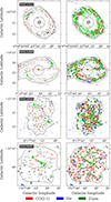 |
Fig. B.1. Composite image of four galaxies for which robust timescale measurements are derived. The galaxies are ordered following their Hubble morphological T-type from the LEDA database, from massive barred spiral galaxies to low-mass irregular galaxies. The left column shows the compact emission maps obtained after filtering the large scale component. On the right column, the superimposed crosses show the peaks of emission selected by CLUMPFIND (Williams et al. 1994) in each tracer. Isolated 21 μm peaks (green crosses) are identified in the interarm region of barred spiral galaxies, while most 21 μm peaks overlap with CO or Hα peaks in flocculent and irregular galaxies. The black masks show regions which are considered in our analysis, excluding galactic centers, bright peaks of emission, and outer regions where CO is undetected. |
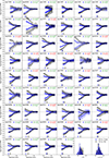 |
Fig. B.2. Deviation of the 21 μm-to-CO flux ratio (blue) and Hα-to-CO flux ratio (black) with respect to the galactic average as a function of aperture sizes for each galaxy. The arrows indicate the typical separation length, λ, at which the two tracers decorrelate. The amplitude of the decorrelation and the separation length are systematically smaller for CO versus 21 μm runs than for CO versus Hα runs, highlighting the greater overlap between CO and 21 μm. The legends indicate the criteria used to select our final sample: (1) a resolution R ≤ 180 pc (2) a clear decorrelation between CO and 21 μm with Δmin > 0.04 dex. |
Main input parameters used in the analysis for galaxies ordered by increasing Hubble morphological T-types.
Physical quantities associated with 21 μm describing the evolution timeline of molecular clouds.
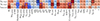 |
Fig. B.3. Spearman’s rank correlation coefficients measured between galaxy properties (columns) and our measurements (rows), adopting a methodology similar to the one described in Figure 6. The correlations derived for these quantities (λfb, 21 μm, tfb, 21 μm, and tobscured) are based only on the robust measurements are obtained for 12/37 galaxies. |
Appendix C: Updates compare to K22 analysis
One major update of our study is to account for the metallicity information available with the MUSE maps. In Figure C.1, we provide a comparison of the adopted ΣSFR-weighted metallicity average with other metallicity estimates that were used in previous studies. Finally, in Figure C.2 we provide a direct comparison of key parameters previously derived in K22, that we updated using new physical prescriptions and different masks. The modifications of the masked regions, as well as the new prescriptions adopted for metallicity and the CO-to-H2 conversion factors (see Section 2.3) involve variations of the predicted parameters compared to the previous analysis from K22. Nevertheless, the latter variations remain moderate for the predicted SFR, molecular gas masses (MH2) and the associated surface density (ΣSFR and ΣH2). In particular, while the predicted masses and SFR, which are sensitive to the covered area, tend to be smaller in the current study, we checked that the H2 and SFR surface densities do not vary more than a factor of two compared to the predictions from K22. Similarly, we also checked that all the quantities predicted by our method remain in good agreement with the values obtained in K22 within a factor of two to three. Most importantly, we show in Figure C.2 that the total cloud lifetime, used as the reference timescale in our study, remains in excellent agreement between both studies, varying by a factor of 1.5 at maximum.
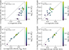 |
Fig. C.1. Comparison of the ΣSFR-weighted metallicity based on metallicity estimates obtained with MUSE data compared with (i) the integrated metallicity estimated from a direct conversion of the stellar mass based on the MZ relation from Sánchez et al. (2019) at the effective radius Reff; (ii) the metallicity estimates from Sánchez et al. (2019) at Reff, corrected assuming a fixed radial gradient within the galaxy (-0.1 dex/,Reff; Sánchez et al. 2014; iii) the metallicity estimated using the S-calibration (Pilyugin & Grebel 2016) at the median galactocentric radius of MUSE observations in Santoro et al. (2022); and (iv) metallicity estimates based on the maps from Williams et al. (2022). To ensure a meaningful comparison, all the estimates are averaged within the masks used in our analysis, excluding galactic centers. The color bar shows the stellar masses in log values. |
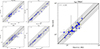 |
Fig. C.2. Comparison between the main physical quantities derived in K22 and the ones derived in this study when applying HEISENBERG to the same CO and Hα maps, within masks that correspond to the MIRI/21 μm observations, and adopting an updated CO-to-H2 conversion factor (see Section 3.1). Left: Comparison of the predicted molecular gas masses (upper left panel), H2 gas surface density (upper-right panel), SFR (bottom left panel), and SFR surface densities (bottom-right panel). Deviations remain moderate between both studies: most of our sample lie on the one-one relation while the few galaxies that deviate from previous measurements remain in good agreement within a factor of 2. Right: Comparison between the cloud lifetimes (tgas = tCO) derived in K22 and the ones derived in this study when applying HEISENBERG to the same CO and Hα maps, within masks that correspond to the MIRI/21 μm observations. Both measurements are in agreement within a factor of 1.5. |
Appendix D: Impact of masking extremely bright 21 μm peaks
The statistical method used in the current study provides flux-weighted measurements, averaged on the population of peaks detected in gas and stellar maps. In order to derive statistically meaningful averages, exceedingly bright peaks, identified as outliers in the peak luminosity function, need to be excluded. They represent a small fraction of the total number of detected peaks (median ∼ 1.4%, and < 3% in all galaxies), but contribute disproportionately to the emission (5-58%, with a median of 19%, see Table B.1).
In previous studies, the inclusion of such bright peaks has been found to significantly bias the measurements, leading to enlarged error bars on the derived quantities (e.g., Ward et al. 2022) or to overestimation of the timescale associated with the phase in which these bright peaks are captured (Chevance et al. 2020a). In other more favorable cases, the contribution from bright peaks may average out, and lead to measurements that remain compatible within the errors, regardless of the masking scheme considered (e.g., Kim et al. 2025). In Table D.1, we assess the effect of masking the brightest peaks in 21 μm for the subsample of galaxies for which robust timescales measurements could be derived, both including and excluding bright peaks.
For 8/26 galaxies, including bright peaks, most of the time captured in a phase emitting both CO and 21 μm simultaneously, flattens the tuning-fork upper branch, rendering robust measurements impossible. This effect is specific to the tracers considered in the current study, since the correlation between CO-and-21 μm is strong and already challenging to resolve (see Section 5.3). Based on the subsample where robust measurements could be derived with and without masking bright peaks, we find that including them tend to enlarge the uncertainties associated with λfb, 21μm, with no systematic increase or decrease. It also tends to moderately decrease all the timescales associated with 21 μm, although the results remain compatible within the errors.
Comparison of physical quantities associated with 21 μm described in Table B.2 with (default) and without (in parenthesis) masking bright peaks.
All Tables
Main input parameters used in the analysis for galaxies ordered by increasing Hubble morphological T-types.
Physical quantities associated with 21 μm describing the evolution timeline of molecular clouds.
Comparison of physical quantities associated with 21 μm described in Table B.2 with (default) and without (in parenthesis) masking bright peaks.
All Figures
|
Fig. 1. Composite image of the 37 galaxies drawn from the PHANGS surveys, ordered following their Hubble morphological T-type from the LEDA database, from massive spirals to low-mass irregular galaxies. All the maps have been convolved to the resolution of the ALMA/CO(2–1) maps, corresponding to the minimal aperture size reported in Table B.1. The white masks show regions that are excluded from our analysis (Hα and CO bright peaks identified in K22 as well as artifacts and diffraction spikes in any of the three tracers). The green circles show the brightest peaks in 21 μm, which are masked in our analysis, as described in Section 3.1. The number of masked peaks and corresponding surface brightness thresholds are reported in the Table B.1. |
| In the text | |
|
Fig. 2. Measured deviation of the gas-to-stellar flux ratio with respect to the galactic average as a function of the aperture sizes for each galaxy obtained by contrasting CO emission as a gas tracer respectively with Hα (black triangles) and 21 μm (blue circles) as an SFR tracer. The positive deviations correspond to measurements focusing on gas peaks (traced by CO), while the negative deviations were obtained by focusing on stellar peaks (traced respectively by Hα or 21 μm). For each data point, we also show the effective 1σ error, after the covariance between data points is taken into account. The horizontal plain line corresponding to a deviation of zero in log represents the galactic average. The dotted gray lines connecting the measurements correspond to a polynomial fit of the tuning-fork branches, following Kruijssen et al. (2018). The arrows indicate the typical separation length, λ, at which the two tracers decorrelate. The two last panels show the histograms of λ and inferred feedback timescales (tfb, defined in Section 3.3), derived for the whole sample using either Hα or 21 μm as a proxy for SFR, as well as the median and 1σ standard deviations associated with these distributions. |
| In the text | |
|
Fig. 3. Schematic evolutionary timeline of a star-forming region from the molecular cloud assembly until it becomes invisible in any of the three tracers we consider. In this study, we focus on the embedded feedback phase, during which stars are embedded within their host GMC. This phase is composed of an exposed phase, during which CO, 21 μm, and Hα emit simultaneously, and of an obscured phase, during which Hα emission is not detected. After the GMC dispersal, we measured an isolated phase of emission for both SFR tracers before they fade away. For most galaxies, 21 μm fades faster than Hα (upper arrow), but a few galaxies display a longer 21 μm emission (bottom arrow). |
| In the text | |
|
Fig. 4. Typical evolutionary timescales in our sample evolving from an inert CO-emitting phase to an embedded star-forming phase traced with 21 μm and eventually to an exposed star-forming phase traced with Hα emission. The feedback timescale tfb, 21 μm is an upper limit in 25 out of 37 galaxies, which are flagged with U. The upper and lower errorbars associated with each phase of the evolutionary cycle are shown as thin lines, with the same color. Galaxies are ordered by their Hubble morphological type. |
| In the text | |
|
Fig. 5. Feedback timescale measured based on 21 μm emission versus feedback timescale measured based on Hα. The color bar shows the Hubble morphological type from the HyperLEDA database (Paturel et al. 2003a,b; Makarov et al. 2014). The dotted line shows the 1:1 relation. The obscured feedback phase traced by 21 μm (tfb, 21 μm – tfb, Hα) is less than 4 Myr in all the galaxies from our sample, as shown by the plain black line, and less than 1 Myr for 28 out of 37 galaxies, as shown by the shaded area. We display the Spearman correlation coefficient as well as the log p-value of the data, excluding upper limits. |
| In the text | |
|
Fig. 6. Spearman’s rank correlation coefficients and associated p-values measured between galaxy properties (columns) and our measurements (rows). Statistically significant correlations according to the Holm-Bonferroni method (described in Section 4.2.2) are highlighted as black squares, and marginally significant correlations (log p-values < –2) are shown as blue squares. Our measurements are the total timescale of 21 μm emission (t21 μm), the ratio between timescales of SFR and gas(t21 μm/tCO), and the diffuse emission fractions of 21 μm (f |
| In the text | |
|
Fig. 7. Dependencies of the total duration of the 21 μm emitting phase (t21 μm). Left: Total duration of the 21 μm vs. CO-luminosity-weighted average velocity dispersion of GMCs. The color bar shows the CO luminosity-weighted average mass of GMCs. Galaxies with high surface density contrasts are identified with squares. We show in gray a linear regression fitted to the data and the gray-shaded area represents the 95% confidence interval on the regression, obtained with bootstrapping data. Right: Total duration of the 21 μm vs. the Hubble morphological type. The color bar shows the metallicity measurements for the galaxies observed with MUSE. |
| In the text | |
|
Fig. 8. Ratio of the total duration of the 21 μm emitting phase (t21 μm) over the total cloud lifetime (tCO) vs. H2 surface density estimated after filtering the diffuse CO emission. The color bar shows the total H I mass. |
| In the text | |
|
Fig. 9. Dependencies of the diffuse fraction of 21 μm emission (f21 μm, diffuse). Left: Diffuse fraction of 21 μm emission as a function of the global gas mass fraction. The color code shows the H2 gas mass fraction for each galaxy. Right: Diffuse fraction of 21 μm emission as a function of the kiloparsec-scale stellar surface density. The color bar shows the metallicity. |
| In the text | |
|
Fig. 10. Duration of the feedback time (tfb, 21 μm) as a function of the CO luminosity-weighted average velocity dispersion of molecular clouds. The color bar shows the CO luminosity-weighted average mass of GMCs. |
| In the text | |
|
Fig. 11. Dependencies of the duration of the obscured star-formation time (tobscured). Left: Duration of the obscured star-formation time as a function of the morphological type of galaxies from the HyperLEDA database (Paturel et al. 2003a,b; Makarov et al. 2014). The color bar shows the gas-phase metallicity measured with MUSE. Right: Duration of the obscured star-formation phase (bottom) as a function of gas-phase metallicity. The color bar shows the evolution of the SFR surface density. |
| In the text | |
|
Fig. A.1. Accuracy criteria from Heisenberg. Top: Flux contrast (δlog10ℱ) adopted during the peak identification for 21 μm (blue squares) and CO(2-1) (black circles) observations, as a function of the average filling factor (ζ). Bottom: Measured tfb, 21 μm/τ as a function of ζ. The gray region indicates the parameter space where high filling factors biase our measurements of the tfb, 21 μm from Kruijssen et al. (2018). |
| In the text | |
|
Fig. B.1. Composite image of four galaxies for which robust timescale measurements are derived. The galaxies are ordered following their Hubble morphological T-type from the LEDA database, from massive barred spiral galaxies to low-mass irregular galaxies. The left column shows the compact emission maps obtained after filtering the large scale component. On the right column, the superimposed crosses show the peaks of emission selected by CLUMPFIND (Williams et al. 1994) in each tracer. Isolated 21 μm peaks (green crosses) are identified in the interarm region of barred spiral galaxies, while most 21 μm peaks overlap with CO or Hα peaks in flocculent and irregular galaxies. The black masks show regions which are considered in our analysis, excluding galactic centers, bright peaks of emission, and outer regions where CO is undetected. |
| In the text | |
|
Fig. B.2. Deviation of the 21 μm-to-CO flux ratio (blue) and Hα-to-CO flux ratio (black) with respect to the galactic average as a function of aperture sizes for each galaxy. The arrows indicate the typical separation length, λ, at which the two tracers decorrelate. The amplitude of the decorrelation and the separation length are systematically smaller for CO versus 21 μm runs than for CO versus Hα runs, highlighting the greater overlap between CO and 21 μm. The legends indicate the criteria used to select our final sample: (1) a resolution R ≤ 180 pc (2) a clear decorrelation between CO and 21 μm with Δmin > 0.04 dex. |
| In the text | |
|
Fig. B.3. Spearman’s rank correlation coefficients measured between galaxy properties (columns) and our measurements (rows), adopting a methodology similar to the one described in Figure 6. The correlations derived for these quantities (λfb, 21 μm, tfb, 21 μm, and tobscured) are based only on the robust measurements are obtained for 12/37 galaxies. |
| In the text | |
|
Fig. C.1. Comparison of the ΣSFR-weighted metallicity based on metallicity estimates obtained with MUSE data compared with (i) the integrated metallicity estimated from a direct conversion of the stellar mass based on the MZ relation from Sánchez et al. (2019) at the effective radius Reff; (ii) the metallicity estimates from Sánchez et al. (2019) at Reff, corrected assuming a fixed radial gradient within the galaxy (-0.1 dex/,Reff; Sánchez et al. 2014; iii) the metallicity estimated using the S-calibration (Pilyugin & Grebel 2016) at the median galactocentric radius of MUSE observations in Santoro et al. (2022); and (iv) metallicity estimates based on the maps from Williams et al. (2022). To ensure a meaningful comparison, all the estimates are averaged within the masks used in our analysis, excluding galactic centers. The color bar shows the stellar masses in log values. |
| In the text | |
|
Fig. C.2. Comparison between the main physical quantities derived in K22 and the ones derived in this study when applying HEISENBERG to the same CO and Hα maps, within masks that correspond to the MIRI/21 μm observations, and adopting an updated CO-to-H2 conversion factor (see Section 3.1). Left: Comparison of the predicted molecular gas masses (upper left panel), H2 gas surface density (upper-right panel), SFR (bottom left panel), and SFR surface densities (bottom-right panel). Deviations remain moderate between both studies: most of our sample lie on the one-one relation while the few galaxies that deviate from previous measurements remain in good agreement within a factor of 2. Right: Comparison between the cloud lifetimes (tgas = tCO) derived in K22 and the ones derived in this study when applying HEISENBERG to the same CO and Hα maps, within masks that correspond to the MIRI/21 μm observations. Both measurements are in agreement within a factor of 1.5. |
| In the text | |
Current usage metrics show cumulative count of Article Views (full-text article views including HTML views, PDF and ePub downloads, according to the available data) and Abstracts Views on Vision4Press platform.
Data correspond to usage on the plateform after 2015. The current usage metrics is available 48-96 hours after online publication and is updated daily on week days.
Initial download of the metrics may take a while.