| Issue |
A&A
Volume 706, February 2026
|
|
|---|---|---|
| Article Number | A368 | |
| Number of page(s) | 22 | |
| Section | Extragalactic astronomy | |
| DOI | https://doi.org/10.1051/0004-6361/202556455 | |
| Published online | 24 February 2026 | |
The Next Generation Fornax Survey (NGFS)
VIII. A support vector machine approach to disentangling globular clusters
1
Instituto de Estudios Astrofísicos, Facultad de Ingeniería y Ciencias, Universidad Diego Portales Av. Ejército Libertador 441 Santiago, Chile
2
Instituto de Astrofísica, Pontificia Universidad Católica de Chile Av. Vicuña Mackenna 4860 Santiago 7820436, Chile
3
Instituto de Astrofísica, Universidad Andres Bello Fernandez Concha 700 Las Condes Santiago, Chile
4
Vicerrectoría de Investigación y Postgrado, Universidad de La Serena La Serena 1700000, Chile
5
University of Calgary 2500 University Drive NW Calgary Alberta T2N 1N4, Canada
6
International Gemini Observatory/NSF NOIRLab Casilla 603 La Serena, Chile
★ Corresponding author: This email address is being protected from spambots. You need JavaScript enabled to view it.
Received:
17
July
2025
Accepted:
17
December
2025
Abstract
Context. Wide-field, multiband surveys are capable of detecting millions of unresolved sources in nearby galaxy clusters; however, separating globular clusters (GCs) from foreground stars and background galaxies remains challenging. Scalable and automated classification methods are therefore essential to transform forthcoming data from facilities such as the Vera C. Rubin Observatory Legacy Survey of Space and Time (LSST), Euclid, and the Nancy Grace Roman Space Telescope into robust constraints on galaxy assembly.
Aims. We present a supervised machine-learning method to separate GCs, stars, and galaxies using their distribution in color-color space. The primary objective is to recover a clean and reliable GC sample optimized for next-generation survey volumes.
Methods. We analyzed the central 3 deg2 of the Next Generation Fornax Survey (NGFS), which images the Fornax cluster in u′g′i′ (BLANCO/DECam) and JKs (VISTA/VIRCAM). We trained a support vector machine (SVM; svm.SVC implemented in scikit-learn) using spectroscopically confirmed sources. The initial model employed 15 features, including all color combinations from u′g′i′JKs and basic morphological parameters (e.g., FWHM and ellipticity).
Results. Color combinations linking near-ultraviolet (NUV) and optical to near-infrared (NIR) wavelengths, particularly (u′−g′) versus (g′−Ks), provide the strongest discrimination among object classes. The full 15-feature model achieves an accuracy of 97.3%. A reduced seven-feature model, built from the most informative and least correlated features, attains a 96.6% level of accuracy with a misclassification rate of 10.4%, offering a more efficient and robust solution. Excluding the u′ or NIR bands significantly degrades performance. Tests using LSST-like filters, constructed from NGFS u′g′i′ and Dark Energy Survey r′z′Y data, show that the u′ and Y bands are essential, although models lacking NIR coverage remain suboptimal.
Conclusions. Broad spectral energy distribution coverage combined with simple morphological parameters enables an accurate and scalable classification of unresolved sources. The inclusion of NIR data substantially improves GC identification and the joint exploitation of LSST with Euclid and Roman observations will further enhance machine-learning approaches in large extragalactic surveys.
Key words: methods: data analysis / methods: statistical / techniques: photometric / galaxies: clusters: general / galaxies: general / galaxies: star clusters: general
© The Authors 2026
 Open Access article, published by EDP Sciences, under the terms of the Creative Commons Attribution License (https://creativecommons.org/licenses/by/4.0), which permits unrestricted use, distribution, and reproduction in any medium, provided the original work is properly cited.
This article is published in open access under the Subscribe to Open model. This email address is being protected from spambots. You need JavaScript enabled to view it. to support open access publication.
1. Introduction
Globular clusters (GCs) occupy a singular niche in astrophysics: they are among the oldest and simplest stellar systems in the Universe (e.g., Vandenberg et al. 1996; Willman & Strader 2012). They encode the earliest star formation and assembly events of their host galaxies (e.g., Ashman & Zepf 1992; Brodie & Strader 2006; Chen et al. 2025). Systematic studies over the past decades have shown that essentially every galaxy more massive than ∼ 108 M⊙ (stellar mass) hosts a GC system whose chemical compositions, kinematics, sizes, and spatial distribution mirror the host’s evolution and merger history (e.g., Forbes et al. 1997; Puzia et al. 2005, 2006; Peng et al. 2006; Chies-Santos et al. 2022). Because GCs’ colors, age-metallicity scaling relations, and specific frequencies are tightly correlated with the host halo mass (e.g., Georgiev et al. 2010; Harris et al. 2013; Forbes et al. 2018), they have become widely used tracers of dark matter assembly on galactic and cluster scales (Cooper et al. 2025; Chen et al. 2025). In dense environments such as galaxy clusters, GCs also contribute to understanding environmental effects on galaxy evolution (e.g., Smith et al. 2015; Lim et al. 2024) and intracluster light (ICL) formation (e.g., Peng et al. 2011; Alamo-Martínez et al. 2013; Madrid et al. 2018; Kluge et al. 2025).
Accurate identification of GCs serves as an additional means to comprehend the formation and evolution of galaxies. Deep imaging from state-of-the-art ground-based and space-based observatories has significantly improved the photometric characterization of GCs. Despite the depth and quality of modern imaging, separating GCs from stars and background galaxies remains challenging due to overlapping photometric and morphological properties (e.g., Puzia et al. 2014). Traditional selection criteria based on color cuts or structural parameters fail to disentangle these various stellar systems properly, producing contamination fractions of 30–70% in purely optical photometric samples (e.g., Powalka et al. 2016), unless sample statistics overwhelmingly point in favor of GCs; for instance, in brightest cluster galaxies (Harris & Reina-Campos 2024). Decontamination becomes particularly challenging in the central regions of galaxy clusters or in the vicinity of their massive and regular galaxies, where their light profile affects the detection and photometry of stars (foreground), GCs (cluster), and galaxies (background), which can significantly reduce the GC catalog purity and thereby complicate the interpretation of GC samples (e.g., Durrell et al. 2014; Lim et al. 2025).
Muñoz et al. (2014) showed that by incorporating a broader wavelength baseline, particularly including the u′ and Ks band, the separation between GCs and other sources becomes clearer, as these bands enhance the contrast in the SED properties between the stellar systems. The scientific return from extragalactic GC studies has grown in lock-step with advances in wide-field, optical/NIR imaging (e.g., Muñoz et al. 2014; Taylor et al. 2017). Surveys such as the Next Generation Virgo Survey (NGVS, Ferrarese et al. 2012), the Next Generation Fornax Survey (Muñoz et al. 2015; Eigenthaler et al. 2018; Ordenes-Briceño et al. 2018), PHANGS–HST (e.g., Maschmann et al. 2024), and, more recently, deep Euclid pilot programs now detect thousands of GC candidates per pointing (Saifollahi et al. 2025), probing out to larger galactocentric radii and lower surface-brightness regimes than ever before. Spectroscopic studies are infeasible for the millions of candidates predicted by modern cosmological simulations (e.g., E–MOSAICS, see Pfeffer et al. 2018) and for the 350 000 estimated GCs in the Euclid footprint (Euclid Collaboration: Voggel et al. 2025b) and ≳4 × 10⁶ GCs forecast to be visible in the Vera C. Rubin – LSST imaging (Ivezić et al. 2019; Usher et al. 2023).
These data volumes demand scalable, fully automated classification pipelines. Machine-learning (ML) methods have already demonstrated superior performance over traditional approaches in many domains of astronomy (e.g., Angora et al. 2019; Saifollahi et al. 2021; Barbisan et al. 2022; Chies-Santos et al. 2022; Ting et al. 2025). Among “classical” algorithms, the support vector machine (SVM) remains appealing because it yields interpretable decision boundaries (Cortes & Vapnik 1995; Platt 1999a; Crammer & Singer 2002), is robust against the “curse of dimensionality” (e.g., Joachims 1998; Guyon et al. 2002), and can be tuned efficiently with modest training sets (Chapelle et al. 2002). SVMs have been applied successfully to classifications of galaxy morphology (e.g., Huertas-Company et al. 2008; Vavilova et al. 2021), stellar objects and transients (Li et al. 2025), and spectral lines (Shi et al. 2015), as well as to the identification of active galactic nuclei (AGNs), galaxies, and stars, with ≲5% cross-contamination (Małek et al. 2013; Cenarro et al. 2019; Wang et al. 2022).
In this work, we advance these efforts by developing a supervised SVM pipeline using the NGFS’s ultra-deep, broad spectral baseline imaging, spanning u′g′i′JKs and morphological parameters, to classify point-like sources in GC, star, and galaxy categories. We used Python with its sklearn library1 (Pedregosa et al. 2011). Our SVM classifier is immediately applicable to forthcoming data releases from Vera C. Rubin-LSST, Euclid, and Roman Space Telescope, where rapid and reliable GC identification will be critical for studies of galaxy assembly, stellar population gradients, and GC formation efficiencies across diverse environments.
The structure of this paper is organized as follows. Section 2 summarizes the NGFS data and catalog construction. Deep color-color diagrams (cc-diagrams) are presented in Section 3. Section 4 describes the SVM methodology, feature selection and hyper-parameter optimization. Results for the full and reduced filter sets are given in Section 5. In Section 6, we assess expected performance for LSST-like photometry. Section 7 summarizes our conclusions and outlines future applications.
2. Data
The present study makes use of data from the NGFS, a deep, multiwavelength survey of the Fornax galaxy cluster that extends out to a projected radius of 1.4 Mpc, which encloses a total cluster mass of 7 × 10¹³ M⊙ (Drinkwater et al. 2001). Optical photometry was obtained using the Blanco 4-meter telescope equipped with the Dark Energy Camera (DECam; Flaugher et al. 2015), covering a total of 19 tiles (≃57 deg2) complete in three bands: u′, g′, and i′, where one DECam tile has a field of view (FoV) of 2.2 deg. Additionally, NGFS includes a NIR component observed with the VISTA telescope using the VISTA InfraRed CAMera (VIRCam; Sutherland et al. 2015, now decommissioned), providing J and Ks band data over 12 central tiles (≃20 deg2), with a VIRCam tile FoV of 1.6 deg. The specific preparation of the NGFS optical dataset in u′g′i′ for the 19 tiles will be presented in a dedicated paper (NGFS et al., in prep.), which includes a detailed description of data reduction, photometric calibration, completeness tests, and final photometry.
The analysis focuses on the central region of the Fornax cluster, hereafter referred to as NGFS-T1. This region is composed of T1 DECam (u′g′i′) and T1 and T2 VIRCam (JKs) observations. The pixel scale is 0.263″ and 0.339″ for DECam and VIRCam, respectively. The data reduction pipeline for NGFS-T1 is described in the PhD thesis of Ordenes Briceño (2018). Here, we include a brief description of the data reduction and photometric calibration in Appendix A. The VIRCam central tile is composed of two tiles; however, the final science image consists of a single stacked image per band, covering a FoV of 1.6 deg × 2.2 deg, highlighted in Figure 1 as a superposed red rectangle.
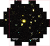 |
Fig. 1. RGB composite image of NGFS Tile 1, constructed using DECam filters (i′ in red, g′ in green, and u′ in blue). The field of view corresponds to a single DECam tile, with a radius of 1.1° ≈370 kpc at the distance of the Fornax cluster (D = 19.3 Mpc; Anand et al. 2024). The NIR imaging FoV is shown with an unfilled red rectangle (see Sect. 2 for details). The names of the main galaxies are indicated, with the cD galaxy NGC 1399 located near the image center. Angular and physical scales are shown: the white line in the bottom-right represents 0.25° and the line in the bottom-left corresponds to 100 kpc. |
We have revised the photometric calibration of the complete survey (see Fig. A.1). This includes the five science images of NGFS-T1, spanning from the near-ultraviolet (NUV) to the near-infrared (NIR): u′g′i′JKs. For instance, GC candidates at the Fornax distance (D = 19.3 Mpc; Anand et al. 2024) appear as unresolved sources owing to the spatial resolution limitations of the DECam (1 pix = 24.46 pc) and VIRCam (1 pix = 31.62 pc) instruments.
The central region of the Fornax cluster has a high galaxy density and, thus, the extended surface-brightness profiles of these galaxies hinder source detection, with many faint GCs being obscured by their diffuse light. To mitigate this effect, we implemented a point-source detection image following the procedure described in Appendix A.2, with Fig. A.2 illustrating the result. Photometry was performed with Source Extractor (SExtractorBertin & Arnouts 1996), using the detection catalog as a prior to obtain the cleanest possible photometry for sources projected behind the galaxies.
We constructed a point spread function (PSF) model with PSF Extractor (PSFexBertin 2011), which accounts for PSF variations across the detectors. The final photometric catalogs provide magnitudes (PSF, APER, AUTO) in the optical passbands in the AB system. The NIR magnitudes were transformed from the Vega to the AB system using Ks(mAB − mVega) = 1.85 mag and J(mAB − mVega) = 0.91 mag (Blanton & Roweis 2007).
Magnitudes were corrected for Galactic extinction toward the Fornax cluster, adopting Au′ = 0.054, Ag′ = 0.041, Ai′ = 0.020, AJ = 0.009, and AKs = 0.004 (Fitzpatrick 1999; Schlegel et al. 1998; Schlafly & Finkbeiner 2011). The extinction corrected photometry is shown in color-magnitude diagrams (CMDs) and cc–diagrams, using the subscript “0” for both magnitudes and colors.
The primary master catalog for NGFS-T1 consists of PSF photometry with complete SED cross-matching in the u′, g′, i′, J, and Ks bands, containing a total of 65 581 sources. To ensure a high photometric quality, we used the SExtractor output parameter FLAGS to select sources with no extraction issues (FLAGS = 0). This criterion guards against the presence of bad pixels, close neighbors, and deblended or saturated sources (i.e., FLAGS > 0). After applying this selection across all filters, the final sample comprised 62 416 sources.
For the purposes of this work, a completeness analysis was not required, but the effective depth of the data was instead defined by the limiting magnitudes of the u′ and Ks bands, which are the shallowest in the NGFS observations. The faintest objects in the five-filter matched catalog have magnitudes of u′ = 28.05 (mean u′ = 23.96), g′ = 26.46 (mean g′ = 23.17), i′ = 25.37 (mean i′ = 21.92), J = 24.90 (mean J = 21.23), and Ks = 23.63 (mean Ks = 21.23), all in the AB magnitude system. A completeness analysis will be presented in a follow-up paper.
For the subsequent analysis, we constructed the colors using PSF magnitudes in all filters. We adopted colors rather than magnitudes because the latter are distance dependent, whereas colors are independent of distance and therefore more robust and appropriate for relative comparisons and source classification. We used the following parameters from the master catalog: coordinates, colors, full width at half maximum (FWHM), flux radius (FR), spread model (SM), ellipticity (e), and the concentration index parameter (Cλ).
The SM parameter is an output of the photometry obtained with SExtractor when using a PSF model created with PSFex. It compares the source light profile with the PSF model, thereby indicating whether a source is more consistent with a point source or an extended source. Other structural parameters in the catalog include the FR, defined as the radius (in pixels) enclosing 50% of the total flux of the source; the FWHM, defined as the width of the source brightness profile at half its maximum intensity; and the ellipticity, defined as e = 1 − b/a, where a and b are the semimajor and semiminor axes, respectively.
An additional parameter is the concentration index Cλ, estimated as Cλ = MAG_APER(2 pix)−MAG_APER(8 pix) (Powalka et al. 2016). Small values of Cλ indicate that the light is predominantly concentrated in the PSF core (i.e., a compact source such as a star), whereas larger values correspond to more extended light profiles (e.g., galaxies).
These parameters are measured using i′-band photometry, which provides the best image quality among the u′, g′, J, and Ks bands in terms of seeing and depth. The average FWHM for point sources in the u′, g′, and i′ bands is 6.4 pixels (1.68″), 4.2 pixels (1.08″), and 3.6 pixels (0.95″), respectively.
NGFS-T1 covers a radius of r = 1.1° ≃370 kpc in the DECam FoV and r = 0.8° ≃268 kpc in the VIRCam FoV, both centered on the giant elliptical, or central dominant (cD), galaxy NGC 1399 (see Fig. 1). This tile provides an ideal test case for the ML method because of the high density of galaxies and GCs, which makes the separation of different stellar systems particularly challenging.
3. Deep color-color diagrams
From the NGFS-T1 master catalog with PSF photometry in the u′, g′, i′, J, and Ks bands, we constructed ten cc–diagrams using different filter combinations, always ordered from blue to red wavelengths (see Fig. 2). Each panel shows the NGFS-T1 sources as gray dots, while spectroscopically confirmed GCs, stars, and galaxies are shown in blue, gold, and purple, respectively. Further details about these confirmed samples are provided in Sect. 4.2.
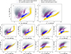 |
Fig. 2. Color-color diagrams for all sources with multiwavelength photometry in the core region of the Fornax cluster, shown as gray dots. Spectroscopically confirmed samples of GCs (blue), stars (gold), and galaxies (purple) are highlighted and used as labeled samples for the svm.SVC model (see Sect. 4.2). Note: the different panels show the same source sample, for which photometric information was obtained from the master catalog cross-matched across the u′g′i′JKs filters. |
In Fig. 2 (top-left: panel A), we give the (u′−g′) versus (g′−Ks) diagram, hereafter referred to as u′g′Ks. This naming convention is also applied to the other filter combinations. These cc–diagrams demonstrate the diagnostic utility of combining NUV and NIR filters to distinguish between different stellar populations and object types in deep, wide-field imaging.
In diagrams such as u′g′Ks (panel A), u′i′Ks (panel B), and u′JKs (panel F), four main populations can be identified: background galaxies at various redshifts, passive early-type galaxies, Fornax cluster GCs, and foreground Milky Way stars (see also Muñoz et al. 2014). In contrast, these populations are less clearly separated in diagrams that lack the u′ band or where the filter wavelengths are more closely spaced, for example, in the third row, from g′i′J to the rightmost panels (panels G–J).
In the u′g′i′ diagram (panel C), only three distinct sequences are clearly visible, with the GC sequence overlapping the bluer region of the foreground stellar sequence. Nevertheless, this diagram retains diagnostic power for distinguishing between unresolved point sources and more extended objects (see also Fig. 3).
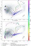 |
Fig. 3. Color–color diagrams u′g′Ks (top panel) and u′g′i′ (bottom panel) including PEGASE.2 population-synthesis models (Fioc & Rocca-Volmerange 1997). The layout is the same as in Fig. 2. In the top-panel diagram, the thin blue lines represent sequences of old single-age stellar populations at redshift zero; the corresponding metallicity range is indicated in the legend. The large colored symbols show the redshift evolution of observed colors for four galaxies formed at z = 3, each characterized by a different star-formation history: burst plus low star-formation rate (squares), constant star-formation rate (stars), exponentially declining star-formation rate (triangles), and burst followed by passive evolution (elliptical; circles). |
Choosing appropriate color combinations, for example, the u′i′Ks diagram (Muñoz et al. 2014), maximizes the separation between GCs and stars and galaxies in the color-color space. However, when a single color–color plane is used to select a sample, a significant level of contamination may still be present.
For instance, González-Lópezlira et al. (2017) used the u′i′Ks diagram to select GC candidates around the spiral galaxy NGC 4258, identifying 39 candidates. After applying completeness corrections, extrapolating the GC luminosity function, correcting for spatial coverage, and assuming a contamination fraction of 5%, they derived a total population of  (random and systematic uncertainties, respectively). In a spectroscopic follow-up of 23 GC candidates (González-Lópezlira et al. 2019), 70% were confirmed as GCs, while the remaining 30% were contaminants. This led to a revised estimate of NGC = 105 ± 26, including random uncertainties only, still implying a substantial contamination fraction.
4. Method: Support vector machine
Figure 2 illustrates the complexity of disentangling different stellar systems in deep cc–diagrams. Although NUV-optical-NIR filter combinations are very helpful, significant source overlap remains in some regions of parameter space, making it difficult to isolate a single population with low contamination. Therefore, our classification strategy must be capable of exploiting the available inputs to identify an optimal solution for this dataset, enabling the separation of three astrophysical sources: GCs, foreground stars, and background galaxies.
4.1. Support Vector Machine algorithm
SVMs are machine-learning methods primarily used for classification, but they can also be applied to detect outliers and perform regression (predicting values). In this work, we use a support vector classification algorithm implemented as sklearn.svm.SVC in the scikit-learn package (Pedregosa et al. 2011), hereafter referred to as svm.SVC. In simple terms, svm.SVC works by finding the optimal decision boundary, known as a hyperplane, that separates different groups (classes) of data points based on their characteristics (features). The algorithm goal is to find the boundary that maximizes the margin (i.e., the largest possible separation between classes). Only the data points closest to this boundary, known as support vectors, are used to define the hyperplane. These support vectors are critical to the model, as they determine the position and orientation of the hyperplane and ultimately influence how new data points are classified (Platt 1999a,b; Crammer & Singer 2002; Pedregosa et al. 2011).
In cases where the classes are not perfectly separable owing to overlapping distributions or the presence of noise in the data, the SVM employs the soft-margin technique (Crammer & Singer 2002). This approach introduces a degree of tolerance for misclassified samples, while still aiming to maximize the margin between classes. In this way, the model balances between the complexity and classification accuracy, thereby enhancing the robustness to outliers.
Thus, the SVM benefits from projecting the input data into a higher-dimensional space, where the classes may become linearly separable through the use of kernel functions. This kernel-based mapping allows the SVM to effectively capture complex class boundaries. The mathematical formulations of the kernel functions commonly used in SVMs are:
 (1)
(1)
 (2)
(2)
 (3)
(3)
 (4)
(4)
Here, x and x′ are input vectors, r is a constant, and d is the degree of the polynomial kernel. The parameter γ controls the influence of individual training examples: a small γ implies a larger region of influence (i.e., a smoother decision boundary), whereas a large γ implies a narrower region of influence, which can lead to overfitting by capturing noise in the data.
Therefore, C acts as a penalty parameter for misclassified points. It modifies the optimization objective by adding a penalty term for margin violations. For weighting a specific group or class, we use the class_weight parameter. Specifically, we use class_weight = ‘balanced’, for adjusting the penalty applied to each class based on their frequency in the training set.
The svm.SVC classifier is strongly influenced by the regularization parameter C, although this parameter does not appear explicitly in the kernel equations. It controls the trade-off between achieving a low training error and maintaining a large margin, which is fundamental to the soft-margin SVM formulation. For example, a small value of C favors a wider-margin hyperplane, even if this results in more misclassifications. Conversely, a larger value of C forces the model to fit the training data more strictly in order to minimize training errors, potentially leading to an overfitting, particularly in the presence of noise or outliers. Therefore, C acts as a penalty parameter for misclassified points by modifying the optimization objective through the addition of a penalty term for margin violations. To weight specific classes, we used the class_weight parameter. In particular, we adopted class_weight = balanced, which adjusts the penalty applied to each class according to its frequency in the training set.
4.2. Classes, training, and test dataset
For the training and testing of the SVM models, we required a confirmed sample for each class. We refer to this as the labeled sample, consisting of spectroscopically confirmed sources. Below, we describe the origin of the labeled sample.
To compile this sample, we used two reference studies to identify all objects with confirmed radial velocities within the area covered by NGFS-T1. The first is Chaturvedi et al. (2022), which focuses on the GC population within 0.7 Mpc of NGC 1399. The second is Maddox et al. (2019), which provides a catalog of sources in the Fornax region out to 1.4 Mpc, encompassing the main Fornax cluster and the Fornax A subgroup, and includes stars, GCs, and both cluster and background galaxies. These studies compile spectroscopic data from the following individual catalogs: Ferguson (1989), Kissler-Patig et al. (1999), Hilker et al. (1999, 2007), Drinkwater et al. (2000, 2001), Mieske et al. (2002, 2004, 2008), Bergond et al. (2007), Gregg et al. (2009), Schuberth et al. (2010), Chilingarian et al. (2011), Pota et al. (2018), Fahrion et al. (2020).
We did not apply any parameter cuts to the final catalog of RV-confirmed objects. However, when cross-matching the photometric and spectroscopic catalogs, some confusion could arise owing to projection effects in the images. For example, sources with nearby companions or extended morphologies may yield less reliable PSF photometry. This confusion can manifest in the cc–diagrams as objects labeled as GCs appearing outside the typical GC locus and instead falling within the galaxy region.
When applying this methodology to large survey datasets, even in the presence of contaminant inputs in the SVM model, the analysis must remain as automated as possible, with minimal manual intervention. Taking this into account, we divided the objects into three main classes, as follows:
-
Class 1: Globular clusters. This class includes 1209 objects with RV confirmation as GCs from the catalogs described above. Within a projected radius of 0.7 Mpc, Chaturvedi et al. (2022) estimated a total GC population of approximately 2300 sources. However, the cross-match between the complete RV-confirmed GC sample and the NGFS-T1 catalog, which covers a smaller area (< 0.34 Mpc), yielded roughly half of this population.
-
Class 2: Foreground stars. The compilation by Maddox et al. (2019) reports 9483 stars with RV confirmation within the Fornax cluster region (< 1.4 Mpc). In the same area, the Gaia mission EDR3 distance catalog (Gaia Collaboration 2021) detected and characterized a total of 9595 stars. Cross-matching these samples with the NGFS-T1 master catalog resulted in a final labeled sample of 2151 stars.
-
Class 3: Galaxies. The RV-confirmed galaxy sample from the Maddox et al. (2019) compilation contains a total of 6722 galaxies, including both Fornax cluster members and predominantly background galaxies. After cross-matching with the NGFS-T1 catalog, the final labeled sample consisted of 1587 galaxies within the NGFS-T1 area. We chose to retain objects classified as ultra-compact dwarf galaxies (UCDs) within class 1 (GCs). Although we acknowledge the uncertain nature of these objects, distinguishing between genuinely massive GCs and stripped galaxy nuclei is beyond the scope of this work. Using only a magnitude criterion of i < 20 (Mieske et al. 2002), the approximate number of UCDs in the RV catalog is 100–120 sources. In our svm.SVC model, we do not distinguish between galaxy subtypes (e.g., QSOs), as this is a complex task given the limited spatial coverage (∼0.34 Mpc; see Fig. 3). Maddox et al. (2019) reported 264 objects classified as QSOs out of a total of 6334 background galaxies, corresponding to 4.2% within a 1.4 Mpc radius. Therefore, for the NGFS-T1 field of view (0.34 Mpc), the expected QSO fraction is below 1%. A similar estimate was reported by Cristiani et al. (2001).
Figure 3 shows the cc–diagrams (u′g′Ks and u′g′i′), using the same layout as panels A and C in Fig. 2, respectively. In the u′g′Ks diagram (top panel), the blue lines represent old single-age stellar population (SSP) models at redshift zero, which closely trace the locus of the Fornax cluster GC population (blue circles, corresponding to the 1209 RV-confirmed GCs in class 1). In addition, we plot the redshift evolution of four prototypical galaxy SEDs formed at z = 3, each characterized by a different star-formation history (SFH). These tracks were computed using the DECam u′g′i′ and VIRCam JKs filter throughput curves to obtain observed colors with the population-synthesis code PEGASE.2 (Fioc & Rocca-Volmerange 1997). The four galaxy models correspond to: (a) a galaxy that formed most of its stars at high redshift and subsequently maintained a low, constant star-formation rate (squares); (b) a galaxy with a constant star-formation rate (stars); (c) a galaxy with an exponentially declining star-formation rate (triangles); and (d) a “red and dead” galaxy that formed all its stars at z = 3 and evolved passively thereafter (circles). This figure highlights the diversity and complexity of galaxy SFH that populate deep cc–diagrams.
With the three confirmed training samples established, we split the complete NGFS-T1 catalog into two subsets: a labeled sample, used for training and testing, and an unlabeled sample, used for classification. The labeled sample includes objects with known classifications: GCs, foreground stars, and background galaxies, whereas the unlabeled sample consists of sources with no prior classification.
The training and testing workflow consists of the following essential steps:
-
Split the labeled sample randomly into training and testing subsets using train_test_split. To define the fraction of the total sample used for training and testing, we explored several combinations: 80%/20%, 70%/30%, 60%/40%, and 50%/50%. The results are presented in Section 4.4.
-
Undersample the training set using RandomUnderSampler to address class imbalance, specifically the overrepresentation of galaxies relative to stars and GCs. This step reduces the sample size of the majority class, helping the model learn more effective decision boundaries across all classes.
-
Scale the resampled training set using StandardScaler. Since svm.SVC relies on distance-based metrics, feature scaling is particularly important when using the RBF kernel. Each feature is rescaled to have zero mean and unit variance, using the mean (μ) and standard deviation (σ) computed from the training set. This ensures that all features contribute on a comparable scale to the SVM optimization and prevents features with larger numerical ranges from dominating the model.
-
Scale the test set using the same scaler fitted to the training data, ensuring consistency between the training and test sets.
-
Train the classifier using svm.SVC, setting class_weight = ‘balanced’ to account for any remaining class imbalance and evaluate its performance on the test set.
-
Finally, apply the trained model to classify the remaining unlabeled sources in the catalog.
4.3. Searching for the best kernel function and parameters
In Section 4.1, we describe the different kernels available and the parameters in Eqs. (1)–(4), which can be adjusted to influence how the svm.SVC model learns. The efficiency of the model depends on the choice of kernel and on the structure of the data, in particular on whether the feature space is approximately linear or nonlinear.
To identify the most suitable combination of kernel and hyperparameters for our dataset, we use GridSearchCV from scikit-learn.model_selection, which performs an exhaustive search over a specified grid of parameters by training and validating the model for all possible combinations of the given hyperparameter values. For each combination, the model performance is evaluated using cross-validation, and the configuration that yields the best score is selected. We also fix the random state to a constant value (RS = 42) to ensure reproducibility of the results. We adopt the following param_grid:
-
RBF kernel: γ= [‘scale’, 1, 0.1, 0.01, 0.001, 0.0001];
-
polynomial kernel: degree= [2, 3, 4, 5];
-
sigmoid kernel: γ= [‘scale’, 1, 0.1, 0.01, 0.001, 0.0001].
For each of these kernels, we explored a regularization parameter grid of C = [0.1, 1, 10, 100, 1000]. This search was performed after steps (i)–(iv), described in the previous section, using the scaled training sample. The optimal parameters are C = 10 and γ = 0.1 or γ= ‘scale’, as reported in Sect. 5 and indicated in the titles of the corresponding figures. Therefore, the GridSearchCV procedure optimizes the SVM hyperparameters (C, γ, and kernel type) by systematically exploring the parameter space through cross-validation. This process ensures that the selected kernel and hyperparameters correspond to the best-performing configuration for our dataset.
4.4. Implementation of svm.SVC model
Feature selection in SVM is a critical step in optimizing model performance. Figure 2 illustrates how different color combinations contribute to separating the various populations present in the field. For the five filters used (u′g′i′JKs), we construct ten color indices, considering only those defined as magnitude differences between a bluer and a redder filter.
In addition to colors, we incorporate the morphological parameters of the sources (hereafter morpho-parameters), such as size, shape, and light profile, to improve the classification. As described in Sect. 2, the parameters used are: SPREAD MODEL, FLUX RADIUS, FWHM, ellipticity, and concentration index. By combining the colors and morpho-parameters, we provided a total of 15 features (15F) as input to the svm.SVC model (see Table 1).
Description for the 15 features (15F) provided for the model.
To obtain the best validation performance of the model, we used GridSearchCV, which cross-validates the hyperparameters (see Sect. 4.3) using the training portion of the data. During this process, the training set was further divided into multiple cross-validation folds. For each candidate kernel and hyperparameter combination, the model was trained on a subset of the folds and validated on the remaining ones, iteratively. The combination yielding the best validation performance was then selected and the model with these optimal parameters was retrained on the full training set and evaluated on the test set.
Another aspect affecting the validation performance is the random split of the labeled sample into training and testing subsets using train_test_split. We explore several train+test combinations: 80%/20%, 70%/30%, 60%/40%, and 50%/50%. The best performance is obtained for a split of 70% training and 30% testing, as shown in Figs. 4 and 6. For reference, the results for the other splits are presented in Appendix C.1.
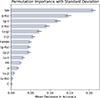 |
Fig. 4. Best-performing model accuracy and classification scores for a 70%/30% train/test split using an RBF kernel with C = 10 and γ = 0.1. The permutation feature importance for the 15 input features used by the svm.SVC model is shown, ordered from most to least important. |
Therefore, GridSearchCV is used not only to optimize the kernel choice and hyperparameters, but also to assess the impact of different train/test splits. For the svm.SVC model using 15 features, the configuration that yields the best validation performance corresponds to a 70%/30% train/test split, an RBF kernel, and hyperparameters C = 10 and γ = 0.1. The performance of the final svm.SVC model is presented in Sect. 5.
4.5. Testing relevance and redundancy of features
One of the main challenges in feature selection is avoiding the inclusion of features that could cause the model to overfit, introduce redundancy (i.e., two or more input features providing the same or highly correlated information), or hinder optimization during training (Liu et al. 2011; Pedregosa et al. 2011).
A key strategy is to distinguish between relevance and redundancy. Although the 15F svm.SVC model already achieves high performance, we present below two complementary methodologies used in this work to assess the statistical contribution of each feature in the fitted model: permutation feature importance and the correlation clustermap.
Permutation importance, as implemented in the scikit-learn library, is used to evaluate the relevance of individual features by quantifying their impact on the model performance. It operates by randomly shuffling the values of a single feature and measuring the resulting decrease in the model accuracy or score, thereby indicating how strongly the model depends on that feature (Breiman 2001). This method is particularly useful for nonlinear models such as svm.SVC with an RBF kernel, for which traditional feature importance metrics are less interpretable.
In addition, we used a correlation clustermap generated with the seaborn library (Waskom 2021) to visualize feature redundancy and inter-feature correlations (method = average, metric = correlation). This tool is primarily employed to assess feature collinearity and identify potential redundancies by highlighting strong correlations between features, while also providing a clear overview of pairwise feature relationships during the feature selection process.
Figure 4 shows the permutation feature importance for the 15F set, including the associated standard deviations. The svm.SVC model was implemented using the best performing kernel for our dataset, namely the RBF kernel, and the corresponding optimal parameters (see Sect. 4.4). The two most relevant features are the SPREAD MODEL parameter and the color (J − Ks), whereas the least important features are the color (u′−Ks) and the concentration index.
The clustermap2 for the 15F set is shown in Fig. 5. The correlation matrix uses red, blue, and white colors to indicate positive, negative, and negligible collinearity, respectively. The dendrogram (tree structure) reveals two main feature clusters.
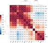 |
Fig. 5. Clustermap correlation for the 15 input features. The correlation matrix displays the numerical correlation coefficients in each cell, with a color scale ranging from −1 to 1, where 0 indicates no correlation (white), −1 indicates linear anticorrelation (blue), and 1 indicates linear correlation (red). The dendrogram reveals two main feature clusters: cluster A, composed of color indices, and cluster B, composed of morpho-parameters. |
Cluster A consists of color indices (photometric colors), several of which are strongly correlated. Within this cluster, two sub-clusters can be identified: one grouping the colors (i′−Ks) and (J − Ks), and another containing the remaining color indices. Cluster B comprises the morpho-parameters, which are also divided into two sub-clusters: one dominated by the concentration index, and another including the remaining morpho-parameters. Although some of the morphological parameters are highly correlated with each other, they remain largely uncorrelated with the photometric colors.
It is worth noting that the apparent anticorrelation between color and morphological size observed when the u′ band is included arises from its larger seeing, stronger PSF variability, and lower S/N (particularly for faint or extended sources) compared to the g′ and i′ bands. These effects artificially increase the measured structural parameters, while the mixture of populations (objects that are either bright or faint in the u′ band) naturally reinforces the observed trend.
Notably, the color (J − Ks) exhibits weaker correlations with other colors, suggesting that it may carry more independent information about the underlying stellar populations. This behavior may be linked to the advantages of including NIR filters, where the spectral energy distribution of individual stars or the integrated light of stellar systems (GCs or galaxies) is dominated by intermediate- to old-age populations, such as cool K- and M-type giant stars, as well as stars at the tip of the red giant branch or on the asymptotic giant branch (e.g., Verro et al. 2022).
We adopted a combined strategy of permutation feature importance to assess relevance and a correlation clustermap to identify redundancy so that we could maximize the information content, while minimizing feature overlap. Based on the permutation feature importance shown in Fig. 4 (bottom panel), we selected the most diagnostic features with a mean decrease in precision greater than 0.025. This criterion leads to the exclusion of ellipticity, (u′−J), (u′−Ks) and the concentration index. The clustermap in Fig. 5 further allows us to identify potentially redundant features.
Among the 11 remaining features, and taking into account the correlations discussed above, we retain the following seven parameters: SM, (J − Ks), (g′−i′), (i′−Ks), (u′−g′), (i′−J), and FWHM. The remaining features may either be excluded or tested individually to evaluate their impact on the model performance. Notably, all four of these excluded features show strong correlations with one or more of the selected features: (u′−i′) with (g′−i′) (corr = 0.91) and (u′−g′) (corr = 0.92); (g′−Ks) with (i′−Ks) (corr = 0.90); (g′−J) with (g′−i′) (corr = 0.95); and FR with FWHM (corr = 0.86) and SM (corr = 0.82).
In addition, we evaluated two reduced feature sets: a six-feature (6F) configuration, excluding FWHM, and a five-feature (5F) configuration, excluding both (i′−J) and FWHM. The svm.SVC models using the seven-feature (7F) configuration show improved classification performance, achieving a better balance between overfitting and overall scores compared to the other feature sets. Therefore, a combination of color indices spanning the NUV, optical, and NIR regimes, together with two structural parameters (SM and FWHM), provides the most effective and efficient class separation.
In the next section, we present additional tests to further assess the performance of the svm.SVC model. For the subsequent analysis, we adopted both the 15F and 7F configurations.
5. Performance and further tests of the svm.SVC classification model
In this section, we present the classification performance for two feature configurations: (i) the full 15F set and (ii) the reduced 7F set, derived using the combined dimensionality reduction strategy described in Sect. 4.5. The goal of this reduction is to improve model efficiency while mitigating overfitting and preserving classification accuracy.
Given that GCs, stars, and galaxies exhibit overlapping distributions in both the color space and morphological parameters, the classification task is inherently nonlinear. In this context, the RBF kernel is particularly effective, as it can model complex, nonlinear decision boundaries. Consistently, the GridSearchCV optimization procedure selects the RBF kernel as the best performing option across all tested configurations. The optimal hyperparameters for the best-performing 15F and 7F models correspond to C = 10 and γ = 0.1 or γ = scale, respectively.
5.1. Performance of the svm.SVC
It is important to emphasize that our svm.SVC model implementation is designed for deep photometric datasets and relies on color-based features, thereby avoiding the use of magnitudes, which are distance dependent. To construct a robust training and testing sample, the RV-confirmed GC population must extend to at least magi ≃ 22 in the i′ band, as GCs are the faintest objects among the three classes considered.
Within the RV-confirmed sample, we identify 447 GCs with magi ≤ 21 mag, 762 with magi ≤ 21.5 mag, and 1041 with magi ≤ 22 mag. To assess the impact of a shallower labeled sample, we test the 15F model under a hypothetical scenario in which the labeled data reach only magi = 21 mag (see Sect. 5.2). In addition, the code implemented in this study is computationally efficient, completing the full training, prediction, and classification workflow in under two minutes on a single CPU for a sky area of 3 deg2.
To evaluate the performance of the svm.SVC models, we used two standard metrics implemented in the scikit-learn library (Pedregosa et al. 2011). First, we employed the classification report, which provides per-class performance metrics for GCs, stars, and galaxies (see Table 2). This allowed us to compare the model performance across classes and to assess potential effects of class imbalance. Second, we used the normalized confusion matrix (Fawcett 2006), which illustrates how predictions are distributed among the true and predicted classes, thereby highlighting cases where the model tends to confuse one class with another.
Performance metrics used for model evaluation (Sokolova & Lapalme 2009).
Table 3 presents the classification report for the svm.SVC model trained using the full 15F set. Based on the precision values, the false-positive (FP) rates for the GC, star, and galaxy classes are 4.6%, 1.6%, and 2.8%, respectively. The recall values, which indicate the fraction of objects misclassified within each true class, are 3.0% for GCs, 1.9% for stars, and 3.6% for galaxies. Overall, the model correctly classifies 97.3% of the samples (1445 out of 1485).
For the dimensionality reduction described in Sect. 4.5, we adopt the 7F set: SM, (J − Ks), (g′−i′), (i′−Ks), (u′−g′), (i′−J), and FWHM. Table 4 presents the classification report for the svm.SVC model trained using this 7F configuration. Based on the precision values, the FP rates are 6.7% for GCs, 1.7% for stars, and 3.0% for galaxies. The recall values, remain high but are slightly lower than those obtained with the 15F model, reaching 96.1% for GCs, 97.2% for stars, and 96.2% for galaxies. The overall classification accuracy is 96.6%.
Classification Report for the 7F model, as the result of applying Permutation importance and clustermap correlation to remove features.
Although the 15F model yields marginally higher scores in the classification report, we attribute this difference to mild overfitting driven by redundant color indices and structural parameters. The 7F model therefore provides a more realistic and robust representation of the classification performance, as illustrated in Fig. 7.
The confusion matrices for the 15F and 7F models are shown in Fig. 6. Rows correspond to the true class labels, while columns correspond to the predicted class labels. Diagonal elements represent correct classifications, whereas off-diagonal elements indicate misclassifications. For a given class, false negatives (FN) correspond to objects of that class that are incorrectly assigned to another class (i.e., entries in the same row outside the diagonal), while FP correspond to objects predicted to belong to that class but whose true labels correspond to a different class (i.e., entries in the same column outside the diagonal).
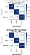 |
Fig. 6. Normalized confusion matrices with the true labels on the y-axis and the predicted labels on the x-axis. The svm.SVC results for the 15F and 7F models are shown in the top and bottom panels, respectively. |
Figure 6 (top panel) shows the normalized confusion matrix for the 15F model. Correct classification rates are 97.0%, 98.1%, and 96.4% for GCs, stars, and galaxies, respectively. The remaining misclassifications include GCs incorrectly classified as stars (0.8%) or galaxies (2.2%), stars misclassified as GCs (1.0%) or galaxies (0.8%), and galaxies misclassified as GCs (2.1%) or stars (1.5%), resulting in an overall misclassification rate of 8.4%.
Figure 6 (bottom panel) presents the normalized confusion matrix for the 7F model, which shows slightly lower classification performance compared to the 15F model. Correct classification rates are 96.1%, 97.2%, and 96.2% for GCs, stars, and galaxies, respectively, corresponding to a total misclassification rate of 10.4%.
The confusion matrix indicate that the 15F model yields higher performance metrics than the 7F model, however the analysis in Sect. 4.5 shows that four features contribute little to the classification and that several others are highly correlated with the most informative features. This suggests that the 7F configuration provides a more robust and interpretable representation of the underlying data, despite its marginally lower scores.
5.2. Testing the svm.SVC classifier using a magnitude-constrained train + test sample
This section presents the results of a hypothetical scenario in which the labeled sample extends only to magi = 21 mag. The performance of the 15F model under this magnitude constraint is shown in Fig. C.2. After applying the magnitude cut, the labeled sample comprises 447 GCs, 2150 stars, and 1539 galaxies, with class 1 (GCs) being the most strongly affected.
The main performance indicators are the per-class precision and recall values (Fig. C.2, right panel). For GCs, the FP fraction increases to 9.3%, compared to 4.6% in the case without a magnitude cut, while the misclassification rate rises more moderately to 5.2% (from 3.0%). In contrast, classes 2 (stars) and 3 (galaxies) exhibit only minor variations, with differences below 1% relative to the no magnitude cut scenario.
In summary, imposing a magnitude limit of magi = 21 mag leads to a measurable degradation in the ability of the svm.SVC model to identify GCs, reflected by increased FP and misclassification rates, corresponding to an additional ≈5% classification error relative to the no–magnitude-cut In contrast, the classification performance for stars and galaxies remains largely unchanged.
These results demonstrate that the 15F model critically depends on the inclusion of fainter, RV-confirmed GCs to adequately capture the intrinsic structure of the GC class in color space and to preserve robust separability from contaminant populations (stars and galaxies). Consequently, a sufficiently deep labeled sample is essential to achieve optimal GC classification performance.
5.3. Performance of the svm.SVC model in classifying the unlabeled NGFS-T1 catalog
Following the training and testing of the svm.SVC model, it was applied to assign predicted class labels to all sources in the NGFS-T1 input catalog. The predicted classes are encoded as GC = 1, Star = 2, and Galaxy = 3. Class predictions were obtained using the model.predict method, which returns the most likely class label for each source in the input dataset. In addition, we used model.predict_proba to retrieve the full class probability distribution for each source.
The majority of sources are classified with high confidence: 61% have a maximum predicted class probability ≥90%, and 92% exceed a probability threshold of ≥60%. The final catalog for the previously unlabeled sample provides a classification for every source, determined by the class with the highest predicted probability. Although no explicit probability threshold was applied to filter classifications, the model demonstrates robust performance across the full dataset.
Figure 7 shows the results of the svm.SVC classification applied to the unlabeled NGFS-T1 sample, comprising a total of 57 469 sources. The top panels present the results obtained with the 15F model, while the bottom panels show those from the 7F model. Each panel includes a title indicating the kernel, its hyperparameters, and the feature set used. The left column displays the u′i′Ks cc–diagram, and the second column shows the u′g′Ks diagram. These projections were selected because they clearly highlight the separation between the three target classes: GCs, foreground stars, and galaxies. The probability of each source being assigned to a given class is color-coded, ranging from red (50%) to blue (100%).
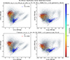 |
Fig. 7. Results of the svm.SVC model applied to the full NGFS-T1 catalog using the 15F (top panels) and 7F (bottom panels; see Sects. 4.4 and 5). The two cc–diagrams shown are u′i′Ks (first column) and u′g′Ks (second column). The color scale represents the model assigned probability of each source being classified as a GC, ranging from 50% (red) to 100% (blue). Probabilities are computed in the full feature space; therefore, these diagrams provide 2D projections intended solely for visualization purposes. |
It is important to note that the class probabilities are computed in the full multidimensional feature space. The cc–diagrams shown here serve solely as visual projections to illustrate class separation and do not reflect the complete decision boundaries of the model.
The classification results obtained with the 15F model yield 5350 GCs, 5646 stars, and 46 473 galaxies. Figure 7 displays the GC class probabilities using a color scale, where blue colors correspond to regions of high classification confidence. In comparison, the 7F model identifies 3960 globular clusters, 5831 stars, and 47 678 galaxies, indicating a reduction in the number of GC candidates relative to the 15F model. Nevertheless, the GC selection obtained with the 7F model exhibits a cleaner probability distribution, with fewer sources in the intermediate probability range (70–80%). This cleaner separation makes likely contaminants in the svm.SVC classification more apparent in the cc–diagrams.
Notably, GC candidates with lower probabilities that appear in the upper (redder) region of the galaxy locus are primarily associated with confusion with compact, high-redshift galaxies. This effect is consistent with the predictions from the PEGASE.2 population synthesis models shown in Fig. 3.
Based on the confusion matrices shown in Fig. 6, we estimate overall misclassification rates of 8.4% for the 15F model and 10.4% for the 7F model. Figure 7 illustrates that, despite the slightly better global scores achieved by the 15F model (see Sect. 5.1), the 7F model (built from the most relevant and least correlated features) appears to provide a more reliable and interpretable classification.
To further refined the selection of GC candidates obtained with the 7F model, we applied an additional constraint based on the model-assigned class probabilities. As shown in Fig. 7, sources with predicted GC probabilities below 80% tend to deviate from the GC locus and migrate toward the stellar or galactic regions in color–color space. Adopting a conservative probability threshold of 80%, we retained 1717 GC candidates from the unlabeled sample. Including the 1209 spectroscopically confirmed GCs (with RV measurements), the final GC catalog comprises a total of 2926 sources.
5.4. Testing svm.SVC model predictions with fewer filter information
The previous section presented results obtained using five filter photometry (u′g′i′JKs), achieving strong classification performance. In this section, we revisit the model to evaluate its behavior under more limited photometric coverage, specifically scenarios in which either the u′ band or the NIR bands are unavailable. The results are summarized in Fig. 8, which presents two cases: a six-feature (6F) model without the u′ band (top row), and a five-feature (5F) model using optical data only, i.e., without NIR information (bottom row).
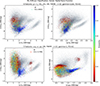 |
Fig. 8. Classification results of the svm.SVC model using different color configurations. Top row: model excluding the u′-band. Bottom row: model excluding the NIR bands. The left-column panels show the corresponding u′i′Ks cc–diagrams, while the right-column panels display cc–diagrams tailored to each model configuration: g′i′Ks for the top row and u′g′i′ for the bottom row. |
Figure 8 shows the classification results for the unlabeled NGFS-T1 catalog. In all cases, the left-column panels display the u′i′Ks cc–diagram for reference. The right-column panels show cc–diagrams constructed from the specific filters used by each model: g′i′Ks for the 6F model (no u′ band), and u′g′i′ for the 5F model (no NIR bands). The main results of this test are summarized below:
-
6F model: this configuration omits the u′-band information and uses the features (g′−i′), (i′−J), (i′−Ks), (J − Ks), SM, and FWHM. The classification report (Table C.1) and the confusion matrix shown in Fig. C.3 indicate precision and recall values of 93.0% and 95.3% for GCs, 97.7% and 96.9% for stars, and 97.3% and 96.4% for galaxies, yielding an overall accuracy of 96.4%. Despite this relatively high performance, the absence of u′-band data increases the number of FP, FN, and misclassifications across all classes. In Fig. 8, the top panels show the svm.SVC classification results for the 6F model, where GCs (class = 1) correspond to 4863 candidates. Significant confusion is evident, as many high probability GC candidates appear in regions of color–color space typically occupied by stars or galaxies. We note that, in practice, when u′ band data are unavailable, only the top-right panel (based on the available filters) should be used for interpretation.
-
5F model: this model excludes the NIR bands and uses the features (u′−g′), (u′−i′), (g′−i′), SM, and FWHM. The classification report (Table C.2) and the confusion matrix (Fig. C.3, bottom panel) show precision and recall values of 83.8% and 90.9% for GCs, 95.2% and 91.6% for stars, and 95.5% and 94.1% for galaxies. The overall accuracy decreases to 92.3%, accompanied by a substantial increase in confusion among the three classes. This behavior is evident in the cc–diagrams shown in the bottom panels of Fig. 8, and in the large number of GC candidates selected for class 1, totaling 11 786 objects.
Consequently, the inclusion of both NUV (u′) and NIR photometric data, in combination with standard optical bands, is essential for constructing an effective ML-based classification framework, such as the supervised SVM approach presented in this work. Our most reliable model is based on seven features (five colors and two morpho-parameters) and achieves an estimated contamination rate of ∼10.4%.
For comparison, González-Lópezlira et al. (2019) reported a contamination rate of ∼30% when using a single (u′−i′) versus (i′−Ks) cc–diagram. In their earlier study, González-Lópezlira et al. (2017) identified 39 GC candidates and estimated a total GC population of NGC = 144 ± 31 (random) ±38 (systematic) for the galaxy NGC 4258, assuming a contamination rate of only 5%. However, subsequent spectroscopic follow-up led to a revised estimate of NGC = 105 ± 26 ± 31, highlighting the significant impact of higher than previously anticipated contamination on the inferred GC population size.
5.5. svm.SVC Model Output Catalogs
As described in Sect. 5.3, the 7F svm.SVC model yields a total of 3960 GC candidates (see the bottom panels of Fig. 7). By applying an additional selection criterion of predicted GC probability ≥80% (retaining 1717 candidates) and including the spectroscopically confirmed GCs, we obtain a final GC sample of 2926 objects for the 7F model.
This final classification catalog produced by our model will serve as the foundation for a comprehensive analysis of the GC population in the NGFS-T1 field (cluster-centric radius ≤350 kpc), and will be presented in two forthcoming publications. The first will focus on GCs associated with the 279 galaxies identified by Eigenthaler et al. (2018), as well as on the intracluster GC population, using magnitudes, colors, full SED information, and spatial distributions across the cluster. The second study will investigate the stellar population properties, luminosity and mass functions of the GC system, and their scaling relations. The complete GC catalogs will be made publicly available as supplementary material accompanying the second publication. Catalogs of star and galaxy candidates will also be used in future follow-up studies led by the NGFS collaboration.
Figure 9 illustrates the quality of the final GC catalog, combining the SVM-based classification with the RV-confirmed sample. The left panel shows the projected spatial distribution of GCs, while the middle and right panels present the (g′−i′) color and i′ band magnitude distributions, respectively. The GC surface density peaks toward the central dominant galaxy NGC 1399, with additional concentrations around other bright cluster galaxies and a substantial population of intracluster GCs. These objects provide valuable tracers for studying the stellar assembly and evolutionary history of the central region of the Fornax galaxy cluster.
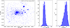 |
Fig. 9. Final GC catalog obtained from the svm.SVC classification model (7F), including spectroscopically RV-confirmed objects. Left panel: projected spatial distribution of GCs, with the highest densities concentrated around NGC 1399 and other massive galaxies. Middle panel: (g′−i′) color distribution. Right panel: i′-band magnitude distribution. |
In Appendix B.1, we summarize other ML methodologies used to select GCs and UCDs in the Fornax region and in other areas of the sky using photometric datasets. In addition, in Appendix B.2, we compare our svm.SVC GC sample with existing photometric catalogs, including the ACS Fornax Cluster Survey (Jordán et al. 2015), the Fornax Deep Survey (Cantiello et al. 2020), and the catalog presented by Saifollahi et al. (2021).
6. Testing the svm.SVC Method with the LSST filter system
In this section, we describe how we tested the performance of the svm.SVC classification model using photometry from the Vera C. Rubin Observatory Legacy Survey of Space and Time (LSST), which includes the u′g′r′i′z′Y bands. This test was designed to inform potential LSST users about the diagnostic power of cc–diagrams in this filter set and to assess whether a reliable classification of GCs in the Fornax cluster (or in similar environments at comparable distances), as well as stars and galaxies, would be feasible using LSST photometry alone.
For this experiment, we used NGFS data, which provide deep imaging in the u′, g′, and i′ bands. To complete an LSST-like filter set, we incorporated additional photometry from the Dark Energy Survey (DES) DR2 catalog (Abbott et al. 2021), obtained with the BLANCO/DECam instrument, the same facility used for NGFS observations. DES provides deep coverage in the g′r′i′z′Y bands, but does not include u′-band data. By combining NGFS u′g′i′ photometry with DES r′z′Y data, we construct a synthetic LSST-like dataset with full six-band coverage.
The cross-matched NGFS-T1 and DES DR2 catalog contains a total of 46 505 objects. The cc–diagram combinations constructed using the u′g′r′i′z′Y bands are shown in Figure 10. These diagrams demonstrate the strong diagnostic power of broad SED coverage from u′ to Y for distinguishing among the different object classes expected in future LSST deep imaging data.
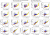 |
Fig. 10. Color-color diagrams for all sources with multiwavelength photometry in the core region of the Fornax galaxy cluster. Gray points show the full photometric sample, while colored points highlight spectroscopically confirmed objects: GCs (blue), stars (gold), and galaxies (purple; see Sect. 4.2). All diagrams display the same set of sources from the NGFS + DES DR2 cross-matched catalog, with photometric coverage in the u′g′r′i′z′Y bands (see Sect. 6). |
Among the tested combinations, the (u′−g′) versus (g′−Y) diagram (fourth column in the top row of Fig. 10) provides the clearest separation between the three main populations (GCs, stars, and galaxies). Nevertheless, GCs remain partially blended with the stellar locus. In the absence of near-UV u′ band data, the separation between classes degrades significantly, highlighting the critical role of the u′ band in effective photometric classification.
Using the same svm.SVC configuration applied to the u′g′i′JKs photometry, we cross-matched the labeled (training and test) sample with the u′g′r′i′z′Y dataset to construct an LSST-filter based feature set. Below, we present the classification results for three model configurations:
-
20-feature model (20F): Full filter coverage, including all u′g′r′i′z′Y bands and morpho-parameters (left column of Fig. 11 and its classification report in Table C.3);
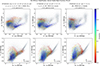
Fig. 11. Results of the svm.SVC model applied to the LSST filter system. The left-column panels show the 20F model (full u′g′r′i′z′Y coverage), the middle-column panels show the 12F model (excluding the u′ band), and the right-column panels show the 8F model (excluding both u′ and Y bands). The top-row panels display the u′g′Y cc–diagram, while the bottom-row panels show the g′i′z′ cc–diagram, representing the configuration without u′ and Y bands. The color scale indicates the classification probability assigned to each source, with higher values corresponding to greater confidence in the predicted class.
-
12-feature model (12F): Same configuration as the 20F model, but excluding the u′-band information (middle column of Fig. 11 and its classification report in Table C.4);
-
8-feature model (8F): Excludes both the u′ and Y bands (right column of Fig. 11 and its classification report in Table C.5).
In Fig. 11, the first column shows the u′g′Y cc– diagram, which provides the strongest discrimination among sources for the LSST-like filter set. The second column presents the g′i′z′ diagram, corresponding to the case in which both the u′ and Y bands are unavailable. Overall, the 20F model yields better classification performance than the 12F and 8F models.
The precision (purity) for GCs – the class most affected by selection biases – is systematically lower in the LSST-based tests, indicating an increased number of false positives compared to models that include NIR information. For the 20F model, the FP rate is 7.8%, rising to 8.3% and 10% for the 12F and 8F models, respectively. The 12F model, which excludes the u′ band (middle panels), classifies an excess number of sources as GCs, resulting in an increased population of high-probability objects extending into the stellar and galactic regions.
When the classification relies solely on g′r′i′z′ photometry, the cc–diagrams in the bottom-right panel exhibit substantial source mixing, particularly within the galaxy locus. It is worth noting that in the absence of both u′ and Y band data, only the right-column panels would be available for interpretation, in which case no clear separation among the three object classes can be achieved. This highlights the limitations imposed by reduced filter coverage.
These results underscore that robust photometric classification using the LSST filter system alone critically depends on the availability and depth of the u′ and Y bands. The full six-filter set substantially improves class separation, particularly when complemented by NIR data. For example, space-based missions such as Euclid, which is already operational, and the upcoming Nancy Grace Roman Space Telescope, will provide essential NIR coverage. Euclid is expected to overlap with LSST across approximately 7000 deg2 of the southern sky (Euclid Collaboration: Mellier et al. 2025a), offering an excellent opportunity to combine optical and NIR data.
Such joint datasets will enable classification methodologies, such as the one presented here to perform significantly better, especially in distinguishing compact stellar systems from background galaxies. Furthermore, the overlapping survey area will be critical for maximizing the scientific return of photometric classification efforts in large-scale extragalactic surveys.
7. Summary and future work
We have developed a supervised machine learning classifier based on an SVM (implemented using scikit-learn, svm.SVC) to distinguish between GCs, stars, and galaxies using deep photometric data from the central tile of the Next Generation Fornax Survey (Muñoz et al. 2015; Eigenthaler et al. 2018). The model leverages both optical (u′g′i′) and NIR (JKs) filters to construct color indices. Among the cc-diagrams, the most discriminating combinations are (u′−g′) versus (g′−Ks) (referred to as u′g′Ks), as well as u′i′Ks, u′JKs, and g′JKs, for identifying the three object types. In addition to the individual color indices, we included morphological parameters such as the FWHM, SM, concentration index, ellipticity, and FR to enhance the class separation (see Sect. 4.5).
The model was trained and tested using a set of spectroscopically confirmed sources within the same field of view: 1209 confirmed GCs, 2151 foreground stars, and 1587 galaxies (see Sect. 4.2). Our results demonstrate that broad spectral energy distribution coverage, particularly spanning the NUV to NIR, is essential for achieving high classification accuracy and minimizing confusion between compact stellar systems and background galaxies.
The optimized 7F model, which incorporates the key color indices and structural parameters, demonstrates the most reliable performance, achieving 96.6% accuracy and a misclassification rate of 10.4%. Although the full 15F model obtained higher scores in the classification report, we show that some features are irrelevant and a few others are redundant, including the (u′−i′) color, which is correlated with (u′−g′) and (g′−i′) – features with higher importance for the svm.SVC model. This difference in scores likely results from overfitting. The 7F model additionally provides computational efficiency, making it a more practical choice for large-scale applications.
In contrast, models trained on reduced filter sets, particularly those lacking near-UV (u′) and NIR (JKs) data, exhibit substantially degraded performance. Simulations using LSST-like filters (u′g′r′i′z′Y) indicate that the u′ and Y bands are essential for achieving acceptable classification accuracy, although even with their inclusion, performance remains inferior to models incorporating NIR coverage.
These results highlight the diagnostic power of broad spectral energy distribution coverage, spanning the near-UV to the NIR, especially when combined with basic morphological parameters. The final classification catalog produced by our model will serve as the foundation for a detailed statistical analysis of the globular cluster population in the core of the Fornax cluster (Ordenes-Briceño et al., in prep.).
Looking ahead, the integration of data from upcoming space-based missions, such as Euclid and the Nancy Grace Roman Space Telescope, will further enhance photometric classification capabilities across large sky areas, particularly in synergy with ground-based surveys such as LSST.
Acknowledgments
Y. Ordenes-Briceño acknowledges support from the FONDECYT Postdoctorado 2021 No. 3210442 and ESO comité mixto 2024. T.H. Puzia gratefully acknowledges support through FONDECYT Regular No. 1201016. T.H. Puzia, E.J. Johnston and P.K. Nayak acknowledge the support from the ANID CATA-BASAL project FB210003. J.P. Carvajal and R. Rahatgaonkar gratefully acknowledge support from ANID Beca Doctorado Nacional. This research has made use of the NASA/IPAC Extragalactic Database, which is funded by the National Aeronautics and Space Administration and operated by the California Institute of Technology. The authors deeply thank the citizens of Chile for their tax contributions to the national development of science and this project in these difficult post-pandemic times. The authors extend their gratitude to the researchers whose studies have been instrumental for this work. Facilities: CTIO (4 m Blanco/DECam), ESO:VISTA. Software:NumPY/Python3 v2.1.0; Pandas/Python3 v2.2.2; Scipy/Python3 v1.14.1; Sklearn/Python3 (v.1.5.1 Pedregosa et al. 2011) Astropy/Python3 v6.1.2 (v6.1.2 Astropy Collaboration 2013, 2018, 2022); Matplotlib/Python3 (v3.9.2 Hunter 2007); Seaborn/Python3 (v0.13.2 Waskom 2021); TopCat (Taylor 2005).
References
- Abbott, T. M. C., Adamów, M., Aguena, M., et al. 2021, ApJS, 255, 20 [NASA ADS] [CrossRef] [Google Scholar]
- Alamo-Martínez, K. A., Blakeslee, J. P., Jee, M. J., et al. 2013, ApJ, 775, 20 [CrossRef] [Google Scholar]
- Anand, G. S., Tully, R. B., Cohen, Y., et al. 2024, ApJ, 973, 83 [Google Scholar]
- Angora, G., Brescia, M., Cavuoti, S., et al. 2019, MNRAS, 490, 4080 [CrossRef] [Google Scholar]
- Ashman, K. M., & Zepf, S. E. 1992, ApJ, 384, 50 [Google Scholar]
- Astropy Collaboration (Robitaille, T. P., et al.) 2013, A&A, 558, A33 [NASA ADS] [CrossRef] [EDP Sciences] [Google Scholar]
- Astropy Collaboration (Price-Whelan, A. M., et al.) 2018, AJ, 156, 123 [Google Scholar]
- Astropy Collaboration (Price-Whelan, A. M., et al.) 2022, ApJ, 935, 167 [NASA ADS] [CrossRef] [Google Scholar]
- Barbisan, E., Huang, J., Dage, K. C., et al. 2022, MNRAS, 514, 943 [NASA ADS] [CrossRef] [Google Scholar]
- Bergond, G., Athanassoula, E., Leon, S., et al. 2007, A&A, 464, L21 [NASA ADS] [CrossRef] [EDP Sciences] [Google Scholar]
- Bertin, E. 2006, ASP Conf. Ser., 351, 112 [NASA ADS] [Google Scholar]
- Bertin, E. 2011, ASP Conf. Ser., 442, 435 [Google Scholar]
- Bertin, E., & Arnouts, S. 1996, A&AS, 117, 393 [NASA ADS] [CrossRef] [EDP Sciences] [Google Scholar]
- Bertin, E., Mellier, Y., Radovich, M., et al. 2002, ASP Conf. Ser., 281, 228 [Google Scholar]
- Blanton, M. R., & Roweis, S. 2007, AJ, 133, 734 [NASA ADS] [CrossRef] [Google Scholar]
- Breiman, L. 2001, Mach. Learn., 45, 5 [Google Scholar]
- Brodie, J. P., & Strader, J. 2006, ARA&A, 44, 193 [Google Scholar]
- Cantiello, M., Venhola, A., Grado, A., et al. 2020, A&A, 639, A136 [NASA ADS] [CrossRef] [EDP Sciences] [Google Scholar]
- Cenarro, A. J., Moles, M., Cristóbal-Hornillos, D., et al. 2019, A&A, 622, A176 [NASA ADS] [CrossRef] [EDP Sciences] [Google Scholar]
- Chapelle, O., Vapnik, V., Bousquet, O., & Mukherjee, S. 2002, Mach. Learn., 46, 131 [Google Scholar]
- Chaturvedi, A., Hilker, M., Cantiello, M., et al. 2022, A&A, 657, A93 [NASA ADS] [CrossRef] [EDP Sciences] [Google Scholar]
- Chen, Y., Mo, H., & Wang, H. 2025, MNRAS, 540, 1235 [Google Scholar]
- Chies-Santos, A. L., de Souza, R. S., Caso, J. P., et al. 2022, MNRAS, 516, 1320 [Google Scholar]
- Chilingarian, I. V., Mieske, S., Hilker, M., & Infante, L. 2011, MNRAS, 412, 1627 [NASA ADS] [CrossRef] [Google Scholar]
- Cooper, A. P., Frenk, C. S., Hellwing, W. A., & Bose, S. 2025, MNRAS, 540, 2049 [Google Scholar]
- Cortes, C., & Vapnik, V. 1995, Mach. Learn., 20, 273 [Google Scholar]
- Crammer, K., & Singer, Y. 2002, J. Mach. Learn. Res., 2, 265 [Google Scholar]
- Cristiani, S., Grazian, A., Omizzolo, A., & Corbally, C. 2001, in Mining the Sky, eds. A. J. Banday, S. Zaroubi, & M. Bartelmann, 154 [Google Scholar]
- Drinkwater, M. J., Phillipps, S., Jones, J. B., et al. 2000, A&A, 355, 900 [NASA ADS] [Google Scholar]
- Drinkwater, M. J., Gregg, M. D., & Colless, M. 2001, ApJ, 548, L139 [Google Scholar]
- Durrell, P. R., Côté, P., Peng, E. W., et al. 2014, ApJ, 794, 103 [NASA ADS] [CrossRef] [Google Scholar]
- Eigenthaler, P., Puzia, T. H., Taylor, M. A., et al. 2018, ApJ, 855, 142 [Google Scholar]
- Euclid Collaboration (Mellier, Y., et al.) 2025a, A&A, 697, A1 [Google Scholar]
- Euclid Collaboration (Voggel, K., et al.) 2025b, A&A, 693, A251 [Google Scholar]
- Fahrion, K., Lyubenova, M., Hilker, M., et al. 2020, A&A, 637, A26 [NASA ADS] [CrossRef] [EDP Sciences] [Google Scholar]
- Fawcett, T. 2006, Pattern Recognit. Lett., 27, 861 [Google Scholar]
- Ferguson, H. C. 1989, AJ, 98, 367 [Google Scholar]
- Ferrarese, L., Côté, P., Cuillandre, J.-C., et al. 2012, ApJS, 200, 4 [Google Scholar]
- Fioc, M., & Rocca-Volmerange, B. 1997, A&A, 326, 950 [NASA ADS] [Google Scholar]
- Fitzpatrick, E. L. 1999, PASP, 111, 63 [Google Scholar]
- Flaugher, B., Diehl, H. T., Honscheid, K., et al. 2015, AJ, 150, 150 [Google Scholar]
- Forbes, D. A., Brodie, J. P., & Grillmair, C. J. 1997, AJ, 113, 1652 [Google Scholar]
- Forbes, D. A., Read, J. I., Gieles, M., & Collins, M. L. M. 2018, MNRAS, 481, 5592 [NASA ADS] [CrossRef] [Google Scholar]
- Gaia Collaboration (Brown, A. G. A., et al.) 2021, A&A, 649, A1 [NASA ADS] [CrossRef] [EDP Sciences] [Google Scholar]
- Georgiev, I. Y., Puzia, T. H., Goudfrooij, P., & Hilker, M. 2010, MNRAS, 406, 1967 [NASA ADS] [Google Scholar]
- González-Lópezlira, R. A., Lomelí-Núñez, L., Álamo-Martínez, K., et al. 2017, ApJ, 835, 184 [CrossRef] [Google Scholar]
- González-Lópezlira, R. A., Mayya, Y. D., Loinard, L., et al. 2019, ApJ, 876, 39 [Google Scholar]
- Gregg, M. D., Drinkwater, M. J., Evstigneeva, E., et al. 2009, AJ, 137, 498 [NASA ADS] [CrossRef] [Google Scholar]
- Guyon, I., Weston, J., Barnhill, S., & Vapnik, V. 2002, Mach. Learn., 46, 389 [Google Scholar]
- Harris, W. E., & Reina-Campos, M. 2024, ApJ, 971, 155 [Google Scholar]
- Harris, W. E., Harris, G. L. H., & Alessi, M. 2013, ApJ, 772, 82 [Google Scholar]
- Hilker, M., Infante, L., Vieira, G., Kissler-Patig, M., & Richtler, T. 1999, A&AS, 134, 75 [NASA ADS] [CrossRef] [EDP Sciences] [Google Scholar]
- Hilker, M., Baumgardt, H., Infante, L., et al. 2007, A&A, 463, 119 [NASA ADS] [CrossRef] [EDP Sciences] [Google Scholar]
- Huertas-Company, M., Rouan, D., Tasca, L., Soucail, G., & Le Fèvre, O. 2008, A&A, 478, 971 [NASA ADS] [CrossRef] [EDP Sciences] [Google Scholar]
- Hunter, J. D. 2007, Comput. Sci. Eng., 9, 90 [NASA ADS] [CrossRef] [Google Scholar]
- Ivezić, Ž., Kahn, S. M., Tyson, J. A., et al. 2019, ApJ, 873, 111 [Google Scholar]
- Joachims, T. 1998, Lect. Notes Comput. Sci., 1398, 137 [Google Scholar]
- Jordán, A., Peng, E. W., Blakeslee, J. P., et al. 2015, ApJS, 221, 13 [Google Scholar]
- Kissler-Patig, M., Grillmair, C. J., Meylan, G., et al. 1999, AJ, 117, 1206 [CrossRef] [Google Scholar]
- Kluge, M., Hatch, N. A., Montes, M., et al. 2025, A&A, 697, A13 [NASA ADS] [CrossRef] [EDP Sciences] [Google Scholar]
- Li, G., Lu, Z., Wang, J., & Wang, Z. 2025, ArXiv e-prints [arXiv:2502.15300] [Google Scholar]
- Lim, S., Peng, E. W., Côté, P., et al. 2024, ApJ, 966, 168 [NASA ADS] [CrossRef] [Google Scholar]
- Lim, S., Peng, E. W., Côté, P., et al. 2025, ApJS, 276, 34 [Google Scholar]
- Liu, Q., Chen, C., Zhang, Y., & Hu, Z. 2011, Artif. Intell. Rev., 36, 99 [Google Scholar]
- Maddox, N., Serra, P., Venhola, A., et al. 2019, MNRAS, 490, 1666 [Google Scholar]
- Madrid, J. P., O’Neill, C. R., Gagliano, A. T., & Marvil, J. R. 2018, ApJ, 867, 144 [NASA ADS] [CrossRef] [Google Scholar]
- Małek, K., Solarz, A., Pollo, A., et al. 2013, A&A, 557, A16 [NASA ADS] [CrossRef] [EDP Sciences] [Google Scholar]
- Maschmann, D., Lee, J. C., Thilker, D. A., et al. 2024, ApJS, 273, 14 [Google Scholar]
- Mieske, S., Hilker, M., & Infante, L. 2002, A&A, 383, 823 [CrossRef] [EDP Sciences] [Google Scholar]
- Mieske, S., Hilker, M., & Infante, L. 2004, A&A, 418, 445 [NASA ADS] [CrossRef] [EDP Sciences] [Google Scholar]
- Mieske, S., Hilker, M., Jordán, A., et al. 2008, A&A, 487, 921 [NASA ADS] [CrossRef] [EDP Sciences] [Google Scholar]
- Mohammadi, M., Mutatiina, J., Saifollahi, T., & Bunte, K. 2022, Astron. Comput., 39, 100555 [NASA ADS] [CrossRef] [Google Scholar]
- Muñoz, R. P., Puzia, T. H., Lançon, A., et al. 2014, ApJS, 210, 4 [Google Scholar]
- Muñoz, R. P., Eigenthaler, P., Puzia, T. H., et al. 2015, ApJ, 813, L15 [Google Scholar]
- Ordenes Briceño, Y. 2018, Ph.D. Thesis, Ruprecht-Karls University of Heidelberg, Germany [Google Scholar]
- Ordenes-Briceño, Y., Eigenthaler, P., Taylor, M. A., et al. 2018, ApJ, 859, 52 [Google Scholar]
- Pedregosa, F., Varoquaux, G., Gramfort, A., et al. 2011, J. Mach. Learn. Res., 12, 2825 [Google Scholar]
- Peng, E. W., Jordán, A., Côté, P., et al. 2006, ApJ, 639, 95 [Google Scholar]
- Peng, E. W., Ferguson, H. C., Goudfrooij, P., et al. 2011, ApJ, 730, 23 [Google Scholar]
- Pfeffer, J., Kruijssen, J. M. D., Crain, R. A., & Bastian, N. 2018, MNRAS, 475, 4309 [Google Scholar]
- Platt, J. C. 1999a, Fast Training of Support Vector Machines Using Sequential Minimal Optimization (Cambridge, MA, USA: MIT Press), 185 [Google Scholar]
- Platt, J. C. 1999b, Advances in Large Margin Classifiers (MIT Press), 61 [Google Scholar]
- Pota, V., Napolitano, N. R., Hilker, M., et al. 2018, MNRAS, 481, 1744 [Google Scholar]
- Powalka, M., Lançon, A., Puzia, T. H., et al. 2016, ApJS, 227, 12 [Google Scholar]
- Puzia, T. H., Kissler-Patig, M., Thomas, D., et al. 2005, A&A, 439, 997 [NASA ADS] [CrossRef] [EDP Sciences] [Google Scholar]
- Puzia, T. H., Kissler-Patig, M., & Goudfrooij, P. 2006, ApJ, 648, 383 [NASA ADS] [CrossRef] [Google Scholar]
- Puzia, T. H., Paolillo, M., Goudfrooij, P., et al. 2014, ApJ, 786, 78 [Google Scholar]
- Saifollahi, T., Janz, J., Peletier, R. F., et al. 2021, MNRAS, 504, 3580 [NASA ADS] [CrossRef] [Google Scholar]
- Saifollahi, T., Voggel, K., Lançon, A., et al. 2025, A&A, 697, A10 [NASA ADS] [CrossRef] [EDP Sciences] [Google Scholar]
- Schlafly, E. F., & Finkbeiner, D. P. 2011, ApJ, 737, 103 [Google Scholar]
- Schlegel, D. J., Finkbeiner, D. P., & Davis, M. 1998, ApJ, 500, 525 [Google Scholar]
- Schuberth, Y., Richtler, T., Hilker, M., et al. 2010, A&A, 513, A52 [NASA ADS] [CrossRef] [EDP Sciences] [Google Scholar]
- Shi, F., Liu, Y.-Y., Sun, G.-L., et al. 2015, MNRAS, 453, 122 [Google Scholar]
- Skrutskie, M. F., Cutri, R. M., Stiening, R., et al. 2006, AJ, 131, 1163 [NASA ADS] [CrossRef] [Google Scholar]
- Smith, R., Sánchez-Janssen, R., Beasley, M. A., et al. 2015, MNRAS, 454, 2502 [Google Scholar]
- Sokolova, M., & Lapalme, G. 2009, Inf. Process. Manage., 45, 427 [Google Scholar]
- Sutherland, W., Emerson, J., Dalton, G., et al. 2015, A&A, 575, A25 [NASA ADS] [CrossRef] [EDP Sciences] [Google Scholar]
- Taylor, M. B. 2005, ASP Conf. Ser., 347, 29 [Google Scholar]
- Taylor, M. A., Puzia, T. H., Muñoz, R. P., et al. 2017, MNRAS, 469, 3444 [NASA ADS] [CrossRef] [Google Scholar]
- Ting, Y. S., Nguyen, T. D., Ghosal, T., et al. 2025, Astron. Comput., 51, 100893 [Google Scholar]
- Usher, C., Dage, K. C., Girardi, L., et al. 2023, PASP, 135, 074201 [NASA ADS] [CrossRef] [Google Scholar]
- Valdes, F., Gruendl, R., & DES Project. 2014, ASP Conf. Ser., 485, 379 [NASA ADS] [Google Scholar]
- Vandenberg, D. A., Bolte, M., & Stetson, P. B. 1996, ARA&A, 34, 461 [NASA ADS] [CrossRef] [Google Scholar]
- Vavilova, I. B., Dobrycheva, D. V., Vasylenko, M. Y., et al. 2021, A&A, 648, A122 [NASA ADS] [CrossRef] [EDP Sciences] [Google Scholar]
- Verro, K., Trager, S. C., Peletier, R. F., et al. 2022, A&A, 661, A50 [NASA ADS] [CrossRef] [EDP Sciences] [Google Scholar]
- Wang, C., Bai, Y., López-Sanjuan, C., et al. 2022, A&A, 659, A144 [Google Scholar]
- Waskom, M. L. 2021, J. Open Source Softw., 6, 3021 [CrossRef] [Google Scholar]
- Willman, B., & Strader, J. 2012, AJ, 144, 76 [Google Scholar]
Figure 5 may be particularly useful in cases with limited filter coverage, as it highlights highly correlated feature pairs (correlation > 0.9) and suggests optimal feature combinations for constructing effective SVM models.
Appendix A: Photometric calibration for NGFS-T1
In this section, we present a brief overview of the data reduction process for the central Fornax region (3 deg2 in the DECam FoV. A complete description of the NGFS survey data reduction will be presented in a dedicated paper.
A.1. Data processing
For the optical data, the raw DECam images were processed using the DECam Community Pipeline (v3.4.0; Valdes et al. 2014), which corrects for bias, flat fielding, and image crosstalk, thereby removing instrumental signatures (InstCal FITS files). We then applied a custom background subtraction strategy, followed by astrometric calibration, photometric calibration, and image stacking using SCAMP (v2.2.6; Bertin 2006), Source Extractor (SE, v2.19.5; Bertin & Arnouts 1996), and SWARP (v2.19.5; Bertin et al. 2002), respectively. For the astrometric calibration, we employed SDSS Stripe 82 standard stars, and color-term corrections were applied to each source after photometry. The optical-band photometry in the g′ and i′ filters was cross-checked against the Dark Energy Survey DR2 (Abbott et al. 2021) and complemented with data from the Fornax Deep Survey (Cantiello et al. 2020).
The central NIR region (VIRCam T1 and T2, overlapping) was previously processed in Ordenes Briceño (2018). The VISTA data in J and Ks filters were reduced from scratch using a pipeline similar to that for the optical data, but with a modified sky modeling function to account for the highly variable NIR sky. Atmospheric emission, primarily from water vapor and OH molecules, causes rapid sky fluctuations on short timescales, making sky subtraction a critical step in NIR image processing. Astrometric and photometric calibration for the NIR data were performed using reference stars from the 2MASS Point Source Catalog (Skrutskie et al. 2006).
Figure A.1 shows the results of our photometric calibration, compared with the optical and NIR surveys mentioned above. We cross-matched the NGFS catalog (u′g′i′JKs) with Gaia DR3 (Gaia Collaboration 2021). For the Gaia catalog, we imposed a declination uncertainty of ≤0.5 milliarcsec. For the NGFS optical catalog, we applied the following selection criteria: a SPREAD MODEL uncertainty (measured in the u′ band) < 0.00015 and FLAGS = 0. The u′ band FWHM exhibits the poorest image quality among the optical bands, primarily due to the lower throughput of the filter.
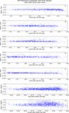 |
Fig. A.1. NGFS-Gaia DR3 cross-match. Comparison of PSF photometry with other surveys from the literature: the Fornax Deep Survey (Cantiello et al. 2020) in the u′ band (panel A), g′ band (panel B), and i′ band (panel D); the Dark Energy Survey (Abbott et al. 2021) in the g′ band (panel C) and i′ band (panel E); and 2MASS (Skrutskie et al. 2006) in the J band (panel F) and Ks band (panel G). |
A.2. Point-like source detection image
The central region of the Fornax Cluster is extremely rich in galaxies (see Fig. 1). Their extended surface brightness profiles hinder source detection, as many faint objects are embedded in or obscured by diffuse galaxy light. To improve the detection of point sources in the science images, we developed an iterative procedure based on SExtractor and its check images to construct a detection image that is as free as possible of the dominant galaxy light components.
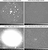 |
Fig. A.2. NGFS-T1 i′ band image. Left: Science image. Right: Result of the "point source" detection image. |
The procedure consists of two phases. In the first phase, we run SExtractor on the original image and use the BACKGROUND check image to identify diffuse light from the brightest galaxies and other extended components. This information is used to construct a diffuse light map, which is then subtracted from the original image. Several iterations are required; in our case, five iterations were sufficient to produce homogeneous sky backgrounds around sources and to significantly reduce galaxy halos.
The second phase involves an iterative median-filtering step. Using the output image from the first phase together with the OBJECT check image, we mask all detected point sources. The masked image is then subtracted from the first-phase output, leaving only unmasked extended structures, which are subsequently removed via median filtering. We apply a median filter with a kernel size of 21 pixels, which provides a good compromise between filtering efficiency and computational cost, given the large size of the DECam images (∼3 deg2). This process is repeated until only point sources remain, with no residual extended halos.
We repeat this procedure for each band image and then run SExtractor on the final processed images. The resulting catalogs are subsequently used as input to extract photometry for previously hindered sources when running SExtractor on the original science images (see Sect. 2).
Appendix B: Literature comparison with svm.SVC methodology and GC sample
B.1. Machine-learning methodologies in the literature
We have shown that machine-learning methodologies are essential for identifying extragalactic globular clusters (GCs) in wide-field surveys, overcoming the intrinsic difficulty of distinguishing them from contaminant populations, which can lead to contamination levels of 30–70% in purely optical samples. Previous studies emphasize the necessity of broad spectral coverage, combining optical and NIR filters, such as the u′ and Ks bands, to maximize the separation power.
In this work, we applied a supervised SVM classification method to NGFS-T1 data, trained on 1 209 spectroscopically confirmed GCs, 2 151 foreground stars, and 1 587 galaxies. The optimal reduced 7F SVM model achieved excellent performance on the test set, with a GC completeness (recall) of 96.1%, a GC purity (precision) of 93.3%, and an overall accuracy of 96.6%. Applying an additional probability threshold of ≥80% to the svm.SVC predictions yields 1 717 GC candidates from a total of 3 960 sources classified as GCs. When combined with the spectroscopically confirmed objects, this results in a final GC catalog containing 2 916 sources.
Focusing on the Fornax cluster environment, previous ML efforts include unsupervised clustering based on the Growing Neural Gas (GNG) algorithm (Angora et al. 2019). Using a training sample of 357 confirmed GCs, this approach achieved a GC completeness of 90.8% and a purity of 80.0%, with an overall accuracy of 86.5% (referred to as the average efficiency, AE) in a three-class classification problem, and identified approximately 522 GC candidates. Subsequent supervised approaches, such as the K-nearest neighbors method (KNN+100; Saifollahi et al. 2021), were trained on 137 pre-selected GCs and achieved a GC recall of 81% and a precision of 77% during cross-validation. This method ultimately identified 1 155 UCD/GC candidates.
More recent studies employing supervised classifiers, including Localized General Matrix Learning Vector Quantization (LGMLVQ) and Random Forest (RF; Mohammadi et al. 2022), used training samples of 512 confirmed GCs and reported strong performance, with GC recall exceeding 96.3%, GC precision above 93.5%, and an overall accuracy of 98.2%.
Other classification approaches include RF and Neural Network (NN) methods applied to the Virgo cluster (Barbisan et al. 2022). Trained on a sample of 1 243 spectroscopically confirmed UCDs and GCs, these models achieved up to 99.4% overall accuracy, with a combined GCs+UCDs precision of 98.9% and a recall of 99.2%. In a different context, a specialized statistical pipeline based on Principal Component Analysis (PCA) was applied to the M81/M82 group (Chies-Santos et al. 2022). Despite being trained on only 73 known GCs, this approach identified 642 new GC candidates.
These studies universally address the challenge of highly imbalanced datasets through strategies such as oversampling, two-step filtering or pre-selection to balance the training sample, or trimming the majority classes. In this work, we instead adopt an undersampling approach for the majority classes. Moreover, unlike some previous studies that exploit distance-dependent absolute magnitudes - typically applicable only to galaxies at similar distances - or apparent magnitude based variants to mitigate specific contaminants, our methodology relies exclusively on distance-independent colors and morphological parameters. This approach is particularly advantageous for wide-area surveys such as LSST, as colors robustly trace intrinsic stellar population properties, including age and metallicity.
B.2. svm.SVC GC sample and comparison with existing photometric catalogs
In the Fornax cluster region, several photometric catalogs of GC candidates have been produced by different surveys, each employing distinct methodologies and filter sets. For reference, our svm.SVC GC catalog contains 3 960 objects, of which 1 717 have a classification probability ≥80%. The full catalog, which combines the svm.SVC predictions with RV confirmed GCs, comprises 5 169 objects, with 2 926 sources having prob ≥ 80%. Below, we present a comparison with previous studies.
-
Cantiello et al. (2020): The Fornax Deep Survey, which selected GC candidates using u′g′r′i′ photometry, provides the catalog FDS_master_gc-ucd.dat containing 3 331 sources. Within the same central region considered in this work, 2 411 of these are GC candidates (prior to cross-matching). The cross-match yields 375 sources in common with our svm.SVC catalog and 1 369 sources in common with our full catalog with prob ≥ 80%.
-
Saifollahi et al. (2021): The Fornax Deep Survey combined with NIR imaging (u′g′r′i′JKs), using a ML method (KNN+100; see Sect. B.1), provides the catalog ucd_gc_candidates.fits containing 1 155 sources, 453 of which lie within the NGFS-T1 FoV. The comparison with our svm.SVC catalog and with the full catalog yields 186 and 251 sources in common, respectively.
-
Jordán et al. (2015): The HST/ACS Fornax Cluster Survey observed 43 galaxies and measured photometry in the F475W (Sloan g) and F850LP (Sloan z) filters. The excellent spatial resolution of HST/ACS allows reliable measurements of half-light radii, which are a key discriminator for separating GCs from contaminants when only a limited number of filters are available. For each source, a GC probability was estimated using a model-based mixture approach. The catalog ACSFCS_gz.dat contains a total of 9 136 sources and represents a highly reliable photometric dataset. Within the FoV of this work, only 14 ACSFCS galaxies are covered. Applying the same probability threshold of 80% used in our analysis, 3 052 sources satisfy this criterion. The cross-match between the ACSFCS catalog and our catalogs is sensitive to astrometric offsets, as we identified a systematic coordinate shift between ACSFCS and NGFS-T1/FDS. This was verified by overlaying our catalogs with FDS and ACSFCS sources on the NGFS-T1 i′ band image. To account for this offset, we adopted a matching radius of 2″ instead of the standard 1″. The resulting cross-match yields 346 sources in common with our svm.SVC catalog and 564 sources in common with the full catalog. The relatively small overlap (from 3 052 to fewer than 600 sources) is likely driven by the ACSFCS selection being based solely on g and z photometry, whereas our selection uses the broader u′g′i′JKs filter set. This limits our ability to recover ACSFCS sources in the shallowest bands, particularly u′ and Ks. In addition, many objects that are well detected in HST/ACS appear faint in our ground-based data, leading to low-quality photometry and their exclusion from the svm.SVC model. A further contributing factor is that ACSFCS detects sources very close to galaxy centers, whereas in our ground-based images the innermost regions are often saturated and cannot be reliably analyzed.
Appendix C: Additional tables and plots for testing the svm.SVC model
C.1. Testing the svm.SVC model with different split train+test samples, continued
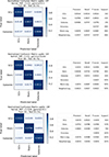 |
Fig. C.1. Different splits of the labeled training–testing sample. Left: Normalized confusion matrices. Right: Corresponding classification reports. The splits are 80%/20% (top row), 60%/40% (middle row), and 50%/50% (bottom row). The subtitles of the left panels indicate the kernel type and model parameters. |
Classification report for the 6F model, no u′ band: (g′−i′), (i′−J), (i′−Ks), (J − Ks), SM, and FWHM. See Sect. 5.4 and Fig. 8 (top row).
Classification report for the 5F model, no NIR: (u′−g′), (u′−i′), (g′−i′), SM, and FWHM. See Sect. 5.4 and Fig. 8 (bottom row).
In Sect. 4.4, we discussed the importance of achieving optimal validation performance and emphasized that a key factor is the random division of the labeled sample into training and testing subsets (using train_test_split). We explored several split configurations and found that the best performance is obtained with a 70% training and 30% testing split. In this section, we present the results for the alternative configurations, namely 80%/20%, 60%/40%, and 50%/50%, which are shown in Fig. C.1.
C.2. Testing the svm.SVC classifier using a magnitude-constrained train+test sample, continued
This section presents the results of a hypothetical test in which the labeled sample is limited to magi ≤ 21 mag. The performance of the 15F model under this magnitude constraint is shown in Fig. C.2; see Sect. 5.2 for further details.
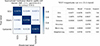 |
Fig. C.2. Performance of the 15F model evaluated on the labeled training–testing sample restricted to magi ≤ 21 mag. Left: Normalized confusion matrices. Right: Corresponding classification reports. The subtitles in the left panels specify the kernel type and model parameter configuration. |
C.3. Testing the svm.SVC model with fewer filter information, continued
This section presents complementary information for the cases in which fewer filters are used in the svm.SVC model; see Sect. 5.4 for details. The corresponding confusion matrices are shown in Fig. C.3, and the classification report tables are provided in Tables C.1 and C.2.
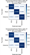 |
Fig. C.3. Normalized confusion matrix for the 6F (no u′ band) and 5F (no NIR) test models shown in the top and bottom panel, respectively. See Section 5.4 |
C.4. Application: Testing the method for LSST filter system, continued
The following tables (C.3, C.4, and C.5) show the classification report for the three models with different features, see Section 6.
Classification report for the LSST filter system of the 20F model. See Sect.6 and Fig. 11 (left).
Classification report for the LSST filter system of the 12F model, no u′-band. See Sect.6) and Fig. 11 (middle).
Classification report for the LSST filter system of the 8F model, no u′-band, and Y-band. See Sect. 6 and Fig. 11 (right).
All Tables
Classification Report for the 7F model, as the result of applying Permutation importance and clustermap correlation to remove features.
Classification report for the 6F model, no u′ band: (g′−i′), (i′−J), (i′−Ks), (J − Ks), SM, and FWHM. See Sect. 5.4 and Fig. 8 (top row).
Classification report for the 5F model, no NIR: (u′−g′), (u′−i′), (g′−i′), SM, and FWHM. See Sect. 5.4 and Fig. 8 (bottom row).
Classification report for the LSST filter system of the 20F model. See Sect.6 and Fig. 11 (left).
Classification report for the LSST filter system of the 12F model, no u′-band. See Sect.6) and Fig. 11 (middle).
Classification report for the LSST filter system of the 8F model, no u′-band, and Y-band. See Sect. 6 and Fig. 11 (right).
All Figures
|
Fig. 1. RGB composite image of NGFS Tile 1, constructed using DECam filters (i′ in red, g′ in green, and u′ in blue). The field of view corresponds to a single DECam tile, with a radius of 1.1° ≈370 kpc at the distance of the Fornax cluster (D = 19.3 Mpc; Anand et al. 2024). The NIR imaging FoV is shown with an unfilled red rectangle (see Sect. 2 for details). The names of the main galaxies are indicated, with the cD galaxy NGC 1399 located near the image center. Angular and physical scales are shown: the white line in the bottom-right represents 0.25° and the line in the bottom-left corresponds to 100 kpc. |
| In the text | |
|
Fig. 2. Color-color diagrams for all sources with multiwavelength photometry in the core region of the Fornax cluster, shown as gray dots. Spectroscopically confirmed samples of GCs (blue), stars (gold), and galaxies (purple) are highlighted and used as labeled samples for the svm.SVC model (see Sect. 4.2). Note: the different panels show the same source sample, for which photometric information was obtained from the master catalog cross-matched across the u′g′i′JKs filters. |
| In the text | |
|
Fig. 3. Color–color diagrams u′g′Ks (top panel) and u′g′i′ (bottom panel) including PEGASE.2 population-synthesis models (Fioc & Rocca-Volmerange 1997). The layout is the same as in Fig. 2. In the top-panel diagram, the thin blue lines represent sequences of old single-age stellar populations at redshift zero; the corresponding metallicity range is indicated in the legend. The large colored symbols show the redshift evolution of observed colors for four galaxies formed at z = 3, each characterized by a different star-formation history: burst plus low star-formation rate (squares), constant star-formation rate (stars), exponentially declining star-formation rate (triangles), and burst followed by passive evolution (elliptical; circles). |
| In the text | |
|
Fig. 4. Best-performing model accuracy and classification scores for a 70%/30% train/test split using an RBF kernel with C = 10 and γ = 0.1. The permutation feature importance for the 15 input features used by the svm.SVC model is shown, ordered from most to least important. |
| In the text | |
|
Fig. 5. Clustermap correlation for the 15 input features. The correlation matrix displays the numerical correlation coefficients in each cell, with a color scale ranging from −1 to 1, where 0 indicates no correlation (white), −1 indicates linear anticorrelation (blue), and 1 indicates linear correlation (red). The dendrogram reveals two main feature clusters: cluster A, composed of color indices, and cluster B, composed of morpho-parameters. |
| In the text | |
|
Fig. 6. Normalized confusion matrices with the true labels on the y-axis and the predicted labels on the x-axis. The svm.SVC results for the 15F and 7F models are shown in the top and bottom panels, respectively. |
| In the text | |
|
Fig. 7. Results of the svm.SVC model applied to the full NGFS-T1 catalog using the 15F (top panels) and 7F (bottom panels; see Sects. 4.4 and 5). The two cc–diagrams shown are u′i′Ks (first column) and u′g′Ks (second column). The color scale represents the model assigned probability of each source being classified as a GC, ranging from 50% (red) to 100% (blue). Probabilities are computed in the full feature space; therefore, these diagrams provide 2D projections intended solely for visualization purposes. |
| In the text | |
|
Fig. 8. Classification results of the svm.SVC model using different color configurations. Top row: model excluding the u′-band. Bottom row: model excluding the NIR bands. The left-column panels show the corresponding u′i′Ks cc–diagrams, while the right-column panels display cc–diagrams tailored to each model configuration: g′i′Ks for the top row and u′g′i′ for the bottom row. |
| In the text | |
|
Fig. 9. Final GC catalog obtained from the svm.SVC classification model (7F), including spectroscopically RV-confirmed objects. Left panel: projected spatial distribution of GCs, with the highest densities concentrated around NGC 1399 and other massive galaxies. Middle panel: (g′−i′) color distribution. Right panel: i′-band magnitude distribution. |
| In the text | |
|
Fig. 10. Color-color diagrams for all sources with multiwavelength photometry in the core region of the Fornax galaxy cluster. Gray points show the full photometric sample, while colored points highlight spectroscopically confirmed objects: GCs (blue), stars (gold), and galaxies (purple; see Sect. 4.2). All diagrams display the same set of sources from the NGFS + DES DR2 cross-matched catalog, with photometric coverage in the u′g′r′i′z′Y bands (see Sect. 6). |
| In the text | |
|
Fig. 11. Results of the svm.SVC model applied to the LSST filter system. The left-column panels show the 20F model (full u′g′r′i′z′Y coverage), the middle-column panels show the 12F model (excluding the u′ band), and the right-column panels show the 8F model (excluding both u′ and Y bands). The top-row panels display the u′g′Y cc–diagram, while the bottom-row panels show the g′i′z′ cc–diagram, representing the configuration without u′ and Y bands. The color scale indicates the classification probability assigned to each source, with higher values corresponding to greater confidence in the predicted class. |
| In the text | |
|
Fig. A.1. NGFS-Gaia DR3 cross-match. Comparison of PSF photometry with other surveys from the literature: the Fornax Deep Survey (Cantiello et al. 2020) in the u′ band (panel A), g′ band (panel B), and i′ band (panel D); the Dark Energy Survey (Abbott et al. 2021) in the g′ band (panel C) and i′ band (panel E); and 2MASS (Skrutskie et al. 2006) in the J band (panel F) and Ks band (panel G). |
| In the text | |
|
Fig. A.2. NGFS-T1 i′ band image. Left: Science image. Right: Result of the "point source" detection image. |
| In the text | |
|
Fig. C.1. Different splits of the labeled training–testing sample. Left: Normalized confusion matrices. Right: Corresponding classification reports. The splits are 80%/20% (top row), 60%/40% (middle row), and 50%/50% (bottom row). The subtitles of the left panels indicate the kernel type and model parameters. |
| In the text | |
|
Fig. C.2. Performance of the 15F model evaluated on the labeled training–testing sample restricted to magi ≤ 21 mag. Left: Normalized confusion matrices. Right: Corresponding classification reports. The subtitles in the left panels specify the kernel type and model parameter configuration. |
| In the text | |
|
Fig. C.3. Normalized confusion matrix for the 6F (no u′ band) and 5F (no NIR) test models shown in the top and bottom panel, respectively. See Section 5.4 |
| In the text | |
Current usage metrics show cumulative count of Article Views (full-text article views including HTML views, PDF and ePub downloads, according to the available data) and Abstracts Views on Vision4Press platform.
Data correspond to usage on the plateform after 2015. The current usage metrics is available 48-96 hours after online publication and is updated daily on week days.
Initial download of the metrics may take a while.