| Issue |
A&A
Volume 706, February 2026
|
|
|---|---|---|
| Article Number | A98 | |
| Number of page(s) | 20 | |
| Section | Planets, planetary systems, and small bodies | |
| DOI | https://doi.org/10.1051/0004-6361/202556483 | |
| Published online | 04 February 2026 | |
Spectroscopic characterization of LOFAR radio-emitting M dwarfs
1
Anton Pannekoek Institute for Astronomy, University of Amsterdam,
Science Park 904,
1098
XH
Amsterdam,
The Netherlands
2
ASTRON, Netherlands Institute for Radio Astronomy,
Oude Hoogeveensedijk 4,
Dwingeloo
7991
PD,
The Netherlands
3
Department of Astronomy & Astrophysics,
525 Davey Laboratory, Penn State,
University Park,
PA
16802,
USA
4
Center for Exoplanets and Habitable Worlds,
525 Davey Laboratory, Penn State,
University Park,
PA
16802,
USA
5
Astrobiology Research Center,
525 Davey Laboratory, Penn State,
University Park,
PA
16802,
USA
6
Kapteyn Astronomical Institute, University of Groningen,
PO Box 800,
9700
AV
Groningen,
The Netherlands
7
Department of Physics & Astronomy, The University of California, Irvine,
Irvine,
CA
92697,
USA
8
Steward Observatory, University of Arizona,
933 N. Cherry Ave,
Tucson,
AZ
85721,
USA
9
NASA Goddard Space Flight Center,
Greenbelt,
MD
20771,
USA
10
Electrical, Computer & Energy Engineering,
440 UCB, University of Colorado,
Boulder,
CO
80309,
USA
11
Department of Physics, 390 UCB, University of Colorado,
Boulder,
CO
80309,
USA
12
Department of Astrophysical Sciences, Princeton University,
4 Ivy Lane,
Princeton,
NJ
08540,
USA
13
Instituto de Astrofísica, Pontificia Universidad Católica de Chile,
Av. Vicuña Mackenna 4860,
782-0436
Macul, Santiago,
Chile
14
Millennium Institute for Astrophysics,
Santiago,
Chile
15
Jet Propulsion Laboratory, California Institute of Technology,
4800 Oak Grove Drive, Pasadena,
California
91109,
USA
16
Earth and Planets Laboratory, Carnegie Science,
5241 Broad Branch Road, NW,
Washington,
DC
20015,
USA
17
Department of Astronomy, California Institute of Technology,
1200 E California Blvd,
Pasadena,
CA
91125,
USA
18
School of Mathematical & Physical Sciences,
12 Wally’s Walk,
Macquarie University,
NSW
2113,
Australia
19
Astrophysics & Space Institute, Schmidt Sciences,
New York,
NY
10011,
USA
20
Carleton College,
One North College St.,
Northfield,
MN
55057,
USA
21
Penn State Extraterrestrial Intelligence Center,
525 Davey Laboratory, Penn State,
University Park,
PA
16802,
USA
★ Corresponding author: This email address is being protected from spambots. You need JavaScript enabled to view it.
Received:
18
July
2025
Accepted:
16
November
2025
Abstract
Recent observations with the LOw Frequency ARray (LOFAR) have revealed 19 nearby M dwarfs showing bright circularly polarized radio emission. One of the possible sources of such emission is through magnetic star-planet interactions (MSPIs) with unseen close-in planets. We present the initial results from a spectroscopic survey with the Habitable-zone Planet Finder (HPF) and NEID spectrographs designed to characterize this sample and further investigate the origin of the radio emission. We provide four new insights into the sample. I) We uniformly characterized the stellar properties, constraining their effective temperatures (Teff), surface gravities (log g), metallicities ([Fe/H]), projected rotational velocities (v sin i⋆), rotation periods (Prot), stellar radii (R⋆), and stellar inclinations (i⋆) where possible. Further, from a homogeneous analysis of the HPF spectra, we inferred their chromospheric activity and spectroscopic multiplicity states. From this, we identified GJ 625, GJ 1151, and LHS 2395 as single, quiescent stars amenable to precise radial velocity follow-up, making them strong MSPI candidates. II) We show that the distribution of stellar inclinations are compatible with an isotropic distribution, providing no evidence for a preference to pole-on configurations. III) We refined the radial velocity solution for GJ 625 b, the only currently known close-in planet in the sample, reducing the uncertainty in its orbital period by a factor of three, to facilitate future phase-dependent radio analysis. IV) Finally, we identified GJ 3861 as a spectroscopic binary with an orbital period of P = 14.841181−0.00010+0.00011 d and with a mass ratio of q = 0.7663−0.0018+0.0020, making it the only confirmed binary with a relatively short orbit in the sample, where we surmise the radio emission is likely related to magnetospheric interactions between the two stars. These results advance our understanding of radio-emitting M dwarfs and establish an observational foundation for identifying MSPIs.
Key words: techniques: radial velocities / techniques: spectroscopic / planets and satellites: fundamental parameters / planet-star interactions / binaries: spectroscopic / stars: low-mass
President’s Postdoctoral Fellow.
© The Authors 2026
 Open Access article, published by EDP Sciences, under the terms of the Creative Commons Attribution License (https://creativecommons.org/licenses/by/4.0), which permits unrestricted use, distribution, and reproduction in any medium, provided the original work is properly cited.
This article is published in open access under the Subscribe to Open model. This email address is being protected from spambots. You need JavaScript enabled to view it. to support open access publication.
1 Introduction
The interaction between a planet and its host star’s magnetosphere offers the possibility to study the magnetic environments in which planets orbit (Zarka 2018; Callingham et al. 2024). These magnetic star-planet interactions (MSPIs) also provide a unique opportunity to probe the magnetic field of the planet itself (Cauley et al. 2019; Kavanagh et al. 2022), which is known to play a key role in regulating atmospheric erosion (Owen & Adams 2014; Garcia-Sage et al. 2017; Presa et al. 2024), and thereby exoplanet habitability (Shields et al. 2016).
MSPIs are expected to occur analogous to the well-studied interaction between Jupiter and its moon Io (Burke & Franklin 1955; Bigg 1964). If a planet were to orbit within the host star’s Alfvén surface (with typical orbital periods of ≲10 days for M dwarfs; Kavanagh et al. 2021), electrons can be accelerated along the stellar magnetic field lines (Saur et al. 2013; Kavanagh et al. 2021). As these electrons travel along converging field lines toward the stellar surface, some enter a so-called ‘loss cone’ and precipitate into the star’s atmosphere, while others are reflected due to magnetic mirroring. This anisotropic pitch-angle distribution ultimately generates bright, circularly polarized radio emission via the electron cyclotron maser instability (ECMI) mechanism (Dulk 1985; Treumann 2006). The emission is strongly beamed along an “emission cone,” making detections highly dependent on the system’s geometry, including the relative orientations of the magnetic, rotational, and orbital axes (Hess & Zarka 2011; Kavanagh & Vedantham 2023). The energetics of the interaction depends, among other things, on the magnetic field in the vicinity of the planet (e.g., Saur et al. 2013). Therefore, the detection and characterization of MSPI-driven radio emission could not only provide a new way to discover exoplanets, but could also enable us to characterize their magnetic environments (Callingham et al. 2024).
The expected occurrence of MSPIs remains largely based on theoretical predictions. MSPIs have been observed to manifest as orbital phase-modulated variations in chromospheric activity indicators or flare rate, modulated at the orbital period of the planet (Shkolnik 2004; Ilin et al. 2025). MSPIs have also been argued to explain the occurrence of stellar super-flares, as such interactions have been estimated to induce flares many orders of magnitude more energetic than the largest solar flares (Rubenstein & Schaefer 2000; Lanza 2018). However, only tentative observations of MSPI-driven radio emission have been reported for select stellar systems, including HAT-P-11 (Lecavelier des Etangs et al. 2013), τ Boötis (Turner et al. 2021), GJ 1151 (Vedantham et al. 2020b), Proxima Centauri (Pérez-Torres et al. 2021), and YZ Ceti (Pineda & Villadsen 2023; Trigilio et al. 2023). Although tantalizing, none have decisively been confirmed to be MSPIs. Definite confirmation requires detecting periodic radio emission matching either the planet’s orbital period or the synodic period between the stellar rotation and planetary orbit (Callingham et al. 2024). It has been challenging to observe more candidate systems because the low radio frequencies associated with MSPIs fall below the sensitivity and bandwidth of most radio facilities. This is now changing with the improved sensitivity and low-frequency range (10–240 MHz) of the LOw Frequency ARray (LOFAR; van Haarlem et al. 2013), the upgraded Giant Metrewave Radio Telescope (uGMRT; Gupta et al. 2017), and with the advent of upcoming low-frequency radio facilities such as the Square Kilometer Array (SKA) (Johnston et al. 2008).
LOFAR surveys the northern sky as part of the LOFAR Two-Metre Sky Survey (LoTSS) (Shimwell et al. 2019). Based on the survey’s circularly polarized data, two distinct samples of stellar systems have been identified to exhibit bright low-frequency radio emission (Callingham et al. 2021b). The first group comprises a sample of extremely active stars, where the emission is likely either generated from activity-induced plasma emission mechanisms (Dulk 1985; Callingham et al. 2021b), and/or magnetospheric interactions in close-in binaries or rapidly rotating stars (Toet et al. 2021; Vedantham et al. 2022). The second group comprises 19 nearby Mdwarfs, some of which are inactive and therefore promising MSPI candidates (Callingham et al. 2021b). However, the radio emission in M dwarfs can generally occur through various other scenarios, such as through particle acceleration in flares or through corotation breakdown. Thus, the underlying radio emission mechanism in this sample remains to be further confirmed. Photometric and spectroscopic observations are essential to distinguish between these emission mechanisms, as they provide insights into stellar activity, multiplicity, and the presence of planetary companions consistent with MSPIs. Photometric follow-up with the Transiting Exoplanet Survey Satellite (TESS) has previously been conducted by Pope et al. (2021).
Here we present the first results from a spectroscopic survey using the Habitable-zone Planet Finder (HPF; Mahadevan et al. 2012, 2014) and NEID (Schwab et al. 2016) spectrographs to target the LOFAR radio-emitting M-dwarf sample of Callingham et al. (2021b). HPF is a high-resolution, fiber-fed (Kanodia et al. 2018), temperature-stabilized (Stefansson et al. 2016) spectrograph on the Hobby-Eberly Telescope (HET Ramsey et al. 1998). NEID is an ultra-precise stabilized (Stefansson et al. 2016; Robertson et al. 2019), fiber-fed (Kanodia et al. 2023) spectrograph on the WIYN 3.5 m Telescope1. With these spectrographs, the survey aims to help determine the origin of the radio emission, with the ultimate goal of detecting, or ruling out, close-in planets consistent with the MSPI scenario. We discuss the observations and data reduction in Section 2. While constraints on potential planets will be addressed in future work, this paper characterizes the sample as a whole and identifies promising MSPI targets that could be the focus of follow-up radio observations. We investigate the following four key aspects of the sample:
(I) By obtaining HPF spectra of the full sample, we perform a homogeneous characterization of stellar spectroscopic parameters (effective temperature (Teff), surface gravity (log g), metallicity ([Fe/H]), rotational velocity (v sin i), rotation period (Prot), stellar radius (R⋆), stellar inclination (i⋆)), and their activity and multiplicity states. This analysis allows us to identify inactive stars amenable to precise radial velocity (RV) followup. We consider these systems to be prime MSPI candidates, as they offer the best opportunity to detect and characterize sub-Alfvénic (i.e., close-in) planets, for systems where alternative radio emission mechanisms than MSPI are unlikely. This analysis is presented in Section 3.
(II) We furthermore report the sample’s stellar rotation period (Prot) and stellar radius (R⋆). By combining these values with the spectroscopically characterized rotational velocity (v sin i) we infer the sample’s distribution of stellar inclination angles (i⋆). This allows us to test whether the sample shows a preference for any clustering in inclination, as the MSPIs scenario suggests. For example, recently (Kavanagh & Vedantham 2023) highlighted that MSPIs could be preferentially biased toward pole-on stellar inclinations, a hypothesis we examine in this work.
(III) For the only known relatively close-in (P ≲ 15 d) planet in our sample – GJ 625 b, a super-Earth with a minimum mass of 2.82 ± 0.51M⊕ in a 14.6 day orbit around a nearby star at 6.5 pc (Suárez Mascareño et al. 2017) – we combine new NEID RV measurements with literature RVs to refine the system’s orbital and physical parameters (Section 4). The improved orbital parameter constraints facilitate investigations into potential orbital phase dependencies in current and future radio observations of the system. We further discuss the system as a promising MSPI candidate in Section 6.2.
(IV) We identify GJ 3861 – an M2.5-type star at a distance of 18.47 pc (Callingham et al. 2021b) – as a spectroscopic binary. We present a full characterization of its orbital solution and mass ratio in Section 5.
We discuss the above results and their implications in Section 6, and conclude with a summary of our findings in Section 7.
2 Observations and data reduction
2.1 The Habitable-zone Planet Finder
As part of the survey, we carried out spectroscopic observations of the 19 LOFAR radio Mdwarf targets with the Habitable-zone Planet Finder (HPF; Mahadevan et al. 2012, 2014). HPF is a high resolution (R~55 000), fiber-fed (Kanodia et al. 2018), temperature-stabilized (Stefansson et al. 2016) spectrograph, operating in the near-infrared (NIR) from 8079–12786 Å. It is located on the 10 m Hobby-Eberly Telescope (HET; Ramsey et al. 1998; Hill et al. 2021) at the McDonald Observatory, Texas.
We acquired the observations through the HET observing queue (Shetrone et al. 2007). Each visit typically consisted of two consecutive observations, with each exposure generally 969 seconds in duration (with variations up to a minute in duration). These exposure times were chosen to achieve a high signal-to-noise ratio (S/N), while optimizing the likelihood of successful scheduling within the HET queue. For the brightest targets we employ alternative observing strategies, designed for a total exposure time of ~1800 s per visit, while avoiding saturation: GJ 450 was observed with six exposures of 330 seconds, GJ 625 was observed using three exposures of 650 seconds, AD Leo was observed with 12 exposures of either 160 or 170 seconds, GJ 860 B was observed with five exposures of 394 seconds, and GJ 9552 was observed with three exposures of 650 seconds. We visited each target a variety of times, obtaining a median of nine visits per target. The targets GJ 625 and GJ 9552 were visited twice, while all other targets were observed at least three times. We obtained numerous observations both before and after 2022 May, when engineering work on the instrument introduced a vacuum break, resulting in an RV offset between the ‘pre’ and ‘post’ observing eras. Consequently, pre- and post-break observations must be treated as originating from distinct instruments. Note that we visited GJ 625 twice, where one visit was obtained pre-break and one visit was obtained post-break, thus obtaining two visits with two different offsets. These HPF observations are therefore not taken into account into GJ 625’s orbit analysis (see Section 4).
We used bracketed Laser-Frequency Comb (LFC) observations to derive the wavelength solution following Stefansson et al. (2020a), which avoids any possibility of contamination in science spectra by calibration light. The 1D spectra were extracted using the HPF pipeline which uses the HxRGproc code (Ninan et al. 2019). Using the 1D wavelength corrected spectra, we extracted radial velocities using spectral-matching code HPF-SERVAL (Stefansson et al. 2020a; Stefánsson et al. 2023), which builds on the SpEctrum Radial Velocity AnaLyser code (SERVAL; Zechmeister et al. 2018). The median S/N (in HPF order index 5) and median RV precision of all HPF observations are reported in Table 2.
2.2 NEID
To better characterize the only known close-in planet in the sample – GJ 625 b – in addition to the HPF spectra, we obtained five high precision RVs with the NEID spectrograph (Schwab et al. 2016). NEID is an ultra-precise stabilized (Stefansson et al. 2016; Robertson et al. 2019), fiber-fed (Kanodia et al. 2023), optical spectrograph on the WIYN 3.5 m Telescope at Kitt Peak Observatory in Arizona. It has a resolving power of R ~110 000, and covers an extended wavelength range from 380 nm to 930 nm. The red-optical wavelength coverage is ideal for observing brighter earlier-type M dwarf targets in our sample, resulting in a high RV precision.
We used 900 second exposures (varying up to a few seconds in duration), with the exception of one observation, which lasted 632 seconds. The median S/N obtained at NEID order index 102 (covering wavelengths from 8551 to 8715 Å) was 91. Due to the faintness of the target, we did not use simultaneous etalon calibration during observation. The 1D spectra were reduced via the NEID data reduction pipeline (v1.3.0). We extracted RVs using the NEID-SERVAL spectral matching code (Stefànsson et al. 2022), which builds on the original SERVAL code (Zechmeister et al. 2018), but is customized to the NEID spectrograph. As all of the GJ 625 observations were all obtained before the Contreras fire in Summer 2022, we homogeneously extracted all of the data using a data driven template in SERVAL, built from all of the NEID observations. In doing so, we obtain a median RV precision of 0.50 m s−1. The available GJ 625 RVs and their uncertainties are reported in Table A.1 (Appendix A).
2.3 Other spectroscopic observations
For the orbital analysis of GJ 625 b, in addition to the HPF and NEID data discussed above, we also use available RV observations from the High Accuracy Radial velocity Planet Searcher for the Northern hemisphere (HARPS-N) (Cosentino et al. 2012), the Calar Alto high-Resolution search for M dwarfs with Exoearths with Near-infrared and optical Echelle Spectrographs (CARMENES) (Quirrenbach et al. 2020), and the High Resolution Echelle Spectrometer (HIRES) (Vogt et al. 1994). We elected to use the SERVAL code (Zechmeister et al. 2018) to extract high precision radial velocities of the HARPS-N data, which better leverages the high information content in the M dwarf spectra than the cross-correlation technique used by the HARPS-N pipeline. The median extracted RVs of GJ 625 are improved in precision from 1.01 to 0.94 m s−1, and we obtain in total 200 RVs. We furthermore obtain 33 CARMENES RVs directly from the CARMENES DR1 data products (Ribas et al. 2023), which include readily available SERVAL RV extractions, corrected for instrumental drift, secular acceleration, and nightly zero points (designated as ‘AVC’ in the CARMENES DR1 data products). Finally, we obtained 53 HIRES RVs from the the California Legacy Survey (Rosenthal et al. 2021), of which 16 were obtained before the HIRES CCD upgrade in 2004, and 37 were obtained after.
3 Stellar properties
3.1 Stellar properties from spectral matching
To homogeneously derive the stellar spectroscopic parameters of the whole LOFAR radio M dwarf sample, we use the HPF-SpecMatch code (Stefansson et al. 2020a) to constrain the stellar effective temperature (Teff), surface gravity (log g), and metallicity ([Fe/H]). As described in Stefansson et al. (2020a), HPF-SpecMatch infers stellar parameters of a target star spectrum by comparing it with a library of 166 high S/N as-observed HPF spectra for stars with well-characterized properties, ranging Teff values of 2700–5990 K, log g values of 4.29–5.26, and [Fe/H] values of −0.49–0.53. The five best matching library spectra are weighted and combined to obtain the stellar parameters of the observed star. We follow Stefansson et al. (2020a) and adopt the values extracted from HPF order index 5 which covers 8534–8645 Å and is the order least affected by tellurics. The uncertainties in the stellar parameters are determined using a cross-validation procedure following Stefansson et al. (2020a) and Jones et al. (2024), focused on the M dwarfs in the library (i.e. targets with Teff < 4500 K). We obtain the uncertainties σTeff = 59 K, σlog g = 0.04, and σFe/H = 0.16, where we note that constraining the metallicity of M dwarfs remains challenging, as reflected in the relatively large uncertainty in [Fe/H]. An overview of the stellar properties we derive for the whole sample is shown in Table 1. We note that we do not list any stellar parameters for systems that we identify as spectroscopic multiples (see Section 3.5) as the HPF-SpecMatch algorithm assumes the target star is a single star in the χ2 spectral matching process.
3.2 Spectral types
We derive the spectral types of our sample using the empirical relationships established in Kiman et al. (2019), which relate Gaia magnitudes and distances (G–GRP, GBP–GRP, GBP–G, MG, MGRP, and MGBP) to spectral type. Each of the six photometric relations yields slightly different spectral type estimates, and we therefore adopt the standard deviation across these estimates as the uncertainty in the derived spectral type. The G 240-45 system lacks a reported Gaia color (likely due to it being an unresolved binary), rendering five out of the six relations unusable. For this object, we instead adopt the spectral type reported in Callingham et al. (2021b). Our adopted spectral types are listed in Table 1. Our spectral types are in good agreement with the spectral types adopted in Callingham et al. (2021b), except for two objects: 2MASS J09481615+5114518, and LHS 2395 are both later in spectral type than adopted in Callingham et al. (2021b), with spectral types of M6.1 ± 0.6, and M7.0 ± 0.7, instead of M4.5, and M5.5, respectively. The spectral types we adopt are in good agreement with the effective temperatures we derive from the HPF-SpecMatch analysis of 3063 ± 59 K and 2869 ± 59 K, respectively.
3.3 Rotational velocities
To measure the projected rotational velocities v sin i⋆ of the LOFAR radio Mdwarfs, we used three different approaches. First, HPF-SpecMatch measures a v sin i⋆ during the spectral-matching process. Due to the resolution of HPF (R ~ 55 000), we are unable to reliably measure v sin i⋆ values smaller than ~2 km s−1 (Stefansson et al. 2020a), which we adopt as the lower limit. However, as HPF-SpecMatch uses the full extent of the HPF orders, the measured rotational broadening is an average across many spectral lines, some of which can be significantly affected by magnetic Zeeman broadening in young and highly active stars (Shulyak et al. 2010). Thus, only for the inactive stars, where the Zeeman broadening is expected to be negligible, do we adopt the v sin i⋆ values from HPF-SpecMatch.
For the highly active rapidly rotating stars, we employ a more refined Cross Correlation Function (CCF) technique. This technique follows Reiners (2007), where we focus this process on the two magnetically insensitive (g = 0) FeH lines at air wavelengths 9941.9 Å and 9950.4 Å, which are neither affected by Zeeman broadening, nor affected by any nearby telluric lines. This technique requires a comparison with an artificially broadened slowly rotating reference template star. In short, we generate a calibration curve that maps the FWHM of the CCF of the reference star for known input v sin i⋆ values. To estimate the v sin i⋆ of the target star, we then measure the FWHM of the CCF of the target star, and use the calibration curve to estimate the corresponding v sin i⋆. Uncertainties are estimated using the derivative of the slope of the calibration curve, while following Stefansson et al. (2020b), and setting a minimum uncertainty of the v sin i⋆ estimate of 0.7 km/s. For template stars, we used known inactive slowly rotating stars that were similar in spectral type to the target star. Here we use the same reference stars for the broadening function analysis and summarized in Figure C.1 in the Appendix.
Third, for one of the targets – 2MASS J14333139+3417472 – the broadening was so large that both of the above methods struggled to provide an accurate accounting of the broadening, struggling to converge the fit to the lines instead of the broader continuum. For this star, we instead used the value from the broadening function (BF) analysis, which is further discussed in Section 3.5.
The final values of all v sin i⋆ measurements are presented in Table 1. The corresponding methods are denoted as follows: α for results from HPF-SpecMatch, β for the CCF method, and γ for values derived from the broadening function.
The median S/N (in the 5th order index), median radial velocity error (![Mathematical equation: $\[\tilde{\sigma}_{\text {HPF}}\]$](/articles/aa/full_html/2026/02/aa56483-25/aa56483-25-eq11.png) ) of the HPF observations, as well as measurements of various activity and multiplicity indicators.
) of the HPF observations, as well as measurements of various activity and multiplicity indicators.
3.4 Stellar inclinations
To measure the stellar inclinations, i⋆, we follow Masuda & Winn (2020) and Stefansson et al. (2020b), and combine the v sin i⋆ measurements from the spectral broadening analysis with estimates of the stellar radii, R⋆, and stellar rotation periods. To estimate the R⋆, we apply the Ks–R⋆ empirical relation established by Mann et al. (2015) for M dwarfs, which yields a typical uncertainty in R⋆ of ~3%. We queried the Ks-band magnitudes from the TESS input catalog (Stassun et al. 2018), and used distances from (Bailer-Jones et al. 2021). One target, GJ 860 B, did not have a listed Ks–magnitude, so we used the Gaia color–magnitude relation from Busso et al. (2022) to derive an absolute Ks band magnitude of 6.87 ± 0.04.
Stellar rotation periods have been measured for 13 of the 19 M dwarfs in the sample by Pope et al. (2021), Newton et al. (2017), and Morin et al. (2008). For the remaining 6 targets, we attempted to measure stellar rotation periods using publicly available data from the Zwicky Transient Facility (ZTF) (Masci et al. 2019), which conducts a 2-night cadence survey of the entire northern sky in g and r bands, and for which the latest data-release (DR23) spans March 2018 to October 2024. Here we use the zg filter, as the zr filter lacked sufficient amount of data for a periodogram analysis. Figure D.1 shows the ZTF photometry for 4 of those 6 targets (2MASS J09481615+5114518, LSPM J1024+3902E, 2MASS J10534129+5253040 and GJ 3861) along with generalized Lomb-Scargle periodograms of the data. Clear rotation signals (less than 0.1% false alarm probability) are detected for 2MASS J09481615+5114518, LSPM J1024+3902E, and GJ 3861, for which we show the corresponding phase-folded lightcurves in Figure D.2. However, no significant rotation period is detected for 2MASS J10534129+5253040. The remaining two targets, LHS 2395, and G 240-45 did not have sufficient ZTF data to perform a reliable periodogram analysis. The final values of R⋆, Prot, and i⋆ are listed in Table 1.
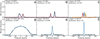 |
Fig. 1 Broadening functions of the targets that showed significant evidence being spectroscopic multiples, i.e., showed evidence of two lines (GJ 3861 and GJ 9552), or three lines (GJ 3729). We additionally show GJ 3789, and G 240-45 which do not show a double line profile in the HPF broadening functions, but are known binary systems with close (<1.7″) companions (Beuzit et al. 2004; El-Badry et al. 2021). Finally, we also show the broadening function of 2MASS J10534129+5253040, which has a high Gaia DR3 RUWE value of 2.4, which we thus assume to be a close visual binary. The blue curves show a best-fit Gaussian to the primary (i.e. brightest) peak, the red curve shows the secondary peak (if any), and the yellow peak highlights a fit to a tertiary peak (if any). The GJ 3789 broadening function is multiplied by a factor of 10 in the y-axis for enhanced readability. |
3.5 Multiplicity and broadening functions
To assess if the stars are single or spectroscopic multiples, we homogenously examined spectral-line broadening functions (Rucinski 1992) of the HPF spectra of all of the 19 Mdwarfs in the sample. The broadening function is the convolution kernel that, when applied to a template spectrum, best reproduces the observed target spectrum. The broadening functions thus represent the average photospheric absorption line profile in the spectrum. For a single star, the broadening function has a single peak. For a double star, there will generally be two peaks, unless the two radial velocities are too close to be resolved or if the secondary component is faint. Furthermore, the broadening functions allow us to obtain the rotational velocities v sin i⋆ (e.g., Tofflemire 2019), and as noted in Section 3.3, 2MASS J14333139+3417472 showed very large broadening, making it difficult to measure the v sin i⋆ through either the HPF-SpecMatch or CCF-based techniques, so we adopt the v sin i⋆ value from the broadening function analysis in this case instead.
To calculate the HPF broadening functions, we followed the methodology outlined in Stefánsson et al. (2025), which we summarize shortly here. Following Stefánsson et al. (2025), we use the saphires2 code (Tofflemire 2019), which we have adapted for HPF data. The code uses singular-value decomposition to perform the convolution inversion following Rucinski (1999). As reference template spectra we used slowly rotating inactive spectra, which were good matches to the target star from the HPF-SpecMatch analysis. By using observed data instead of synthetic spectra as templates, we bypassed the need for a model of instrumental broadening. We show the broadening functions for stars we identify as spectroscopic multiples in Figure 1, as well as the broadening functions for several close visual or spectroscopic binaries (i.e. both components falling within the HPF fiber). The broadening functions for the single-lined stars are shown in Figure C.1 in Appendix C, along with the template spectra used.
To obtain a data-driven estimate of the RV uncertainties in the broadening functions, we calculated broadening functions for four of the HPF order indices least contaminated by tellurics: order indices 5, 6, 16 and 17, covering wavelength ranges from 866–889 nm and 1027–1058 nm. This allowed us to obtain independent estimates of the RVs, and we assign the RV uncertainties as the standard deviation of the four independent RV estimates from the different HPF orders. Overall, we find that the sample contains six close visual or spectroscopic multiples (see Figure C.1), which we discuss in further detail here.
First, GJ 3789 is a known close-in binary system (ρ = 0.174″; Beuzit et al. 2004). However, due to its rapid rotation (Prot = 0.11 ± 0.01 days; see Table 1) and its long orbital period (Porb ≈ 7 yr; Beuzit et al. 2004), the resulting Keplerian velocities are small (a few km/s), and the spectral lines are highly broadened with a v sin i = 51.5 ± 4 km/s (Delfosse et al. 1998). Given that the v sin i⋆ values are much larger than the Keplerian velocities, the HPF broadening function for GJ 3789 does not exhibit clear two distinct components (see Figure 1).
Second, G 240-45 has a companion at a separation (ρ = 0.89 ± 0.07″; Lamman et al. 2020) too close for the HPF fiber to resolve, suggesting it should also appear as a spectroscopic binary. However, this target also does not show a clear double peak in its broadening function similar to GJ 3789, presumably because of small velocity separations due to a long-period orbit.
Third, Figure 1 shows that GJ 3729 exhibits three distinct peaks in its broadening functions, revealing that it is a spectroscopic triple system. As we currently have only 15 HPF observations, we lack the data necessary to robustly characterize its orbital configuration, which we leave for future work.
Fourth, GJ 9552 is a known spectroscopic binary, with an estimated separation of ρ ~ 0″.148 (Tamazian et al. 2008). This is clearly seen also in its broadening functions, which show two distinct, nearly equal-strength peaks. Previous estimates of the system’s orbital period vary, but generally suggest it is on the order of several years (Tamazian et al. 2008; Shkolnik et al. 2010; Sperauskas et al. 2019). Note, however, that the primary peak may itself consist of two components, raising the possibility that GJ 9552 is a hierarchical triple system. We acquired only two HPF observations of this target, and thus more observations are needed to confirm the existence of such a third component, as well as obtaining an accurate full orbital solution.
Fifth, for the GJ 3861 system, the distinct flux peaks between binary components allowed us to arrive at a unique orbital period and constrain the full binary orbital solution across ten HPF observations. We present this analysis in further detail in Section 5.
Sixth, we note that 2MASS J10534129+5253040 currently does not have a known stellar companion in the literature. However, we note that Gaia DR3 reports a high Gaia RUWE value of 2.4, while targets with RUWE values >1.25 are considered to likely not be a single star (Penoyre et al. 2022). The RUWE value thus suggests the presence of a binary companion with a detectable astrometric orbit over the 34-month Gaia DR3 observing baseline (Gaia Collaboration 2023). It is also over-luminous in the color-magnitude diagram (see Figure 2A) compared to the main sequence, further pointing to a likely binary companion. At the system distance of 45 pc, companions orbiting at <45 AU are well within the HPF fiber diameter of ~1.7″, which is very likely the case for this system. Despite this, the HPF broadening functions shown in Figure C do not exhibit clear evidence of double peaks. We suspect the lack of a detection of double lines in the HPF broadening functions could be due to (i) low Keplerian velocities due to a long orbital period, or (ii) a close-to face-on orbit. Nevertheless, for the reasons given above, we assign it as a ‘close visual or spectroscopic binary’ in Table 2.
We furthermore note that we cannot definitively determine whether the broad line profile of the target 2MASS J14333139+3417472 arises from the blending of lines from two rapidly rotating Mdwarfs, rather than from a single object. However, given that there is no known close companion and the Gaia RUWE value is not significantly elevated (1.08), we find no compelling evidence to suggest that this is a binary system. We therefore assume the target to be a single star.
Finally, we note that some of the targets in the sample are known wide-separated binaries: GJ 412 B (WX UMa) (Gould & Chaname 2004), GJ 860 B (Hartkopf et al. 1997), and LSPM J1024+3902E (with companion LSPM J1024+3902W; El-Badry et al. 2021). Overall, the sample altogether consists of 53% single stars, 16% well-separated binaries, and 31% HPF spectroscopic multiples (see also Table 2 and Fig. 2).
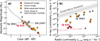 |
Fig. 2 19 radio M dwarfs studied in this work, along with the designations adopted from this work (Table 2). Targets are designated according to activity and multiplicity, and overplotted on a) a color–magnitude diagram, where we use the Gaia Catalogue of Nearby Stars (Gaia Collaboration 2021) to indicate the main sequence in gray, and b) the empirical Güdel–Benz relation (as described in Williams et al. 2014) with the 1σ spread indicated in the surrounding gray shaded region. The target G 240-45 is hereby not shown on the color–magnitude diagram, as its color is not listed in Gaia. The names of the suggested best MSPI candidates are all listed, and the systems GJ 625 and GJ 3861 – which are further discussed in Sections 4 and 5 – are highlighted in bold. |
3.6 Chromospheric activity analysis
The targets’ chromospheric activity has previously been probed through the LHα/Lbol activity indicator (Callingham et al. 2021b), the stellar flare rates seen by TESS (Pope et al. 2021), and X-ray emission. These indicators help identify whether a star’s radio emission is more likely driven by flares – which is expected in chromospherically active stars – or via MSPI, which is more expected for quiescent stars. However, these activity indicators conflict for the target GJ 450, with the LHα/Lbol < 0.09 × 10⁻⁴ indicator favoring a quiescent state (Newton et al. 2017), whereas the high TESS flare rates indicates an active state. Additionally, the target LSPM J1024+3902E neither has a published LHα/Lbol value, nor a TESS flare rate.
The HPF near-infrared spectra provide access to another activity indicator, namely the Ca II infrared triplet (Ca II IRT) (Robertson et al. 2016; Stefansson et al. 2020b). Analogous to the Ca II H & K doublet in the optical, the Ca II IRT line exhibits excess emission in active chromospheres relative to quiescent stars of similar Teff, log g, and [Fe/H] (Martin et al. 2017). As a result, the Ca II IRT has become a commonly used activity diagnostic across NIR spectroscopic programs, where traditional optical indicators such as Hα and the Ca II H & K lines are inaccessible (e.g., Schöfer et al. 2019; Lanzafame et al. 2023).
To assess the level of chromospheric activity in our targets, we examined the three Ca II IRT triples lines across the HPF observations of single-lined systems. We elected to exclude the spectroscopic multiples that show double peaks from this analysis, due to ambiguities in determining if the spectra contain emission from multiple stars. To identify ‘high’ or ‘low’ Ca II IRT emission in a model-independent manner, we follow past work (e.g., Kanodia et al. 2022) employing a reference star subtraction technique. This method involves subtracting the spectrum of an inactive reference star from the target star’s spectrum, where the reference star is matched in spectral type (or effective temperature) and artificially broadened to mimic the target’s rotational broadening. Because the reference star exhibits no Ca II IRT emission, any residual peak corresponds to intrinsic emission from the target’s chromosphere. We then calculate the equivalent width (EW) of the Ca II IRT feature and its associated uncertainty. For the calculation of the 8664 Å A Ca II IRT line, we follow Stefansson et al. (2020b) and define the EW region as the region as the vacuum wavelengths from 8664.086–8664.953 Å (highlighted in red in Figure B.1). For the EW calculation, we follow Stefansson et al. (2020b) and use the region from 8670.300–8673.190 Å as a normalization region, so the median residual of that region is unity. Hereby we do not perform any telluric correction, as these wavelength ranges are not affected by telluric contamination.
The results of the Ca II IRT line analysis at 8664 Å is shown in Figure B.1, which also lists the reference stars used. The results for the two other Ca II IRT triplet lines are the same, so we do not to show them. The figure compares the 95% highest S/N target spectra in blue, compared to the slowly rotating inactive reference star templates in black, where the template is artificially broadened to match the target v sin i⋆ values. To determine whether the targets show significant evidence of excess emission, we for each target compute the median signal-to-noise ratio of the EW of the residual emission (S/NCa II IRT,EW = EW/σEW). We classify targets with EW/σEW < 10 as showing ‘low emission’, and those with EW/σEW > 10 as showing ‘high emission’, where the dividing line was derived by visually inspecting which stars showed clear emission in the Ca II IRT residuals. We further note that two targets yield ambiguous results. For GJ 412 B, the reference spectrum does not provide a satisfactory match to the target, which is why we do not attempt to interpret the EW/σEW value in this case. We suspect that this is due to the fact that GJ 412 B (also known as WX UMa) is known to be highly magnetically active (Morin et al. 2008) and shows clear Zeeman broadening effects. We note that this does not impact the overall assessment of the activity of the star, listing it as ‘Active’ in Table 2. Additionally, 2MASS J14333139+3417472 shows significant broadening, making it difficult to detect excess emission with confidence.
Overall, we see that stars previously labeled as active – based on TESS flare rates (Pope et al. 2021) and LHα/Lbol values (Callingham et al. 2021b) – also tend to show Ca IRT emission in the HPF data. The notable exception is GJ 860 B, which lacks detectable Ca IRT emission despite exhibiting significant flare activity (0.27 ± 0.07 d−1), X-ray flux (see Figure 2), and LHα/Lbol values (LHα/Lbol = 0.64 × 10⁻⁴). Conversely, GJ 450 clearly shows Ca IRT emission, reinforcing its classification as active in agreement with TESS data, though contradicting the low LHα/Lbol < 0.09 × 10⁻⁴ value. The Ca IRT analysis also newly identifies LSPMJ1024+3902E as chromospherically active, in alignment with its rapid rotation of 2.1 ± 0.2 days as highlighted in Table 2.
Note that GJ 1151 has shown varying levels of activity across TESS sectors, as indicated by an increase in flare rate as determined more recently by Fitzmaurice et al. (2024). This suggests that we could be observing a system with a strong activity cycle, consistent with an observed polarity reversal, which occurred between 2019 and 2022 (Lehmann et al. 2024). However, as seen in Figure B.1, our Ca IRT observations do not show any significant variations in activity.
Based on all available activity indicators, we provide updated activity designation of each target in Table 2, expanding from Callingham et al. (2021b) to take into account also the target flare rates, rotation periods and Ca IRT in addition to the LHα/Lbol. We divide the sample into four stellar groups: ‘Inactive single’, ‘Active single’, ‘Active, wide-separated binary’, and ‘Close visual or spectroscopic multiple’. For the activity states, we adopt a conservative classification scheme: a target is labeled as ‘active’ if any available activity indicator shows signs of activity. Based on this definition, the most quiescent targets in the sample are GJ 625, GJ 1151, and LHS 2395.
3.7 Promising MSPI candidates in the sample
We categorize our targets based on their activity levels and multiplicity, as outlined in Table 2 (see also Sections 3.5 and 3.6). Using these classifications, we plot the targets on a color–magnitude diagram and in relation to the Güdel–Benz relation (Figure 2). The Güdel–Benz relation describes an empirical correlation between X-ray and radio luminosities observed in many active stars, typically associated with magnetic reconnection events (Benz & Güdel 1994). MSPIs are expected to result in targets that are under-luminous in X-rays relative to the Güdel-Benz relation, and although not yet fully understood, radio emission from ultra-cool dwarfs has been observed to be similarly under-luminous in X-rays (McLean et al. 2012; Williams et al. 2014). We note that long-term variability in stellar activity could also contribute to deviations from the Güdel–Benz relation, since the X-ray and radio data are generally not taken simultaneously. However, the original Güdel–Benz relation itself was also derived from nonsimultaneous observations, our comparison is in line with the original framework.
Targets most consistent with the MSPI emission scenario are expected to be under-luminous in X-rays relative to the Güdel–Benz relation, exhibit low chromospheric activity, and possess long rotation periods (Prot > 2 d) (Callingham et al. 2021b). Based on these criteria GJ 625, GJ 1151, and LHS 2395 stand out as slowly rotating and inactive stars, and thus as particularly promising MSPI candidates where the low-frequency radio detections are less likely to be due to particle acceleration in flares or through corotation breakdown. These targets furthermore show a high median RV precision (see Table 2), making them amenable to finding planets with the RV technique.
In the LOFAR radio Mdwarf sample, only two systems have known planetary companions: GJ 1151 c, and GJ 625 b. GJ 1151 was the first LOFAR uncovered radio target (Vedantham et al. 2020b) and has been extensively observed with RVs by Pope et al. (2021), Mahadevan et al. (2021), Perger et al. (2021) and Blanco-Pozo et al. (2023), showing that it hosts a likely sub-Neptune (minimum mass of m sin i = ![Mathematical equation: $\[10.62_{-1.47}^{+1.31}\]$](/articles/aa/full_html/2026/02/aa56483-25/aa56483-25-eq13.png) M⊕) on a relatively distant orbit with an orbital period P =
M⊕) on a relatively distant orbit with an orbital period P = ![Mathematical equation: $\[389.7_{-6.5}^{+5.4}\]$](/articles/aa/full_html/2026/02/aa56483-25/aa56483-25-eq14.png) d (Blanco-Pozo et al. 2023). The planet’s wide orbit likely places it beyond the Alfvénic surface – a requirement for MSPI to occur (Kavanagh et al. 2021). The available RV observations place stringent upper limits on the presence of close-in planets, ruling out the presence of ≳1M⊕ planets in close-in 1–10 day orbits. As such, it remains unclear what could have caused the LOFAR detected radio emission in the GJ 1151 system.
d (Blanco-Pozo et al. 2023). The planet’s wide orbit likely places it beyond the Alfvénic surface – a requirement for MSPI to occur (Kavanagh et al. 2021). The available RV observations place stringent upper limits on the presence of close-in planets, ruling out the presence of ≳1M⊕ planets in close-in 1–10 day orbits. As such, it remains unclear what could have caused the LOFAR detected radio emission in the GJ 1151 system.
As highlighted in Blanco-Pozo et al. (2023), GJ 1151 also shows signs of a far-out, massive companion – possibly a massive planetary companion or a brown-dwarf. Brown dwarfs are known to emit at low frequency (Vedantham et al. 2020a) radio wavelengths, so one possible scenario is that if a brown dwarf is present in the system that that could be the source of the radio emission. Recent high contrast imaging observations with JWST/NIRCAM in Cycle 3 observations have been conducted to further characterize the nature of this companion (Stefansson et al. 2024), which will be discussed in future work. Alternatively, if MSPI is operating, a close in small planet below the detection threshold of the RV measurements could also produce the observed radio signature.
In contrast, GJ 625 hosts a close-in planet with an orbital period of Porb = 14.6 days (Suárez Mascareño et al. 2017), making it a plausible candidate for MSPI. In the following section, we present an updated orbital fit for this planet, and in Section 6.2, we further explore the potential for MSPI in this system.
4 Refining the planet parameters of GJ 625 b
GJ 625 is an M2.5V-type star (see Table 1) located at a distance of 6.5 pc from Earth (Alonso-Floriano et al. 2015). As outlined above, it is a promising candidate for MSPI: it is under-luminous in X-rays relative to the Güdel–Benz relation, its activity indicators suggest minimal chromospheric activity, and it is slowly rotating. The radio emission is therefore less likely to be caused by particle acceleration in flares or through corotation breakdown, and it is amenable to precise RV observations. This target furthermore stands out in the LOFAR M dwarf radio sample, as it is the only target with a confirmed planet in a close-in orbit. The close-in orbit is key for driving MSPI, as such interactions only occur when the planet resides within the Alfvén surface.
GJ 625’s planetary companion was originally detected by Suárez Mascareño et al. (2017) using 151 HARPS-N observations over the span of 3.5 years, revealing a likely super-Earth with a minimum mass of Mp sin i = 2.82 ± 0.51M⊕ at the inner edge of the habitable zone with an orbital period of Porb = ![Mathematical equation: $\[14.628_{-0.013}^{+0.012}\]$](/articles/aa/full_html/2026/02/aa56483-25/aa56483-25-eq15.png) days. To refine the planet’s orbital parameters, we obtained additional RV measurements using the NEID spectrograph and incorporated both the original 151 HARPS-N RVs from Suárez Mascareño et al. (2017) and 49 additional HARPSN data retrieved from the TNG archive3. We also include publicly available RV measurements from the CARMENES (Ribas et al. 2023) and HIRES (Rosenthal et al. 2021) spectrographs, which respectively adds 33 and 53 new RV points. In total, this yields 140 new RV data points that have not been previously analyzed. Details of the RV extraction process are provided in Section 2.
days. To refine the planet’s orbital parameters, we obtained additional RV measurements using the NEID spectrograph and incorporated both the original 151 HARPS-N RVs from Suárez Mascareño et al. (2017) and 49 additional HARPSN data retrieved from the TNG archive3. We also include publicly available RV measurements from the CARMENES (Ribas et al. 2023) and HIRES (Rosenthal et al. 2021) spectrographs, which respectively adds 33 and 53 new RV points. In total, this yields 140 new RV data points that have not been previously analyzed. Details of the RV extraction process are provided in Section 2.
To search for and identify significant periodic signals in the expanded dataset, we used the RVSearch package (Rosenthal et al. 2021), which can generate periodograms accounting for eccentric Keplerian orbits and zero-point offsets between various datasets. The resulting periodograms of the data are shown in Figure 3, where the Bayesian Information Criterion (BIC) is used for model comparison. The BIC is calculated from the maximum likelihood (![Mathematical equation: $\[\hat{L}\]$](/articles/aa/full_html/2026/02/aa56483-25/aa56483-25-eq16.png) ) of the model as BIC = k ln(n) − 2 ln(
) of the model as BIC = k ln(n) − 2 ln(![Mathematical equation: $\[\hat{L}\]$](/articles/aa/full_html/2026/02/aa56483-25/aa56483-25-eq17.png) ), where k is the number of free parameters and n is the number of data points. We adopt a detection threshold according to an empirical False Alarm Probability (FAP) threshold of 0.1%. Figure 3 shows a comparison between a one-planet and a zero-planet model. A significant signal with ΔBIC ~ 55 is clearly seen at 14.6 days, which does not correspond to the stellar rotation period reported in Table 1. A comparison between the one-planet and two-planet models revealed no sign of other significant signals.
), where k is the number of free parameters and n is the number of data points. We adopt a detection threshold according to an empirical False Alarm Probability (FAP) threshold of 0.1%. Figure 3 shows a comparison between a one-planet and a zero-planet model. A significant signal with ΔBIC ~ 55 is clearly seen at 14.6 days, which does not correspond to the stellar rotation period reported in Table 1. A comparison between the one-planet and two-planet models revealed no sign of other significant signals.
To refine the orbital parameters of the 14.6-day signal, we performed a Keplerian fit to the RV data using the radvel package, an MCMC-based RV orbit fitting code (Fulton et al. 2018). Initial parameter estimates were taken from the results of RVsearch. For the radvel MCMC analysis we used 50 walkers, running for a total of 880 000 steps. We assessed convergence through visual inspection of the chains, where the first 200 000 steps were discarded as burn-in. The chains were deemed well-mixed, supported by a Gelman–Rubin statistic within 1% of unity, and >40 independent samples.
We show the orbital fit for the one-planet model in Figure 4, with the updated planetary parameters listed in Table 3. While the revised parameters remain consistent with those reported by Suárez Mascareño et al. (2017), the uncertainty in the orbital period has been reduced by a factor of three – from Porb = ![Mathematical equation: $\[14.628_{-0.013}^{+0.012}\]$](/articles/aa/full_html/2026/02/aa56483-25/aa56483-25-eq18.png) to Porb = 14.6288 ± 0.0027. This improvement in precision is particularly valuable for enabling future phase-resolved radio observations of upcoming radio data (see also Section 6.2).
to Porb = 14.6288 ± 0.0027. This improvement in precision is particularly valuable for enabling future phase-resolved radio observations of upcoming radio data (see also Section 6.2).
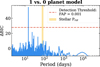 |
Fig. 3 ΔBIC periodograms of GJ 625, for the 1-planet vs. 0-planet model. The orange horizontal line shows our adopted False Alarm Probability (FAP) detection threshold of 0.1%, showing that the 14.6 d signal is significantly detected at ΔBIC ~ 55. The stellar rotation period (Prot = 80 ± 8 d) is indicated in yellow. |
5 Spectroscopic multiple: Characterization of GJ 3861
As highlighted in the broadening function of GJ 3861 (Figure 1), the HPF spectra reveal a clear set of two lines. This motivated us to obtain spectra to characterize the system in further detail. In total, we obtained 10 observations, with a median S/N of 255 at 1 μm. We extracted RVs for each BF for both the primary and secondary peaks, and as the primary and secondary peaks have clearly distinct flux ratios and heights, there is no confusion on which is the primary or the secondary peak in any of our observations. The resulting RVs for the primary and secondary peaks are listed in Table A.2 in the Appendix.
We used the method presented in Wilson (1941) to measure the mass ratio (q = M2/M1) of GJ 3861 via orthogonal distance regression of the primary velocity as a function of the secondary velocity. We implemented the orthogonal distance regression using the scipy.odr package. Figure 5 shows the ‘Wilson plot’ of the GJ 3861 system, yielding a mass ratio of q = 0.767 ± 0.002, and a velocity offset of γ = −15.092 ± 0.029 km/s.
To model the RVs using a two-component Keplerian model, we broadly follow the methodology outlined in Fernandez et al. (2017) and Skinner et al. (2018). First, we evaluated and tested different orbital periods by generating Keplerian periodograms with RVSearch. Figure 6a shows the periodogram of the primary star in GJ 3861 system (the periodogram of the secondary star looks similar), where 14.48 days shows the highest peak. We interpret this as the orbital period of the system. We further follow to calculate a ‘velocity coverage’ parameter vcov from Fernandez et al. (2017) and Skinner et al. (2018), which is given
![Mathematical equation: $\[\begin{aligned}v_{\text {cov }}=\frac{N}{N-1}\left(1-\frac{1}{\left(v_{\max }-v_{\min }\right)^2} \sum_{i=1}^N\left(v_{i+1}-v_i\right)^2\right),\end{aligned}\]$](/articles/aa/full_html/2026/02/aa56483-25/aa56483-25-eq19.png) (1)
(1)
where N is the number of observations, and vmax and vmin are the maximum and minimum RV values. As noted by Fernandez et al. (2017), the summation in Equation (1) assumes the RVs are sorted and that the mean RV has been subtracted. This parameter quantifies how much of the full RV extent the observations have covered, where Skinner et al. (2018) and Fernandez et al. (2017) found that systems with at least eight observations and vcov > 80% were sufficient to provide good enough sampling of a binary orbit to be able to accurately constrain the binary orbital properties. Using Equation (1), we estimate vcov = 95%, for GJ 3861, suggesting that we have sufficient velocity coverage to accurately constrain the binary orbital properties.
Next, we performed a Keplerian fit to the primary and secondary RVs, where the radial velocities of the primary (v1) and the secondary (v2) are
![Mathematical equation: $\[v_1=K(\cos (\nu+\omega)+e ~\cos (\omega))+\gamma,\]$](/articles/aa/full_html/2026/02/aa56483-25/aa56483-25-eq20.png) (2)
(2)
![Mathematical equation: $\[v_2=-\frac{K}{q}(\cos (\nu+\omega)+e ~\cos (\omega))+\gamma,\]$](/articles/aa/full_html/2026/02/aa56483-25/aa56483-25-eq21.png) (3)
(3)
where v is the true anomaly, which is a function of the eccentricity e, the orbital period P, and time of periastron tp, ω is the longitude of periastron, K is the RV semi-amplitude of the primary star, and γ is the RV offset of the system. In total, the set of orbital parameters we fit for are K, e, ω, tp, P and γ.
Placing an informative prior on the period (normal prior with a median of 14.86154 days and a standard deviation of 0.1 day) from the periodogram analysis, we performed a further optimization in finding a best-fit using the differential-evolution algorithm implemented in PyDE (Parviainen 2016). From this best-fit solution we initialized 100 MCMC walkers around the best-fit solution using the emcee (Foreman-Mackey et al. 2013) code, where we ran the chains for 50 000 steps, removing the first 2000 steps as burn-in. We assessed convergence by visually inspecting the chains, and verified that the Gelman-Rubin statistic is within 1% of unity, and that we have sampled at least 50 independent samples using the autocorrelation timescale feature in emcee. We therefore consider the chains well-mixed. The code we used to implement the Keplerian fit is available on GitHub4.
Figure 6b shows the RVs of GJ 3861 system along with the best-fit model, and Table 4 summarizes the priors and posteriors from the fit. From this, we see that the fit suggests a q = ![Mathematical equation: $\[0.7663_{-0.0018}^{+0.0020}\]$](/articles/aa/full_html/2026/02/aa56483-25/aa56483-25-eq22.png) , and γ =
, and γ = ![Mathematical equation: $\[-15.091_{-0.021}^{+0.019}\]$](/articles/aa/full_html/2026/02/aa56483-25/aa56483-25-eq23.png) km/s, in good agreement with the values from the Wilson plot analysis in Figure 5 which suggested q = 0.767 ± 0.002, and γ = −15.092 ± 0.029 km/s.
km/s, in good agreement with the values from the Wilson plot analysis in Figure 5 which suggested q = 0.767 ± 0.002, and γ = −15.092 ± 0.029 km/s.
Additionally, we tested models corresponding to the 1-day aliases of the 14.48 day period, corresponding to 1.07 days and 0.94 days (see Figure 6a). The 1.07 day and 0.94 day fits have much larger residuals of a few km/s and further suggest a mass ratio of q = 0.6645 ± 0.0007, and q = 0.9136 ± 0.001, respectively, both of which are inconsistent with the mass ratio derived from the Wilson plot of q = 0.767 ± 0.002. Therefore, we conclude that 14.48 days is the orbital period of the system, as listed in Table 4.
We further note that we tried both circular and eccentric fits for the GJ 3861 RV data. The circular fit resulted in significantly higher residuals at the ~2.5 km/s level – much higher than the uncertainties in the measurements – while the eccentric fit yielded residuals consistent with the scatter from the uncertainties resulting in a ΔBIC = 169 in favor of the eccentric model. We therefore adopt the eccentric model parameters, which are listed in Table 4.
Finally, we note that the RoboAO survey (Lamman et al. 2020) observed GJ 3861, which did not detect any signs of companions with Δmag < 4 from 0.45″–1.6″, and any companions with Δmag < 5 from 1.2″–1.6″. A non-detection of other companions in RoboAO is compatible with the short-period orbit we determine, which would suggest an orbit with a projected orbital separation of fractions of an arcsecond, well below the sensitivity of RoboAO.
The relatively short orbital period suggests that the system may resemble RS Canum Venaticorum (RS CVn) type binaries. We discuss this further in Section 6.3.
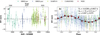 |
Fig. 4 RV observations of GJ 625. (A) RV time series of all available data of GJ 625, color-coded by spectrograph. (B) Phase folded RV data of GJ 625 phase-folded on the best-fit period of our model of 14.6288 days. The color coding is the same as in the plot on the left. Binned RV points are overplotted in red. The best-fit Keplerian model is shown in black. |
Best-fit posterior parameters for GJ 625 b.
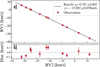 |
Fig. 5 a) Wilson plot of GJ 3861’s RVs, showing the primary RV (RV1) as a function of the secondary RV (RV2). The best-fit line (red line) suggests a mass ratio of q = 0.767 ± 0.002, and a velocity offset of γ = −15.092 ± 0.029 km/s. b) Perpendicular distance residuals to the best-fit line shown in a). |
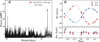 |
Fig. 6 a) Periodogram of the primary star RVs of GJ 3861. The highest peak corresponding to a period of 14.855 days is highlighted with the red dot. The 1-day aliases of the best-fit period are highlighted with the red dashed lines. b) HPF RVs of the GJ 3861 binary system. Red and blue points show the RVs of the primary and secondary, respectively. The best-fit model is shown with the red and blue curves for the primary and secondary, respectively. c) Residuals from the best-fit. RV error bars are shown with the best-fit jitter values applied in quadrature. |
GJ 3861 best-fit posteriors.
6 Discussion
6.1 Stellar inclination distribution
In Section 3, we used the values found for R⋆, Prot and v sin i⋆ to derive the stellar inclinations (i⋆) of our targets. We show the corresponding cos i⋆ values in Figure 7. The stellar inclination is a key characteristic in understanding the sample of radio-emitting Mdwarfs, as Kavanagh & Vedantham (2023) have shown that the geometry of the stellar magnetic field and planetary orbit determine the likelihood of detecting radio signatures of MSPIs. Their results suggest that if all magnetic obliquities are equally likely, blind radio surveys like V-LoTSS are more likely to observe face-on systems, where the planet orbits along the plane of the sky and the stellar rotation is observed pole-on.
Figure 7, shows no obvious bias to pole-on inclinations. However, as highlighted in Figure 7, the sample with measured stellar inclinations is solely composed of active, relatively rapidly rotating targets. Therefore, the radio emission from these targets are more likely to be associated with chromospheric activity processes or from rapid rotation, rather than needing to invoke a planetary companion to drive the observed emission. Rapid rotation can also induce ECMI, which results in strongly beamed radio emission, and thus observations of this are also expected to depend on the stellar inclination (e.g., Bloot et al. 2024). In contrast, radio emission driven by particle acceleration flares tends to be isotropic, and thus the impact of system geometry may be less pronounced.
To further quantify whether the observed inclinations show any form of clustering – i.e., inconsistent with an isotropic distribution (uniform in cos i⋆) – we performed a modified Anderson–Darling (AD) test. The AD statistic (Anderson & Darling 1952) is similar to the widely used Kolmogorov-Smirnov statistic (Feigelson & Babu 2012), but more robustly accounts for sensitivity to distribution edge effects. We broadly follow the approach of Ilin & Poppenhaeger (2022) and Ilin et al. (2024), who applied the AD test to assess clustering in stellar spin orientations. We refer the reader to the details presented in Ilin & Poppenhaeger (2022) and Ilin et al. (2024), but summarize our methodology briefly here.
We assess consistency with an isotropic distribution by comparing the AD statistic computed from our observed data (![Mathematical equation: $\[A_{\text {obs}}^{2}\]$](/articles/aa/full_html/2026/02/aa56483-25/aa56483-25-eq33.png) ) to a reference distribution of A2 values expected under the null hypothesis of isotropically distributed stellar inclinations. This reference distribution is generated by calculating A2 for 100 000 synthetic datasets, each consisting of eight cos i⋆ values randomly drawn from a uniform distribution over [0, 1]. Unlike Ilin & Poppenhaeger (2022) and Ilin et al. (2024), where measurement uncertainties were negligible, we account for the significant uncertainties in our sample. Instead of computing a single
) to a reference distribution of A2 values expected under the null hypothesis of isotropically distributed stellar inclinations. This reference distribution is generated by calculating A2 for 100 000 synthetic datasets, each consisting of eight cos i⋆ values randomly drawn from a uniform distribution over [0, 1]. Unlike Ilin & Poppenhaeger (2022) and Ilin et al. (2024), where measurement uncertainties were negligible, we account for the significant uncertainties in our sample. Instead of computing a single ![Mathematical equation: $\[A_{\text {obs}}^{2}\]$](/articles/aa/full_html/2026/02/aa56483-25/aa56483-25-eq34.png) , we generate 100 000
, we generate 100 000 ![Mathematical equation: $\[A_{\text {obs}}^{2}\]$](/articles/aa/full_html/2026/02/aa56483-25/aa56483-25-eq35.png) values, by sampling from the full posterior distributions of each target’s cos i⋆ values. We find that 96% of our posterior-based
values, by sampling from the full posterior distributions of each target’s cos i⋆ values. We find that 96% of our posterior-based ![Mathematical equation: $\[A_{\text {obs}}^{2}\]$](/articles/aa/full_html/2026/02/aa56483-25/aa56483-25-eq36.png) values exceed the critical p-value (p > 0.05), indicating that the null hypothesis of an isotropic distribution cannot be rejected.
values exceed the critical p-value (p > 0.05), indicating that the null hypothesis of an isotropic distribution cannot be rejected.
Interestingly, two of the stars in the sample, AD Leo and GJ 860 B, are observed to have close to pole-on configurations, with inclinations of ![Mathematical equation: $\[17.5_{-4.4}^{+4.0}\]$](/articles/aa/full_html/2026/02/aa56483-25/aa56483-25-eq37.png) and
and ![Mathematical equation: $\[3.5_{-1.3}^{+1.1}\]$](/articles/aa/full_html/2026/02/aa56483-25/aa56483-25-eq38.png) , respectively. Further, both stars are bright nearby stars, that show high median RV precisions, making them amenable to ground-based RV observations. However, as the stars are known to be highly active, even in the case of detection of close-in planets, this could complicate attributing any possible radio emission as being due to MSPIs. We note that AD Leo has had claims of a planet detected at the rotation period of the star at 2.24 days (Tuomi et al. 2018), but this claim has been disputed, as that signal shows clear signatures of being correlated with stellar activity indicators, with the most likely explanation being that the RV variations are due to stellar activity (Carleo et al. 2020; Robertson et al. 2020).
, respectively. Further, both stars are bright nearby stars, that show high median RV precisions, making them amenable to ground-based RV observations. However, as the stars are known to be highly active, even in the case of detection of close-in planets, this could complicate attributing any possible radio emission as being due to MSPIs. We note that AD Leo has had claims of a planet detected at the rotation period of the star at 2.24 days (Tuomi et al. 2018), but this claim has been disputed, as that signal shows clear signatures of being correlated with stellar activity indicators, with the most likely explanation being that the RV variations are due to stellar activity (Carleo et al. 2020; Robertson et al. 2020).
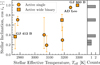 |
Fig. 7 Stellar inclinations (cos i⋆) of the subsample where we have v sin i⋆, R⋆, and Prot measurements. Left shows the cos i⋆ over the stellar effective temperature. Right shows a histogram of the cos i⋆ values. The distribution of stellar inclinations is indistinguishable from an isotropic distribution. |
6.2 Prospects for magnetic star-planet interactions on GJ 625
In Section 4, we refined the orbital parameters of GJ 625 b, deriving a period of P = 14.6288 ± 0.0027 days and a time of conjunction Tc = 2457302.9 ± 0.4. Based on this updated ephemeris, we estimate that the LOFAR radio detection reported by Callingham et al. (2021b) (2014-05-26) occurred at an orbital phase of −0.10 ± 0.06. Since that initial detection, GJ 625 has been the subject of continued LOFAR monitoring, being coincidentally located in a LoTSS deep field (ELAIS-N1; Oliver et al. 2000; Sabater et al. 2021). In total, this target has been observed in at least 21 independent LOFAR pointings over two years. The refined orbital solutions presented here facilitate a detailed phase-resolved analysis of these LOFAR observations, which will be discussed in future work.
Such an analysis is motivated by theoretical expectations that MSPI-induced radio emission is modulated by orbital phase, as the emission beam sweeps past the observer when the system’s geometry aligns favorably (Kavanagh & Vedantham 2023). In the Jupiter–Io system, for instance, radio emission is strongest near orbital quadrature (phases ±0.25). In the YZ Ceti system, bursts were detected closer to phases ±0.15 (Pineda & Villadsen 2023).
Before such a phase analysis can be meaningfully interpreted, we must assess whether conditions in the GJ 625 system are favorable for MSPI to occur. The prospects for MSPI depend primarily on the magnetic field strength at the stellar surface, and the mass-loss rate of the stellar wind. These quantities regulate the size of the Alfvén surface (Kavanagh et al. 2021), which the planet must orbit inside for MSPI to occur.
While the magnetic fields of M dwarfs manifest at both small and large spatial scales (Kochukhov 2021), the global stellar wind conditions are predominantly determined by the large-scale magnetic features on the stellar surface (Jardine et al. 2017). This ‘large-scale’ magnetic field can be mapped using the Zeeman-Doppler imaging method (ZDI; see Kochukhov 2021). However, this method has yet to be applied to GJ 625. Nevertheless, the average total magnetic field strength ⟨B⟩, which includes contributions from both the small and large-scale field, can provide a constraint on the average large-scale field strength ⟨BV⟩. Slowly rotating M dwarfs such as GJ 625 generally show that ⟨BV⟩ = 6–65% of ⟨B⟩ (Klein et al. 2021; Cristofari et al. 2023; Lehmann et al. 2024), and Reiners et al. (2022) measured a value of ⟨B⟩ = 290 G for GJ 625. Therefore, we estimate that ⟨BV⟩ ranges from 17-189 G for GJ 625.
The stellar winds of M dwarfs such as GJ 625 are tenuous, making them difficult to measure (Wood et al. 2021). However, Bloot et al. (2025) recently presented a new method for estimating upper limits for the mass-loss rates of main-sequence star with a coronal driven wind (i.e. FGKM types) based on their detection at radio wavelengths. This method relies on an estimate for ⟨BV⟩, and assumes the detected radio emission is produced by the electron cyclotron maser instability. Bloot et al. (2025) applied their method to the 19 radio-emitting M dwarfs presented by Callingham et al. (2021b), one of which being GJ 625. However, Bloot et al. (2025) estimated values of ⟨BV⟩ = 150 to 1500 G for GJ 625 based on its mass. Given that our estimate of 17 to 189 G is based on the direct measurement of the magnetic field of GJ 625 by Reiners et al. (2022), we opt to use these values instead. This range is also in closer agreement with the values measured for slowly rotating M dwarfs by Lehmann et al. (2024). Following the same method as Bloot et al. (2025)5, we estimate an upper limit for the mass-loss rate of GJ 625 of 0.68 to 25 ![Mathematical equation: $\[\dot{M}_{\odot}\]$](/articles/aa/full_html/2026/02/aa56483-25/aa56483-25-eq39.png) for our adopted range of ⟨BV⟩, where
for our adopted range of ⟨BV⟩, where ![Mathematical equation: $\[\dot{M}_{\odot}\]$](/articles/aa/full_html/2026/02/aa56483-25/aa56483-25-eq40.png) = 2 × 10⁻¹⁴ M⊙ yr−1 (Cohen 2011).
= 2 × 10⁻¹⁴ M⊙ yr−1 (Cohen 2011).
With the large-scale magnetic field strength and wind mass-loss rate of GJ 625 estimated, we now follow the same methodology as Fitzmaurice et al. (2024) to determine if GJ 625 b orbits sub-Alfvénically. For a planet to orbit inside the Alfvén surface, the Alfvénic Mach number MA of the wind at its orbit,
![Mathematical equation: $\[M_A=\frac{\Delta u}{u_A},\]$](/articles/aa/full_html/2026/02/aa56483-25/aa56483-25-eq41.png) (4)
(4)
must be less than unity (Saur et al. 2013). Here, Δu is the relative velocity between the stellar wind and the planet, and uA is the Alfvén velocity of the wind,
![Mathematical equation: $\[u_A=\frac{B}{\sqrt{4 \pi \rho}},\]$](/articles/aa/full_html/2026/02/aa56483-25/aa56483-25-eq42.png) (5)
(5)
where B is the wind magnetic field strength, and ρ is the wind density, which relates to the mass-loss rate ![Mathematical equation: $\[\dot{M}\]$](/articles/aa/full_html/2026/02/aa56483-25/aa56483-25-eq43.png) and velocity u of the stellar wind at the planet’s orbital distance a,
and velocity u of the stellar wind at the planet’s orbital distance a,
![Mathematical equation: $\[\dot{M}=4 \pi a^2 \rho u.\]$](/articles/aa/full_html/2026/02/aa56483-25/aa56483-25-eq44.png) (6)
(6)
Assuming an open magnetic field geometry for the wind at the orbit of the planet, which is likely given the long rotation period of GJ 625 (see Fitzmaurice et al. 2024), the Alfvénic Mach number can be expressed as
![Mathematical equation: $\[M_A=\frac{\Delta u}{\left\langle B_V\right\rangle}\left(\frac{a}{R_{\star}}\right)^2 \sqrt{\frac{\dot{M}}{a^2 u}}.\]$](/articles/aa/full_html/2026/02/aa56483-25/aa56483-25-eq45.png) (7)
(7)
Equation (7) illustrates how MSPI is more likely for systems with strong magnetic fields and low mass-loss rates. If ![Mathematical equation: $\[\dot{M}\]$](/articles/aa/full_html/2026/02/aa56483-25/aa56483-25-eq46.png) is an upper limit, then so too is the value of MA.
is an upper limit, then so too is the value of MA.
In Figure 8, we show the upper limit of the Mach number computed via Equation (7) over the range estimated for ⟨BV⟩ and the corresponding upper limits for ![Mathematical equation: $\[\dot{M}\]$](/articles/aa/full_html/2026/02/aa56483-25/aa56483-25-eq47.png) . We find that the maximum Mach number is less than unity for ⟨BV⟩ ≳ 20 G. This implies that MSPIs are likely for the system, as our estimated lower limit for ⟨BV⟩ is 17 G. Additionally, our mass-loss rate estimates are upper limits, so MSPIs could still occur if ⟨BV⟩ < 20 G provided the wind mass-loss rate is sufficiently low.
. We find that the maximum Mach number is less than unity for ⟨BV⟩ ≳ 20 G. This implies that MSPIs are likely for the system, as our estimated lower limit for ⟨BV⟩ is 17 G. Additionally, our mass-loss rate estimates are upper limits, so MSPIs could still occur if ⟨BV⟩ < 20 G provided the wind mass-loss rate is sufficiently low.
While these results are promising, it is worth comparing them to a system where the sub-Alfvénic nature of a planet has been assessed in more detail using a magnetic field map derived from ZDI in combination with 3D MHD stellar wind modeling. Proxima Centauri (Prox Cen) is a good choice for this. First, its comparable rotation period implies a similar large-scale magnetic field strength for GJ 625 (Vidotto et al. 2014). Second, Kavanagh et al. (2021) developed 3D MHD models for the stellar wind of Prox Cen based on its magnetic field map derived by Klein et al. (2021).
The mass-loss rate for Prox Cen is < 0.2 ![Mathematical equation: $\[\dot{M}_{\odot}\]$](/articles/aa/full_html/2026/02/aa56483-25/aa56483-25-eq48.png) (with
(with ![Mathematical equation: $\[\dot{M}_{\odot}\]$](/articles/aa/full_html/2026/02/aa56483-25/aa56483-25-eq49.png) = 2 × 10⁻¹⁴ M⊙ yr−1) (Wood et al. 2001), and its average large-scale magnetic field strength is 200 G (Klein et al. 2021). Following the same methodology as described above for GJ 625, these values give a maximum Alfvénic Mach number of 0.16 at the orbit of Prox Cen b6, which implies a sub-Alfvénic nature for planet b. However, the 3D MHD models presented by Kavanagh et al. (2021) indicate that planet b orbits outside the Alfvén surface. This discrepancy is likely due to a number of factors. For instance, the 3D MHD models from Kavanagh et al. (2021) account for the local variations in the surface magnetic field strength encapsulated by the ZDI map. Additionally, the driving mechanism of the wind in the MHD models is Alfvén waves, as opposed to the isothermal prescription adopted in the code developed by Kavanagh & Vidotto (2020). This demonstrates that while our results show promise for establishing MSPI in GJ 625, ZDI coupled to 3D magnetohydrodynamic simulations of the stellar wind outflow are needed to assess this scenario further.
= 2 × 10⁻¹⁴ M⊙ yr−1) (Wood et al. 2001), and its average large-scale magnetic field strength is 200 G (Klein et al. 2021). Following the same methodology as described above for GJ 625, these values give a maximum Alfvénic Mach number of 0.16 at the orbit of Prox Cen b6, which implies a sub-Alfvénic nature for planet b. However, the 3D MHD models presented by Kavanagh et al. (2021) indicate that planet b orbits outside the Alfvén surface. This discrepancy is likely due to a number of factors. For instance, the 3D MHD models from Kavanagh et al. (2021) account for the local variations in the surface magnetic field strength encapsulated by the ZDI map. Additionally, the driving mechanism of the wind in the MHD models is Alfvén waves, as opposed to the isothermal prescription adopted in the code developed by Kavanagh & Vidotto (2020). This demonstrates that while our results show promise for establishing MSPI in GJ 625, ZDI coupled to 3D magnetohydrodynamic simulations of the stellar wind outflow are needed to assess this scenario further.
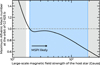 |
Fig. 8 Upper limit for the Alfvénic Mach number of the stellar wind at the orbit of GJ 625 b as a function of the average large-scale surface magnetic field strength of the host star. The gray shaded regions show where the field strength is outside the likely estimate of the magnetic field of the star from 17 to 189 G, estimated from empirical relationships. For average field strengths ≳20 G, we estimate that the planet must orbit inside the Alfvén surface, corresponding to a Mach number <1 (indicated by the dashed horizontal line). In this region (highlighted in blue), magnetic star-planet interactions can occur. However, 3D MHD simulations are needed to assess these prospects further. |
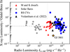 |
Fig. 9 Deviation of targets from the Güdel–Benz relation (Williams et al. 2014). The targets originally used to define this relation are shown in red, gray and blue. Coherently emitting, active targets detected with LOFAR – shown as black triangles and primarily consisting of RS CVn systems – scatter around the Güdel–Benz relation with a comparable spread (Vedantham et al. 2022). Our system, GJ 3861, is also indicated. |
6.3 GJ 3861: A possible RS CVn-like system
Our sample contains six close visual or spectroscopic multiples. In some of these, the coherent radio emission may be caused by particle acceleration in flares, as suggested by their relatively high chromospheric activity indicators. Alternatively, if the binaries are at a close-in orbit, the magnetospheric interactions between the two stars might be responsible instead. A notable target in this subsample is target GJ 9552 (CR Dra), which is located in a LoTSS deep field (specifically the ELAIS-N1 field; Oliver et al. 2000; Sabater et al. 2021). The target thus obtained numerous radio observations, allowing for a detailed analysis of its radio properties (Callingham et al. 2021a). This analysis suggests that ECMI is the most likely emission mechanism, where the instability could be driven by a breakdown in corotation.
Close-separated binaries may fall into the category of RS Canum Venaticorum (RS CVn) binaries. These systems are short-period binaries with orbital periods of ~1–30 days, typically comprising two late-type stars (F, G or K) (Hall 1976). Due to tidal locking, these systems are rapidly rotating and exhibit enhanced magnetic activity, manifesting in chromospheric emission, elevated X-ray luminosity, and significant photometric variability (e.g., Walter et al. 1978; Arévalo & Lázaro 1999; Martínez et al. 2022). Several RS CVn binaries have been observed to produce bright, coherent radio emission at LOFAR frequencies (Toet et al. 2021; Callingham et al. 2023), similar to the Mdwarf radio sample. Interestingly, although we note that the radio and X-ray observations were generally not taken simultaneously, the radio emission from these systems appears to follow the Güdel–Benz relation (See Figure 9; adapted from Vedantham et al. 2022). This behavior is unexpected for highly circularly polarized radio emission, which is typically not associated with coronal heating processes generally understood to underpin the Güdel–Benz relation. The emission mechanisms operating in these systems remain uncertain, with ECMI, plasma emission, and gyrosynchrotron emission all remaining viable interpretations (Vedantham et al. 2022).
One of the binaries in our sample, GJ 3789 (DG CVn), composed of two M4Ve-type stars, has previously been classified as an RS CVn-like system (Toet et al. 2021; Vedantham et al. 2022). However, its estimated orbital period of approximately 7 years (Beuzit et al. 2004) is significantly longer than the typical 1–30 day range for RS CVn binaries, calling this classification into question. The orbital periods of G 240-45, GJ 3729, and 2MASS J10534129+5253040 are furthermore unknown and the orbital period of GJ 9552 remains uncertain (Tamazian et al. 2008; Shkolnik et al. 2010; Sperauskas et al. 2019). Therefore, it is unclear if these systems can be decisively called RS CVn-like binaries.
In contrast, in Section 5, we have shown that GJ 3861 is a binary with a mass ratio of q = ![Mathematical equation: $\[0.7663_{-0.0018}^{+0.0020}\]$](/articles/aa/full_html/2026/02/aa56483-25/aa56483-25-eq50.png) , and an orbital period of P = 14.841181 ± 0.00010 d, making it the only system in the M dwarf radio sample with a confirmed short-period orbit, compatible with the RS CVn-like classification. As further shown in Figure D.1, ground-based photometry from ZTF reveals a detection of photometric modulations at periods from 12–16 days, further confirming its activity and compatibility with an RS CVn-like binary. However, GJ 3861 deviates more significantly from the Güdel–Benz relation than the other known RS CVn systems with coherent radio emission (see Figure 9), with a deviation of 2.8σ, where σ denotes the standard deviation scatter seen in the systems discussed by Vedantham et al. (2022). Even so, given the close-in active stars in a close-in orbital period we surmise that the most likely reason for the observed radio emission in the system is related to either the chromospheric activity and/or interaction of magnetospheres in the system.
, and an orbital period of P = 14.841181 ± 0.00010 d, making it the only system in the M dwarf radio sample with a confirmed short-period orbit, compatible with the RS CVn-like classification. As further shown in Figure D.1, ground-based photometry from ZTF reveals a detection of photometric modulations at periods from 12–16 days, further confirming its activity and compatibility with an RS CVn-like binary. However, GJ 3861 deviates more significantly from the Güdel–Benz relation than the other known RS CVn systems with coherent radio emission (see Figure 9), with a deviation of 2.8σ, where σ denotes the standard deviation scatter seen in the systems discussed by Vedantham et al. (2022). Even so, given the close-in active stars in a close-in orbital period we surmise that the most likely reason for the observed radio emission in the system is related to either the chromospheric activity and/or interaction of magnetospheres in the system.
We additionally note that GJ 3861 has not previously been recognized as a close-in binary system, which might have implications on previous work. One such example is the work of Bloot et al. (2025), which used LOFAR observations to characterize the stellar mass-loss rates of the LOFAR radio emitting sample discussed here, where they highlight GJ 3861 as a representative case in placing constraints on stellar mass-loss rates. Assuming a single star, for GJ 3861 they find a mass loss rate of 200–1120 ![Mathematical equation: $\[\dot{M}_{\odot}\]$](/articles/aa/full_html/2026/02/aa56483-25/aa56483-25-eq51.png) . However, as their method assumes a single stellar wind source, rather than a binary, the detected emission may arise from contribution from both stellar components. As such, although Bloot et al. (2025) place much more stringent constraints than earlier studies on the mass-loss of GJ 3861, the derived stellar mass loss rate may be overestimated due to the unaccounted contribution from the secondary.
. However, as their method assumes a single stellar wind source, rather than a binary, the detected emission may arise from contribution from both stellar components. As such, although Bloot et al. (2025) place much more stringent constraints than earlier studies on the mass-loss of GJ 3861, the derived stellar mass loss rate may be overestimated due to the unaccounted contribution from the secondary.
7 Summary and conclusions
We present the first results of a spectroscopic survey to characterize recent radio detections of radio emitting M dwarfs identified as coherent radio sources by the LOFAR Two-Metre Sky Survey. Using high-resolution NIR and red-optical spectroscopic data from the HPF and NEID spectrographs, we homogeneously derive stellar spectroscopic properties and further assess the nature of the observed radio emission. Our key findings for the sample as a whole are as follows:
Stellar properties and MSPI targets: We measure the sample’s stellar properties, including their effective temperatures (Teff), surface gravities (log g), metallicities ([Fe/H]), projected rotational velocities (v sin i⋆), rotation periods (Prot), stellar radii (R⋆), and stellar inclinations (i⋆). We find that the sample consists of 53% (10/19) single, 16% (3/19) well-separated binaries, and 31% (6/19) close visual or spectroscopic multiples. We identify three stars in the sample – GJ 625, GJ 1151, and LHS 2395 – that are chromospherically inactive and which are amenable to finding close-in planet with RVs, making them particularly favorable MSPI candidates;
Distribution of stellar inclinations: Certain models for the MSPI origin of the emission suggests that there could be an overabundance of pole-on configurations for the stellar inclinations. However, in investigating the sample of 8 stars with measured stellar inclinations, we show that by sampling from their posteriors that in 96% of the cases, the measured distribution is indistinguishable from an isotropic distribution. However, our sample of radio-bright stars with measured inclinations are dominated by active, and in some cases rapidly-rotating, stars;
Refining the orbit of GJ 625 b: GJ 625 hosts a previously confirmed close-in planet. By combining new RV data with archival measurements, we refine the planet’s orbital ephemeris by a factor of three in precision, providing an improved baseline for future phase-targeted radio monitoring. Furthermore, we estimate that the system conditions are suitable for MSPIs, given a sufficiently strong stellar magnetic field. Future Zeeman-Doppler Imaging observations to constrain the large scale stellar magnetic field are needed to further assess the MSPIs scenario;
GJ 3861 as a candidate RS CVn-like system: For the first time, we reveal GJ 3861 to be a double-lined spectroscopic binary with an orbital period of
![Mathematical equation: $\[14.841181_{-0.00010}^{+0.00011}\]$](/articles/aa/full_html/2026/02/aa56483-25/aa56483-25-eq52.png) days and a mass ratio of q =
days and a mass ratio of q = ![Mathematical equation: $\[0.7663_{-0.0018}^{+0.0020}\]$](/articles/aa/full_html/2026/02/aa56483-25/aa56483-25-eq53.png) . Its relatively short orbital period is characteristic of RS CVn systems, which have been seen to emit bright, circularly polarized radio emission.
. Its relatively short orbital period is characteristic of RS CVn systems, which have been seen to emit bright, circularly polarized radio emission.
Data availability
Tables 1 and A.1 and A.2 are available at the CDS via https://cdsarc.cds.unistra.fr/viz-bin/cat/J/A+A/706/A98. A reproduction package can be found on Zenodo under https://doi.org/10.5281/zenodo.15491027. The package includes a relatively high S/N spectrum of each target, and all used NEID and HPF spectra of GJ 3861 and GJ 625. The package also includes intermediate data products that can be used to reproduce the figures in this paper.
Acknowledgements
These results are based on observations obtained with the Habitable-zone Planet Finder Spectrograph on the HET. The HPF team acknowledges support from NSF grants AST-1006676, AST-1126413, AST-1310885, AST-1517592, AST-1310875, ATI 2009889, ATI-2009982, AST-2108512, and the NASA Astrobiology Institute (NNA09DA76A) in the pursuit of precision radial velocities in the NIR. The HPF team also acknowledges support from the Heising-Simons Foundation via grant 2017-0494. This research was conducted in part under NSF grants AST-2108493, AST-2108512, AST-2108569, and AST-2108801 in support of the HPF Guaranteed Time Observations survey. Based on observations obtained with the Hobby-Eberly Telescope (HET), which is a joint project of the University of Texas at Austin, the Pennsylvania State University, Ludwig-Maximillians-Universitaet Muenchen, and Georg-August Universitaet Goettingen. The HET is named in honor of its principal benefactors, William P. Hobby and Robert E. Eberly. We acknowledge support from NASA XRP Grant 80NSSC24K0155. We acknowledge the Texas Advanced Computing Center (TACC) at the University of Texas at Austin for providing high performance computing, visualization, and storage resources that have contributed to the results reported within this paper. We thank the Resident astronomers and Telescope Operators at the HET for the skillful execution of our observations with HPF. Data presented were obtained by the NEID spectrograph built by Penn State University and operated at the WIYN Observatory by NOIRLab, under the NN-EXPLORE partnership of the National Aeronautics and Space Administration and the National Science Foundation. The NEID archive is operated by the NASA Exoplanet Science Institute at the California Institute of Technology. We thank the NEID Queue Observers and WIYN Observing Associates for their skillful execution of our observations. Based on observations at NSF Kitt Peak National Observatory, NSF NOIRLab (NOIRLab Prop. ID 2021A-0389, PI Paul Robertson, and NOIRLab Prop. ID 2022A-452266, PI Shubham Kanodia), which is managed by the Association of Universities for Research in Astronomy (AURA) under a cooperative agreement with the U.S. National Science Foundation. The authors are honored to be permitted to conduct astronomical research on I’oligam Du’ag (Kitt Peak), a mountain with particular significance to the Tohono O’odham. Based on data from the CARMENES data archive at CAB (CSIC-INTA). The CARMENES archive is part of the Spanish Virtual Observatory project (http://svo.cab.inta-csic.es), funded by MCIN/AEI/10.13039/501100011033/ through grant PID2020-112949GB-I00. This research has made use of the Keck Observatory Archive (KOA), which is operated by the W.M. Keck Observatory and the NASA Exoplanet Science Institute (NExScI), under contract with the National Aeronautics and Space Administration. This research used the facilities of the Italian Center for Astronomical Archive (IA2) operated by INAF at the Astronomical Observatory of Trieste. This research made use of the NASA Exoplanet Archive, which is operated by the California Institute of Technology, under contract with the National Aeronautics and Space Administration under the Exoplanet Exploration Program. This work has made use of data from the European Space Agency (ESA) mission Gaia processed by the Gaia Data Processing and Analysis Consortium (DPAC). The Center for Exoplanets and Habitable Worlds and the Penn State Extraterrestrial Intelligence Center are supported by Penn State and its Eberly College of Science. R.D.K. acknowledges funding from the Dutch Research Council (NWO) for the project ‘e-MAPS’ (project number Vi.Vidi.203.093) under the NWO talent scheme VIDI. J.I.E.-R. gratefully acknowledges support from the ANID BASAL project FB210003 and from the ANID Doctorado Nacional grant 2021-21212378. C.I.C. acknowledges support by NASA Headquarters through an appointment to the NASA Postdoctoral Program at the Goddard Space Flight Center, administered by ORAU through a contract with NASA. J.R.C. acknowledges funding from the European Union via the European Research Council (ERC) grant Epaphus (project number: 101166008). The research was carried out, in part, at the Jet Propulsion Laboratory, California Institute of Technology, under a contract with the National Aeronautics and Space Administration (80NM0018D0004).
References
- Alonso-Floriano, F. J., Morales, J. C., Caballero, J. A., et al. 2015, A&A, 577, A128 [NASA ADS] [CrossRef] [EDP Sciences] [Google Scholar]
- Anderson, T. W., & Darling, D. A. 1952, Ann. Math. Statist., 23, 193 [CrossRef] [Google Scholar]
- Arévalo, M. J., & Lázaro, C. 1999, AJ, 118, 1015 [Google Scholar]
- Bailer-Jones, C. A. L., Rybizki, J., Fouesneau, M., Demleitner, M., & Andrae, R. 2021, AJ, 161, 147 [Google Scholar]
- Benz, A. O., & Güdel, M. 1994, A&A, 285, 621 [Google Scholar]
- Beuzit, J.-L., Ségransan, D., Forveille, T., et al. 2004, A&A, 425, 997 [NASA ADS] [CrossRef] [EDP Sciences] [Google Scholar]
- Bigg, E. K. 1964, Nature, 203, 1008 [NASA ADS] [CrossRef] [Google Scholar]
- Blanco-Pozo, J., Perger, M., Damasso, M., et al. 2023, A&A, 671, A50 [NASA ADS] [CrossRef] [EDP Sciences] [Google Scholar]
- Bloot, S., Callingham, J. R., Vedantham, H. K., et al. 2024, A&A, 682, A170 [NASA ADS] [CrossRef] [EDP Sciences] [Google Scholar]
- Bloot, S., Vedantham, H. K., Kavanagh, R. D., Callingham, J. R., & Pope, B. J. S. 2025, A&A, 695, A176 [NASA ADS] [CrossRef] [EDP Sciences] [Google Scholar]
- Burke, B. F., & Franklin, K. L. 1955, J. Geophys. Res., 60, 213 [NASA ADS] [CrossRef] [Google Scholar]
- Busso, G., Cacciari, C., Bellazzini, M., et al. 2022, Gaia DR3 documentation Chapter 5: Photometric data [Google Scholar]
- Callingham, J. R., Pope, B. J. S., Feinstein, A. D., et al. 2021a, A&A, 648, A13 [EDP Sciences] [Google Scholar]
- Callingham, J. R., Vedantham, H. K., Shimwell, T. W., et al. 2021b, Nat. Astron., 5, 1233 [NASA ADS] [CrossRef] [Google Scholar]
- Callingham, J. R., Shimwell, T. W., Vedantham, H. K., et al. 2023, A&A, 670, A124 [NASA ADS] [CrossRef] [EDP Sciences] [Google Scholar]
- Callingham, J. R., Pope, B. J. S., Kavanagh, R. D., et al. 2024, Nat. Astron., 8, 1359 [NASA ADS] [CrossRef] [Google Scholar]
- Carleo, I., Malavolta, L., Lanza, A. F., et al. 2020, A&A, 638, A5 [NASA ADS] [CrossRef] [EDP Sciences] [Google Scholar]
- Cauley, P. W., Shkolnik, E. L., Llama, J., & Lanza, A. F. 2019, Nat. Astron., 3, 1128 [NASA ADS] [CrossRef] [Google Scholar]
- Cohen, O. 2011, MNRAS, 417, 2592 [Google Scholar]
- Cosentino, R., Lovis, C., Pepe, F., et al. 2012, in Ground-based and Airborne Instrumentation for Astronomy IV, eds. I. S. McLean, S. K. Ramsay, & H. Takami (SPIE) [Google Scholar]
- Cristofari, P. I., Donati, J. F., Moutou, C., et al. 2023, MNRAS, 526, 5648 [NASA ADS] [CrossRef] [Google Scholar]
- Delfosse, X., Forveille, T., Perrier, C., & Mayor, M. 1998, A&A, 331, 581 [NASA ADS] [Google Scholar]
- Dulk, G. A. 1985, ARA&A, 23, 169 [Google Scholar]
- El-Badry, K., Rix, H.-W., & Heintz, T. M. 2021, MNRAS, 506, 2269 [NASA ADS] [CrossRef] [Google Scholar]
- Feigelson, E. D., & Babu, G. J. 2012, Modern Statistical Methods for Astronomy: With R Applications (Cambridge University Press) [Google Scholar]
- Fernandez, M. A., Covey, K. R., De Lee, N., et al. 2017, PASP, 129, 084201 [NASA ADS] [CrossRef] [Google Scholar]
- Fitzmaurice, E., Stefánsson, G., Kavanagh, R. D., et al. 2024, AJ, 168, 140 [Google Scholar]
- Foreman-Mackey, D., Hogg, D. W., Lang, D., & Goodman, J. 2013, PASP, 125, 306 [Google Scholar]
- Fulton, B. J., Petigura, E. A., Blunt, S., & Sinukoff, E. 2018, PASP, 130, 044504 [Google Scholar]
- Gaia Collaboration (Smart, R. L., et al.) 2021, A&A, 649, A6 [EDP Sciences] [Google Scholar]
- Gaia Collaboration (Vallenari, A., et al.) 2023, A&A, 674, A1 [NASA ADS] [CrossRef] [EDP Sciences] [Google Scholar]
- Garcia-Sage, K., Glocer, A., Drake, J. J., Gronoff, G., & Cohen, O. 2017, ApJ, 844, L13 [NASA ADS] [CrossRef] [Google Scholar]
- Gould, A., & Chaname, J. 2004, ApJS, 150, 455 [CrossRef] [Google Scholar]
- Gupta, Y., Ajithkumar, B., Kale, H. S., et al. 2017, Curr. Sci., 113, 707 [NASA ADS] [CrossRef] [Google Scholar]
- Hall, D. S. 1976, in Astrophysics and Space Science Library, 60, IAU Colloq. 29: Multiple Periodic Variable Stars, ed. W. S. Fitch, 287 [Google Scholar]
- Hartkopf, W. I., McAlister, H. A., Mason, B. D., et al. 1997, AJ, 114, 1639 [Google Scholar]
- Hess, S. L. G., & Zarka, P. 2011, A&A, 531, A29 [NASA ADS] [CrossRef] [EDP Sciences] [Google Scholar]
- Hill, G. J., Lee, H., MacQueen, P. J., et al. 2021, AJ, 162, 298 [NASA ADS] [CrossRef] [Google Scholar]
- Ilin, E., & Poppenhaeger, K. 2022, MNRAS, 513, 4579 [NASA ADS] [CrossRef] [Google Scholar]
- Ilin, E., Poppenhäger, K., Chebly, J., Ilić, N., & Alvarado-Gómez, J. D. 2024, MNRAS, 527, 3395 [Google Scholar]
- Ilin, E., Vedantham, H. K., Poppenhäger, K., et al. 2025, Nature 643, 645 [Google Scholar]
- Jardine, M., Vidotto, A. A., & See, V. 2017, MNRAS, 465, L25 [Google Scholar]
- Johnston, S., Taylor, R., Bailes, M., et al. 2008, Exp. Astron., 22, 151 [Google Scholar]
- Johnstone, C. P., & Güdel, M. 2015, A&A, 578, A129 [NASA ADS] [CrossRef] [EDP Sciences] [Google Scholar]
- Jones, S. E., Stefánsson, G., Masuda, K., et al. 2024, AJ, 168, 93 [NASA ADS] [Google Scholar]
- Kanodia, S., Mahadevan, S., Ramsey, L. W., et al. 2018, in Ground-based and Airborne Instrumentation for Astronomy VII, eds. H. Takami, C. J. Evans, & L. Simard (SPIE), 245 [Google Scholar]
- Kanodia, S., Ramsey, L. W., Maney, M., et al. 2022, ApJ, 925, 155 [NASA ADS] [CrossRef] [Google Scholar]
- Kanodia, S., Lin, A. S. J., Lubar, E., et al. 2023, AJ, 166, 105 [Google Scholar]
- Kavanagh, R. D., & Vedantham, H. K. 2023, MNRAS, 524, 6267 [NASA ADS] [CrossRef] [Google Scholar]
- Kavanagh, R. D., & Vidotto, A. A. 2020, MNRAS, 493, 1492 [Google Scholar]
- Kavanagh, R. D., Vidotto, A. A., Klein, B., et al. 2021, MNRAS, 504, 1511 [Google Scholar]
- Kavanagh, R. D., Vidotto, A. A., Vedantham, H. K., et al. 2022, MNRAS, 514, 675 [CrossRef] [Google Scholar]
- Kiman, R., Schmidt, S. J., Angus, R., et al. 2019, AJ, 157, 231 [CrossRef] [Google Scholar]
- Klein, B., Donati, J.-F., Hébrard, É. M., et al. 2021, MNRAS, 500, 1844 [Google Scholar]
- Kochukhov, O. 2021, A&A Rev., 29, 1 [Google Scholar]
- Lamman, C., Baranec, C., Berta-Thompson, Z. K., et al. 2020, AJ, 159, 139 [Google Scholar]
- Lanza, A. F. 2018, A&A, 610, A81 [NASA ADS] [CrossRef] [EDP Sciences] [Google Scholar]
- Lanzafame, A. C., Brugaletta, E., Frémat, Y., et al. 2023, A&A, 674, A30 [NASA ADS] [CrossRef] [EDP Sciences] [Google Scholar]
- Lecavelier des Etangs, A., Sirothia, S. K., Gopal-Krishna, & Zarka, P. 2013, A&A, 552, A65 [NASA ADS] [CrossRef] [EDP Sciences] [Google Scholar]
- Lehmann, L. T., Donati, J. F., Fouqué, P., et al. 2024, MNRAS, 527, 4330 [Google Scholar]
- Mahadevan, S., Ramsey, L., Bender, C., et al. 2012, in Ground-based and Airborne Instrumentation for Astronomy IV, eds. I. S. McLean, S. K. Ramsay, & H. Takami (SPIE) [Google Scholar]
- Mahadevan, S., Ramsey, L. W., Terrien, R., et al. 2014, in Ground-based and Airborne Instrumentation for Astronomy V, 9147, eds. S. K. Ramsay, I. S. McLean, & H. Takami (SPIE), 91471G [Google Scholar]
- Mahadevan, S., Stefánsson, G., Robertson, P., et al. 2021, ApJ, 919, L9 [NASA ADS] [CrossRef] [Google Scholar]
- Mann, A. W., Feiden, G. A., Gaidos, E., Boyajian, T., & Braun, K. v. 2015, ApJ, 804, 64 [CrossRef] [Google Scholar]
- Martin, J., Fuhrmeister, B., Mittag, M., et al. 2017, A&A, 605, A113 [NASA ADS] [CrossRef] [EDP Sciences] [Google Scholar]
- Martínez, C. I., Mauas, P. J. D., & Buccino, A. P. 2022, MNRAS, 512, 4835 [CrossRef] [Google Scholar]
- Masci, F. J., Laher, R. R., Rusholme, B., et al. 2019, PASP, 131, 018003 [Google Scholar]
- Masuda, K., & Winn, J. N. 2020, AJ, 159, 81 [NASA ADS] [CrossRef] [Google Scholar]
- McLean, M., Berger, E., & Reiners, A. 2012, ApJ, 746, 23 [Google Scholar]
- Morin, J., Donati, J. F., Petit, P., et al. 2008, MNRAS, 390, 567 [Google Scholar]
- Newton, E. R., Irwin, J., Charbonneau, D., et al. 2017, ApJ, 834, 85 [Google Scholar]
- Ninan, J. P., Mahadevan, S., Stefansson, G., et al. 2019, J. Astron. Telesc. Instrum. Syst., 5, 1 [CrossRef] [Google Scholar]
- Oliver, S., Rowan-Robinson, M., Alexander, D. M., et al. 2000, MNRAS, 316, 749 [Google Scholar]
- Owen, J. E., & Adams, F. C. 2014, MNRAS, 444, 3761 [Google Scholar]
- Parviainen, H. 2016, https://doi.org/10.5281/zenodo.45602 [Google Scholar]
- Penoyre, Z., Belokurov, V., & Evans, N. W. 2022, MNRAS, 513, 2437 [NASA ADS] [CrossRef] [Google Scholar]
- Pérez-Torres, M., Gómez, J. F., Ortiz, J. L., et al. 2021, A&A, 645, A77 [NASA ADS] [CrossRef] [EDP Sciences] [Google Scholar]
- Perger, M., Ribas, I., Anglada-Escudé, G., et al. 2021, A&A, 649, L12 [EDP Sciences] [Google Scholar]
- Pineda, J. S., & Villadsen, J. 2023, Nat. Astron., 7, 569 [NASA ADS] [CrossRef] [Google Scholar]
- Pope, B. J. S., Callingham, J. R., Feinstein, A. D., et al. 2021, ApJ, 919, L10 [NASA ADS] [CrossRef] [Google Scholar]
- Presa, A., Driessen, F. A., & Vidotto, A. A. 2024, MNRAS, 534, 3622 [Google Scholar]
- Quirrenbach, A., CARMENES Consortium, Amado, P. J., et al. 2020, SPIE Conf. Ser., 11447, 114473C [NASA ADS] [Google Scholar]
- Ramsey, L. W., Adams, M. T., Barnes III, T. G., et al. 1998, in Advanced Technology Optical/IR Telescopes VI, ed. L. M. Stepp (SPIE) [Google Scholar]
- Reiners, A. 2007, A&A, 467, 259 [NASA ADS] [CrossRef] [EDP Sciences] [Google Scholar]
- Reiners, A., Shulyak, D., Käpylä, P. J., et al. 2022, A&A, 662, A41 [NASA ADS] [CrossRef] [EDP Sciences] [Google Scholar]
- Ribas, I., Reiners, A., Zechmeister, M., et al. 2023, A&A, 670, A139 [NASA ADS] [CrossRef] [EDP Sciences] [Google Scholar]
- Robertson, P., Bender, C., Mahadevan, S., Roy, A., & Ramsey, L. W. 2016, ApJ, 832, 112 [CrossRef] [Google Scholar]
- Robertson, P., Anderson, T., Stefansson, G., et al. 2019, J. Astron. Telesc. Instrum. Syst., 5, 015003 [Google Scholar]
- Robertson, P., Stefansson, G., Mahadevan, S., et al. 2020, ApJ, 897, 125 [NASA ADS] [CrossRef] [Google Scholar]
- Rosenthal, L. J., Fulton, B. J., Hirsch, L. A., et al. 2021, ApJS, 255, 8 [NASA ADS] [CrossRef] [Google Scholar]
- Rubenstein, E. P., & Schaefer, B. E. 2000, ApJ, 529, 1031 [Google Scholar]
- Rucinski, S. 1999, Turkish J. Phys., 23, 271 [Google Scholar]
- Rucinski, S. M. 1992, AJ, 104, 1968 [Google Scholar]
- Sabater, J., Best, P. N., Tasse, C., et al. 2021, A&A, 648, A2 [EDP Sciences] [Google Scholar]
- Saur, J., Grambusch, T., Duling, S., Neubauer, F. M., & Simon, S. 2013, A&A, 552, A119 [NASA ADS] [CrossRef] [EDP Sciences] [Google Scholar]
- Schöfer, P., Jeffers, S. V., Reiners, A., et al. 2019, A&A, 623, A44 [Google Scholar]
- Schwab, C., Rakich, A., Gong, Q., et al. 2016, in Ground-based and Airborne Instrumentation for Astronomy VI, 9909, eds. C. J. Evans, L. Simard, & H. Takami (SPIE), 99087H [Google Scholar]
- Shetrone, M., Cornell, M., Fowler, J., et al. 2007, PASP, 119, 556–566 [Google Scholar]
- Shields, A. L., Ballard, S., & Johnson, J. A. 2016, Phys. Rep., 663, 1 [NASA ADS] [CrossRef] [Google Scholar]
- Shimwell, T. W., Tasse, C., Hardcastle, M. J., et al. 2019, A&A, 622, A1 [NASA ADS] [CrossRef] [EDP Sciences] [Google Scholar]
- Shkolnik, E. 2004, PhD thesis, University of British Columbia, Canada [Google Scholar]
- Shkolnik, E. L., Hebb, L., Liu, M. C., Reid, I. N., & Collier Cameron, A. 2010, ApJ, 716, 1522 [Google Scholar]
- Shulyak, D., Reiners, A., Wende, S., et al. 2010, A&A, 523, A37 [NASA ADS] [CrossRef] [EDP Sciences] [Google Scholar]
- Skinner, J., Covey, K. R., Bender, C. F., et al. 2018, AJ, 156, 45 [NASA ADS] [CrossRef] [Google Scholar]
- Sperauskas, J., Deveikis, V., & Tokovinin, A. 2019, A&A, 626, A31 [NASA ADS] [CrossRef] [EDP Sciences] [Google Scholar]
- Stassun, K. G., Oelkers, R. J., Pepper, J., et al. 2018, AJ, 156, 102 [Google Scholar]
- Stefansson, G., Hearty, F., Robertson, P., et al. 2016, ApJ, 833, 175 [NASA ADS] [CrossRef] [Google Scholar]
- Stefansson, G., Cañas, C., Wisniewski, J., et al. 2020a, AJ, 159, 100 [NASA ADS] [CrossRef] [Google Scholar]
- Stefansson, G., Mahadevan, S., Maney, M., et al. 2020b, AJ, 160, 192 [NASA ADS] [CrossRef] [Google Scholar]
- Stefànsson, G., Mahadevan, S., Petrovich, C., et al. 2022, ApJ, 931, L15 [NASA ADS] [CrossRef] [Google Scholar]
- Stefánsson, G., Mahadevan, S., Miguel, Y., et al. 2023, Science, 382, 1031 [CrossRef] [Google Scholar]
- Stefansson, G., Patapis, P. A., Callingham, J., et al. 2024, Resolving the Radio Riddle: Unveiling the Origins of Radio Emission in a Red Dwarf and its WideOrbit Companion, JWST Proposal. Cycle 3, ID. #5497 [Google Scholar]
- Stefánsson, G., Mahadevan, S., Winn, J. N., et al. 2025, AJ, 169, 107 [Google Scholar]
- Suárez Mascareño, A., González Hernández, J. I., Rebolo, R., et al. 2017, A&A, 605, A92 [NASA ADS] [CrossRef] [EDP Sciences] [Google Scholar]
- Tamazian, V. S., Docobo, J. A., Balega, Y. Y., et al. 2008, AJ, 136, 974 [Google Scholar]
- Toet, S. E. B., Vedantham, H. K., Callingham, J. R., et al. 2021, A&A, 654, A21 [NASA ADS] [CrossRef] [EDP Sciences] [Google Scholar]
- Tofflemire, B. M. 2019, https://zenodo.org/record/3497508 [Google Scholar]
- Treumann, R. A. 2006, A&A Rev., 13, 229 [Google Scholar]
- Trigilio, C., Biswas, A., Leto, P., et al. 2023, arXiv e-prints [arXiv:2305.00809] [Google Scholar]
- Tuomi, M., Jones, H. R. A., Barnes, J. R., et al. 2018, AJ, 155, 192 [NASA ADS] [CrossRef] [Google Scholar]
- Turner, J. D., Zarka, P., Grießmeier, J.-M., et al. 2021, A&A, 645, A59 [NASA ADS] [CrossRef] [EDP Sciences] [Google Scholar]
- van Haarlem, M. P., Wise, M. W., Gunst, A. W., et al. 2013, A&A, 556, A2 [NASA ADS] [CrossRef] [EDP Sciences] [Google Scholar]
- Vedantham, H. K., Callingham, J. R., Shimwell, T. W., et al. 2020a, ApJ, 903, L33 [Google Scholar]
- Vedantham, H. K., Callingham, J. R., Shimwell, T. W., et al. 2020b, Nat. Astron., 4, 577 [Google Scholar]
- Vedantham, H. K., Callingham, J. R., Shimwell, T. W., et al. 2022, ApJ, 926, L30 [NASA ADS] [CrossRef] [Google Scholar]
- Vidotto, A. A., Gregory, S. G., Jardine, M., et al. 2014, MNRAS, 441, 2361 [Google Scholar]
- Vogt, S. S., Allen, S. L., Bigelow, B. C., et al. 1994, in Instrumentation in Astronomy VIII, eds. D. L. Crawford, & E. R. Craine (SPIE) [Google Scholar]
- Walter, F., Charles, P., & Bowyer, S. 1978, ApJ, 225, L119 [NASA ADS] [CrossRef] [Google Scholar]
- Williams, P. K. G., Cook, B. A., & Berger, E. 2014, ApJ, 785, 9 [Google Scholar]
- Wilson, O. C. 1941, ApJ, 93, 29 [NASA ADS] [CrossRef] [Google Scholar]
- Wood, B. E., Linsky, J. L., Müller, H.-R., & Zank, G. P. 2001, ApJ, 547, L49 [NASA ADS] [CrossRef] [Google Scholar]
- Wood, B. E., Müller, H.-R., Redfield, S., et al. 2021, ApJ, 915, 37 [NASA ADS] [CrossRef] [Google Scholar]
- Zarka, P. 2018, in Handbook of Exoplanets, eds. H. J. Deeg & J. A. Belmonte, 22 [Google Scholar]
- Zechmeister, M., Reiners, A., Amado, P. J., et al. 2018, A&A, 609, A12 [NASA ADS] [CrossRef] [EDP Sciences] [Google Scholar]
The WIYN Observatory is a joint facility of the University of Wisconsin–Madison, Indiana University, NSF NOIRLab, the Pennsylvania State University, and Princeton University.
To estimate the wind velocity of Prox Cen, we use the code developed by Kavanagh & Vidotto (2020), adopting a mass and radius of 0.12 M⊙ and 0.14 R⊙ (Kavanagh et al. 2021), and coronal temperature of 2.70 MK (Johnstone & Güdel 2015). Note that we reduce the temperature from the corona to the wind by a factor of 1.36, as done by Bloot et al. (2025).
Appendix A RVs
Table A.1, and Table A.2 lists the RVs of GJ 625 and GJ 3861, respectively.
The first and last 20 GJ 625 RVs used in its orbit analysis.
GJ 3861 RVs. v1 and σ1 lists the RVs and corresponding uncertainties of the primary star, and v2 and σ2 list the rvs RVs and uncertainties of the secondary star.
Appendix B Ca IRT emission
Figure B.1 shows the Ca IRT line of all our observations (blue), with a slowly-rotating, quiescent reference star shown in black.
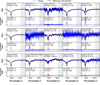 |
Fig. B.1 HPF observations of the Ca II IRT line at 8664 Å for all non-SB2 targets in the M dwarf radio sample (blue curves), compared to a single high S/N as-observed HPF spectrum of slowly rotating quiescent reference stars (black). The reference spectrum is rotationally broadened to match the observed broadening of the lines, by using the estimates of the v sin i obtained by HPF-SpecMatch. The red shaded region marks the line center, which is the emission window used to compute the Equivalent Width. The lower panels show the normalized ratio residuals (target/reference), highlighting any excess emission as a peak in the residuals. A continuum region (8670.300–8673.190 Å, gray shaded) is used to normalize the residuals to unity. The lower panels also denote our overall Ca II IRT emission designation, as either ‘Low’ |
![Mathematical equation: $\[(\frac{E W}{\sigma_{E W}}<10)\]$](/articles/aa/full_html/2026/02/aa56483-25/aa56483-25-eq54.png)
![Mathematical equation: $\[(\frac{E W}{\sigma_{E W}}>10)\]$](/articles/aa/full_html/2026/02/aa56483-25/aa56483-25-eq55.png)
![Mathematical equation: $\[\frac{E W}{\sigma_{E W}}\]$](/articles/aa/full_html/2026/02/aa56483-25/aa56483-25-eq56.png)
Appendix C Broadening functions of single-lined systems
Figure C.1 shows the broadening functions for the single-lined systems.
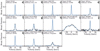 |
Fig. C.1 Broadening functions for the single-lined systems. The black curves show the broadening function from the highest S/N HPF spectrum. The blue curve shows a rotationally broadened line profile accounting for the resolution of HPF of 55,000, using the best-fit v sin i⋆ listed in Table 1. |
Appendix D ZTF light curves
Figure D.1, in the left-hand panels, shows the ZTF zg-band light-curves of several targets with unknown Prot values. The righthand panels show the corresponding Lomb-Scargle periodograms, which reveal the Prot for targets 2MASS J09481615+5114518, LSPM J1024+3902E, and GJ 3861. The data for 2MASS 10534129+5253040 was not precise enough to constrain its rotation period. Figure D.2 shows the same ZTF zg-band data for 2MASS J09481615+5114518, LSPM J1024+3902E, and GJ 3861, but phase-folded according to the period peak found in the Lomb–Scargle analysis.
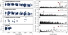 |
Fig. D.1 ZTF zg-band photometry of a) 2MASS J09481615+5114518, b) LSPM J1024+3902E, c) 2MASS J10534129+5253040, and d) GJ 3861. Panels e), f), g) and h) show the corresponding Lomb–Scargle periodograms. The gray vertical dashed lines show the 0.1% false alarm probability, and the red dots highlight the highest peaks with false alarms lower than 0.1% probability. |
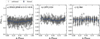 |
Fig. D.2 The phase-folded ZTF zg-band photometry of a) 2MASS J09481615+5114518, b) LSPM J1024+3902E, and c) GJ 3861, where we use the periodicities found through the Lomb–Scargle periodograms shown in Fig D.1. |
All Tables
The median S/N (in the 5th order index), median radial velocity error () of the HPF observations, as well as measurements of various activity and multiplicity indicators.
GJ 3861 RVs. v1 and σ1 lists the RVs and corresponding uncertainties of the primary star, and v2 and σ2 list the rvs RVs and uncertainties of the secondary star.
All Figures
|
Fig. 1 Broadening functions of the targets that showed significant evidence being spectroscopic multiples, i.e., showed evidence of two lines (GJ 3861 and GJ 9552), or three lines (GJ 3729). We additionally show GJ 3789, and G 240-45 which do not show a double line profile in the HPF broadening functions, but are known binary systems with close (<1.7″) companions (Beuzit et al. 2004; El-Badry et al. 2021). Finally, we also show the broadening function of 2MASS J10534129+5253040, which has a high Gaia DR3 RUWE value of 2.4, which we thus assume to be a close visual binary. The blue curves show a best-fit Gaussian to the primary (i.e. brightest) peak, the red curve shows the secondary peak (if any), and the yellow peak highlights a fit to a tertiary peak (if any). The GJ 3789 broadening function is multiplied by a factor of 10 in the y-axis for enhanced readability. |
| In the text | |
|
Fig. 2 19 radio M dwarfs studied in this work, along with the designations adopted from this work (Table 2). Targets are designated according to activity and multiplicity, and overplotted on a) a color–magnitude diagram, where we use the Gaia Catalogue of Nearby Stars (Gaia Collaboration 2021) to indicate the main sequence in gray, and b) the empirical Güdel–Benz relation (as described in Williams et al. 2014) with the 1σ spread indicated in the surrounding gray shaded region. The target G 240-45 is hereby not shown on the color–magnitude diagram, as its color is not listed in Gaia. The names of the suggested best MSPI candidates are all listed, and the systems GJ 625 and GJ 3861 – which are further discussed in Sections 4 and 5 – are highlighted in bold. |
| In the text | |
|
Fig. 3 ΔBIC periodograms of GJ 625, for the 1-planet vs. 0-planet model. The orange horizontal line shows our adopted False Alarm Probability (FAP) detection threshold of 0.1%, showing that the 14.6 d signal is significantly detected at ΔBIC ~ 55. The stellar rotation period (Prot = 80 ± 8 d) is indicated in yellow. |
| In the text | |
|
Fig. 4 RV observations of GJ 625. (A) RV time series of all available data of GJ 625, color-coded by spectrograph. (B) Phase folded RV data of GJ 625 phase-folded on the best-fit period of our model of 14.6288 days. The color coding is the same as in the plot on the left. Binned RV points are overplotted in red. The best-fit Keplerian model is shown in black. |
| In the text | |
|
Fig. 5 a) Wilson plot of GJ 3861’s RVs, showing the primary RV (RV1) as a function of the secondary RV (RV2). The best-fit line (red line) suggests a mass ratio of q = 0.767 ± 0.002, and a velocity offset of γ = −15.092 ± 0.029 km/s. b) Perpendicular distance residuals to the best-fit line shown in a). |
| In the text | |
|
Fig. 6 a) Periodogram of the primary star RVs of GJ 3861. The highest peak corresponding to a period of 14.855 days is highlighted with the red dot. The 1-day aliases of the best-fit period are highlighted with the red dashed lines. b) HPF RVs of the GJ 3861 binary system. Red and blue points show the RVs of the primary and secondary, respectively. The best-fit model is shown with the red and blue curves for the primary and secondary, respectively. c) Residuals from the best-fit. RV error bars are shown with the best-fit jitter values applied in quadrature. |
| In the text | |
|
Fig. 7 Stellar inclinations (cos i⋆) of the subsample where we have v sin i⋆, R⋆, and Prot measurements. Left shows the cos i⋆ over the stellar effective temperature. Right shows a histogram of the cos i⋆ values. The distribution of stellar inclinations is indistinguishable from an isotropic distribution. |
| In the text | |
|
Fig. 8 Upper limit for the Alfvénic Mach number of the stellar wind at the orbit of GJ 625 b as a function of the average large-scale surface magnetic field strength of the host star. The gray shaded regions show where the field strength is outside the likely estimate of the magnetic field of the star from 17 to 189 G, estimated from empirical relationships. For average field strengths ≳20 G, we estimate that the planet must orbit inside the Alfvén surface, corresponding to a Mach number <1 (indicated by the dashed horizontal line). In this region (highlighted in blue), magnetic star-planet interactions can occur. However, 3D MHD simulations are needed to assess these prospects further. |
| In the text | |
|
Fig. 9 Deviation of targets from the Güdel–Benz relation (Williams et al. 2014). The targets originally used to define this relation are shown in red, gray and blue. Coherently emitting, active targets detected with LOFAR – shown as black triangles and primarily consisting of RS CVn systems – scatter around the Güdel–Benz relation with a comparable spread (Vedantham et al. 2022). Our system, GJ 3861, is also indicated. |
| In the text | |
|
Fig. B.1 HPF observations of the Ca II IRT line at 8664 Å for all non-SB2 targets in the M dwarf radio sample (blue curves), compared to a single high S/N as-observed HPF spectrum of slowly rotating quiescent reference stars (black). The reference spectrum is rotationally broadened to match the observed broadening of the lines, by using the estimates of the v sin i obtained by HPF-SpecMatch. The red shaded region marks the line center, which is the emission window used to compute the Equivalent Width. The lower panels show the normalized ratio residuals (target/reference), highlighting any excess emission as a peak in the residuals. A continuum region (8670.300–8673.190 Å, gray shaded) is used to normalize the residuals to unity. The lower panels also denote our overall Ca II IRT emission designation, as either ‘Low’ |
| In the text | |
|
Fig. C.1 Broadening functions for the single-lined systems. The black curves show the broadening function from the highest S/N HPF spectrum. The blue curve shows a rotationally broadened line profile accounting for the resolution of HPF of 55,000, using the best-fit v sin i⋆ listed in Table 1. |
| In the text | |
|
Fig. D.1 ZTF zg-band photometry of a) 2MASS J09481615+5114518, b) LSPM J1024+3902E, c) 2MASS J10534129+5253040, and d) GJ 3861. Panels e), f), g) and h) show the corresponding Lomb–Scargle periodograms. The gray vertical dashed lines show the 0.1% false alarm probability, and the red dots highlight the highest peaks with false alarms lower than 0.1% probability. |
| In the text | |
|
Fig. D.2 The phase-folded ZTF zg-band photometry of a) 2MASS J09481615+5114518, b) LSPM J1024+3902E, and c) GJ 3861, where we use the periodicities found through the Lomb–Scargle periodograms shown in Fig D.1. |
| In the text | |
Current usage metrics show cumulative count of Article Views (full-text article views including HTML views, PDF and ePub downloads, according to the available data) and Abstracts Views on Vision4Press platform.
Data correspond to usage on the plateform after 2015. The current usage metrics is available 48-96 hours after online publication and is updated daily on week days.
Initial download of the metrics may take a while.