| Issue |
A&A
Volume 706, February 2026
|
|
|---|---|---|
| Article Number | A256 | |
| Number of page(s) | 16 | |
| Section | Interstellar and circumstellar matter | |
| DOI | https://doi.org/10.1051/0004-6361/202556981 | |
| Published online | 17 February 2026 | |
Characterizing the physical and chemical properties of the Class I protostellar system Oph-IRS 44
Binarity, infalling streamers, and accretion shocks
1
European Southern Observatory,
Alonso de Córdova 3107, Casilla 19, Vitacura,
Santiago,
Chile
2
Instituto de Astrofísica, Pontificia Universidad Católica de Chile,
Av. Vicuña Mackenna 4860,
7820436
Macul, Santiago,
Chile
3
Millennium Nucleus on Young Exoplanets and their Moons (YEMS),
Chile
4
Leiden Observatory, Leiden University,
PO Box 9513,
2300RA
Leiden,
The Netherlands
5
Department of Astronomy, University of Michigan,
1085 S. University Ave.,
Ann Arbor,
MI
48109,
USA
6
Institute of Astronomy, Department of Physics, National Tsing Hua University,
Hsinchu,
Taiwan
7
RIKEN Cluster for Pioneering Research,
2-1, Hirosawa, Wako-shi,
Saitama
351-0198,
Japan
8
Niels Bohr Institute, University of Copenhagen,
Øster Voldgade 5–7,
1350
Copenhagen,
Denmark
★ Corresponding author: This email address is being protected from spambots. You need JavaScript enabled to view it.
Received:
25
August
2025
Accepted:
16
December
2025
Abstract
Context. In the low-mass star formation process, theoretical models predict that material from the infalling envelope could be shocked as it encounters the outer regions of the disk. This is followed by an increase in the dust temperature and sublimation, into the gas phase, of molecular species that will otherwise remain locked on dust grains. Although accretion shocks are predicted by theoretical models, only a few protostars show evidence of these shocks at the disk-envelope interface, and the main formation path of shocked-related species is still unclear. They can be formed entirely on dust surfaces and then sublimated, or through reactions in the gas phase, or a combination of both.
Aims. The goal of this work is to assess the chemistry associated with accretion shocks and the formation path of molecules that are usually associated with these dense and warm regions.
Methods. We present new observations of IRS 44, a Class I source with a resolved disk that has previously been associated with accretion shocks, taken at high angular resolution (0⋅′′1, corresponding to 14 au) with the Atacama Large Millimeter/submillimeter Array (ALMA). We observe three different spectral settings in bands 6 and 7, targeting multiple molecular transitions of CO, H2CO, and simple sulfur-bearing species (such as CS, SO, SO2, H2S, OCS, and H2CS).
Results. In continuum emission, the binary nature of IRS 44 is observed for the first time at sub-millimeter wavelengths and the emission agrees with the optical and infrared counterparts. Infalling signatures are seen for the CO 2–1 line and the emission peaks at the edges of the continuum emission around IRS 44 B, the same region where bright SO and SO2 emission is seen. Weak CS and H2CO emission is observed, while OCS, H2S, and H2CS transitions are not detected.
Conclusions. IRS 44 B seems to be more embedded than IRS 44 A, indicating a non-coeval formation scenario or the rejuvenation of source B due to late infall. CO 2–1 emission is tracing the outflow component at large scales, infalling envelope material at intermediate scales, and two infalling streamer candidates are identified at disk scales. Infalling streamers might produce accretion shocks when they encounter the outer regions of the infalling-rotating envelope. These shocks heat the dust and efficiently release S-bearing species (such as H2S, SO, and SO2), as well as promoting a lukewarm chemistry (~200 K) in the gas phase. With the majority of carbon locked in CO, there is little free C available to form CS and H2CS in the gas, leaving an oxygen-rich environment. The high column densities of SO and SO2 might therefore be a consequence of two processes: direct thermal desorption from dust grains and gas-phase formation due to the availability of O and S. IRS 44 is an ideal candidate with which to study the chemical consequences of accretion shocks and the dynamical connections between the envelope and the disk, through infalling streamers.
Key words: astrochemistry / protoplanetary disks / stars: formation / ISM: molecules / ISM: individual objects: Oph-IRS 44
© The Authors 2026
 Open Access article, published by EDP Sciences, under the terms of the Creative Commons Attribution License (https://creativecommons.org/licenses/by/4.0), which permits unrestricted use, distribution, and reproduction in any medium, provided the original work is properly cited.
This article is published in open access under the Subscribe to Open model. This email address is being protected from spambots. You need JavaScript enabled to view it. to support open access publication.
1 Introduction
The formation and evolution of low-mass protostars and their disks are fundamental to understanding the formation of our own Solar System. A typical low-mass star forms when a molecular cloud with angular momentum collapses, the central protostar accretes mass, material from the envelope infalls into the central regions, and a circumstellar disk forms in the equatorial plane (Cassen & Moosman 1981; Terebey et al. 1984; Shu et al. 1993; Hartmann 1998). Eventually, planets will form within the disk, and their final composition is strongly dependent on the physical and chemical processes within the circumstellar disk (e.g., Herbst & van Dishoeck 2009; Drozdovskaya et al. 2018; Jørgensen et al. 2020; Öberg et al. 2023; van ’t Hoff & Bergner 2024). In recent years, it has been found that infalling and accretion processes are not isotropic. How protostars accrete material from the surrounding envelope is still an open question (e.g., Pineda et al. 2023; Kuffmeier et al. 2023, 2020).
Theoretical models predict that streamer-like infall supply material from the envelope (or molecular cloud scales) onto the disk, and accretion shocks are created at the envelope-disk interface (Ulrich 1976; Mendoza et al. 2009; Kuffmeier et al. 2019). These shocks induce an increase in the temperature and species that formed in grain mantles are subsequently released into the gas phase, affecting the chemical evolution of the early disk and the material available for planet formation (van Dishoeck & Bergin 2021; van Gelder et al. 2021). The chemical content of the early disk could therefore be partially reset after the passage of the shock, whereas the absence of shocks suggests a chemical inheritance between the envelope and the disk. Despite being a natural consequence in theoretical models, only a few low-mass protostars show observational evidence of streamers and accretion shocks (e.g., Sakai et al. 2014; Yen et al. 2019; Pineda et al. 2020; Artur de la Villarmois et al. 2022; Garufi et al. 2022; Valdivia-Mena et al. 2022; Hsieh et al. 2023; Gupta et al. 2024; Liu et al. 2025). Furthermore, it is still not well understood if the observed shock-related species are being formed entirely on the dust surfaces and then sublimated, or if there is an important contribution to the formation of the molecule in the gas phase (van Gelder et al. 2021).
IRS 44, also known as YLW 16 (Young et al. 1986), is a Class I source located in the Ophiuchus molecular cloud, at a distance of 139 pc (average value for the L1688 cloud; Cánovas et al. 2019). It has been proposed that IRS 44 is a protobinary system with a separation of ![Mathematical equation: $\[0^{\prime\prime}_\cdot3\]$](/articles/aa/full_html/2026/02/aa56981-25/aa56981-25-eq2.png) , based on optical and infrared observations (Allen et al. 2002; Duchêne et al. 2007; Herczeg et al. 2011). Nevertheless, Sadavoy et al. (2019), Artur de la Villarmois et al. (2019), and Artur de la Villarmois et al. (2022) did not find any evidence of binarity in ALMA data at an angular resolution of
, based on optical and infrared observations (Allen et al. 2002; Duchêne et al. 2007; Herczeg et al. 2011). Nevertheless, Sadavoy et al. (2019), Artur de la Villarmois et al. (2019), and Artur de la Villarmois et al. (2022) did not find any evidence of binarity in ALMA data at an angular resolution of ![Mathematical equation: $\[0^{\prime\prime}_\cdot25\]$](/articles/aa/full_html/2026/02/aa56981-25/aa56981-25-eq3.png) (35 au) in band 6,
(35 au) in band 6, ![Mathematical equation: $\[0^{\prime\prime}_\cdot4\]$](/articles/aa/full_html/2026/02/aa56981-25/aa56981-25-eq4.png) (56 au) in band 7, and
(56 au) in band 7, and ![Mathematical equation: $\[0^{\prime\prime}_\cdot1\]$](/articles/aa/full_html/2026/02/aa56981-25/aa56981-25-eq5.png) (14 au) in band 7, respectively. Strong and compact SO2 emission was first detected toward IRS 44 by Artur de la Villarmois et al. (2019) and, later on, IRS 44 was associated with accretion shocks through the detection of multiple SO2 transitions (Artur de la Villarmois et al. 2022). The latter work provided the following physical properties for the inner regions of IRS 44 (≤50 au): H2 densities higher than 108 cm−3, SO2 rotational temperatures between 90 and 250 K, and high SO2 column densities of between 0.4 and 1.8 × 1017 cm−2. IRS 44 is therefore a suitable source in which to search for other sulfur-bearing species, assess the main formation path of SO2, and understand the chemistry related to accretion shocks and potential infalling streamers.
(14 au) in band 7, respectively. Strong and compact SO2 emission was first detected toward IRS 44 by Artur de la Villarmois et al. (2019) and, later on, IRS 44 was associated with accretion shocks through the detection of multiple SO2 transitions (Artur de la Villarmois et al. 2022). The latter work provided the following physical properties for the inner regions of IRS 44 (≤50 au): H2 densities higher than 108 cm−3, SO2 rotational temperatures between 90 and 250 K, and high SO2 column densities of between 0.4 and 1.8 × 1017 cm−2. IRS 44 is therefore a suitable source in which to search for other sulfur-bearing species, assess the main formation path of SO2, and understand the chemistry related to accretion shocks and potential infalling streamers.
In this paper we present high-angular-resolution ![Mathematical equation: $\[0^{\prime\prime}_\cdot1\]$](/articles/aa/full_html/2026/02/aa56981-25/aa56981-25-eq6.png) (14 au) ALMA observations of multiple molecular transitions toward IRS 44, most of them related with sulfur-bearing species. Section 2 describes the observational procedure, calibration, and CO 2–1 archival data. The observational results are presented in Sect. 3, together with the observed molecular transitions and the interpretation of a streamer candidate. Section 4 is dedicated to the analysis of the data, with the estimation of temperatures and column densities. We discuss the chemistry related to IRS 44 in Sect. 5, and end with a summary in Sect. 6.
(14 au) ALMA observations of multiple molecular transitions toward IRS 44, most of them related with sulfur-bearing species. Section 2 describes the observational procedure, calibration, and CO 2–1 archival data. The observational results are presented in Sect. 3, together with the observed molecular transitions and the interpretation of a streamer candidate. Section 4 is dedicated to the analysis of the data, with the estimation of temperatures and column densities. We discuss the chemistry related to IRS 44 in Sect. 5, and end with a summary in Sect. 6.
Parameters of the continuum observations after applying self-calibration.
2 Observations
IRS 44 was observed with ALMA during April, May, and June 2023 as part of the program 2022.1.00209.S (PI: Elizabeth Artur de la Villarmois). At the time of the observations, between 30 and 44 antennas were available in the array providing baselines between 15 and 3697 m. The observations targeted three different spectral settings – two of them in band 7 and one in band 6 – to observe multiple transitions of sulfur-bearing species, CO isotopologs, and H2CO. These lines are presented and discussed in Sect. 3.2.
The calibration and imaging were done in CASA1 pipeline version 6.4.1 (McMullin et al. 2007). Gain and bandpass calibrations were performed through the observation of the quasars J1554–2704, J1617–2537, and J1700–2610. Imaging was performed using the tclean task in CASA, where the Briggs weighting with a robust parameter of 0.5 was employed. The automasking option was chosen and the velocity resolution is 0.2 km s−1. Self-calibration was performed only for the continuum data, where the final solution intervals, central frequencies, beam size, and root mean square (rms) values are listed in Table 1 for the three spectral settings. The largest angular scale (LAS) of these observations is ~![Mathematical equation: $\[1^{\prime\prime}_\cdot2\]$](/articles/aa/full_html/2026/02/aa56981-25/aa56981-25-eq7.png) for both bands, band 6 and band 7, as band 6 was observed in configuration C43-7 and band 7 in C43-6.
for both bands, band 6 and band 7, as band 6 was observed in configuration C43-7 and band 7 in C43-6.
Archival ALMA data
Only one data cube was retrieved from the ALMA archive, which corresponds to the CO 2–1 transition that is part of project 2019.1.01792.S (PI: Diego Mardones). We took the product cube from the archive, without additional calibration or cleaning. The synthesized beam is ![Mathematical equation: $\[1^{\prime\prime}_\cdot2\]$](/articles/aa/full_html/2026/02/aa56981-25/aa56981-25-eq8.png) ×
× ![Mathematical equation: $\[0^{\prime\prime}_\cdot9\]$](/articles/aa/full_html/2026/02/aa56981-25/aa56981-25-eq9.png) , the LAS is
, the LAS is ![Mathematical equation: $\[5^{\prime\prime}_\cdot0\]$](/articles/aa/full_html/2026/02/aa56981-25/aa56981-25-eq10.png) , and the rms is 0.016 Jy beam−1. The main purpose of retrieving this cube was to assess the CO intermediate spatial scales (between
, and the rms is 0.016 Jy beam−1. The main purpose of retrieving this cube was to assess the CO intermediate spatial scales (between ![Mathematical equation: $\[1^{\prime\prime}_\cdot0\]$](/articles/aa/full_html/2026/02/aa56981-25/aa56981-25-eq11.png) and
and ![Mathematical equation: $\[5^{\prime\prime}_\cdot0\]$](/articles/aa/full_html/2026/02/aa56981-25/aa56981-25-eq12.png) ) that are filtered out in our data (LAS =
) that are filtered out in our data (LAS = ![Mathematical equation: $\[1^{\prime\prime}_\cdot0\]$](/articles/aa/full_html/2026/02/aa56981-25/aa56981-25-eq13.png) ), but this dataset was not used in the analysis. The red- and blueshifted contours for the archival data are presented in Appendix B.
), but this dataset was not used in the analysis. The red- and blueshifted contours for the archival data are presented in Appendix B.
3 Results
3.1 Continuum emission
IRS 44: A proto-binary
The continuum emission is shown in Fig. 1, for three different frequencies (233.0, 303.0, and 328.2 GHz). Source A is clearly detected in ALMA band 6, with a signal-to-noise ratio (S/N) of around 60, while the S/N decreases for shorter wavelengths (S/N = 14 and 6 for 303.0 and 328.2 GHz, respectively). Although the peak intensity increases for band 7 observations, the rms does as well, decreasing the S/N (see Table 2). The integrated and peak flux were calculated using two-dimensional (2D) Gaussian fits in the image plane. Furthermore, the protostellar disk mass, Mdisk, was calculated for both sources, using the following equation:
![Mathematical equation: $\[M_{\mathrm{disk}}=\frac{S_\nu d^2}{\kappa_\nu B_\nu(T)},\]$](/articles/aa/full_html/2026/02/aa56981-25/aa56981-25-eq14.png) (1)
(1)
where Sν represents the surface brightness, d the distance to the source, κν the dust opacity, and Bν(T) the Planck function for a single temperature. The adopted dust temperature (Tdust) is 15 K (see Dunham et al. 2014), and the derived masses (gas + dust, assuming a gas-to-dust ratio of 100) are listed in Table 3. We find that the disk around source B is 10 times more massive than that of source A. Additionally, there is a difference between the disk mass around source B for different wavelengths, where the highest value corresponds to the longer wavelength. This discrepancy hints at optically thick emission, mainly at 303.0 and 328.2 GHz, but the continuum emission at 233.0 GHz might also suffer from optical depth effects (to a lesser degree). Therefore, Mdisk should be taken as a lower limit.
Figure 2 shows the spectral energy distribution (SED) of IRS 44 as a system. Source A is brighter in the infrared regime (Terebey et al. 2001; Dunham et al. 2015), while the opposite situation is seen at sub-millimeter wavelengths where both components are resolved: source B is much brighter than source A. This suggests that (i) both sources are in different evolutionary stages, (ii) they have different orientations, or (iii) source B appears younger due to late infall (e.g., Kuffmeier et al. 2023). Murillo et al. (2016) found that 33% of multiple protostellar systems are non-coeval, mainly due to its formation history and different dynamical evolution. Given that a dark lane is observed along source B in optical images (see Fig. 2 in Terebey et al. 2001) and the fact that molecular transitions, such as CO, are not detected toward source A (e.g., Herczeg et al. 2011), a non-coeval scenario or a rejuvenation of source B due to late infall are the more plausible scenarios for the IRS 44 system. The binarity of IRS 44 is better seen in band 6 observations, which have been targeted before by Sadavoy et al. (2019) but with a poorer angular resolution (![Mathematical equation: $\[0^{\prime\prime}_\cdot25\]$](/articles/aa/full_html/2026/02/aa56981-25/aa56981-25-eq15.png) ) that is not enough to resolve both sources. On the other hand, Artur de la Villarmois et al. (2022) observed IRS 44 in band 7 (330 GHz) with the same angular resolution of
) that is not enough to resolve both sources. On the other hand, Artur de la Villarmois et al. (2022) observed IRS 44 in band 7 (330 GHz) with the same angular resolution of ![Mathematical equation: $\[0^{\prime\prime}_\cdot1\]$](/articles/aa/full_html/2026/02/aa56981-25/aa56981-25-eq16.png) ; however, the detection of source A was not clear, similar to in the right panel of Fig. 1.
; however, the detection of source A was not clear, similar to in the right panel of Fig. 1.
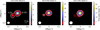 |
Fig. 1 Continuum emission of IRS 44 above 3σ at different frequencies. The white contour represents a flux value of 10σ. The synthesized beam is represented by a filled white ellipse in the lower left corner of each panel. IRS 44 A and B can also be found as IRS 44 E and W in the literature, respectively (e.g., Herczeg et al. 2011). |
Integrated and peak continuum fluxes for both sources.
Calculated disk masses for both sources, A and B, from the continuum fluxes.
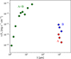 |
Fig. 2 Spectral energy distribution (SED) of IRS 44. In the infrared regime (green dots), the flux corresponds to both sources, source A being the brightest one (Terebey et al. 2001; Dunham et al. 2015). In ALMA bands, the binary system is resolved and source B (blue dots) is ~10 times brighter than source A (red dots). |
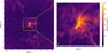 |
Fig. 3 CO 2–1 emission (moment 8) at large (left) and intermediate scales (right). The white stars represent the position of the A and B components (see Fig. 1). The synthesized beam is represented by a filled white ellipse in the lower left corner of each panel. |
3.2 Molecular transitions
The ALMA observations consist of three spectral settings targeting several molecular transitions, which are listed in Table A.1. CO isotopologs, SO, 34SO, and SO2, are among the detected species, together with CS and only one clear detection of H2CO. On the other hand, transitions from 34SO2, OCS, H2S, and H2CS are not detected at a 3σ level.
Figure 3 shows the moment 8 map (maximum value of the spectrum) of the CO 2–1 transition at large and intermediate scales. The same map is superimposed with the CO 2–1 velocity contours from the archival data (see Figure B.1 in the appendix), which has a larger beam size (![Mathematical equation: $\[1^{\prime\prime}_\cdot2\]$](/articles/aa/full_html/2026/02/aa56981-25/aa56981-25-eq17.png) ×
× ![Mathematical equation: $\[0^{\prime\prime}_\cdot9\]$](/articles/aa/full_html/2026/02/aa56981-25/aa56981-25-eq18.png) ) and a LAS of
) and a LAS of ![Mathematical equation: $\[5^{\prime\prime}_\cdot0\]$](/articles/aa/full_html/2026/02/aa56981-25/aa56981-25-eq19.png) . The CO emission seems to trace arc-like structures at small scales, closer to the binary system, an elongated envelope structure encompassing the arcs, and an extended component in the northeast-southwest direction. The latter component is consistent with the outflow direction (PA = 20°) observed by van der Marel et al. (2013) using single-dish observations of CO 3–2. Given that the LAS of our observations related to the moment 8 map is
. The CO emission seems to trace arc-like structures at small scales, closer to the binary system, an elongated envelope structure encompassing the arcs, and an extended component in the northeast-southwest direction. The latter component is consistent with the outflow direction (PA = 20°) observed by van der Marel et al. (2013) using single-dish observations of CO 3–2. Given that the LAS of our observations related to the moment 8 map is ![Mathematical equation: $\[1^{\prime\prime}_\cdot0\]$](/articles/aa/full_html/2026/02/aa56981-25/aa56981-25-eq20.png) , emission more extended than that value will be filtered out by the interferometer; therefore, only the densest regions are seen.
, emission more extended than that value will be filtered out by the interferometer; therefore, only the densest regions are seen.
3.2.1 Streamer candidates
The arc-like structures could potentially be associated with infalling streamers but, given that significant emission is filtered out, a kinematic analysis is needed. Figure 4 shows moment 8,0 and 1 maps for the CO 2–1 transition in a zoomed-in-on area. The moment 8 presents three main arc-like structures in the northwest, while only one prominent component is seen toward the southeast. The moment 0 map shows more compact emission, covering an area of ![Mathematical equation: $\[0^{\prime\prime}_\cdot6\]$](/articles/aa/full_html/2026/02/aa56981-25/aa56981-25-eq21.png) , and a weaker tail is observed toward the southeast. On the other hand, the moment 1 map exhibits a clear velocity gradient toward source B, with two main components. The redshifted one coincides with the prominent component seen toward the southeast in the moment 8 map, which we call the SE streamer candidate. The blueshifted emission correlates with only one of the two arc-like structures seen in the northern regions of source B (see moment 8 map), which is the proposed NW streamer candidate. This velocity gradient is likely due to infalling gas, as higher velocities are seen closer to the protostar; this is discussed in more detail in the next few paragraphs. The black-dashed curve in Fig. 4 represents the directions of the streamer candidates from this work, which are remarkably symmetric around the continuum peak of source B. A more detailed theoretical and kinematic analysis of the streamer candidates will be presented in a future work. The spectra and moment 0 maps of the CO isotopologs are shown in Fig. C.1 in the appendix.
, and a weaker tail is observed toward the southeast. On the other hand, the moment 1 map exhibits a clear velocity gradient toward source B, with two main components. The redshifted one coincides with the prominent component seen toward the southeast in the moment 8 map, which we call the SE streamer candidate. The blueshifted emission correlates with only one of the two arc-like structures seen in the northern regions of source B (see moment 8 map), which is the proposed NW streamer candidate. This velocity gradient is likely due to infalling gas, as higher velocities are seen closer to the protostar; this is discussed in more detail in the next few paragraphs. The black-dashed curve in Fig. 4 represents the directions of the streamer candidates from this work, which are remarkably symmetric around the continuum peak of source B. A more detailed theoretical and kinematic analysis of the streamer candidates will be presented in a future work. The spectra and moment 0 maps of the CO isotopologs are shown in Fig. C.1 in the appendix.
Figure 5 shows channel maps for the CO 2–1 emission, for ranges of 2 km s−1. Maps with mean velocities between −7 and −11 km s−1 show that the blueshifted emission extends to ~![Mathematical equation: $\[1^{\prime\prime}_\cdot0\]$](/articles/aa/full_html/2026/02/aa56981-25/aa56981-25-eq22.png) and approaches source B as the velocity increases, in agreement with infalling signatures. Additionally, more compact emission is seen for higher velocities, between −13 and −19 km s−1. Redshifted emission shows a similar behavior to that of negative velocities, but the emission is more confined toward the southeast.
and approaches source B as the velocity increases, in agreement with infalling signatures. Additionally, more compact emission is seen for higher velocities, between −13 and −19 km s−1. Redshifted emission shows a similar behavior to that of negative velocities, but the emission is more confined toward the southeast.
Position-velocity (PV) diagrams of CO 2–1 are shown in Fig. 6, for different position angles (PAs). Infalling signatures are seen in the blueshifted emission for all the PAs, and the weakest components are observed for PA = 60° and 80°, with negative offsets (i.e., to the east of the system). The redshifted emission is less clear than the blueshifted one, but shows an infalling profile for PA = 160° and the weakest emission for 60° ≤ PA ≤ 100°. The weak emission seen in PA = 40° located at ![Mathematical equation: $\[2^{\prime\prime}_\cdot0\]$](/articles/aa/full_html/2026/02/aa56981-25/aa56981-25-eq23.png) seems to trace a denser region of the outflow cavity wall. Note that the LAS of these observations is
seems to trace a denser region of the outflow cavity wall. Note that the LAS of these observations is ![Mathematical equation: $\[1^{\prime\prime}_\cdot0\]$](/articles/aa/full_html/2026/02/aa56981-25/aa56981-25-eq24.png) ; therefore, any extended structure beyond
; therefore, any extended structure beyond ![Mathematical equation: $\[1^{\prime\prime}_\cdot0\]$](/articles/aa/full_html/2026/02/aa56981-25/aa56981-25-eq25.png) is filtered out by the interferometer.
is filtered out by the interferometer.
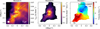 |
Fig. 4 CO 2–1 emission at small scales. Left: maximum value map (moment 8) above a 3σ level. Center: integrated map (moment 0) above a 15σ level (1σ = 10 mJy beam−1 km s−1). Right: velocity map (moment 1) above a 15σ level. The white contour represents the continuum emission at 233 GHz at a 10σ value and the dashed black curves indicate the direction of the proposed streamers. The synthesized beam is represented by a filled white ellipse in the left panel. |
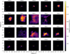 |
Fig. 5 Velocity channel maps for CO 2–1 above 1σ. The systemic velocity (3.7 km s−1) is shifted to zero and each map has a velocity width of 2 km s−1. The yellow stars show the position of IRS44 A and IRS44 B, while the synthesized beam is represented by a filled white ellipse in the upper left panel. |
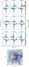 |
Fig. 6 Position–velocity (PV) diagrams for CO 2–1 (upper panels) above 3σ. The horizontal dashed red line represents the systemic velocity of 3.7 km s−1, while the vertical dashed blue line corresponds to the central position of source B. The different PAs (lower panel) are indicated by yellow lines over the CO 2–1 moment 8 map. |
3.2.2 SO and SO2 as tracers of accretion shocks
Figure 7 shows moment 0 and 1 maps for the brightest SO transition, 78–67 (Eu = 81.2 K), and SO2 222,20–221,21 (Eu = 248.0 K). The elongated structure seen toward the southeast in SO is consistent with the shocked region proposed by Artur de la Villarmois et al. (2022). Additionally, it matches the direction of the SE streamer candidate, seen in CO in Fig. 4. Unlike SO, the SO2 transition shows the peak of emission toward the south, within the continuum, but the velocity gradient also follows the direction of the SE streamer candidate.
Artur de la Villarmois et al. (2022) proposed that the SO2 emission toward IRS 44 is tracing accretion shocks, given the high temperatures (above 90 K) and high densities (≥108 cm−3) that were estimated by analyzing six SO2 and three 34SO2 transitions at an angular resolution of ![Mathematical equation: $\[0^{\prime\prime}_\cdot1\]$](/articles/aa/full_html/2026/02/aa56981-25/aa56981-25-eq26.png) . They proposed that the radius of the centrifugal barrier (rCB) is
. They proposed that the radius of the centrifugal barrier (rCB) is ![Mathematical equation: $\[0^{\prime\prime}_\cdot08\]$](/articles/aa/full_html/2026/02/aa56981-25/aa56981-25-eq27.png) , inside which the gas motion is expected to be Keplerian (e.g., Sakai et al. 2014; Oya et al. 2018). The rCB is half of the centrifugal radius (rCR), and infalling-rotation motions are present between both radii. Beyond rCR the gas is pure infall. The extents of the proposed rCB and rCR are shown in Fig. 8, where SO and SO2 emission is superimposed with the CO emission. The peak of the SO and SO2 emission is seen toward the edges of the rCB, and most of the emission arises from the region where rotating-infalling motions were proposed.
, inside which the gas motion is expected to be Keplerian (e.g., Sakai et al. 2014; Oya et al. 2018). The rCB is half of the centrifugal radius (rCR), and infalling-rotation motions are present between both radii. Beyond rCR the gas is pure infall. The extents of the proposed rCB and rCR are shown in Fig. 8, where SO and SO2 emission is superimposed with the CO emission. The peak of the SO and SO2 emission is seen toward the edges of the rCB, and most of the emission arises from the region where rotating-infalling motions were proposed.
Artur de la Villarmois et al. (2022) only targeted one SO transition; therefore, the physical properties of the SO emitting gas was estimated from the SO2 results. Here we targeted five SO transitions, plus two 34SO lines (see Table A.1). The SO line with the lowest Eu (15.8 K; 10–01) is the weakest one, showing some hint of emission in its spectrum (see Fig. C.2 in Appendix C.2), but its moment 0 map is very noisy. On the other hand, the brightest SO line toward IRS 44 is the one with the highest Eu value (81.2 K) and quantum numbers, 78–67. Note that the SO transition most commonly observed with ALMA in band 6 (65–54 and Eu = 35.0 K; within the CO spectral setting) is clearly detected, but not the brightest one toward IRS 44. Spectra and moment 0 maps for S-bearing species are presented in Appendix C.2, in Fig. C.2.
4 Analysis
Excitation temperatures and molecular column densities
Apart from CO isotopologs, where the emission appears to be optically thick, SO is the only species with multiple transitions clearly detected. Thus, the SO physical parameters were estimated by comparing a grid of models with observed line ratios. For CO, CS, H2CO, OCS, H2S, and H2CS, column densities were calculated assuming a range of temperatures, and values for SO2 and CH3OH were taken from the literature (Artur de la Villarmois et al. 2022, 2019).
4.1 SO
To estimate the excitation temperature (Tex) and molecular column densities of SO (NSO), we employed the non-local thermodynamic equilibrium (LTE) radiative transfer code RADEX and compared the models with the observed intensity ratios between the four SO transitions clearly detected (see Table A.1 and Fig. C.2). Energy levels, transitions frequencies, and Einstein A coefficients were taken from the Cologne Database for Molecular Spectroscopy (CDMS), while collisional rates were taken from Lique et al. (2006). The details of the RADEX models are presented in Appendix D. The observed intensity ratios (see Fig. D.1) allow us to discard nH = 106 cm−3, given that there is no range of temperatures and densities that contains the observed line ratios (see Fig. D.2). For nH = 107 cm−3 and nH = 108 cm−3, kinetic temperatures (Tkin) of between 50 and 220 K are possible, while NSO ranges between 0.06 and 7.0 × 1017 cm−2 (see Fig. D.2). We note that temperatures above 220 K are not shown in Fig. D.2, but this upper limit was chosen given that gas-phase SO2 formation is more efficient at temperatures below 200 K (see Sect. 5.1). At Tkin = 300 K, nH increases slightly, up to 8.0 × 1017 cm−2. Table 4 shows a wide range for Tkin and NSO, but these limits could be reduced with future observations of SO transitions with higher Eu values.
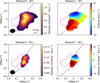 |
Fig. 7 SO and SO2 emission. Upper panels: moment 0 and 1 maps for SO 78–67 above 5σ. Lower panels: moment 0 and 1 maps for SO2 222,20–221,21 above 5σ. The magenta contour represents the continuum emission at 233 GHz at a 10σ value and the dashed black curves indicate the direction of the proposed streamers. The synthesized beam is represented by a filled black ellipse in the left panels. |
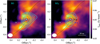 |
Fig. 8 CO (moment 8) emission in colorscale superimposed with SO (left) and SO2 (right) contours from moment 0 maps (in steps of 5σ). The dashed black curves indicate the direction of the proposed streamers. The dashed black and blue circles represent the extent of the centrifugal barrier and centrifugal radius, respectively, from Artur de la Villarmois et al. (2022). The synthesized beam is represented by a filled white ellipse. |
4.2 CO, CS, and H2CO
CO isotopologs are usually optically thick and absorption features are seen in their spectra (see Fig. C.1 in the appendix); thus, NCO was estimated from 13CO 3–2 and assuming a range of excitation temperatures (50–200 K). Assuming LTE conditions, the following equation was employed:
![Mathematical equation: $\[N=\frac{N_{\mathrm{u}}}{g_{\mathrm{u}}} Q\left(T_{\mathrm{ex}}\right) \exp \left(\frac{E_{\mathrm{u}}}{T_{\mathrm{ex}}}\right),\]$](/articles/aa/full_html/2026/02/aa56981-25/aa56981-25-eq28.png) (2)
(2)
where Nu is the column density of the upper level, gu the level degeneracy, Eu the energy of the upper level in kelvin, N the total column density of the molecule, and Q(Tex) the partition function that depends on the excitation temperature.
Nu was obtained from
![Mathematical equation: $\[N_{\mathrm{u}}=\frac{4 \pi S_\nu \Delta v}{A_{i j} \Omega h c},\]$](/articles/aa/full_html/2026/02/aa56981-25/aa56981-25-eq29.png) (3)
(3)
where Sν.Δv is the integrated flux density, Aij the Einstein A coefficient, Ω the solid angle covered by the integrated area, h the Planck constant, and c the speed of light. Equation (3) can be rewritten as
![Mathematical equation: $\[N_{\mathrm{u}}=2375 \times 10^6\left(\frac{S_\nu \Delta v}{1 ~\mathrm{Jy} \mathrm{~km} \mathrm{~s}^{-1}}\right)\left(\frac{1 \mathrm{~s}^{-1}}{A_{i j}}\right)\left(\frac{\operatorname{arcsec}^2}{\Theta_{\text {area }}}\right),\]$](/articles/aa/full_html/2026/02/aa56981-25/aa56981-25-eq30.png) (4)
(4)
where Θarea is the area of integration and Nu was obtained in particles per square centimeter. Equations (2) and (4) were used to estimate the total column density for CO, CS, and H2CO, over a circular region with r = ![Mathematical equation: $\[0^{\prime\prime}_\cdot5\]$](/articles/aa/full_html/2026/02/aa56981-25/aa56981-25-eq31.png) , and assuming a range of Tex between 50 and 200 K. The calculated values are listed in Table 4.
, and assuming a range of Tex between 50 and 200 K. The calculated values are listed in Table 4.
Excitation temperature and molecular column densities.
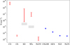 |
Fig. 9 Molecular column densities. Values are taken from Table 4, where red bars represent the estimated ranges and blue triangles indicate upper limits. Horizontal gray bars represent average values (±1σ) from Class I sources in the Perseus star-forming region (Artur de la Villarmois et al. 2023). |
4.3 OCS, H2S, and H2CS
For non-detections, an integrated flux equivalent to 3σ was employed in Equation (4), and calculated column densities should be interpreted as upper limits. In cases in which more than one transition was targeted (such as OCS and H2S), the line with the highest Aij was selected to estimate the total molecular column density. Temperatures and molecular column densities are presented in Table 4 and Fig. 9.
5 Discussion
In this section, we interpret the presence of bright lines from species, such as SO and SO2, and the absence (or weak emission) of other targeted transitions.
5.1 Bright SO and SO2
Artur de la Villarmois et al. (2023) analyzed the SO and SO2 emission of a sample of 14 Class I sources in the Perseus star-forming region, and estimated the SO and SO2 column densities of eight and five sources, respectively. They found average values of 2.5 × 1015 cm−2 for SO (from SO 66–55 and 34SO 56–45 multiplied by 22) and 9.9 × 1014 cm−2 for SO2 140,14–131,13. The only Class I hot-corino source, Per-emb 44, was not included in this calculation, as it shows optically thick SO and SO2 emission. Figure 9 shows that the SO and SO2 column densities toward IRS 44 are higher than the average values from the Perseus sources (represented by the horizontal gray bars). The lower limit estimated for NSO toward IRS 44 is slightly higher than that from the Perseus sources; however, for NSO2 the values toward IRS 44 are considerable higher (about two orders of magnitude) than the mean value toward the Perseus sources. These high values might be a consequence of gas-phase reactions, direct desorption from dust grains, or a combination of both processes. The main reactions for SO and SO2 formation in the gas phase are
![Mathematical equation: $\[\begin{aligned}& \mathrm{S}+\mathrm{OH} \rightarrow \mathrm{SO}+\mathrm{H}, \\& \mathrm{~S}+\mathrm{O}_2 \rightarrow \mathrm{SO}+\mathrm{O},\end{aligned}\]$](/articles/aa/full_html/2026/02/aa56981-25/aa56981-25-eq36.png) (5)
(5)
and
![Mathematical equation: $\[\mathrm{SO}+\mathrm{OH} \rightarrow \mathrm{SO}_2+\mathrm{H}.\]$](/articles/aa/full_html/2026/02/aa56981-25/aa56981-25-eq37.png) (6)
(6)
Reaction (6) is more efficient at temperatures below 200 K (Charnley 1997), where the presence of OH in the gas phase is required. Karska et al. (2018) did not detect OH toward IRS 44 from Herschel/PACS observations, but infrared observations are more sensitive to optically thin and extended warm gas. Additionally, if the OH emitting region is comparable to the SO one (≤![Mathematical equation: $\[0^{\prime\prime}_\cdot5\]$](/articles/aa/full_html/2026/02/aa56981-25/aa56981-25-eq38.png) ), the emission will be diluted within the Herschel beam area, and therefore not detectable. Thus the presence of OH cannot be ruled out.
), the emission will be diluted within the Herschel beam area, and therefore not detectable. Thus the presence of OH cannot be ruled out.
Another possibility for the high column densities of SO and SO2 is the direct desorption from dust grains. When the infalling material encounters the outer regions of the disk, it generates accretion shocks, increasing the dust temperature and releasing molecules to the gas phase. The broad spectra seen for SO and SO2 (from −15 to 15 km s−1) with multiple peaks at different velocities (see Fig. C.2) suggest that the SO and SO2 emission is tracing shocked regions. van Gelder et al. (2021) estimated that, for a density of 108 cm−3, the sublimation temperatures of SO2 and SO are 62 K and 37 K, respectively. Additionally, they modeled accretion shocks at the disk envelope interface and concluded that desorption of SO2 ice is efficient in high-density environments (≥108 cm−3) and shock velocities of ≥10 km s−1. These values are consistent with the H2 number density found by Artur de la Villarmois et al. (2022), nH ≥ 108 cm−3, and with the velocity gradient seen in Figs 4 and 7. Therefore, some degree of direct SO2 desorption is expected toward IRS 44.
5.2 Shocks: Origins of S-bearing species and efficient production of H2O
Atomic sulfur is also required in the gas phase to form SO via Reaction (5). Anderson et al. (2013) studied the S I abundance in shocked gas with Spitzer observations and found that atomic sulfur is a major reservoir of sulfur in shocked gas. Sulfur would be present is some form that is released from grains as atoms, perhaps via sputtering, within the shock. Once in the gas phase, atomic sulfur can be converted into a molecular form, or ionized on rapid timescales of ~60/G0 yr (where G0 = 1 is the interstellar radiation field; Habing 1968). Recent works have proposed that sulfur is locked into dust grains in the form of organosulfur species (Laas & Caselli 2019), sulfide minerals such as FeS (Kama et al. 2019), sulfur chains such as S8 (Shingledecker et al. 2020; Cazaux et al. 2022), and adsorption of S+ followed by grain surface chemistry (Fuente et al. 2023).
Apart from direct SO and SO2 sublimation, van Gelder et al. (2021) propose that H2O is efficiently produced in shocks with velocities ≥4 km s−1 through the reaction of OH with H2. In addition, in dense environments (nH ≥ 107 cm−3), these shocks will thermally desorb H2S for Tdust = 47 K. Once in the gas phase, if the UV radiation intensity is large enough (G0) ≥ 10, H2O photodissociates into OH + H and photodissociation of H2S significantly increases the abundance of atomic S and SH. The latter is also involved in the formation of SO and S via
![Mathematical equation: $\[\begin{aligned}& \mathrm{SH}+\mathrm{O} \rightarrow \mathrm{SO}+\mathrm{H}, \\& \mathrm{SH}+\mathrm{H} \rightarrow \mathrm{~S}+\mathrm{H}_2.\end{aligned}\]$](/articles/aa/full_html/2026/02/aa56981-25/aa56981-25-eq39.png) (7)
(7)
Photodissociation of H2S and H2O will therefore increase the OH, S, and SH abundances, promoting SO and SO2 formation in the gas phase (Reactions (5), (6), and (7)).
The L1688 cloud in the Ophiuchus star-forming region harbors a rich cluster of young stellar objects (YSOs) at various evolutionary stages and two OB stars (HD 147889 and ρ Oph A; Wilking & Lada 1983). The UV intensity, G0, ranges between 100 and 1000 in the L1688 cloud, reaching its maximum value around the OB stars (Rawlings et al. 2013; Xia et al. 2022). These values are in agreement with the condition needed to photodissociate H2O and H2S (i.e., G0 ≥ 10).
5.3 Weak CS and H2CO
The main destruction path of SO is the reaction with atomic carbon (Bergin et al. 1997):
![Mathematical equation: $\[\mathrm{SO}+\mathrm{C} \rightarrow \mathrm{CS}+\mathrm{O},\]$](/articles/aa/full_html/2026/02/aa56981-25/aa56981-25-eq40.png) (8)
(8)
where an increase in the CS abundance is expected. However, CS is very weak around the inner regions (≤50 au) of IRS 44, its emission peak is slightly offset (~![Mathematical equation: $\[0^{\prime\prime}_\cdot15\]$](/articles/aa/full_html/2026/02/aa56981-25/aa56981-25-eq41.png) or 20 au) from the redshifted emission of SO and SO2 (see Fig. C.2), and its spectrum shows a narrow peak. This suggests that CS is not tracing the same material as SO and SO2, but it might be present in the more quiescent and extended envelope associated with IRS 44, which is probably also filtered out by the interferometer. The weak CS in the shocked gas might imply that most of the atomic carbon is locked into CO and Reaction (8) is inefficient.
or 20 au) from the redshifted emission of SO and SO2 (see Fig. C.2), and its spectrum shows a narrow peak. This suggests that CS is not tracing the same material as SO and SO2, but it might be present in the more quiescent and extended envelope associated with IRS 44, which is probably also filtered out by the interferometer. The weak CS in the shocked gas might imply that most of the atomic carbon is locked into CO and Reaction (8) is inefficient.
The low column density found for H2CO reflects its weak emission, where only one transition (out of nine; see Fig. C.3) is clearly detected. The Eu values of the targeted H2CO transitions range from 21 to 174 K, and the detected line corresponds to Eu = 47.9 K. This suggests that H2CO may be present in the cold envelope at large scales, and not in the shocked regions closer to the protostar. H2CO can directly sublimate from dust grains for Tdust ≥ 65 K (van Gelder et al. 2021) but it is also formed in the gas phase for temperatures below 100 K (Loomis et al. 2015; van’t Hoff et al. 2020; Guzmán et al. 2021) via
![Mathematical equation: $\[\mathrm{CH}_{3}+\mathrm{O} \rightarrow \mathrm{H}_{2} \mathrm{CO}+\mathrm{H}.\]$](/articles/aa/full_html/2026/02/aa56981-25/aa56981-25-eq42.png) (9)
(9)
Independently of the formation route, the weak H2CO emission suggests that this molecule is being destroyed around the inner regions (≤50 au) of IRS 44. van Gelder et al. (2021) proposed that H2CO is destroyed by S+ in shocked gas, forming CO + H2S+ or SH + HCO+. The less abundant isotopolog, H13CO+, was detected in the inner regions of IRS 44 (≤150 au; Artur de la Villarmois et al. 2019), indicating that H2CO destruction by S+ might be efficient. In this scenario, the SH abundance would also increase, and Reaction (7) will once more become efficient and promote the formation of S and SO.
5.4 Absence of OCS and CH3OH
Boogert et al. (2022) and Santos et al. (2024) found a good correlation between the ice abundances of OCS and CH3OH in massive young stellar objects (MYSOs). If this correlation is also valid for low-mass YSOs, the OCS non-detection in the gas phase toward IRS 44 agrees with the absence of CH3OH emission (Artur de la Villarmois et al. 2019). If OCS and CH3OH are abundant in the ices toward IRS 44, their non-detections in the gas phase would suggest that (i) the physical conditions related to accretion shocks are not sufficient to release them to the gas phase, or (ii) they desorb from dust grains but get destroyed after sublimation. Suutarinen et al. (2014) proposed that CH3OH is destroyed by shocks with moderate velocities (≥10 km s−1), where the main products are H + CH2OH. In the absence of C species (other than CO), the main destruction path for OCS in the gas phase is by HCO+ (OCS + HCO+ → HOCS+ + CO) or by ![Mathematical equation: $\[\mathrm{H}_{3}^{+}\]$](/articles/aa/full_html/2026/02/aa56981-25/aa56981-25-eq43.png) (OCS +
(OCS + ![Mathematical equation: $\[\mathrm{H}_{3}^{+}\]$](/articles/aa/full_html/2026/02/aa56981-25/aa56981-25-eq44.png) → HOCS+ + H2), as has been pointed out by el Akel et al. (2022). Additional observations are needed to explain the OCS and CH3OH non-detections.
→ HOCS+ + H2), as has been pointed out by el Akel et al. (2022). Additional observations are needed to explain the OCS and CH3OH non-detections.
5.5 Very low CS/SO
The CS/SO column density ratio has been shown to be sensitive to the overall C/O ratio in the gas in Class II disks (i.e., Semenov et al. 2018; Le Gal et al. 2021). In IRS 44, the low CS/SO ratio (≤0.008) is a consequence of the weak CS emission. As is shown in Fig. C.2 in the appendix, the CS emission peaks toward the south of IRS 44 B, slightly offset (~![Mathematical equation: $\[0^{\prime\prime}_\cdot15\]$](/articles/aa/full_html/2026/02/aa56981-25/aa56981-25-eq45.png) or 20 au) from the redshifted peak of SO and SO2, and 13CS and C34S are not detected, ruling out the possibility that the CS 7–6 transition is optically thick. The low CS/SO ratio is consistent with the values toward IRS 48 (CS/SO < 0.01; Booth et al. 2024), but in high contrast with C/O ratios estimated for Class II disks (≥2.0; Bosman et al. 2021; Le Gal et al. 2021). CS/SO ratios toward younger and more embedded Class I disks are unknown in general, given the challenge of distinguishing between the different components of the system. For example, CS is commonly tracing the disk and also more extended emission from the outflow and envelope components (Artur de la Villarmois et al. 2023). Thus, high-angular-resolution observations and multiple transitions are essential for an accurate CS/SO estimation toward embedded sources.
or 20 au) from the redshifted peak of SO and SO2, and 13CS and C34S are not detected, ruling out the possibility that the CS 7–6 transition is optically thick. The low CS/SO ratio is consistent with the values toward IRS 48 (CS/SO < 0.01; Booth et al. 2024), but in high contrast with C/O ratios estimated for Class II disks (≥2.0; Bosman et al. 2021; Le Gal et al. 2021). CS/SO ratios toward younger and more embedded Class I disks are unknown in general, given the challenge of distinguishing between the different components of the system. For example, CS is commonly tracing the disk and also more extended emission from the outflow and envelope components (Artur de la Villarmois et al. 2023). Thus, high-angular-resolution observations and multiple transitions are essential for an accurate CS/SO estimation toward embedded sources.
Another Class I source with bright SO and SO2 emission, but no detection of CS, is Per-emb 50 (Artur de la Villarmois et al. 2023). This is the only source within a sample of 50 Class 0/I YSOs that shows this behavior and it has been associated with accretion shocks (Zhang et al. 2023) and an infalling streamer (Valdivia-Mena et al. 2022). This may suggest that the CS intensity anticorrelates with the presence of accretion shocks.
The fact that CS and sometimes H2CS are the main sulfur-bearing molecules detected in Class II disks (Le Gal et al. 2019; Law et al. 2025) may suggest that H2CS in Class II disks is likely forming in the gas phase at low temperatures (<100 K; Booth et al. 2024), while SO and SO2 are detected in those sources where infalling material is still significant (e.g., Garufi et al. 2022) or the UV radiation can heat the dust to temperatures where SO and SO2 can thermally desorb (Booth et al. 2021). From the discussion above, the physical conditions that seem to prevail toward the inner regions (≤![Mathematical equation: $\[0^{\prime\prime}_\cdot3\]$](/articles/aa/full_html/2026/02/aa56981-25/aa56981-25-eq46.png) or 40 au) of IRS 44 are the following: Tgas between 100 and 300 K, nH ≥ 107 cm−3, a shock velocity of ≥4 km s−1, and G0 ≥ 10.
or 40 au) of IRS 44 are the following: Tgas between 100 and 300 K, nH ≥ 107 cm−3, a shock velocity of ≥4 km s−1, and G0 ≥ 10.
Figure 10 shows a schematic representation of the inner regions of IRS 44 and our interpretation of the data. Infalling streamers are producing accretion shocks when they encounter the outer regions of the infalling-rotating envelope. These shocks heat the dust and efficiently release S-bearing species (such as S, H2S, SO, and SO2), as well as promoting a lukewarm chemistry (~200 K) in the gas phase. Most of the atomic carbon might be locked into CO, so there is no available C to form CS and H2CS, which leaves an oxygen-rich environment. The high column densities of SO and SO2 might therefore be a consequence of both processes: direct thermal desorption from dust grains and gas-phase formation due to the availability of O- and S-bearing species. Finally, a Keplerian disk is expected in the innermost regions associated with IRS 44 B (≤![Mathematical equation: $\[0^{\prime\prime}_\cdot08\]$](/articles/aa/full_html/2026/02/aa56981-25/aa56981-25-eq47.png) or 11 au).
or 11 au).
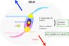 |
Fig. 10 Schematic representation of the IRS 44 system. Infalling streamers produce accretion shocks in the outer regions of the rotating-infalling envelope and a Keplerian disk is expected in the innermost regions of IRS 44 B. Most of the C is locked into CO; thus, CS and H2CS formation is not efficient. Accretion shocks sublimate S-bearing species and enhance their gas abundances, promoting a lukewarm chemistry (~200 K) in the gas phase, mainly involving O- and S-bearing species. |
6 Summary
This work presents new ALMA data toward the Class I source IRS 44, where multiple molecular transitions are targeted, sulfur-bearing species being the most relevant ones. The main results are summarized below:
The continuum emission shows a binary component, which is brighter in ALMA band 6 (233.0 GHz). The binarity of IRS 44 was proposed before from infrared observations; nevertheless, this is the first time that the binary components have been resolved in the sub-millimeter regime. The average total disk masses (dust + gas) calculated for source B and source A are 5.1 × 10⁻³ and 0.53 × 10⁻³ M⊙, respectively, with one order of magnitude difference between them;
Among the CO-bearing species, 12CO, 13CO, and C18O transitions are detected; however, only one H2CO line is clearly detected at small scales. Colder H2CO might be more abundant at larger and more extended scales;
For S-bearing species, six SO transitions are clearly detected (including two 34SO), while only the most abundant isotopologs of CS and SO2 are detected. The targeted OCS, H2S, and H2CS transitions are not detected in this dataset;
The envelope around IRS 44 shows infalling signatures (mainly seen in CO emission) and, as the gas approaches the disk, an S shape stands out in the velocity profile of CO. This S shape, or arc-like structures, represent our streamer candidates and the direction of the southeast one agrees with the slightly extended redshifted emission seen in SO. The infalling streamers would generate accretion shocks when the material encounters the outer regions of the rotating-infalling envelope;
We propose that the high SO and SO2 column densities are driven by two main physical mechanisms: direct thermal desorption from dust grains due to the accretion shocks and gas-phase formation within the O-rich gaseous environment present in the inner regions of IRS 44 B;
Accretion shocks seem to be essential to increase the gas abundance of S, H2S, SO, and SO2, as well as forming H2O in the gas phase. Later on, atomic sulfur can be ionized, while H2S, and H2O could be photodissociated, increasing the abundance of S+, S, SH, O, and OH; the main reactants of SO and SO2;
The weak CS emission will be explained by the lack of atomic C available in the gas, where CO formation depletes the available carbon and an oxygen-rich chemistry is promoted. H2CO might be destroyed in the shocked gas by S+, which explains its weak emission. Nevertheless, both CS and H2CO are expected to be abundant in the colder and more extended envelope around the IRS 44 system;
The absence of OCS is in agreement with the non-detection of CH3OH, as both species seem to share a common origin in ice mantles. If OCS and CH3OH are abundant in the ices toward IRS 44, those species remain locked and the physical conditions related to accretion shocks are not sufficient to release them to the gas phase, or they are both thermally desorbed and later on destroyed in the gas phase;
Weak CS emission, absence of COMs, and bright SO and SO2 emission seem to be a good recipe for accretion shocks with moderate velocities (~10 km s−1) toward embedded sources;
We propose that the physical conditions toward the inner regions (≤
![Mathematical equation: $\[0^{\prime\prime}_\cdot3\]$](/articles/aa/full_html/2026/02/aa56981-25/aa56981-25-eq48.png) or 40 au) of IRS 44 are the following: Tgas between 100 and 300 K, nH ≥ 107 cm−3, a shock velocity of ≥4 km s−1, and G0 ≥ 10.
or 40 au) of IRS 44 are the following: Tgas between 100 and 300 K, nH ≥ 107 cm−3, a shock velocity of ≥4 km s−1, and G0 ≥ 10.
IRS 44 is an ideal candidate with which to study the chemical consequences of accretion shocks and the complex dynamics of young and embedded proto-binary systems. Future observations of H218O, HDO, and OH would allow us to test our proposed scenario, while continuum ALMA observations of the dust with a higher angular resolution (≤![Mathematical equation: $\[0^{\prime\prime}_\cdot1\]$](/articles/aa/full_html/2026/02/aa56981-25/aa56981-25-eq49.png) ) and in multiple bands would allow us to better constrain the disk’s physical properties and the dust temperature, which is expected to increase in shocked regions. There are other S-bearing species that are not targeted in these observations, such as CCS, NS, NS+, and salts such as NH4SH (e.g., Slavicinska et al. 2025). Given the weak CS emission and non-detection of H2CS, CCS is not expected to be abundant, however, N-bearing species containing sulfur and salts could constitute an important sulfur sink. Future estimations of the CS/SO ratio toward a larger sample of more embedded disks would provide valuable information on the material transport and the chemical evolution from younger to more evolved disks.
) and in multiple bands would allow us to better constrain the disk’s physical properties and the dust temperature, which is expected to increase in shocked regions. There are other S-bearing species that are not targeted in these observations, such as CCS, NS, NS+, and salts such as NH4SH (e.g., Slavicinska et al. 2025). Given the weak CS emission and non-detection of H2CS, CCS is not expected to be abundant, however, N-bearing species containing sulfur and salts could constitute an important sulfur sink. Future estimations of the CS/SO ratio toward a larger sample of more embedded disks would provide valuable information on the material transport and the chemical evolution from younger to more evolved disks.
Acknowledgements
We thank the anonymous referee for a number of good suggestions that helped us to improve this work. This paper makes use of the following ALMA data: ADS/JAO.ALMA#2022.0.00209.S and ADS/JAO.ALMA#2019.1.01792.S. ALMA is a partnership of ESO (representing its member states), NSF (USA) and NINS (Japan), together with NRC (Canada), MOST and ASIAA (Taiwan), and KASI (Republic of Korea), in cooperation with the Republic of Chile. The Joint ALMA Observatory is operated by ESO, AUI/NRAO and NAOJ. The National Radio Astronomy Observatory is a facility of the National Science Foundation operated under cooperative agreement by Associated Universities, Inc. V.V.G. acknowledge support from the ANID – Millennium Science Initiative Program – Center Code NCN2024_001, from FONDECYT Regular 1221352, and ANID CATA-BASAL project FB210003. D.H. is supported by the Ministry of Education of Taiwan (Center for Informatics and Computation in Astronomy grant and grant number 110J0353I9) and the National Science and Technology Council, Taiwan (Grant NSTC111-2112-M-007-014-MY3, NSTC113-2639-M-A49-002-ASP, and NSTC113-2112-M-007-027).
References
- Allen, L. E., Myers, P. C., Di Francesco, J., et al. 2002, ApJ, 566, 993 [NASA ADS] [CrossRef] [Google Scholar]
- Anderson, D. E., Bergin, E. A., Maret, S., & Wakelam, V. 2013, ApJ, 779, 141 [Google Scholar]
- Artur de la Villarmois, E., Jørgensen, J. K., Kristensen, L. E., et al. 2019, A&A, 626, A71 [NASA ADS] [CrossRef] [EDP Sciences] [Google Scholar]
- Artur de la Villarmois, E., Guzmán, V. V., Jørgensen, J. K., et al. 2022, A&A, 667, A20 [NASA ADS] [CrossRef] [EDP Sciences] [Google Scholar]
- Artur de la Villarmois, E., Guzmán, V. V., Yang, Y. L., Zhang, Y., & Sakai, N. 2023, A&A, 678, A124 [NASA ADS] [CrossRef] [EDP Sciences] [Google Scholar]
- Bergin, E. A., Goldsmith, P. F., Snell, R. L., & Langer, W. D. 1997, ApJ, 482, 285 [NASA ADS] [CrossRef] [Google Scholar]
- Boogert, A. C. A., Brewer, K., Brittain, A., & Emerson, K. S. 2022, ApJ, 941, 32 [NASA ADS] [CrossRef] [Google Scholar]
- Booth, A. S., van der Marel, N., Leemker, M., van Dishoeck, E. F., & Ohashi, S. 2021, A&A, 651, L6 [NASA ADS] [CrossRef] [EDP Sciences] [Google Scholar]
- Booth, A. S., Temmink, M., van Dishoeck, E. F., et al. 2024, AJ, 167, 165 [NASA ADS] [CrossRef] [Google Scholar]
- Bosman, A. D., Alarcón, F., Bergin, E. A., et al. 2021, ApJS, 257, 7 [NASA ADS] [CrossRef] [Google Scholar]
- Cánovas, H., Cantero, C., Cieza, L., et al. 2019, A&A, 626, A80 [NASA ADS] [CrossRef] [EDP Sciences] [Google Scholar]
- Cassen, P., & Moosman, A. 1981, Icarus, 48, 353 [CrossRef] [Google Scholar]
- Cazaux, S., Carrascosa, H., Muñoz Caro, G. M., et al. 2022, A&A, 657, A100 [NASA ADS] [CrossRef] [EDP Sciences] [Google Scholar]
- Charnley, S. B. 1997, ApJ, 481, 396 [NASA ADS] [CrossRef] [Google Scholar]
- Drozdovskaya, M. N., van Dishoeck, E. F., Jørgensen, J. K., et al. 2018, MNRAS, 476, 4949 [Google Scholar]
- Duchêne, G., Bontemps, S., Bouvier, J., et al. 2007, A&A, 476, 229 [Google Scholar]
- Dunham, M. M., Vorobyov, E. I., & Arce, H. G. 2014, MNRAS, 444, 887 [NASA ADS] [CrossRef] [Google Scholar]
- Dunham, M. M., Allen, L. E., Evans, II, N. J., et al. 2015, ApJS, 220, 11 [NASA ADS] [CrossRef] [Google Scholar]
- el Akel, M., Kristensen, L. E., Le Gal, R., et al. 2022, A&A, 659, A100 [CrossRef] [EDP Sciences] [Google Scholar]
- Fuente, A., Rivière-Marichalar, P., Beitia-Antero, L., et al. 2023, A&A, 670, A114 [NASA ADS] [CrossRef] [EDP Sciences] [Google Scholar]
- Garufi, A., Podio, L., Codella, C., et al. 2022, A&A, 658, A104 [CrossRef] [EDP Sciences] [Google Scholar]
- Gupta, A., Miotello, A., Williams, J. P., et al. 2024, A&A, 683, A133 [NASA ADS] [CrossRef] [EDP Sciences] [Google Scholar]
- Guzmán, V. V., Bergner, J. B., Law, C. J., et al. 2021, ApJS, 257, 6 [CrossRef] [Google Scholar]
- Habing, H. J. 1968, Bull. Astron. Inst. Netherlands, 19, 421 [Google Scholar]
- Hartmann, L. 1998, Cambr. Astrophys. Ser., 32 [Google Scholar]
- Herbst, E., & van Dishoeck, E. F. 2009, ARA&A, 47, 427 [Google Scholar]
- Herczeg, G. J., Brown, J. M., van Dishoeck, E. F., & Pontoppidan, K. M. 2011, A&A, 533, A112 [NASA ADS] [CrossRef] [EDP Sciences] [Google Scholar]
- Hsieh, T. H., Segura-Cox, D. M., Pineda, J. E., et al. 2023, A&A, 669, A137 [NASA ADS] [CrossRef] [EDP Sciences] [Google Scholar]
- Jørgensen, J. K., Belloche, A., & Garrod, R. T. 2020, ARA&A, 58, 727 [Google Scholar]
- Kama, M., Shorttle, O., Jermyn, A. S., et al. 2019, ApJ, 885, 114 [Google Scholar]
- Karska, A., Kaufman, M. J., Kristensen, L. E., et al. 2018, ApJS, 235, 30 [NASA ADS] [CrossRef] [Google Scholar]
- Kuffmeier, M., Calcutt, H., & Kristensen, L. E. 2019, A&A, 628, A112 [NASA ADS] [CrossRef] [EDP Sciences] [Google Scholar]
- Kuffmeier, M., Goicovic, F. G., & Dullemond, C. P. 2020, A&A, 633, A3 [NASA ADS] [CrossRef] [EDP Sciences] [Google Scholar]
- Kuffmeier, M., Jensen, S. S., & Haugbølle, T. 2023, Eur. Phys. J. Plus, 138, 272 [NASA ADS] [CrossRef] [Google Scholar]
- Laas, J. C., & Caselli, P. 2019, A&A, 624, A108 [NASA ADS] [CrossRef] [EDP Sciences] [Google Scholar]
- Law, C. J., Le Gal, R., Yamato, Y., et al. 2025, ApJ, 985, 84 [Google Scholar]
- Le Gal, R., Öberg, K. I., Loomis, R. A., Pegues, J., & Bergner, J. B. 2019, ApJ, 876, 72 [Google Scholar]
- Le Gal, R., Öberg, K. I., Teague, R., et al. 2021, ApJS, 257, 12 [NASA ADS] [CrossRef] [Google Scholar]
- Lique, F., Dubernet, M.-L., Spielfiedel, A., & Feautrier, N. 2006, A&A, 450, 399 [NASA ADS] [CrossRef] [EDP Sciences] [Google Scholar]
- Liu, X.-C., van Dishoeck, E. F., Hogerheijde, M. R., et al. 2025, A&A, 701, A141 [NASA ADS] [CrossRef] [EDP Sciences] [Google Scholar]
- Loomis, R. A., Cleeves, L. I., Öberg, K. I., Guzman, V. V., & Andrews, S. M. 2015, ApJ, 809, L25 [Google Scholar]
- McMullin, J. P., Waters, B., Schiebel, D., Young, W., & Golap, K. 2007, in Astronomical Society of the Pacific Conference Series, 376, Astronomical Data Analysis Software and Systems XVI, eds. R. A. Shaw, F. Hill, & D. J. Bell, 127 [Google Scholar]
- Mendoza, S., Tejeda, E., & Nagel, E. 2009, MNRAS, 393, 579 [NASA ADS] [CrossRef] [Google Scholar]
- Murillo, N. M., van Dishoeck, E. F., Tobin, J. J., & Fedele, D. 2016, A&A, 592, A56 [NASA ADS] [CrossRef] [EDP Sciences] [Google Scholar]
- Öberg, K. I., Facchini, S., & Anderson, D. E. 2023, ARA&A, 61, 287 [Google Scholar]
- Ossenkopf, V., & Henning, T. 1994, A&A, 291, 943 [NASA ADS] [Google Scholar]
- Oya, Y., Sakai, N., Watanabe, Y., et al. 2018, ApJ, 863, 72 [NASA ADS] [CrossRef] [Google Scholar]
- Pineda, J. E., Segura-Cox, D., Caselli, P., et al. 2020, Nat. Astron., 4, 1158 [NASA ADS] [CrossRef] [Google Scholar]
- Pineda, J. E., Arzoumanian, D., Andre, P., et al. 2023, in Astronomical Society of the Pacific Conference Series, 534, Protostars and Planets VII, eds. S. Inutsuka, Y. Aikawa, T. Muto, K. Tomida, & M. Tamura, 233 [Google Scholar]
- Rawlings, M. G., Juvela, M., Lehtinen, K., Mattila, K., & Lemke, D. 2013, MNRAS, 428, 2617 [Google Scholar]
- Sadavoy, S. I., Stephens, I. W., Myers, P. C., et al. 2019, ApJS, 245, 2 [Google Scholar]
- Sakai, N., Sakai, T., Hirota, T., et al. 2014, Nature, 507, 78 [Google Scholar]
- Santos, J. C., van Gelder, M. L., Nazari, P., Ahmadi, A., & van Dishoeck, E. F. 2024, A&A, 689, A248 [NASA ADS] [CrossRef] [EDP Sciences] [Google Scholar]
- Semenov, D., Favre, C., Fedele, D., et al. 2018, A&A, 617, A28 [NASA ADS] [CrossRef] [EDP Sciences] [Google Scholar]
- Shingledecker, C. N., Lamberts, T., Laas, J. C., et al. 2020, ApJ, 888, 52 [Google Scholar]
- Shu, F., Najita, J., Galli, D., Ostriker, E., & Lizano, S. 1993, in Protostars and Planets III, eds. E. H. Levy, & J. I. Lunine, 3 [Google Scholar]
- Slavicinska, K., Boogert, A. C. A., Tychoniec, Ł., et al. 2025, A&A, 693, A146 [NASA ADS] [CrossRef] [EDP Sciences] [Google Scholar]
- Suutarinen, A. N., Kristensen, L. E., Mottram, J. C., Fraser, H. J., & van Dishoeck, E. F. 2014, MNRAS, 440, 1844 [Google Scholar]
- Terebey, S., Shu, F. H., & Cassen, P. 1984, ApJ, 286, 529 [Google Scholar]
- Terebey, S., van Buren, D., Hancock, T., et al. 2001, in Astronomical Society of the Pacific Conference Series, 243, From Darkness to Light: Origin and Evolution of Young Stellar Clusters, eds. T. Montmerle, & P. André, 243 [Google Scholar]
- Ulrich, R. K. 1976, ApJ, 210, 377 [Google Scholar]
- Valdivia-Mena, M. T., Pineda, J. E., Segura-Cox, D. M., et al. 2022, A&A, 667, A12 [NASA ADS] [CrossRef] [EDP Sciences] [Google Scholar]
- van der Marel, N., Kristensen, L. E., Visser, R., et al. 2013, A&A, 556, A76 [NASA ADS] [CrossRef] [EDP Sciences] [Google Scholar]
- van Dishoeck, E. F., & Bergin, E. A. 2021, in ExoFrontiers; Big Questions in Exoplanetary Science, ed. N. Madhusudhan, 14 [Google Scholar]
- van Gelder, M. L., Tabone, B., van Dishoeck, E. F., & Godard, B. 2021, A&A, 653, A159 [CrossRef] [EDP Sciences] [Google Scholar]
- van ’t Hoff, M. L. R., & Bergner, J. B. 2024, arXiv e-prints [arXiv:2410.23235] [Google Scholar]
- van’t Hoff, M. L. R., Harsono, D., Tobin, J. J., et al. 2020, ApJ, 901, 166 [Google Scholar]
- Wilking, B. A., & Lada, C. J. 1983, ApJ, 274, 698 [NASA ADS] [CrossRef] [Google Scholar]
- Wilson, T. L. 1999, Rep. Progr. Phys., 62, 143 [CrossRef] [Google Scholar]
- Xia, J., Tang, N., Zhi, Q., et al. 2022, Res. Astron. Astrophys., 22, 085017 [CrossRef] [Google Scholar]
- Yen, H.-W., Gu, P.-G., Hirano, N., et al. 2019, ApJ, 880, 69 [NASA ADS] [CrossRef] [Google Scholar]
- Young, E. T., Lada, C. J., & Wilking, B. A. 1986, ApJ, 304, L45 [NASA ADS] [CrossRef] [Google Scholar]
- Zhang, Z. E., Yang, Y.-l., Zhang, Y., et al. 2023, ApJ, 946, 113 [NASA ADS] [CrossRef] [Google Scholar]
Appendix A Molecular transitions
The targeted molecular transitions within three different spectral setting are present in Table A.1, where the detected lines are listed at the beginning.
Appendix B CO 2–1 from archival data
Given that our observations filtered-out emission more extended than ![Mathematical equation: $\[1^{\prime\prime}_\cdot0\]$](/articles/aa/full_html/2026/02/aa56981-25/aa56981-25-eq50.png) , we use archival data (project 2019.1.01792.S) that targeted the same CO 2–1 transition, to trace intermediate scales: from
, we use archival data (project 2019.1.01792.S) that targeted the same CO 2–1 transition, to trace intermediate scales: from ![Mathematical equation: $\[1^{\prime\prime}_\cdot0\]$](/articles/aa/full_html/2026/02/aa56981-25/aa56981-25-eq51.png) to
to ![Mathematical equation: $\[5^{\prime\prime}_\cdot0\]$](/articles/aa/full_html/2026/02/aa56981-25/aa56981-25-eq52.png) . This CO emission is presented in Fig. B.1 as contour maps, showing that the infalling envelope covers an angular extent of ~
. This CO emission is presented in Fig. B.1 as contour maps, showing that the infalling envelope covers an angular extent of ~![Mathematical equation: $\[6^{\prime\prime}_\cdot0\]$](/articles/aa/full_html/2026/02/aa56981-25/aa56981-25-eq53.png) (~800 au), and the blueshifted emission is brighter and more extended than the redshifted one. Additionally, weaker outflow components are also seen, where blue- and redshifted emission overlap in the northeast and southwest directions, supporting the interpretation that the disk is roughly edge-on and the outflow axis lies close to the plane of the sky.
(~800 au), and the blueshifted emission is brighter and more extended than the redshifted one. Additionally, weaker outflow components are also seen, where blue- and redshifted emission overlap in the northeast and southwest directions, supporting the interpretation that the disk is roughly edge-on and the outflow axis lies close to the plane of the sky.
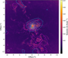 |
Fig. B.1 CO 2–1 emission at large scales. The colorscale represents the moment 8 map from this dataset, and the magenta and cyan contours show red- and blueshifted emission from archival data with poorer angular resolution and larger LAS. Magenta and cyan contours start at 60σ (1σ = 16 mJy beam−1 km s−1) and follow an increase of 125σ. The yellow stars represent the position of the A and B components (see Fig. 1) and the synthesized beams are represented by white ellipses in the lower-left corner of the map. |
Appendix C Spectra
Appendix C.1 CO isotopologs
All the targeted CO isotopolog transitions are detected, where the spectra and moment 0 maps are shown in Fig. C.1. For 13CO and C18O, two transitions are present in our spectral settings and, in both cases, the 3–2 transition is brighter than the 2–1 one. This suggests that the CO emitting region closer to the binary system is associated with more lukewarm temperatures (≥30 K). Furthermore, absorption features are seen toward the five spectra at the source velocity, indicating that extended emission is being filtered-out by the interferometer. Future observations of warmer CO transitions, such as 4–3 in band 8, would provide a better estimation of the gas temperature at disk scales.
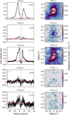 |
Fig. C.1 Emission of CO isotopologs. Left: Spectra taken from a region with a radius of |
![Mathematical equation: $\[0^{\prime\prime}_\cdot5\]$](/articles/aa/full_html/2026/02/aa56981-25/aa56981-25-eq54.png)
Appendix C.2 S-bearing species
Similarly to CO, spectra and moment 0 maps of SO, SO2 and CS isotopologs are shown in Fig. C.2. The brightest SO transition is the one with the highest Eu value (81.2 K), and all the spectra (with the exception of CS and 13CS) show similar profiles: a broad spectrum with brighter redshifted emission. The CS spectrum presents a bright and narrow redshifted peak. Although weak CS emission is seen at small scales, the integrated emission peaks toward the south of IRS 44 B, where SO and SO2 emission is significantly weak.
Spectral setup, parameters of the observed molecular transitions, and integrated line fluxes.
Appendix C.3 H2CO
Among the nine H2CO transitions, only one of them (41,3–31,2) is clearly detected, with an absorption and emission features at redshifted velocities. H2CO 30,3–20,2 and 40,4–30,3, the coldest transitions, present some hint of absorption, but this remains unclear.
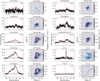 |
Fig. C.2 Same as Fig. C.1 for SO, SO2, and CS isotopologs. Weak lines, such as SO 12–01, SO 33–32, 34SO 67–56, 34SO 98–87, and SO2 222,20–221,21, have been multiplied by a factor of 2 or 3 for a better comparison. 13CS 5–4 is not detected in these data. |
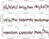 |
Fig. C.3 H2CO spectra taken from a region with a radius of |
![Mathematical equation: $\[0^{\prime\prime}_\cdot5\]$](/articles/aa/full_html/2026/02/aa56981-25/aa56981-25-eq58.png)
Appendix D Non-LTE radiative transfer models
The intensity ratios between the four brightest SO transitions are presented in Fig. D.1 and compared with RADEX models to estimate the kinetic temperature (Tkin) and SO column densities. The models are run for three different H2 number densities: 106, 107, and 108 cm−3. By comparing the observed intensity ratios with the RADEX models, the possible values are presented in Fig. D.2. The nH = 106 cm−3 scenario is discarded, given that there is no range of temperatures and densities that contain the three observed line ratios. For nH = 107 cm−3, and nH = 108 cm−3, kinetic temperatures (Tkin) between 50 and 220 K are possible, while NSO ranges between 0.06 and 7.0 × 1017 cm−2 (see Fig. D.2). We note that temperatures above 220 K are not shown in Fig. D.2, but this upper limit was chosen given that gas-phase SO2 formation is more efficient at temperatures below 200 K (see Sect. 5.1). At Tkin = 300 K, nH increases slightly, up to 8.0 × 1017 cm−2.
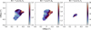 |
Fig. D.1 Observed intensity ratios between SO 78–67 and the other three bright SO transitions, above a 3σ level. |
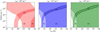 |
Fig. D.2 Range of possible values for the SO column density and the kinetic temperature (black contours) from the overlap of the observed intensity ratios in Fig. D.1, for three different values of the H2 number density. |
All Tables
Spectral setup, parameters of the observed molecular transitions, and integrated line fluxes.
All Figures
|
Fig. 1 Continuum emission of IRS 44 above 3σ at different frequencies. The white contour represents a flux value of 10σ. The synthesized beam is represented by a filled white ellipse in the lower left corner of each panel. IRS 44 A and B can also be found as IRS 44 E and W in the literature, respectively (e.g., Herczeg et al. 2011). |
| In the text | |
|
Fig. 2 Spectral energy distribution (SED) of IRS 44. In the infrared regime (green dots), the flux corresponds to both sources, source A being the brightest one (Terebey et al. 2001; Dunham et al. 2015). In ALMA bands, the binary system is resolved and source B (blue dots) is ~10 times brighter than source A (red dots). |
| In the text | |
|
Fig. 3 CO 2–1 emission (moment 8) at large (left) and intermediate scales (right). The white stars represent the position of the A and B components (see Fig. 1). The synthesized beam is represented by a filled white ellipse in the lower left corner of each panel. |
| In the text | |
|
Fig. 4 CO 2–1 emission at small scales. Left: maximum value map (moment 8) above a 3σ level. Center: integrated map (moment 0) above a 15σ level (1σ = 10 mJy beam−1 km s−1). Right: velocity map (moment 1) above a 15σ level. The white contour represents the continuum emission at 233 GHz at a 10σ value and the dashed black curves indicate the direction of the proposed streamers. The synthesized beam is represented by a filled white ellipse in the left panel. |
| In the text | |
|
Fig. 5 Velocity channel maps for CO 2–1 above 1σ. The systemic velocity (3.7 km s−1) is shifted to zero and each map has a velocity width of 2 km s−1. The yellow stars show the position of IRS44 A and IRS44 B, while the synthesized beam is represented by a filled white ellipse in the upper left panel. |
| In the text | |
|
Fig. 6 Position–velocity (PV) diagrams for CO 2–1 (upper panels) above 3σ. The horizontal dashed red line represents the systemic velocity of 3.7 km s−1, while the vertical dashed blue line corresponds to the central position of source B. The different PAs (lower panel) are indicated by yellow lines over the CO 2–1 moment 8 map. |
| In the text | |
|
Fig. 7 SO and SO2 emission. Upper panels: moment 0 and 1 maps for SO 78–67 above 5σ. Lower panels: moment 0 and 1 maps for SO2 222,20–221,21 above 5σ. The magenta contour represents the continuum emission at 233 GHz at a 10σ value and the dashed black curves indicate the direction of the proposed streamers. The synthesized beam is represented by a filled black ellipse in the left panels. |
| In the text | |
|
Fig. 8 CO (moment 8) emission in colorscale superimposed with SO (left) and SO2 (right) contours from moment 0 maps (in steps of 5σ). The dashed black curves indicate the direction of the proposed streamers. The dashed black and blue circles represent the extent of the centrifugal barrier and centrifugal radius, respectively, from Artur de la Villarmois et al. (2022). The synthesized beam is represented by a filled white ellipse. |
| In the text | |
|
Fig. 9 Molecular column densities. Values are taken from Table 4, where red bars represent the estimated ranges and blue triangles indicate upper limits. Horizontal gray bars represent average values (±1σ) from Class I sources in the Perseus star-forming region (Artur de la Villarmois et al. 2023). |
| In the text | |
|
Fig. 10 Schematic representation of the IRS 44 system. Infalling streamers produce accretion shocks in the outer regions of the rotating-infalling envelope and a Keplerian disk is expected in the innermost regions of IRS 44 B. Most of the C is locked into CO; thus, CS and H2CS formation is not efficient. Accretion shocks sublimate S-bearing species and enhance their gas abundances, promoting a lukewarm chemistry (~200 K) in the gas phase, mainly involving O- and S-bearing species. |
| In the text | |
|
Fig. B.1 CO 2–1 emission at large scales. The colorscale represents the moment 8 map from this dataset, and the magenta and cyan contours show red- and blueshifted emission from archival data with poorer angular resolution and larger LAS. Magenta and cyan contours start at 60σ (1σ = 16 mJy beam−1 km s−1) and follow an increase of 125σ. The yellow stars represent the position of the A and B components (see Fig. 1) and the synthesized beams are represented by white ellipses in the lower-left corner of the map. |
| In the text | |
|
Fig. C.1 Emission of CO isotopologs. Left: Spectra taken from a region with a radius of |
| In the text | |
|
Fig. C.2 Same as Fig. C.1 for SO, SO2, and CS isotopologs. Weak lines, such as SO 12–01, SO 33–32, 34SO 67–56, 34SO 98–87, and SO2 222,20–221,21, have been multiplied by a factor of 2 or 3 for a better comparison. 13CS 5–4 is not detected in these data. |
| In the text | |
|
Fig. C.3 H2CO spectra taken from a region with a radius of |
| In the text | |
|
Fig. D.1 Observed intensity ratios between SO 78–67 and the other three bright SO transitions, above a 3σ level. |
| In the text | |
|
Fig. D.2 Range of possible values for the SO column density and the kinetic temperature (black contours) from the overlap of the observed intensity ratios in Fig. D.1, for three different values of the H2 number density. |
| In the text | |
Current usage metrics show cumulative count of Article Views (full-text article views including HTML views, PDF and ePub downloads, according to the available data) and Abstracts Views on Vision4Press platform.
Data correspond to usage on the plateform after 2015. The current usage metrics is available 48-96 hours after online publication and is updated daily on week days.
Initial download of the metrics may take a while.