| Issue |
A&A
Volume 706, February 2026
|
|
|---|---|---|
| Article Number | A3 | |
| Number of page(s) | 15 | |
| Section | Cosmology (including clusters of galaxies) | |
| DOI | https://doi.org/10.1051/0004-6361/202557229 | |
| Published online | 27 January 2026 | |
Foreground removal in HI 21 cm intensity mapping under frequency-dependent beam distortions
1
Institutes of Computer Science and Astrophysics, Foundation for Research and Technology Hellas (FORTH), Greece
2
Université Paris-Saclay, Université Paris Cité, CEA, CNRS, AIM 91191 Gif-sur-Yvette, France
3
Observatoire de la Côte d’Azur, Laboratoire Lagrange, Bd de l’Observatoire, CS 34229 F-06304 Nice Cedex 4, France
4
Department of Physics and Astronomy, University of the Western Cape, Bellville Cape Town 7535, South Africa
5
Institute of Computer Science, Foundation for Research and Technology Hellas (FORTH), Greece
6
Department of Computer Science, University of Crete 71500 Heraklion, Greece
★ Corresponding author: This email address is being protected from spambots. You need JavaScript enabled to view it.
Received:
12
September
2025
Accepted:
15
November
2025
Abstract
Context. Neutral hydrogen (HI) intensity mapping with single-dish experiments is a powerful approach for probing cosmology in the post-reionization epoch. It is challenging to extract it, however, because of the bright foregrounds, which are stronger than the HI signal by more than four orders of magnitude. While all methods perform well when a Gaussian beam is assumed that is degraded to the lowest resolution, most methods degrade significantly in a more realistic beam model.
Aims. The complexity introduced by frequency-dependent beam effects means that we need methods that explicitly account for the instrument response. We investigate the performance of SDecGMCA. This method extends DecGMCA to spherical data by combining sparse component separation with beam deconvolution. Our goal is to evaluate this method in comparison with established foreground removal techniques by assessing its ability to recover the cosmological HI signal from single-dish intensity mapping observations under varying beam conditions.
Methods. We used simulated HI signals and foregrounds informed by existing observational and theoretical models that cover the frequency ranges relevant to MeerKAT and SKA-Mid. The foreground removal techniques we tested fall into two main categories: model-fitting methods (polynomial and parametric), and blind source separation methods (PCA, ICA, GMCA, and SDecGMCA). Their effectiveness was evaluated based on the recovery of the HI angular and frequency power spectra under progressively more realistic beam conditions.
Results. While all methods performed adequately under a uniform degraded beam, SDecGMCA remained robust when frequency-dependent beam distortions were introduced. For an oscillating beam, SDecGMCA suppressed the spurious spectral peak at kν ∼ 0.3 and achieved an accuracy of ≲5% at intermediate angular scales (10 < ℓ < 200); it outperformed other methods. Furthermore, the masking of bright Galactic regions significantly improved the recovery of the HI signal, in particular, for SDecGMCA, which benefited most when contaminated lines of sight were excluded. The beam inversion, however, remained intrinsically unstable beyond ℓ ∼ 200. This sets a practical limit on the method.
Conclusions. Our findings highlight the limitations of simple fitting and standard blind source separation methods for realistic beam effects, and they establish SDecGMCA as a particularly promising approach for future single-dish intensity mapping surveys. Its robustness for various beam models, combined with the improvements that can be achieved through masking strategies and forthcoming refinements to its thresholding scheme, suggest that SDecGMCA might provide reliable spherical harmonics reconstructions of the HI power spectrum in upcoming experiments.
Key words: methods: statistical / cosmology: observations / large-scale structure of Universe / radio lines: general
© The Authors 2026
 Open Access article, published by EDP Sciences, under the terms of the Creative Commons Attribution License (https://creativecommons.org/licenses/by/4.0), which permits unrestricted use, distribution, and reproduction in any medium, provided the original work is properly cited.
This article is published in open access under the Subscribe to Open model. This email address is being protected from spambots. You need JavaScript enabled to view it. to support open access publication.
1. Introduction
Observations over wider cosmic volumes are required to achieve a higher precision in probing the large-scale structure of the Universe. One of the most promising probes for this purpose is the 21 cm emission line of neutral hydrogen (HI), which traces the distribution of matter across cosmic time (Furlanetto et al. 2006; Pritchard & Loeb 2012). Unlike optical tracers, the 21 cm line is not obscured by dust and offers a tomographic view of the Universe because the observed frequency directly maps to redshift.
The faint HI signal means that detecting individual galaxies in 21 cm emission beyond the local Universe remains observationally expensive and requires prohibitively long integration times (e.g., Fernández et al. 2016; Gogate et al. 2020). HI intensity mapping (IM, Battye et al. 2004; Santos et al. 2005; Chang et al. 2008; Peterson et al. 2009; Kovetz et al. 2017) circumvents this challenge by measuring the collective 21 cm emission from unresolved sources over large sky areas and broad frequency ranges (Battye et al. 2013; Bull et al. 2015). Although this technique sacrifices angular resolution, it enables fast surveys of cosmological volumes with an excellent redshift precision.
Several experiments targeting the post-reionization epoch have made significant progress in detecting the HI signal through intensity mapping. The Green Bank Telescope (GBT) has produced cross-correlation measurements with galaxy surveys at low redshift (Masui et al. 2013; Switzer et al. 2013; Wolz et al. 2017, 2022), while the Parkes radio telescope has reported similar results using data from HI Parkes All Sky Survey (HIPASS) and other galaxy catalogs (Anderson et al. 2018; Tramonte & Ma 2020; Li et al. 2021). More recently, the MeerKAT radio telescope (Cunnington et al. 2023; Carucci et al. 2025; MeerKLASS Collaboration 2025; Chen et al. 2025) and the Canadian Hydrogen Intensity Mapping Experiment (CHIME; Amiri et al. 2023, 2024) have added to the growing list of detections by primarily relying on cross-correlation or stacking techniques. Autocorrelation measurements of the HI power spectrum have also emerged, notably at z ∼ 0.32 and z ∼ 0.44 (Paul et al. 2023). Complementary work has placed upper limits on the signal (e.g., Mazumder et al. 2025). It remains a key goal for the field to achieve high-precision autocorrelation measurements of the cosmological HI power spectrum with well-controlled systematics.
One of the main challenges in HI intensity mapping is contamination from astrophysical foregrounds. Synchrotron emission from the Milky Way, free–free radiation, and extragalactic point sources outshine the HI signal by up to five orders of magnitude even at high Galactic latitudes (Santos et al. 2005; Jelić et al. 2008). These contaminants have a complex spatial and spectral structure, which already complicates separation from the cosmological signal.
In addition, instrumental systematics, in particular, the frequency-dependent primary beam, further complicate the problem. The beam response couples to the foregrounds and introduces artificial spectral features that can mimic the 21 cm signal (Matshawule et al. 2021). The situation is made worse when the beam shows a nonsmooth (e.g., oscillatory) frequency dependence, as measured for MeerKAT (Asad et al. 2021). Other departures from the idealized chromatic response, such as those caused by instrumental optics or imperfect beam characterization, have also been shown to introduce systematic distortions in simulations and real data (Shaw et al. 2015; Chen et al. 2025).
A variety of methods have been developed to address this challenge. One of the most widely used are blind source separation (BSS) techniques, which aim to separate the HI signal from foreground contamination without relying heavily on prior models. Techniques such as a principal component analysis (PCA), an independent component analysis (ICA), FastICA, and a generalized morphological component analysis (GMCA) have shown promising results in theory- and simulation-based studies (Liu & Tegmark 2011; Ansari et al. 2012; Chapman et al. 2012; Masui et al. 2013; Switzer et al. 2013; Wolz et al. 2014; Bigot-Sazy et al. 2015; Alonso et al. 2015; Shaw et al. 2015; Olivari et al. 2016; Zhang et al. 2016; Wolz et al. 2017; Carucci et al. 2020; Soares et al. 2022).
These BSS techniques, along with several model-fitting approaches, were systematically compared by Spinelli et al. (2021), who evaluated their performance under various beam configurations. They found that no method performs optimally across all regimes. Each technique exhibited specific limitations, including systematic offsets and artifacts arising from beam effects, or intrinsic properties of the foreground and HI signals.
With the rise of machine learning, there has been increasing interest in applying deep-learning techniques to foreground removal and HI signal reconstruction (Makinen et al. 2021; Ni et al. 2022; Acharya et al. 2023; Shi et al. 2024; Ni et al. 2025; Chen et al. 2024). These approaches have demonstrated notable success in simulation-based studies, often leveraging large datasets such as the Cosmology and Astrophysics with MachinE Learning Simulations (CAMELS) (Villaescusa-Navarro et al. 2021). Their reliance on high-fidelity training simulations makes them sensitive to mismatches between training and real-world data, however. An incomplete knowledge of astrophysical foregrounds or instrumental systematics can bias these methods and might compromise their robustness. To avoid these dependences, we opted for a fully blind model-independent approach in this work.
A promising solution is to jointly address beam deconvolution and source separation because the standard linear mixture model (Y = AX) becomes invalid when the beam differs across frequency channels (Jiang et al. 2017). In these cases, deconvolution and component separation must be performed simultaneously rather than sequentially. The DecGMCA method introduced in Jiang et al. (2017) achieved this by incorporating the concept of sparsity, which was originally developed in GMCA (Bobin et al. 2007; Starck et al. 2016), while also addressing the deconvolution problem. Its extension to full-sky data, SDecGMCA (Carloni Gertosio & Bobin 2021), enables a joint source separation and beam correction on the sphere. In this work, we apply SDecGMCA for the first time to simulated HI single-dish intensity mapping data at post-reionization frequencies. By revisiting the comparison of widely used foreground removal methods, we evaluate whether SDecGMCA can resolve key limitations reported in earlier analyses.
The paper is structured as follows. In Sect. 2 we describe the simulations we used to evaluate the performance of different foreground removal techniques. Sect. 3 describes the new method we propose, along with the other component separation algorithms we used for comparison. In Sect. 4 we present and compare the performance of these methods for different instrumental configurations. In Sect. 5 we examine the effect of a masking strategy on the performance of the foreground removal methods. Sect. 6 places our findings in the context of previous work and provides a final summary.
2. Simulations
In this section, we describe the simulated data we used to test and validate the various foreground removal methods. To create a realistic representation of the sky in the frequency range 900 − 1400 MHz, the simulations included multiple components: the 21 cm cosmological signal, galactic foregrounds such as synchrotron and free–free diffuse emission, and extragalactic foregrounds.
For each frequency and component, we generated HEALPix maps (Górski et al. 2005) with Nside = 256, corresponding to Npix = 12 × Nside2 pixels per map. These components were then combined into full-sky maps, convolved with various telescope beam models, and finally contaminated with white noise per frequency channel, calculated using standard thermal noise estimates.
2.1. Astrophysical components
2.1.1. HI cosmological signal
At low redshifts, neutral hydrogen is expected to reside only in high-density regions in which it is self-shielded from the ionizing effects of the cosmic ultraviolet background. As a result, HI traces the densest regions of the underlying dark matter field, which makes it a linearly biased tracer of dark matter. To simulate the HI distribution, we used the code called CRIME1 (Alonso et al. 2014). This software approximates the dark matter field using a lognormal realization. The cosmological parameters we adopted were {Ωm, ΩΛ, Ωb, h}={0.3, 0.7, 0.049, 0.67}. The initial simulation cube had a side length of 3 Gpc h−1 and was divided into 20483 cells. Light-cone effects and redshift-space distortions were naturally incorporated into the simulation. The HI density field was then obtained by applying an assumed linear HI bias. Following the prescription of Carucci et al. (2020), we adopted a redshift-dependent linear HI bias of the form bHI(z) = 0.3(1 + z)+0.6 (Martin et al. 2012), which is consistent with observational constraints at redshifts z ≲ 0.8 (Switzer et al. 2013). For the HI cosmic abundance, we assumed a redshift evolution given by ΩHI(z) = 4 × 10⁻⁴(1 + z)0.6, which agrees with measurements from Crighton et al. (2015).
2.1.2. Synchrotron emission
We adopted the synchrotron emission model implemented in the Python sky model 3 (PySM3; Zonca et al. 2021), which describes the emission as a power law in frequency with a spatially varying spectral index. The synchrotron brightness temperature at frequency ν and sky position p is given as
 (1)
(1)
where Ts(p) is the amplitude map at the reference frequency ν0, and βsy(p) is the spectral index map.
The amplitude template was based on the 408 MHz all-sky map reprocessed by Remazeilles et al. (2015), while the spectral index map was derived from a combination of the Haslam 408 MHz data and WMAP 23 GHz observations (Miville-Deschênes et al. 2008). Small-scale fluctuations were added directly to the intensity template to better emulate observed structure. This model corresponds to the power-law option of the Planck sky model v1.7.8 (Delabrouille et al. 2013), updated with the Remazeilles version of the Haslam map.
2.1.3. Free-free emission
We also used the PySM3 prescription for the free-free emission. The spatial template was based on the analytic model adopted in the Commander fit to the Planck 2015 data, following the formalism described by Draine (2011). This template represents the free-free brightness temperature at 30 GHz on degree angular scales. To represent small-scale fluctuations, additional structure was added following the procedure outlined by Thorne et al. (2017). The native resolution of the map was inherited from PySM2.
The emission was scaled in frequency using a spatially uniform power-law spectral index of βff = −2.14, yielding the following model for the free-free brightness temperature:
 (2)
(2)
where Tff(p) is the free-free amplitude map at the reference frequency ν0 = 30 GHz.
2.1.4. Extragalactic point sources
For extragalactic radio sources, an empirical model was adopted Battye et al. (2013) that fit a fifth-order polynomial to observational source counts at 1.4 GHz from various surveys. By integrating these source counts, we derived the mean temperature representing unresolved sources at 1.4 GHz. The spatial distribution of these sources is characterized by the angular power spectrum, which consists of both clustering and Poisson components. The clustering term was derived from the observed angular correlation function of radio sources, while the Poisson component was obtained by integrating the differential source counts weighted by their flux squared. The total angular power spectrum is given as
 (3)
(3)
It was then transformed into pixel space by mapping the sources using the HEALPix synfast routine. Point sources exceeding 0.01 Jy were randomly injected as fully resolved sources, following Olivari et al. (2016)
 (4)
(4)
where λ2/2kB is the conversion factor between the flux and brightness temperature, Ωpixel is the map pixel area, and N represents the number of sources per steradian with flux S, as determined by the empirical fit of the differential counts. To scale this 1.4 GHz estimate across the requested frequency range, we applied a power law with a spectral index βps(p) that varied across the sky. This index follows a Gaussian distribution centered at −2.7 with a standard deviation of 0.2 (Bigot-Sazy et al. 2015). Consequently, the temperature of extragalactic point sources at each pixel and frequency is
 (5)
(5)
where βps(p)∼𝒩(−2.7, 0.2). Sources brighter than 1 Jy were assumed to have been identified and removed from the data.
2.2. Instrumental effects
After generating and merging all components, we accounted for two key instrumental effects in the maps. First, the application of the telescope beam, which smooths the signal. Second, the addition of uncorrelated thermal noise.
2.2.1. Telescope beam models
Our goal was to evaluate the performance of foreground removal methods in the presence of a beam model, progressing from simple to more complex approaches. We focused on a single-dish experiment with specifications similar to those of the MeerKAT radio telescope, featuring a dish diameter of 13.5 m. Our analysis remains broadly applicable to other instrument configurations, however.
The most straightforward beam model assumes a spherically symmetric Gaussian profile without side lobes. The beam response is
 (6)
(6)
where θ represents the angular distance from the beam center, and the standard deviation σ is related to the full width at half maximum (FWHM) as
 (7)
(7)
The FWHM of the beam is frequency dependent and is
 (8)
(8)
where c is the speed of light, λ is the observing wavelength, ν is the observing frequency, and D is the diameter of the telescope dish. To achieve a uniform angular resolution across all frequency channels, we degraded the maps to match the resolution of the lowest-frequency channel, corresponding to the largest FWHM. This required an additional smoothing step, for which the standard deviation in Eq. (6) was adjusted using
 (9)
(9)
where  corresponds to the lowest-resolution channel, and σ is the original beam standard deviation for a given frequency.
When this additional smoothing step was applied, we referred to the resulting beam model as the Gaussian-degraded model. Conversely, when no resmoothing was performed and the beam varied naturally with frequency, we denoted it as the Gaussian-evolving beam model. These two models are referenced throughout our analysis.
To achieve a more realistic approximation of the MeerKAT primary beam, we introduced an oscillatory term in Eq. (8) to account for additional effects arising from the interaction between the primary and secondary reflectors, as observed and modeled by Matshawule et al. (2021). Their study compared the simple Gaussian beam assumption to a more accurate representation of the MeerKAT beam and characterized the frequency-dependent evolution of the FWHM using the following expression:
![Mathematical equation: $$ \begin{aligned} \mathrm{FWHM} = \frac{\lambda }{D} \left[\sum _{d = 0}^{8} a_d \nu ^d + A \mathrm{sin} \left(\frac{2 \pi \nu }{T}\right)\right], \end{aligned} $$](/articles/aa/full_html/2026/02/aa57229-25/aa57229-25-eq11.gif) (10)
(10)
where the first term is an eigth-degree polynomial (with coefficients provided in Table 1 of Matshawule et al. 2021), and the second term introduces a sinusoidal oscillation with a period of T = 20 MHz and an amplitude of A = 0.1 arcmin. Throughout this work, we refer to this refined beam model as the Gaussian-oscillating beam model.
2.2.2. Instrumental noise
We adopted instrument and survey parameters representative of an SKA1-MID-like single-dish survey (Santos et al. 2015). Using Eq. (11), we generated full-sky noise maps and treated the computed values as the per-pixel noise variance at each frequency channel.
The instrumental noise was modeled as Gaussian and uncorrelated, with uniform variance across the sky. Its standard deviation varies with frequency according to
 (11)
(11)
where Tsys is the system temperature, fsky is the observed sky fraction, Δν is the channel width, tobs is the total observing time, Ndishes is the number of telescope dishes, and Ωbeam is the solid beam angle. The latter is related to the full width at half maximum (FWHM) of the beam through Ωbeam(ν) = 1.133 θFWHM2(ν).
The system temperature, which includes contributions from receiver noise and sky emission, is modeled as
 (12)
(12)
where Tinstr is the instrumental contribution, and ν is the observing frequency in MHz.
The adopted survey parameters are the observed sky fraction fsky = 1 (full-sky coverage), the channel width Δν = 1 MHz, the total observing time tobs = 20 000 h, the instrumental temperature Tinstr = 25 K, and the number of dishes Ndishes = 197. The relatively long observing time was chosen to minimize noise impact and to focus the comparison on the method performance.
3. Methods
An intensity mapping survey produces a map of the total brightness temperature T for each frequency channel ν. At any given sky pixel p, the observed temperature is a combination of three components: the cosmological HI 21 cm signal ( ), the astrophysical foregrounds (
 ), and the instrumental noise (
 ). This can be written as
 (13)
(13)
The objective is to extract the cosmological component  from the total observed signal
  . Since the HI signal is mixed with instrumental noise, the separation focuses on removing the dominant foreground component. This can be achieved through two main approaches: (i) fitting and subtracting a smooth continuum model, ideally, isolating the residual HI+noise component, or (ii) applying blind source separation (BSS) algorithms under the assumption that the continuum emission is sufficiently smooth to be represented by a limited number of components. In this section, we provide a detailed overview of the two approaches, the model-fitting methods and the BSS techniques.
3.1. Blind source separation
In many scientific problems, especially in astrophysics, the primary objective is to extract meaningful information from multichannel observations. BSS, an unsupervised matrix factorization technique, is widely employed for this purpose. Specifically, we considered data consisting of Nc frequency channels, where each channel provides an observation (Xν). This observation is a linear combination of Ns underlying sources (S), with the addition of some level of noise (Nν). Therefore, for channel ν, a single observation, which represents an image, can be described by the following linear mixture model:
 (14)
(14)
where A is the mixing matrix, which determines the contribution of each source Sn to the observation at frequency ν. The goal of any BSS method is to estimate both A and S in an unsupervised way by solely relying on the observed data X.
This is an ill-posed inverse problem, however, becuse multiple combinations of A and S can yield the same observations X. To overcome this ambiguity, additional prior information about the sources or the mixing matrix is required. Commonly used constraints include assuming statistical independence of the sources (ICA), enforcing non-negativity of the sources and mixing coefficients (non-negative matrix factorization), or leveraging the morphological diversity and sparsity of the source in a specific representation domain (GMCA). The problem becomes even more complex when the data are blurred due to the instrumental point spread function (PSF) or beam. In these cases, an additional deconvolution step is necessary to recover the true signal (SDecGMCA) beyond the source separation. In the following, we describe these different approaches in more detail.
3.1.1. Principal component analysis
The principal component analysis (PCA, Maćkiewicz & Ratajczak 1993) is a statistical method that assumes that the sources are uncorrelated and seeks to diagonalize the covariance matrix of the observations, given by C = XX⊤. Achieving this means expressing the covariance matrix in the form
 (15)
(15)
where D is a diagonal matrix containing the eigenvalues. Since the observed data X are a linear combination of the source signals S, weighted by the mixing matrix A (X = AS), we rewrite the covariance matrix as
 (16)
(16)
bringing it to the form of Eq. (15), where D = SS⊤ and U = A. When the PCA successfully diagonalizes C, it effectively determines the mixing matrix A, whose columns correspond to the principal components of the data. These principal components are the eigenvectors of C, computed after centering X to have zero mean.
Because bright foregrounds dominate the amplitude and variance of the observed signal, they are expected to be captured by the first few principal components, that is, those corresponding to the highest eigenvalues. This property allows the PCA to efficiently isolate and remove foreground contamination and reveal the underlying cosmological 21 cm signal. As a result, PCA has become a widely adopted method for foreground cleaning in the HI intensity mapping community (e.g., Alonso et al. 2015; Cunnington et al. 2021).
3.1.2. Fast independent component analysis
This statistical method, which was developed by Hyvarinen (1999), estimates the mixing matrix A by leveraging the assumption that sources are statistically independent. FastICA maximizes statistical independence using non-Gaussianity as a proxy. According to the central limit theorem, the probability density function of a mixture of independent variables is more Gaussian than that of any individual variable. Therefore, by maximizing a statistical measure of non-Gaussianity, FastICA effectively isolates the statistically independent sources.
Before applying FastICA, the data must first be centered to zero mean. The method then achieves non-Gaussianity maximization by maximizing the negentropy of the sources, a measure that quantifies the distance of a distribution from Gaussianity, highlighting structured patterns within the sources. FastICA has been successfully applied to simulated and observational HI intensity mapping data for foreground removal and cosmological signal recovery (e.g., Wolz et al. 2014; Cunnington et al. 2019; Hothi et al. 2021).
3.1.3. Generalized morphological component analysis
This method relies on two key assumptions. First, the sources are sparse, meaning they have mostly zero values in a suitable transformed domain, such as the wavelet domain. Second, the sources are morphologically diverse. This means that their nonzero values appear in distinct nonoverlapping regions. These assumptions are essential as they allow us to dramatically improve the contrast between distinct components and eventually facilitate the separation process.
This method solves Eq. (14) iteratively after first wavelet transforming the data from X to Xwt, using the starlet wavelet dictionary (Starck et al. 2007). GMCA aims to minimize the following cost function:
 (17)
(17)
where the first term represents the sparsity constraint, and the second term is the data fidelity term. Here, ||⋅||1 denotes the ℓ1 norm, defined as ||M||1 = ∑i, j|mi, j|, and ||⋅||F is the Frobenius norm, which is defined as ||M||F2 = ∑i∑j|mi, j|2 = Trace(MM⊤). λi are regularization coefficients, or sparsity thresholds, which ensure that noise is robustly removed. These coefficients are gradually decreased to a final level determined by the noise characteristics (Bobin et al. 2007). GMCA2 is a blind method, meaning that no specific model is used for either A or S. The only required inputs are the number of components, Ns, and the assumption of sparsity.
This method was previously applied to cosmic microwave background (CMB) map reconstruction using WMAP and Planck data (Bobin et al. 2014, 2016). It has also been used for 21 cm signal recovery (Chapman et al. 2013; Carucci et al. 2020; Marins et al. 2022). More recently it was extended to the analysis of supernova remnants in X-ray maps (Godinaud et al. 2023) demonstrating its versatility beyond radio and CMB applications.
3.2. Fitting methods
Alternative approaches involve fitting methods that aim to smooth the signal by effectively filtering out noise and isolating the foregrounds that vary smoothly with frequency. These methods have been widely used in the literature for foreground cleaning (e.g., Spinelli et al. 2021; Fonseca & Liguori 2021).
3.2.1. Polynomial fitting
The simplest approach to foreground subtraction involves modeling the foregrounds with a smooth frequency-dependent function. We represent this smooth baseline with a sixth-order polynomial for each line of sight (p) as a function of frequency ν,
 (18)
(18)
Here, an(p) are the polynomial coefficients for each line of sight, capturing the smoothly varying foreground component across frequencies. The polynomial fit was then subtracted from the total temperature maps, which effectively flattened the signal and removed the smooth foreground baseline.
A second step is required to prevent overfitting bright HI sources, however, whose distinct profiles might be misinterpreted by the polynomial fit and subsequently removed. To address this, we performed a sigma clipping after the initial polynomial subtraction, and we set the threshold to 5σ. This step identifies and masks outliers and effectively marks the locations of extremely bright sources. Without these outliers, we reapplied the polynomial fit to capture only the smooth foreground baseline without any effect of the bright sources.
3.2.2. Parametric fitting
Another approach is to leverage prior empirical knowledge of the foregrounds about their spatial distribution and frequency evolution. Synchrotron, free-free emission, and extragalactic point sources are strong degenerate because their spectral characteristics are similar (Planck Collaboration XXV 2016). We assumed that at the frequencies of interest (MHz), the diffuse synchrotron, and free-free emissions are the main contributors, however. Therefore, in this analysis, we only modeled these two components. We assumed that the extragalactic contribution is absorbed into one or both of these components. Consequently, for our parametric fit, we adopted the model
 (19)
(19)
where α1(p), α2(p), and β(p) are free parameters determined for each line of sight p. The first term corresponds to the free-free emission, with the power law fixed at −2.13 (Bennett et al. 1992). The second term accounts for the remaining diffuse emission, that is, synchrotron, where the power law is treated as a free parameter.
3.3. A new method for beam-aware foreground separation: SDecGMCA
When observations are affected by frequency-dependent distortions, such as a varying telescope beam, standard BSS and model-fitting methods struggle to disentangle beam-induced effects from the intrinsic spectral and spatial properties of the sky components. To address this challenge, we applied SDecGMCA (Carloni Gertosio & Bobin 2021, hereafter C21) for the first time in the context of HI intensity mapping. SDecGMCA extends DecGMCA by performing a joint blind source separation and beam deconvolution on full-sky spherical data, incorporating the frequency-dependent beam response directly into the separation model.
In this framework, the standard BSS model is generalized as
 (20)
(20)
where Xν is the observed data at frequency ν, Aν is the mixing matrix, S is the source matrix, Hν is the beam operator (assumed isotropic and thus diagonal in harmonic space), and the asterisk denotes spherical convolution. Nν represents additive noise. The model is reformulated in the spherical harmonic domain as
 (21)
(21)
where ℓ and m are the spherical harmonic indices, and  is the beam transfer function at frequency ν. The beam affects only ℓ due to isotropy, which simplifies the deconvolution. Throughout this work, boldface symbols (e.g., X, A, S) denote matrices or linear operators, while normal symbols (e.g.,
  ) represent scalar quantities. A hat (e.g.,
  ) indicates that the quantity is expressed in the spherical harmonic domain.
The inverse problem of recovering A and  was addressed by minimizing the following cost function:
 (22)
(22)
where Φ is the starlet wavelet transform, and ℱ† is the inverse spherical harmonic transform. The first term promotes sparsity in the wavelet domain via soft-thresholding, with thresholds controlled by Λ, while the second term enforces data fidelity in harmonic space.
3.3.1. Iterative algorithm and regularization strategy
SDecGMCA proceeds in two main stages: a warm-up phase, and a refinement phase. Each iteration alternates between estimating the source maps  and the mixing matrix A. The main steps and their corresponding hyperparameters are summarized below.
-
(i)
Initialization of A. The mixing matrix was initialized via a PCA on data that were reconvolved to the lowest-resolution channel.
-
(ii)
Update of
 . The sources were estimated using a Tikhonov-regularized least-squares solution for each (ℓ,m) (Eq. 21 in C21), where the regularization coefficient ϵn, ℓ was adaptively set according to the selected strategy (Eqs. 24–28 in C21). The overall strength of the regularization was controlled by the hyperparameter c.
 -
(iii)
Enforcing sparsity. After the inverse harmonic transform,
 is projected onto an isotropic undecimated wavelet (starlet) basis with five scales. Sparsity is promoted via a soft-thresholding scheme, where the number of retained coefficients (active support) increases linearly from 0 to the hyperparameter Kmax during the warm-up phase. During the refinement stage, an ℓ1 reweighting step is applied to mitigate thresholding bias.
 -
(iv)
Update of A. The mixing matrix was estimated via least-squares over all spherical harmonics (Eq. 14 in C21). After each update, the columns of A were normalized to prevent degeneracies, and negative entries were set to zero to enforce physical non-negativity (Eqs. 15 and 16 in C21).
-
(v)
Refinement phase. During refinement, the thresholding levels and regularization parameters were adapted more precisely (see Table 1 in C21) to improve convergence and mitigate overfitting.
Iterations continued until the relative change in the source estimate satisfied  , with ϵ = 10−2 during the warm-up phase and ϵ = 10−4 during refinement.
Of the regularization strategies proposed in C21, we adopted strategy 3 for the warm-up phase. This approach sets the Tikhonov regularization coefficient ϵn, ℓ based on the inverse of the lowest eigenvalue of the matrix  (Eq. 26 in C21). This formulation scales the regularization strength with harmonic mode and applies a stronger regularization at higher multipoles (where noise dominates) while preserving large-scale features. For the refinement phase, we used strategy 4, which determines ϵn, ℓ from the angular power spectra of the sources S and noise from the previous iteration, modulated by the hyperparameter c (Eq. 27 in C21).
In all applications we present here, the harmonic inversion was restricted to ℓ ≤ 200. The number of sources was set to ns = 3, 4, and 5 for the degraded, evolving, and oscillating beam configurations, respectively, with increasing ns reflecting the rising complexity of the instrumental response. The SDecGMCA algorithm is described in detail in C21. For completeness and reproducibility, the main hyperparameter choices and implementation settings we adopted are summarized in Table 1.
Parameters we adopted.
SDecGMCA has not previously been applied to HI intensity mapping. We evaluate its performance in this new context under realistic observational conditions, including frequency-dependent beam distortions and strong foreground contamination.
4. Results
In this section, we apply SDecGMCA to the simulated data (Sect. 2) to assess its performance in reconstructing the cosmological HI 21 cm signal, and we compare it with the foreground removal methods described in Sect. 3. We evaluate the angular and frequency power spectra in order to capture fluctuations of the signal across the sky and along the line of sight. Additional quantitative diagnostics, including the correlation between the true and reconstructed HI maps and the variance in the fractional residual power, ΔCℓ/Cℓ, as a function of ℓ, are presented in Appendix A.
4.1. Data pre-processing. Masking the peaks
Before applying any foreground-removal technique, we introduced a pre-processing step designed to improve foreground identification and, consequently, HI reconstruction. The procedure follows the logic of the polynomial fitting approach. First, we fit a sixth-order polynomial along each line of sight to model the smooth baseline. Subtracting this fit flattened the spectra, after which we identified outliers via sigma clipping at a threshold of 5σ on the residuals. These outlier pixels, corresponding to bright HI peaks that are further amplified by instrumental noise, were masked and excluded from a second polynomial fit. The refit, performed on the remaining data, provided a less strongly biased baseline estimate. Finally, the masked pixels were replaced by the value of this second-fit baseline, which effectively smoothed the foregrounds and facilitated the subsequent separation by the BSS and fitting methods. This pre-processing was applied uniformly to all input maps prior to component separation. Further implementation details are given in Appendix B. We found this step to be essential because unmitigated peaks in the temperature profiles significantly degrade the performance of all tested methods.
4.2. Results of foreground removal methods
To investigate the effect of instrumental effects, we tested three beam models (Sect. 2.2.1): (i) a Gaussian-degraded beam with uniform resolution, (ii) a Gaussian-evolving beam with a smooth frequency dependence, and (iii) a Gaussian-oscillating beam with an oscillatory frequency dependence. Figures 1 and 2 show the recovered power spectra for all methods for these beam scenarios.
 |
Fig. 1. Angular power spectrum of the reconstructed HI 21 cm signal using different methods, each represented by a distinct color. The bottom panel displays the ratio of the reconstructed to the true HI power spectrum for each method. From left to right, the panels correspond to different beam models: Gaussian degraded, Gaussian evolving, and Gaussian oscillating. |
At high multipoles (ℓ > 200), the reconstruction with SDecGMCA is limited by the implicit beam inversion that occurs when solving for  in the minimization problem (Eq. 21 of C21),
 (23)
(23)
This inversion is stabilized by a Tikhonov regularization controlled by the hyperparameter ϵns, ℓ. While the regularization smooths the foregrounds at scales where the beam response is poor, it also introduces a negative bias in the foreground estimate, which translates into a spurious positive bias in the recovered 21 cm signal. As a result, the regularization itself becomes a source of systematic error. In practice, the deconvolution can only be performed up to the multipole range at which the matrix A⊤diag(Hℓ)2A remains invertible without regularization (i.e., ϵns, ℓ = 0). This defines a maximum multipole ℓmax, which depends on the beam width, beyond which the inversion becomes unstable. In our simulations, this corresponds to ℓmax ≃ 200, and indeed, a prominent spurious peak appeared in all beam models for ℓ > 200. For this reason, we cut the SDecGMCA-reconstructed angular power spectrum at ℓ = 200 in our plots.
4.2.1. Gaussian-degraded beam
In the simplest case of a Gaussian-degraded beam, all methods performed well and recovered the angular and frequency power spectra with an accuracy better than 10% for a wide range of scales. In this case, we used ns = 3 for all the BSS methods. In the angular domain, the reconstruction remained at an accuray of within 10% for 3 < ℓ < 200, while in the frequency domain, all methods achieved a similar accuracy for kν > 3 × 10⁻². At larger frequency scales (kν < 3 × 10⁻²), a small underfitting was observed that reflects the degeneracy between the long-wavelength foreground fluctuations and the cosmological HI signal. This ambiguity is resolved by none of the methods. This good performance is expected in general because the uniform angular resolution preserves the spectral smoothness of the foregrounds in all frequency channels, which facilitates their separation from the cosmological signal. In this case, we used ns = 3 for all the BSS methods.
4.2.2. Gaussian-evolving beam
When the beam evolves with frequency, the performance of the methods begins to diverge. In this case, we used ns = 4 for all the BSS methods in order to accommodate the additional spectral features introduced by the beam evolution.
The parametric fitting approach failed entirely. It overestimated the angular power spectrum by several orders of magnitude at all scales. This likely occurs because the model, which only fits three free parameters per line of sight, lacks the flexibility to capture the additional spectral distortions induced by the frequency-dependent beam. In contrast, the BSS methods recover the angular power spectrum to an accuracy within approximately 10% at 4 ≲ ℓ ≲ 200, with the exception of GMCA, which shows a clear excess at intermediate and small multipoles. This degradation is likely related to GMCA reliance on morphological sparsity, which becomes less effective when the evolving beam disrupts the spatial coherence of the foregrounds across frequencies.
In the frequency domain, all methods except the parametric fit successfully recover the power spectrum down to kν ∼ 0.1, below which deviations increase. At these larger frequency scales (lower kν), the beam evolution couples angular and spectral modes, which produces scale-dependent distortions that the BSS methods cannot fully separate. The polynomial fitting method is by construction insensitive to this particular effect. It is still affected by the intrinsic degeneracy between the smooth frequency dependence of the foregrounds and the large-scale fluctuations of the cosmological signal.
4.2.3. Gaussian-oscillating beam
The most realistic and challenging case is that of the oscillating beam, which further complicates the separation of the cosmological signal from the foregrounds. In this scenario, we increased the number of sources to ns = 5 in order to better capture the enhanced complexity introduced by the beam oscillations. The two fitting approaches (parametric and polynomial) failed entirely. They yielded highly biased estimates of the angular and frequency power spectra. The BSS methods performed comparatively better, although significant limitations remained. For this reason, we focus below exclusively on the performance of the BSS methods.
In the angular power spectrum, a strong excess appears at ℓ < 10, similar to the offset observed in the previous cases, but now significantly larger. This excess might arise from artificial residuals introduced during the pre-processing step that masks bright HI sources (Sect. 4.1). For the oscillating beam, the initial polynomial subtraction might leave residual oscillations that are then amplified. During the subsequent sigma-clipping and refitting stage, these residuals can be misidentified as bright HI sources, which leads to an incorrect replacement of foreground-dominated pixels with smoothed fits. Combined with the frequency-dependent beam evolution, these misattributions can generate large-scale artificial structures in the maps. Since they are partially interpreted as HI signal, they produce an excess at large angular scales in the angular and frequency spectra. At intermediate scales (10 < ℓ < 200), SDecGMCA alone is capable of recovering the HI signal with an accuracy better than 5%, whereas PCA, FastICA, and GMCA show noticeably higher residuals.
In the frequency domain, all methods display a spurious peak around kν ∼ 0.3. A similar artifact was also reported by Matshawule et al. (2021) and Spinelli et al. (2021), who attributed it to beam–foreground coupling. Of the methods we tested here, SDecGMCA is most effective at suppressing this peak. This underscores the importance of accounting for the beam within the separation process. Nevertheless, an excess of power persists at low kν in all BSS methods, and in this respect, SDecGMCA performs no better than PCA or FastICA.
These results highlight the limitations of standard BSS techniques and simple fitting approaches when they are confronted with complex frequency-dependent instrumental effects. In line with Spinelli et al. (2021) and Matshawule et al. (2021), we found that evolving and oscillating beams severely degrade the performance of traditional methods and produce artifacts in the angular and frequency domains. By contrast, SDecGMCA, which jointly performs source separation and beam deconvolution, substantially mitigates some of these effects and provides the most consistent recovery of the HI signal in all beam scenarios. Nevertheless, the intrinsic instability of beam inversion, already well known in the literature, remains a major limitation. These findings establish SDecGMCA as a particularly promising method for realistic 21 cm intensity mapping experiments in general. It is worth noting that we applied the method to the full sky without removing or masking any regions, and even under these conditions, the performance of SDecGMCA was encouraging. As we discuss in Sect. 5, a targeted masking strategy of the most strongly contaminated lines of sight can further mitigate residual artifacts in the reconstructed maps.
4.3. Dependence on the number of components
The performance of SDecGMCA, as with other BSS methods, depends not only on the instrumental complexity, but also on the internal choices made within the algorithm. One of the most critical hyperparameters is the number of sources (ns) assumed in the separation model. Since ns sets the dimensionality of the component space, its value strongly affects the balance between foreground suppression and signal recovery. To assess this dependence, we applied SDecGMCA to the oscillating beam simulations and varied ns between 2 and 20, and we varied the mean squared error (MSE) between the reconstructed and true HI signal in the frequency and angular power spectra for each computed run (Fig. 3).
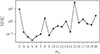 |
Fig. 3. Total MSE of the SDecGMCA reconstruction as a function of the number of sources ns. The MSE was computed with respect to the ground truth by combining the frequency and angular power spectra. |
The reconstructed spectra show (Fig. 4) that the optimal choice of ns is somewhat scale-dependent. At large frequency scales (low kν), ns = 5 suppresses excess power best, while the localized bump around kν ∼ 0.3 is more efficiently removed when ns = 6 is used. In the angular domain, the differences between the models are less pronounced at very large multipoles, where beam effects dominate, but at intermediate scales (ℓ ∼ 101 − 102), the reconstruction improves noticeably for ns = 7. This behavior reflects the fact that different astrophysical foregrounds and instrumental systematics dominate different scales, which requires varying degrees of model flexibility.
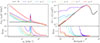 |
Fig. 4. Reconstructed HI frequency (left) and angular (right) power spectra obtained with SDecGMCA for different choices of the number of sources (ns, shown in different colors). The black line shows the input HI signal for reference, and the lower panels display the ratio of the reconstruction and the true signal. |
The most balanced reconstruction in both domains overall was obtained for ns = 5. Fig. 3 shows that the number of sources plays a role that is analogous to regularization. Too few sources (e.g., ns = 2 − 3) lack the flexibility needed to capture the complex spectral behavior of the foregrounds, causing residual contamination to leak into the HI signal. Too many sources (e.g., ns ≳ 10) risk overfitting, as the algorithm tends to fragment coherent astrophysical components into multiple modes, which reintroduces noise and residuals. This trade-off is clearly visible in the MSE curve, which rises again at high ns. The importance of carefully choosing the number of sources has also been emphasized in the HI extraction literature, where a range of BSS methods applied to different experimental configurations consistently highlighted this trade-off (e.g., Chapman et al. 2013; Mertens et al. 2018; Carucci et al. 2020, 2025; Hothi et al. 2021).
In summary, while SDecGMCA is capable of robustly recovering the HI power spectra, its performance remains sensitive to the choice of ns. A moderate number of sources (ns ≃ 5 − 7) provides the best compromise at all scales, although the precise optimum can vary depending on the kν or ℓ range of interest. A practical challenge arises when the method is applied to real data, where no ground truth is available and the optimal value of ns cannot be identified directly. In these cases, indirect diagnostics such as the eigenvalues of the covariance matrix of the signal, the stability of the recovered power spectra, or cross-correlations with external tracers are needed.
Another important set of hyperparameters in SDecGMCA are those associated with the thresholding procedure. We do not discuss them in detail here because they are more technical and beyond the scope of this work. In a follow-up study, however, we will show that replacing the current thresholding scheme with a structured convolutional neural network that acts as a learned wavelet-like multiscale representation (Bonjean et al. 2026) can effectively eliminate the dependence of the method on these hyperparameters.
5. Masking effect
Masking the bright peaks in the frequency profiles of individual lines of sight (Appendix B) helps to improve the HI reconstruction. These peaks correspond to bright HI sources and not to extragalactic point sources, which has already been studied by Matshawule et al. (2021). In particular, this masking of the peaks mitigates systematic offsets in the frequency power spectrum, such as the broadband bias at all scales reported by Spinelli et al. (2021) and also observed in our results. While SDecGMCA demonstrates an improved performance under these conditions, particularly in the challenging oscillating-beam case, regions of the sky remain in which the method fails to accurately reconstruct the underlying HI signal. A likely contributing factor is the inclusion of the Galactic plane and other extremely bright lines of sight in the input maps, which make the separation even more challenging.
In this section, we examine the effect of excluding or attenuating these bright-foreground regions on the quality of the HI signal reconstruction. Although directly applying a Galactic mask during component separation is currently incompatible with the SDecGMCA framework, we explored two indirect approaches: first, by post-processing the reconstructed HI signal to exclude lines of sight with problematic reconstruction (Sect. 5.1), and second, by artificially dimming the foreground amplitude in and around the Galactic plane to simulate the effect of a Galactic mask (Sect. 5.2).
5.1. Post-masking
To investigate the origin of the spurious peak in the frequency power spectrum and the excess power at low kν, we closely examined the reconstructed HI maps from all foreground removal methods. We observed that for a subset of lines of sight, there is coherent spectral structure as a function of frequency, which is indicative of leaked foregrounds. To identify which lines of sight contribute to the residuals, we computed the MSE between the reconstructed and true HI signal along each line of sight (MSElos). We then flagged the lines of sight with |⟨MSE⟩−MSElos|> σMSE, where ⟨ ⋅ ⟩ denotes the mean and σ the standard deviation over all lines of sight.
The resulting flagged lines of sight are illustrated in Fig. 5 as spectral profiles (brightness temperature versus frequency) and spatially on the sky. Visually, it is evident that these contaminated lines of sight are located along the Galactic plane, where foreground emission is particularly strong. To evaluate their effect on the reconstructed power spectra, we excluded the flagged regions when we computed the frequency and angular power spectra of the recovered HI maps. The results of this analysis are presented in Fig. 6.
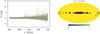 |
Fig. 5. Filtering lines of sight prior to computing the power spectrum of the reconstructed HI signal. Left: Brightness temperature of the reconstructed HI signal as a function of frequency for all flagged lines of sight that deviate from the expected spectral flatness. Right: Sky map showing the location of the flagged lines of sight, illustrating the regions excluded by the constructed mask. The percentage of lines of sight that are masked is indicated at the top of the map. |
This post-processing reduced the amplitude of the peak in the frequency power spectrum further, as shown in the left panel of Fig. 6. Moreover, the HI signal was recovered down to lower kν scales, which significantly improved the fidelity of the reconstruction. To ensure a fair comparison, we applied the same masking procedure to the outputs of the other methods, but found no significant improvement. This suggests that their performance degradation is introduced during foreground removal and exceeds what can be mitigated by post-processing.
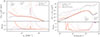 |
Fig. 6. Effect of post-processing masking on the HI signal reconstruction for the oscillating beam. Left: Frequency power spectrum of the reconstructed HI signal. The solid black curve shows the true HI signal plus noise, and the dotted red curve represents the SDecGMCA reconstruction before masking. The dashed red curve shows the result after excluding problematic lines of sight, which suppresses the spurious peak and improves recovery at lower kν. Other methods are shown in lighter transparent lines for comparison, with minimum improvement observed. Right: Same as the left panel, but for the angular power spectrum of the reconstructed HI signal. The top panel displays the reconstructed power spectra from different methods, and the bottom panel shows the ratio to the true signal. |
In addition, we applied the mask described in the previous subsection to the angular power spectrum. Masking the Galactic plane before spectrum estimation is a standard practice in the CMB literature (e.g., Bennett et al. 2003; Planck Collaboration XXV 2016), where regions of bright Galactic emission are excluded to reduce contamination and improve the robustness of the cosmological inference. The resulting angular power spectra, shown in the right panel of Fig. 6, demonstrate the clear benefits of this strategy. Excluding the Galactic plane significantly improves the reconstruction of the HI signal for all BSS methods. Among them, SDecGMCA benefits most and successfully recovering the HI power spectrum down to smaller multipoles compared to the case without post-processing masking.
5.2. Simulating a Galactic mask
Encouraged by the improvements observed when bright regions were excluded from the power spectrum computation, we next explored whether incorporating a masking strategy before applying the separation methods might yield similar or even stronger benefits. Since direct masking is not currently supported by SDecGMCA, we simulated this scenario by artificially dimming the foregrounds in and around the Galactic plane. This approach mimics an observational strategy that avoids highly contaminated regions of the sky and allowed us to evaluate the effect of bright Galactic structures on the reconstruction quality.
To test this idea in a controlled and continuous way, we applied a smooth Gaussian weighting function in Galactic latitude to the simulated foreground maps. The weights preserved the signal outside |b|> 15° and decreased gradually toward the plane, reaching 0.1 at b = 0°. Each frequency map was multiplied by this latitude-dependent weight, after which the maps were smoothed with the telescope beam and instrumental noise was added, following the same procedure as for the unmasked simulations. We then applied all foreground removal methods to these artificially dimmed maps using the Gaussian-oscillating beam. The reconstructed spectra are shown in Fig. 7. This mock masking improved the performance of all methods, nd the most significant gains were seen for PCA, FastICA, and SDecGMCA.
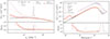 |
Fig. 7. Frequency (left) and angular (right) power spectra of the reconstructed HI signal obtained with different foreground removal methods, shown in various colors. All methods were applied to simulated maps with artificially dimmed foregrounds. These maps were convolved with a Gaussian-oscillating beam prior to signal reconstruction. |
In the frequency domain, the spurious peak persisted for PCA and FastICA, but was suppressed to below the 2% level for SDecGMCA. This confirms the result already reported by Matshawule et al. (2021), namely that the peak is primarily driven by lines of sight that are dominated by exceptionally bright foregrounds. Our findings therefore strengthen the case that excluding these regions prior to component separation can substantially improve the recovery of the cosmological signal.
In the angular domain, dimming the Galactic plane improves the performance of PCA, FastICA, and SDecGMCA alike by extending the multipole range over which the HI signal is accurately reconstructed. This result suggests that masking bright regions prior to foreground removal can be beneficial not only for SDecGMCA, but also for other BSS methods, in particular, for the angular power spectrum.
6. Conclusions
We assessed the performance of SDecGMCA, an extension of DecGMCA to spherical data that jointly perform source separation, for HI 21 cm intensity mapping under increasingly realistic beam conditions. We also compared our results to widely used and known foreground removal techniques, both model-fitting and BSS methods. Our main findings are summarized below.
-
Under the simplest Gaussian-degraded beam, all methods recovered the HI angular and frequency power spectra with an accuracy better than 10% for a broad range of scales, as expected given the preserved spectral smoothness of the foregrounds.
-
When the beam evolves smoothly with frequency, the performance of the methods diverges. Parametric fitting fails entirely, GMCA starts to degrade at intermediate scales in the angular (ℓ ∼ 40) and frequency (kν ∼ 0.2) power spectrum, and PCA, FastICA, and SDecGMCA maintain the accuracy over wider ranges in the angular (4 ≲ ℓ ≲ 200) and frequency (kν > 0.1) domains.
-
In the most realistic and challenging oscillating-beam case, the fitting approaches failed catastrophically, and only BSS methods remained viable. Of these, SDecGMCA achieved the most accurate reconstruction. It suppressed the spurious peak at kν ∼ 0.3 and recovered the angular spectrum at intermediate multipoles (20 < ℓ < 200). Nevertheless, beam inversion remains a fundamental limitation and produces unstable results beyond ℓ ∼ 200.
-
The number of sources ns is a critical hyperparameter for BSS methods. A moderate choice of ns ≃ 5 − 7 provides the best balance between underfitting and overfitting, and the precise optimum is scale dependent. This sensitivity highlights the need for robust data-driven strategies for setting ns in real observations, where no ground truth is available.
-
We further explored masking strategies. Post-processing by excluding foreground-contaminated lines of sight substantially reduced residual artifacts in SDecGMCA, including the suppression of the spurious peak and improved recovery at low multipoles. Simulating a Galactic mask by dimming the Galactic plane demonstrated that this masking improved the performance of PCA, FastICA, and especially SDecGMCA by extending the multipole range over which the HI signal can be reconstructed reliably.
Our results taken together highlight the promise and limitations of current approaches. Simple fitting methods are inadequate when realistic instrumental effects are introduced, while standard BSS techniques such as PCA, FastICA, and GMCA only partially cope with beam distortions. SDecGMCA stands out as a very promising option. It consistently performed in all scenarios we tested. Its dependence on the hyperparameters (particularly ns and the regularization scheme) and the intrinsic instability of the beam inversion remain major challenges, however.
Future work should focus on three directions: (i) incorporating masking strategies directly into the SDecGMCA framework, (ii) developing reliable diagnostics for setting hyperparameters from data, and (iii) refining the thresholding scheme (Bonjean et al. 2026). Even without these refinements, our results showed that SDecGMCA already delivers robust reconstructions on full-sky simulations without pre-masking. This establishes it as a particularly promising technique for the upcoming 21 cm intensity mapping surveys.
Acknowledgments
This work was funded by the TITAN ERA Chair project (contract no. 101086741) within the Horizon Europe Framework Program of the European Commission, the French Agence Nationale de la Recherche (ANR-22-CE31-0014-01 TOSCA) and the French Programme National de Cosmologie et Galaxies (PNCG project CIMES).
References
- Acharya, A., Mertens, F., Ciardi, B., et al. 2023, ArXiv e-prints [arXiv:2311.16633] [Google Scholar]
- Alonso, D., Ferreira, P. G., & Santos, M. G. 2014, MNRAS, 444, 3183 [NASA ADS] [CrossRef] [Google Scholar]
- Alonso, D., Bull, P., Ferreira, P. G., & Santos, M. G. 2015, MNRAS, 447, 400 [NASA ADS] [CrossRef] [Google Scholar]
- Amiri, M., Bandura, K., Chen, T., et al. 2023, ApJ, 947, 16 [NASA ADS] [CrossRef] [Google Scholar]
- Amiri, M., Bandura, K., Chakraborty, A., et al. 2024, ApJ, 963, 23 [Google Scholar]
- Anderson, C. J., Luciw, N. J., Li, Y. C., et al. 2018, MNRAS, 476, 3382 [NASA ADS] [CrossRef] [Google Scholar]
- Ansari, R., Campagne, J. E., Colom, P., et al. 2012, A&A, 540, A129 [NASA ADS] [CrossRef] [EDP Sciences] [Google Scholar]
- Asad, K. M. B., Girard, J. N., de Villiers, M., et al. 2021, MNRAS, 502, 2970 [CrossRef] [Google Scholar]
- Battye, R. A., Davies, R. D., & Weller, J. 2004, MNRAS, 355, 1339 [NASA ADS] [CrossRef] [Google Scholar]
- Battye, R. A., Browne, I. W. A., Dickinson, C., et al. 2013, MNRAS, 434, 1239 [NASA ADS] [CrossRef] [Google Scholar]
- Bennett, C. L., Smoot, G. F., Hinshaw, G., et al. 1992, ApJ, 396, L7 [NASA ADS] [CrossRef] [Google Scholar]
- Bennett, C. L., Halpern, M., Hinshaw, G., et al. 2003, ApJS, 148, 1 [Google Scholar]
- Bigot-Sazy, M. A., Dickinson, C., Battye, R. A., et al. 2015, MNRAS, 454, 3240 [NASA ADS] [CrossRef] [Google Scholar]
- Bobin, J., Starck, J.-L., Fadili, J., & Moudden, Y. 2007, IEEE Trans. Image Process., 16, 2662 [NASA ADS] [CrossRef] [Google Scholar]
- Bobin, J., Sureau, F., Starck, J. L., Rassat, A., & Paykari, P. 2014, A&A, 563, A105 [NASA ADS] [CrossRef] [EDP Sciences] [Google Scholar]
- Bobin, J., Sureau, F., & Starck, J. L. 2016, A&A, 591, A50 [NASA ADS] [CrossRef] [EDP Sciences] [Google Scholar]
- Bonjean, V., Gkogkou, A., Starck, J. L., & Tsakalides, P. 2026, A&A, in press, https://doi.org/10.1051/0004-6361/202556228 [Google Scholar]
- Bull, P., Ferreira, P. G., Patel, P., & Santos, M. G. 2015, ApJ, 803, 21 [NASA ADS] [CrossRef] [Google Scholar]
- Carloni Gertosio, R., & Bobin, J. 2021, Digital Signal Processing, 110, 102946 [Google Scholar]
- Carucci, I. P., Irfan, M. O., & Bobin, J. 2020, MNRAS, 499, 304 [NASA ADS] [CrossRef] [Google Scholar]
- Carucci, I. P., Bernal, J. L., Cunnington, S., et al. 2025, A&A, 703, A222 [NASA ADS] [CrossRef] [EDP Sciences] [Google Scholar]
- Chang, T.-C., Pen, U.-L., Peterson, J. B., & McDonald, P. 2008, Phys. Rev. Lett., 100, 091303 [NASA ADS] [CrossRef] [Google Scholar]
- Chapman, E., Abdalla, F. B., Harker, G., et al. 2012, MNRAS, 423, 2518 [NASA ADS] [CrossRef] [Google Scholar]
- Chapman, E., Abdalla, F. B., Bobin, J., et al. 2013, MNRAS, 429, 165 [CrossRef] [Google Scholar]
- Chen, T., Bianco, M., Tolley, E., et al. 2024, MNRAS, 532, 2615 [Google Scholar]
- Chen, Z., Cunnington, S., Pourtsidou, A., et al. 2025, ApJS, 279, 19 [Google Scholar]
- Crighton, N. H. M., Murphy, M. T., Prochaska, J. X., et al. 2015, MNRAS, 452, 217 [Google Scholar]
- Cunnington, S., Wolz, L., Pourtsidou, A., & Bacon, D. 2019, MNRAS, 488, 5452 [Google Scholar]
- Cunnington, S., Irfan, M. O., Carucci, I. P., Pourtsidou, A., & Bobin, J. 2021, MNRAS, 504, 208 [NASA ADS] [CrossRef] [Google Scholar]
- Cunnington, S., Wolz, L., Bull, P., et al. 2023, MNRAS, 523, 2453 [Google Scholar]
- Delabrouille, J., Betoule, M., Melin, J. B., et al. 2013, A&A, 553, A96 [NASA ADS] [CrossRef] [EDP Sciences] [Google Scholar]
- Draine, B. T. 2011, Physics of the Interstellar and Intergalactic Medium (Princeton: Princeton University Press) [Google Scholar]
- Fernández, X., Gim, H. B., van Gorkom, J. H., et al. 2016, ApJ, 824, L1 [Google Scholar]
- Fonseca, J., & Liguori, M. 2021, MNRAS, 504, 267 [Google Scholar]
- Furlanetto, S. R., Oh, S. P., & Briggs, F. H. 2006, Phys. Rep., 433, 181 [Google Scholar]
- Godinaud, L., Acero, F., Decourchelle, A., & Ballet, J. 2023, A&A, 680, A80 [NASA ADS] [CrossRef] [EDP Sciences] [Google Scholar]
- Gogate, A. R., Verheijen, M. A. W., Deshev, B. Z., et al. 2020, MNRAS, 496, 3531 [NASA ADS] [CrossRef] [Google Scholar]
- Górski, K. M., Hivon, E., Banday, A. J., et al. 2005, ApJ, 622, 759 [Google Scholar]
- Hothi, I., Chapman, E., Pritchard, J. R., et al. 2021, MNRAS, 500, 2264 [Google Scholar]
- Hyvarinen, A. 1999, IEEE Trans. Neural Netw., 10, 626 [Google Scholar]
- Jelić, V., Zaroubi, S., Labropoulos, P., et al. 2008, MNRAS, 389, 1319 [CrossRef] [Google Scholar]
- Jiang, M., Bobin, J., & Starck, J. L. 2017, ArXiv e-prints [arXiv:1703.02650] [Google Scholar]
- Kovetz, E. D., Viero, M. P., Lidz, A., et al. 2017, ArXiv e-prints [arXiv:1709.09066] [Google Scholar]
- Li, L.-C., Staveley-Smith, L., & Rhee, J. 2021, RAA, 21, 030 [Google Scholar]
- Liu, A., & Tegmark, M. 2011, Phys. Rev. D, 83, 103006 [NASA ADS] [CrossRef] [Google Scholar]
- Maćkiewicz, A., & Ratajczak, W. 1993, Comput. Geosci., 19, 303 [CrossRef] [Google Scholar]
- Makinen, T. L., Lancaster, L., Villaescusa-Navarro, F., et al. 2021, J. Cosmol. Astropart. Phys., 2021, 081 [Google Scholar]
- Marins, A., Abdalla, F. B., Fornazier, K. S. F., et al. 2022, ArXiv e-prints [arXiv:2209.11701] [Google Scholar]
- Martin, A. M., Giovanelli, R., Haynes, M. P., & Guzzo, L. 2012, ApJ, 750, 38 [Google Scholar]
- Masui, K. W., Switzer, E. R., Banavar, N., et al. 2013, ApJ, 763, L20 [Google Scholar]
- Matshawule, S. D., Spinelli, M., Santos, M. G., & Ngobese, S. 2021, MNRAS, 506, 5075 [Google Scholar]
- Mazumder, A., Wolz, L., Chen, Z., et al. 2025, MNRAS, 541, 476 [Google Scholar]
- MeerKLASS Collaboration (Chatterjee, S., et al.) 2025, MNRAS, 537, 3632 [Google Scholar]
- Mertens, F. G., Ghosh, A., & Koopmans, L. V. E. 2018, MNRAS, 478, 3640 [NASA ADS] [Google Scholar]
- Miville-Deschênes, M. A., Ysard, N., Lavabre, A., et al. 2008, A&A, 490, 1093 [NASA ADS] [CrossRef] [EDP Sciences] [Google Scholar]
- Ni, S., Li, Y., Gao, L.-Y., & Zhang, X. 2022, ApJ, 934, 83 [Google Scholar]
- Ni, S., Qiu, Y., Chen, Y., et al. 2025, ApJ, 990, 122 [Google Scholar]
- Olivari, L. C., Remazeilles, M., & Dickinson, C. 2016, MNRAS, 456, 2749 [NASA ADS] [CrossRef] [Google Scholar]
- Paul, S., Santos, M. G., Chen, Z., & Wolz, L. 2023, ArXiv e-prints [arXiv:2301.11943] [Google Scholar]
- Peterson, J. B., Aleksan, R., Ansari, R., et al. 2009, Astro2010: The Astronomy and Astrophysics Decadal Survey, Science White Papers, 234 [Google Scholar]
- Planck Collaboration XXV. 2016, A&A, 594, A25 [NASA ADS] [CrossRef] [EDP Sciences] [Google Scholar]
- Pritchard, J. R., & Loeb, A. 2012, Rep. Prog. Phys., 75, 086901 [NASA ADS] [CrossRef] [Google Scholar]
- Remazeilles, M., Dickinson, C., Banday, A. J., Bigot-Sazy, M. A., & Ghosh, T. 2015, MNRAS, 451, 4311 [NASA ADS] [CrossRef] [Google Scholar]
- Santos, M. G., Cooray, A., & Knox, L. 2005, ApJ, 625, 575 [NASA ADS] [CrossRef] [Google Scholar]
- Santos, M., Bull, P., Alonso, D., et al. 2015, Advancing Astrophysics with the Square Kilometre Array (AASKA14), 19 [Google Scholar]
- Shaw, J. R., Sigurdson, K., Sitwell, M., Stebbins, A., & Pen, U.-L. 2015, Phys. Rev. D, 91, 083514 [Google Scholar]
- Shi, F., Chang, H., Zhang, L., et al. 2024, Phys. Rev. D, 109, 063509 [Google Scholar]
- Soares, P. S., Watkinson, C. A., Cunnington, S., & Pourtsidou, A. 2022, MNRAS, 510, 5872 [Google Scholar]
- Spinelli, M., Carucci, I. P., Cunnington, S., et al. 2021, MNRAS, 509, 2048 [NASA ADS] [CrossRef] [Google Scholar]
- Starck, J.-L., Fadili, J., & Murtagh, F. 2007, IEEE Trans. Image Process., 16, 297 [Google Scholar]
- Starck, J., Murtagh, F., & Fadili, J. 2016, Sparse Image and Signal Processing: Wavelets and Related Geometric Multiscale Analysis, 2nd edn. (Cambridge: Cambridge University Press) [Google Scholar]
- Switzer, E. R., Masui, K. W., Bandura, K., et al. 2013, MNRAS, 434, L46 [NASA ADS] [CrossRef] [Google Scholar]
- Thorne, B., Dunkley, J., Alonso, D., & Næss, S. 2017, MNRAS, 469, 2821 [Google Scholar]
- Tramonte, D., & Ma, Y.-Z. 2020, MNRAS, 498, 5916 [Google Scholar]
- Villaescusa-Navarro, F., Anglés-Alcázar, D., Genel, S., et al. 2021, ApJ, 915, 71 [NASA ADS] [CrossRef] [Google Scholar]
- Wolz, L., Abdalla, F. B., Blake, C., et al. 2014, MNRAS, 441, 3271 [NASA ADS] [CrossRef] [Google Scholar]
- Wolz, L., Blake, C., Abdalla, F. B., et al. 2017, MNRAS, 464, 4938 [NASA ADS] [CrossRef] [Google Scholar]
- Wolz, L., Pourtsidou, A., Masui, K. W., et al. 2022, MNRAS, 510, 3495 [NASA ADS] [CrossRef] [Google Scholar]
- Zhang, L., Bunn, E. F., Karakci, A., et al. 2016, ApJS, 222, 3 [Google Scholar]
- Zonca, A., Thorne, B., Krachmalnicoff, N., & Borrill, J. 2021, J. Open Source Softw., 6, 3783 [NASA ADS] [CrossRef] [Google Scholar]
Appendix A: Complementary diagnostics
We present additional quantitative diagnostics for the case of the most challenging beam configuration, the oscillating beam, that further assess the performance of the foreground removal methods in reconstructing the cosmological HI signal. These metrics provide complementary insight beyond the power-spectrum analysis discussed in Sect. 4.
Pearson correlation coefficient per map
As a first additional diagnostic, we compute the Pearson correlation coefficient between the reconstructed and true HI maps at each frequency channel. This coefficient quantifies the degree of linear correlation between the spatial fluctuations of the reconstructed (Trec) and input (Ttrue) HI brightness temperature maps:
 (A.1)
(A.1)
where the summation runs over all sky pixels i, from 1 to Npix. Values of r(ν) close to unity indicate a faithful recovery of the spatial HI structure at frequency ν, whereas lower values point to residual foreground contamination or signal loss. As shown in Fig. A.1, SDecGMCA consistently achieves the highest correlation across frequencies, demonstrating superior reconstruction fidelity compared to the other methods.
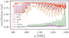 |
Fig. A.1. Pearson correlation coefficient between the reconstructed and true HI maps as a function of frequency. Values close to unity indicate an accurate recovery of the true HI structure, while lower values reveal residual foreground contamination or signal loss. |
Variance of the fractional Cℓ difference
To complement the map-based correlation analysis, we evaluate the variance of the fractional residual difference in the angular power spectrum,
 (A.2)
(A.2)
averaged over frequency channels. This quantity characterizes the relative deviation of the reconstructed HI power from the true one at each multipole. We then compute the variance of Rℓ across all frequency channels as
 (A.3)
(A.3)
which provides a quantitative measure of the stability and consistency of each method across scales. Lower values of σRℓ2 indicate more uniform performance and reduced scale-dependent bias. As illustrated in Fig. A.2, SDecGMCA exhibits the smallest variance at intermediate multipoles (10 ≲ ℓ ≲ 200), confirming its robustness and stability in reconstructing the HI signal.
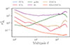 |
Fig. A.2. Variance of the fractional Cℓ difference as a function of multipole. Lower values correspond to more uniform and consistent performance. |
Appendix B: Masking in frequency space
In this appendix we describe in detail the pre-processing step used to identify and mask sharp peaks in the temperature profiles, which can bias foreground removal. The procedure begins by fitting a sixth-order polynomial along each line of sight (LOS) in the total observed temperature maps (see top panel of Fig. B.1). Subtracting this polynomial from the original data flattens the spectra, as illustrated in Fig. B.2. To identify and exclude bright peaks, we apply sigma clipping with a threshold of 5σ to the flattened residuals. Pixels flagged as outliers (stars in bottom panel of Fig. B.1) are masked.
A second polynomial fit is then performed on the original total temperature profile, this time excluding the masked pixels. Subtracting this refined baseline yields a more accurate estimate and avoids bias from outliers. Figure B.2 compares the results of baseline subtraction with and without masking. The blue curve shows the flattened signal when all pixels are included, while the orange curve demonstrates the improved baseline removal obtained after excluding bright outliers.
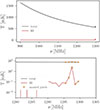 |
Fig. B.1. Temperature profile for a single line of sight. Top: Total observed brightness temperature T(ν) (black) and the underlying HI signal along the same LOS (red). Bottom: Zoom on the frequency range containing the prominent peak (note the logarithmic T scale). Star symbols mark the channels flagged by our sigma-clipping criterion and replaced by the second-pass polynomial baseline (Appendix B). This example corresponds to the line of sight hosting the brightest HI source in the simulation and illustrates the masking procedure. |
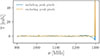 |
Fig. B.2. Flattened signal after baseline subtraction. The blue curve shows the result when all pixels are included in the polynomial fitting, while the orange curve shows the improved baseline obtained when bright outlier pixels are masked and excluded from the second fit. |
Finally, in the pre-processing strategy used throughout Sect. 4.1, we replaced the masked pixel values with the corresponding baseline values. This smoothing procedure is illustrated in Fig. B.3, where the black line shows the original total signal and the red line shows the smoothed result. This masking was applied consistently to all input temperature maps prior to running either the fitting-based or BSS-based foreground-removal methods, and it substantially improved the identification of foreground-dominated channels, leading to a more accurate HI reconstruction.
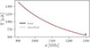 |
Fig. B.3. Temperature profile along a single LOS. The black line shows the original total signal, while the red line shows the smoothed signal obtained after applying the masking procedure described in Appendix B. |
All Tables
All Figures
|
Fig. 1. Angular power spectrum of the reconstructed HI 21 cm signal using different methods, each represented by a distinct color. The bottom panel displays the ratio of the reconstructed to the true HI power spectrum for each method. From left to right, the panels correspond to different beam models: Gaussian degraded, Gaussian evolving, and Gaussian oscillating. |
| In the text | |
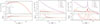 |
Fig. 2. Equivalent to Fig. 1, but showing the frequency power spectrum. |
| In the text | |
|
Fig. 3. Total MSE of the SDecGMCA reconstruction as a function of the number of sources ns. The MSE was computed with respect to the ground truth by combining the frequency and angular power spectra. |
| In the text | |
|
Fig. 4. Reconstructed HI frequency (left) and angular (right) power spectra obtained with SDecGMCA for different choices of the number of sources (ns, shown in different colors). The black line shows the input HI signal for reference, and the lower panels display the ratio of the reconstruction and the true signal. |
| In the text | |
|
Fig. 5. Filtering lines of sight prior to computing the power spectrum of the reconstructed HI signal. Left: Brightness temperature of the reconstructed HI signal as a function of frequency for all flagged lines of sight that deviate from the expected spectral flatness. Right: Sky map showing the location of the flagged lines of sight, illustrating the regions excluded by the constructed mask. The percentage of lines of sight that are masked is indicated at the top of the map. |
| In the text | |
|
Fig. 6. Effect of post-processing masking on the HI signal reconstruction for the oscillating beam. Left: Frequency power spectrum of the reconstructed HI signal. The solid black curve shows the true HI signal plus noise, and the dotted red curve represents the SDecGMCA reconstruction before masking. The dashed red curve shows the result after excluding problematic lines of sight, which suppresses the spurious peak and improves recovery at lower kν. Other methods are shown in lighter transparent lines for comparison, with minimum improvement observed. Right: Same as the left panel, but for the angular power spectrum of the reconstructed HI signal. The top panel displays the reconstructed power spectra from different methods, and the bottom panel shows the ratio to the true signal. |
| In the text | |
|
Fig. 7. Frequency (left) and angular (right) power spectra of the reconstructed HI signal obtained with different foreground removal methods, shown in various colors. All methods were applied to simulated maps with artificially dimmed foregrounds. These maps were convolved with a Gaussian-oscillating beam prior to signal reconstruction. |
| In the text | |
|
Fig. A.1. Pearson correlation coefficient between the reconstructed and true HI maps as a function of frequency. Values close to unity indicate an accurate recovery of the true HI structure, while lower values reveal residual foreground contamination or signal loss. |
| In the text | |
|
Fig. A.2. Variance of the fractional Cℓ difference as a function of multipole. Lower values correspond to more uniform and consistent performance. |
| In the text | |
|
Fig. B.1. Temperature profile for a single line of sight. Top: Total observed brightness temperature T(ν) (black) and the underlying HI signal along the same LOS (red). Bottom: Zoom on the frequency range containing the prominent peak (note the logarithmic T scale). Star symbols mark the channels flagged by our sigma-clipping criterion and replaced by the second-pass polynomial baseline (Appendix B). This example corresponds to the line of sight hosting the brightest HI source in the simulation and illustrates the masking procedure. |
| In the text | |
|
Fig. B.2. Flattened signal after baseline subtraction. The blue curve shows the result when all pixels are included in the polynomial fitting, while the orange curve shows the improved baseline obtained when bright outlier pixels are masked and excluded from the second fit. |
| In the text | |
|
Fig. B.3. Temperature profile along a single LOS. The black line shows the original total signal, while the red line shows the smoothed signal obtained after applying the masking procedure described in Appendix B. |
| In the text | |
Current usage metrics show cumulative count of Article Views (full-text article views including HTML views, PDF and ePub downloads, according to the available data) and Abstracts Views on Vision4Press platform.
Data correspond to usage on the plateform after 2015. The current usage metrics is available 48-96 hours after online publication and is updated daily on week days.
Initial download of the metrics may take a while.