| Issue |
A&A
Volume 706, February 2026
|
|
|---|---|---|
| Article Number | A169 | |
| Number of page(s) | 20 | |
| Section | Stellar structure and evolution | |
| DOI | https://doi.org/10.1051/0004-6361/202557572 | |
| Published online | 09 February 2026 | |
The demographics of core-collapse supernovae
The role of binary evolution and interaction with the circumstellar medium
1
Argelander Institut für Astronomie Auf dem Hügel 71 DE-53121 Bonn, Germany
2
Max-Planck-Institut für Radioastronomie Auf dem Hügel 69 DE-53121 Bonn, Germany
3
Department of Particle Physics and Astrophysics, Weizmann Institute of Science 234 Herzl Street IL-7610001 Rehovot, Israel
★ Corresponding author: This email address is being protected from spambots. You need JavaScript enabled to view it.
Received:
6
October
2025
Accepted:
2
December
2025
Abstract
Context. The observational properties of core-collapse supernovae are shaped by the envelopes of their progenitors. In massive binary systems, mass-transfer drastically alters the pre-supernova structures compared to single stars, which leads to a diversity in supernova explosions.
Aims. We computed the distribution of core-collapse supernova properties based on comprehensive detailed grids of single and binary stellar evolution models.
Methods. We conducted a grid-based population synthesis to produce a synthetic population of core-collapse supernovae and compared it to observed supernova samples. To do this, we applied various explodability and merger criteria to our models. In line with earlier results, we identified interacting supernova progenitors as those stars that undergo core collapse during or shortly after a Roche-lobe overflow phase.
Results. With an interacting binary fraction of 68%, our models predict that two-thirds of all core-collapse supernovae are Type IIP/L and one-third are Type Ibc. This agrees with recent volume-limited supernova surveys. We find that 76% of the Type Ibc supernova progenitors took part in a previous binary mass transfer (mostly as a mass donor), but 63% of the Type IIP/L supernova progenitors did this as well (mostly as mass gainers). This yields a much broader envelope mass distribution than expected from single stars. Mass-transfer-induced interacting supernovae make up ∼5% of all core-collapse supernovae, which is close to the observed fractions of Type IIn and Type Ibn supernovae. When a disk or toroidal geometry of the circumstellar medium is assumed for Type IIn supernovae, our models predict a bimodal distribution of the radiated energies that is similar to the distribution deduced from observations.
Conclusions. While we found the effect of binary evolution on the relative number of Type Ibc and Type IIP/L supernovae to be moderate, it leads to lower average ejecta masses in Type Ibc and Type IIb supernovae and can lead to higher pre-supernova masses in Type IIP/L supernovae than in single stars. Binary models are also able to reproduce the number and properties of interacting supernovae.
Key words: binaries: general / circumstellar matter / stars: evolution / stars: massive / stars: mass-loss / supernovae: general
© The Authors 2026
 Open Access article, published by EDP Sciences, under the terms of the Creative Commons Attribution License (https://creativecommons.org/licenses/by/4.0), which permits unrestricted use, distribution, and reproduction in any medium, provided the original work is properly cited.
This article is published in open access under the Subscribe to Open model. This email address is being protected from spambots. You need JavaScript enabled to view it. to support open access publication.
1. Introduction
Core-collapse supernovae mark the end of the life of stars that were initially more massive than Mi ≳ 9 M⊙ as their iron cores collapse and the released energy drives an explosion. These are among the most energetic events in the Universe and play a crucial role in enriching their host galaxies with metals and triggering subsequent episodes of star formation (McKee & Ostriker 1977; Mac Low & Klessen 2004; Mac Low et al. 2005; Nomoto et al. 2006).
Supernovae are classified observationally based on the presence of hydrogen in their spectra (see Gal-Yam 2017, for a review). H-rich events are labeled Type IIP or Type IIL, depending on the light curve, while stars whose progenitors were partially or fully stripped of the H-rich envelope give rise to Type IIb and Type Ibc supernovae, respectively (Young 2004; Dessart et al. 2011, 2024). All stripped-envelope supernovae provide a testbed for massive star evolution models. As single-star models underpredict their observed rates, several authors proposed binary evolution as a key formation channel (Eldridge et al. 2008; Smartt 2009; Smith et al. 2011; Eldridge et al. 2013).
Binary mass transfer is understood to play a dominant role in shaping the evolution and final fate of massive stars (Sana et al. 2012; Langer 2012). Donor stars in close binaries can be efficiently stripped of most if not all of their H-rich envelopes and produce H-poor or even He-poor supernovae (e.g., Podsiadlowski et al. 1992; Wellstein & Langer 1999; Yoon et al. 2010, 2017; Claeys et al. 2011; Sravan et al. 2019). Mass transfer also alters the structure and explosion timing of mass donors and mass gainers compared to single stars (Wellstein et al. 2001; Zapartas et al. 2017; Eldridge et al. 2017; Laplace et al. 2021).
Previously, the progenitors of Type Ibc supernovae were considered to be massive H-free Wolf-Rayet stars (e.g., Georgy et al. 2009; Groh et al. 2013). The current consensus has instead shifted to include progenitors that underwent binary-induced mass loss (Woosley et al. 1995; Wellstein & Langer 1999; Yoon et al. 2010, 2017), especially in light of transients with low-mass progenitors such as iPTF13bvn (Bersten et al. 2014; Fremling et al. 2014; Kuncarayakti et al. 2015; Yoon et al. 2017).
Some supernovae show strong observational signatures of an interaction with the surrounding circumstellar medium (CSM), implying significant mass-loss in the final stages before explosion (Smith 2017). These transients are categorized based on the composition of the narrow emission lines: H rich (Type IIn, Schlegel 1990), H poor, and He rich (Type Ibn; Pastorello et al. 2008), and H poor and He poor (Type Icn; Gal-Yam et al. 2022). Recent transient surveys such as the Asteroid Terrestrial-impact Last Alert System (ATLAS, Tonry et al. 2018), the All Sky Automated Survey for SuperNovae (ASAS-SN, Shappee et al. 2014), the Palomar Transient Factory (PTF, Law et al. 2009) and its successor surveys such as the Zwicky Transient Facility (ZTF, Bellm et al. 2019) have uncovered a larger number of these events, which are substantially diverse (e.g., Hiramatsu et al. 2024). One of the main avenues of research is to connect the progenitor stars and their evolution with these observed supernovae.
Models for interacting supernovae fall into two broad categories. One category attributes the mass loss to single-star-related mechanisms that take place just before core collapse, such as eruptions in Luminous Blue Variables (LBVs) or instabilities in the envelope or core (Woosley et al. 1980; Quataert & Shiode 2012; Smith & Arnett 2014; Woosley & Heger 2015; Fuller 2017; Wu & Fuller 2021; Schneider et al. 2025a). The other scenario involves inefficient mass-transfer in binary systems that occurs at late evolutionary stages (Ouchi & Maeda 2017; Matsuoka & Sawada 2024; Ercolino et al. 2024 for the H-rich transients and Wu & Fuller 2022; Ercolino et al. 2025 for the H-poor transients).
We present a grid-based binary population synthesis study informed by a comprehensive set of detailed stellar and binary evolution models (Jin et al. 2025) to predict the relative rates and progenitor properties of various core-collapse supernova types. Building on our earlier works on interacting supernovae (Ercolino et al. 2024 for Type IIn supernovae, hereafter EJLD24, and Ercolino et al. 2025 for Type Ibn supernovae, hereafter EJLD25), we provide quantitative estimates of the populations of interacting supernovae.
We introduce our models and assumptions in Sect. 2 and discuss our results in Sect. 3. We compare our results with the observations in Sect. 4 before we conclude in Sect. 5.
2. Method
2.1. Stellar evolutionary models
We considered stellar evolution models from the Bonn-GAL grid (Jin et al. 2025) computed with the code MESA (r10389, Paxton et al. 2011, 2013, 2015, 2018), which includes differentially rotating single- and binary-evolution models at solar metallicity. Since these models are only evolved until the end of core C-burning, we additionally computed two single-star grids that reached core collapse, which enabled us to estimate the explosion properties for progenitors across the parameter space (see Sect 2.2.3). The details of the grids are listed in Table 1.
List of stellar evolutionary model grids
In the following, we only discuss the relevant physics and assumptions in the context of this work. We refer to Jin et al. (2024) and Jin et al. (2025) for a complete description of the stellar evolutionary models. A discussion of the effects of the physics used in the stellar models on our results can be found in Appendix A.1.
2.1.1. Stellar physics
Stars were initialized with an initial rotational velocity of roughly 20% of the breakup rotation (corresponding to the first peak in the observed distribution in Dufton et al. 2013, roughly 150 km s−1). The Bonn-GAL grid adopted the stern nuclear network (Heger et al. 2000; Jin et al. 2024, 2025) and the simulations were terminated at the depletion of C in the core. Lower-mass models were terminated when they developed into asymptotic giant branch stars.
The models use the wind mass-loss recipe of Pauli et al. (2022), which is built upon that of Brott et al. (2011). For hot H-rich stars (X > 0.7), the wind mass-loss rate was taken from Vink et al. (2001), while for cool H-rich stars, the maximum between the rates of Vink et al. (2001) and Nieuwenhuijzen & de Jager (1990) was adopted. For H-poor stars (X < 0.4), the Wolf-Rayet wind mass-loss rates from Nugis & Lamers (2000) were adopted until the star became H free, at which point, the rates from Yoon (2017) were implemented. Rotationally enhanced mass loss was also accounted for following Heger et al. (2000), which resulted in a boost of a factor of (1 − vrot/vcrit)−0.43, where the critical velocity is also a function of the Eddington factor.
Convective regions were treated via the mixing-length theory with αMLT = 1.5. Stellar models show subsurface convectively unstable regions in which the envelope is locally super-Eddington, and they result in inflated envelopes (Sanyal et al. 2015) that give rise to numerical instabilities in extended stars with a high luminosity-to-mass ratio L/M. Therefore, the Bonn-GAL models additionally include MLT++ (Paxton et al. 2013) after the end of the main sequence to reduce the superadiabaticity of the outermost layers. This treatment also results in systematically smaller radii in affected stars and thus affects the onset of mass-transfer episodes in partially stripped stars (see Appendix A.1.2). The convective boundaries were determined via the Ledoux criterion, and semiconvection was included with an efficiency parameter αsc = 1 (Schootemeijer et al. 2019).
2.1.2. Binary physics
Binary models were initialized in a circular orbit, and the two stars were computed simultaneously until one of the two reached an advanced evolutionary stage (Jin et al. 2025). When one star was expected to reach core collapse, the binary was broken up and the computation of the companion was continued until it also reached the end of its life. When it was otherwise expected to become a white dwarf (WD), it was set to a point mass, and the companion was seamlessly evolved in the binary. When there were convergence issues, the binary simulation was terminated.
When stars evolve in binaries, they can undergo one or more phases of mass transfer via Roche-lobe overflow (RLOF), which is implemented via the contact scheme during the main sequence (Paxton et al. 2013) and Kolb & Ritter (1990) after one star evolves out of the main-sequence. We assumed rotation-limited accretion on the companion star and that the lost material carries away the same specific angular momentum as the accretor. This prevented the accretors from gaining significant amounts of mass, unless they were in tight binaries (Jin et al. 2025).
Mass transfer can turn unstable, which might lead the system into a common-envelope phase (Paczynski et al. 1976) in which the companion star in-spirals within the envelope of the donor star. We assumed that this phase resulted in the merger of the two stars. We made an exception for unstable Case C RLOF because the in-spiral timescale might be comparable to or even exceed the remaining time before core collapse, allowing the donor to explode before the merger occurs (see EJLD24).
Several criteria were used to identify binary models that undergo unstable mass transfer and function as termination conditions (Jin et al. 2025), encompassing L2-overflow during the overcontact phase, mass transfer initiated at the zero-age main sequence (ZAMS), the occurrence of Darwin instability (Darwin 1879), inverse mass transfer, and models with qi < 0.7, where the mass transfer rates exceed 0.1 M⊙ yr−1. The models that prematurely terminated during Case A or Case B mass transfer were assumed to merge. This ensemble of choices defines the hard-coded merger criterion, which outlines the baseline for the number of systems that result in mergers.
2.2. Population synthesis
We estimated the population properties of supernova progenitors using a grid-based population synthesis of the stellar evolutionary models, assigning statistical weights to each model in the grid. This was motivated by the widespread presence of sharp transitions in the parameter space, which disfavor the adoption of interpolation-based Monte Carlo methods.
We describe our assumptions on the birth probabilities of each model (Sect. 2.2.1), and on the inferred properties of the models beyond the stellar-evolution calculations, namely the evolution of mergers (Sect. 2.2.2), the explodability of the models (Sect. 2.2.3), and the evolution of the binary system after the first explosion (Sect. 2.2.4). We discuss the effect of these assumptions in Appendix A.2.
2.2.1. Birth probabilities
The single-star and binary grids covered an extensive parameter space for the initial mass M1, i, period Pi, and mass ratios qi (see Table 1). We adopted a power-law distribution for Mi, that is, the initial mass function (IMF; Salpeter 1955; Kroupa et al. 2001) and for qi and Pi, and we wrote the overall probability density function of a system that was born as a binary (dnB) or as a single star (dnS) as
 (1)
(1)
with fB the birth-binary fraction, and fS = 1 − fB the birth single-star fraction. The power-law exponents were taken as α = −2.35 (Salpeter 1955; for binaries, we used the initial mass of the more massive component), while the most recent literature suggested β ∈ [ − 0.1, −0.2] (Almeida et al. 2017; Sana et al. 2025) and γ = −0.10 ± 0.58 (Sana et al. 2012). Considering the relatively high uncertainty of these last two indices, we adopted a flat distribution with γ = β = 0. In Appendix A.2.2 we elaborate on the effect of employing different distribution powers on our results.
Each binary model in the grid (with initial conditions log M1, i, log Pi, and qi) represented the systems within a short interval from its initial conditions. We took this interval as δ/2, with δ = 0.05 being the grid resolution in log M1, i, log Pi, and qi. Statistical weights were assigned by integrating the probability density (Eq. (1)) over the discrete volume elements. For single stars, we proceeded analogously (where only the initial mass changes between models), but included a finer grid in mass by interpolating by the initial model mass.
We sampled our single-star and binary models assuming a mass-independent birth binary fraction of stellar systems of fB = 75% (Sana et al. 20121). Translating these into the numbers of stars yields that about 14.3% of them are born as single-stars and 85.7% are in a binary system. Our widest binary models did not undergo any mass transfer, and we therefore defined an empirical interacting-binary fraction fBMT as the fraction of systems at birth that underwent mass-transfer. Assuming a Salpeter IMF, flat-log Pi and flat-qi distributions, we obtained fBMT = 67.8%, while for effectively single-star systems (which include wide binaries that did not undergo mass transfer), the fraction is fSeff = fS + (fB − fBMT) = 32.2%. This translates into 22.5% of stars that are born in single- or effectively single-star systems, while 77.5% of the stars undergo mass transfer with a companion.
2.2.2. Mergers and their evolution
The evolution of a binary system after the onset of unstable mass transfer was the topic of many recent studies (Ivanova et al. 2020; Schneider et al. 2025b) with a focus on multidimensional simulations (Lau et al. 2022, 2025; Gagnier & Pejcha 2023, 2025) and one-dimensional approximations (Marchant et al. 2021; Hirai & Mandel 2022; Bronner et al. 2024). The debate over the physics of the common-envelope phase is still ungoing, but these studies suggested that most of the systems such as those we labeled as undergoing unstable mass transfer will merge.
We assumed that unstable Case A or Case B mass transfer between two nondegenerate stars always leads to a merger (see Sect. 2.2.4 for the case with a degenerate companion). The evolution of the merger product was investigated in previous studies (Menon & Heger 2017; Menon et al. 2024; Schneider et al. 2024), but it depends on the different adopted physical assumptions. We simplified the treatment of these stars and separated them according to whether they formed during Case A RLOF, Case B RLOF, or inverse mass transfer.
For Case A merger products, we assumed complete rejuvenation, such that the merger product truly resembled a single star of the same total mass(which is justified considering the high semiconvection adopted, Braun & Langer 1995). Its evolution was therefore mapped to the single-star model with the same mass. These stars might show strong magnetic fields (Schneider et al. 2019), however, which are not included in the calculations. We assumed that mergers in which at least one star developed a H-free core (i.e. Case B and inverse mass transfer) form a star in which the H-free core and the envelope are the sum of those from the two progenitor stars. The final properties of these models at core collapse were evaluated by mapping our merger models (defined by their initial mass and the relative amount of mass accreted) to the models studied by Schneider et al. (2024).
We explored additional criteria to identify models undergoing unstable mass transfer that then merge (as compared to the hard-coded criteria in Sect. 2.1.2) by post-processing the models in the grid. This allowed us to discuss the effects of these criteria on the population of supernovae. We included two broad categories of merger criteria that either defined the mass-transfer stability via the successful ejection of unaccreted material via radiation (which we will refer to as the “Energy” criterion, Marchant 2017) or the presence of outflows from the outer Lagrangian point (which we refer to as the OLOF criterion; Pavlovskii & Ivanova 2015). These two criteria flag a model as undergoing unstable mass transfer even when the respective condition is met for a short time. We therefore included a delayed energy criterion (Pauli 2020) and a delayed OLOF criterion (EJLD24) to only consider those that met these conditions for longer timescales.
2.2.3. Explodability of the models
As models in the Bonn-GAL grids are not computed to core collapse (see Sect. 2.1.1), we assumed that the model cores and envelope masses after core He-depletion, when available, are representative of those at core collapse (unless mass transfer occurs in between; see Sect. 2.3). We assumed that models successfully reach core collapse when MCO − core > 1.43 M⊙ (Tauris et al. 2015), MHe − core > 2.49 M⊙, or Mconv, Hemax > 1.30 M⊙ (the extent of the convective He-burning core; see EJLD25). Models that did not meet any of these conditions were instead assumed to produce WDs.
To distinguish between failed and successful supernovae, we required knowledge of the stellar structure at core collapse ( e.g., O’Connor & Ott 2011; Müller et al. 2016; Ertl et al. 2016, with a few notable exceptions, such as Patton & Sukhbold 2020 and Maltsev et al. 2025). To remedy this, we mapped the models in the Bonn-GAL grid to the appropriate core-collapsing models (see Table 1) with the closest CO-core mass (or He-core mass, when the former was not available).
We computed two grids of single-star models to core collapse. The first grid (grid CC-S) included stars computed from the ZAMS (with the same physics as Jin et al. 2024) and was used to infer the explodability of effectively single stars or those that have undergone Case C RLOF (Schneider et al. 2021). We also mapped Case A mergers (see Sect. 2.2.2) and accretors to this grid. For Case B mergers, we mapped the models to those from grid CC-S with core masses higher by 0.5 M⊙ (Schneider et al. 2024). The second grid of core-collapsing models was built to mimic binary-stripped He-stars (grid CC-He; constructed as in Aguilera-Dena et al. 2022, 2023), and models that were stripped during Case A or Case B RLOF were mapped to this grid (Schneider et al. 2021). Models with low core masses could not be computed successfully to core collapse. Therefore, models that were expected to reach core collapse with low core masses were always mapped to the least-massive model in either CC-S or CC-He (i.e., MZAMS = 12.6 M⊙ or MHeS = 4.0 M⊙, respectively).
To assess the explodability of the models at core collapse, we employed different methods and criteria. We used the semianalytical method from Müller et al. (2016) (hereafter M16) using the parameter calibration of Schneider et al. 2021 (other calibrations, including from M16 and Aguilera-Dena et al. 2023, do not significantly alter the explodability of the models), which also provide estimates for the mass of the remnant and the explosion energy. We note that they are typically overestimated in the population because the low-mass exploding models are mapped to higher-mass models that we were able to compute to core collapse.
We also used the criterion of Ertl et al. (2016, with the calibration N20 from Ertl et al. 2020) (hereafter E16). We also considered the explodability landscape shown by Patton & Sukhbold (2020) (hereafter PS20), which associates the explodability of a model from its properties at an earlier evolutionary stage (e.g., the CO-core mass MCO and the central abundance of carbon at core He depletion XC; see Brown et al. 2001). Because their models cover MCO ≤ 10 M⊙, we assumed implosions for higher masses. While this method builds on the method from E16, it allowed us to map the explodability of any model without needing to calculate them until core collapse. The effect of different explodability assumptions on the single-star grids CC-S and CC-He is discussed in Appendix B.
It is important to note that all the methods and criteria listed here were based on one-dimensional calculations or parameterizations, while it is now clear that multidimensional processes are key to understanding whether the shock following core collapse successfully leads to an explosion (e.g., Burrows & Vartanyan 2021; Janka 2025). Additionally, even though we adopted the all-or-nothing approach for the formation of black holes (BHs), there may be cases when the fallback following a successful explosion (e.g., Colgate 1971; Chevalier 1989; Woosley & Weaver 1995; Fryer 1999; Zhang et al. 2008; Chan et al. 2018; Burrows et al. 2025) leads to the formation of a BH. This implies that the ejecta masses we derived are to be taken as upper limits. At the same time, we would form more BHs, which would affect the mass distribution we derive.
2.2.4. Evolution of the companion following the first supernova
For successful explosions, we assumed that the natal kick on the newly born neutron star (NS) is enough to break up the binary, as expected in the vast majority of cases (De Donder et al. 1997; Brandt & Podsiadlowski 1995; Eldridge et al. 2011; Renzo et al. 2019; Xu et al. 2025; Schürmann et al. 2025). This simplified treatment places an upper limit on the contribution of secondary stars to the population of supernovae (see the discussion in Appendix A.2.3).
For systems in which one star forms a BH, we assumed that no kick is imparted, and we extrapolated the evolution of the companion based on its radius evolution and orbital separation. If the star would fill its Roche lobe during the main sequence, we assumed the mass transfer to turn unstable, and the star is disrupted. When mass transfer instead occurs after the main-sequence, we assumed the mass-transfer phase to strip the donor star of its H-rich envelope. For systems that undergo RLOF after core He-depletion, we assumed that some mass was lost from the system forming the CSM, which turns the resulting supernova (if the star explodes successfully) into an interacting supernova (Sect. 2.3.3).
These assumptions on the mass transfer are rough approximations, and recent works suggested that some stars undergoing Case A mass transfer with a BH might survive, while some undergoing Case B might merge (Klencki et al. 2026). We discuss the effects of these assumptions in Appendix A.2.3.
2.3. Supernova classification
2.3.1. Type IIP/L, IIb, and Ibc supernovae
We defined Type IIP/L supernovae as those in which the progenitor is H rich (MH, env ≥ 1 M⊙, with MH, env the mass of the layers that contain H), but we refrain from distinguishing between subcategories such as Type IIP and IIL, which can be a function of mass in the envelope (Dessart et al. 2024), but also of pulsations (Bronner et al. 2025; Laplace et al. 2025). Stars that only retain a low-mass envelope at core collapse (0.001 M⊙ < MH, env < 1 M⊙) were assumed to develop into a Type IIb supernova (Dessart et al. 2011), while models with even lower H-rich envelope masses were assumed to develop into a Type Ibc supernova (see Appendix B for the expected supernovae from a single-star evolution).
Type Ibc supernovae can further be distinguished into Type Ib and Type Ic supernovae based on the amount of metals and He in the ejecta, but it is still uncertain when stellar progenitors are to be connected to these subtypes because this depends not only on the amount of He in the envelope, but also on Ni-mixing during the explosion (Dessart et al. 2012; Hachinger et al. 2012; Dessart et al. 2015, 2016, 2020; Teffs et al. 2020; Williamson et al. 2021). Furthermore, photometric observations cannot distinguish these two classes (e.g., Drout et al. 2011, but see Jin et al. 2023), and spectra are always necessary to disentangle the two. We therefore refrained from making predictions of the two distinct classes.
2.3.2. SN1987A-like supernovae
Some stars might appear as a blue supergiant (BSG) prior to the explosion, which we assumed occurs when log Teff/K > 3.9 (Schneider et al. 2024). This might be due to an overmassive H-rich envelope (e.g. Hellings 1983; Podsiadlowski et al. 1990, 1992; Justham et al. 2014; Menon & Heger 2017; Schneider et al. 2024) and to a partially stripped envelope (Woosley et al. 1987, EJLD24). In some instances, the star might remain a BSG until core collapse and might therefore affect the resulting supernova, as was the case with SN1987A (Walborn et al. 1987; Woosley et al. 1988; Braun & Langer 1995).
The H-rich supernova progenitors that are not merger products only appear as BSGs at core C depletion when they have a small H-rich envelope (MH, env < 1 M⊙; see also Jin et al. 2025). The use of MLT++ is also expected to affect partially stripped models by making them more compact and hence appear bluer (Appendix A.1.2). We therefore ignored partially stripped models when describing the supernovae whose progenitors were BSGs, and only considered mergers. Since we did not follow the evolution of merger products, we compared our merging binaries to the models shown by Schneider et al. (2024) with the same initial mass and accreted fraction to determine which are expected to appear as BSGs at core collapse. We label these H-rich supernovae from BSG progenitors 87A-like supernovae.
2.3.3. Interaction with the circumstellar medium
We assumed that binary systems undergoing mass transfer (either stable or unstable) after core He depletion of the supernova progenitor develop into an interacting supernova (see EJLD24 and EJLD25). While the presence of the CSM alone is not enough to guarantee that the supernova develops observable features that are typically associated with CSM interaction, this will provide an upper-limit estimate on the number of interacting supernova we can produce.
We classified the supernovae whose H-rich progenitors exploded following stable or unstable Case C RLOF where a H-rich CSM was produced as Type IIn supernovae (EJLD24). We conversely identified Type Ibn supernovae as those produced by a stripped He star after producing a He-rich CSM by Case BB RLOF (see EJLD25). As the systems undergoing Case BB RLOF are known to be underrepresented in the Bonn-GAL grid, we used the method illustrated by EJLD25 to characterize the phase of Case BB RLOF that is otherwise missing in the models. We also provided a fitting a function to derive the amount of mass that is transferred during Case BB RLOF based on properties of the stripped He stars and the orbit at core He depletion (see Appendix C).
Assuming inelastic collision between the ejecta and a slow-moving CSM, we measured the conversion rate of the explosion energy Ekin, ej into radiation Erad via CSM interaction using the mass of the ejecta and that of the CSM, which is given by (Moriya et al. 2013; Aguilera-Dena et al. 2018, EJLD24, and EJLD25) as
 (2)
(2)
where θ is the half-opening angle from the orbital plane in which the CSM is located (such that θ = 90° corresponds to the spherically symmetric case).
3. Supernova population syntheses
We describe the results of our population synthesis calculation. We derived the relative numbers of supernovae of different types as defined in Sect. 2.3 and the distribution functions of their key properties. We start with our fiducial model in Sect.3.1, and then explore the main uncertainties on our models, that is, the criteria we used to assess their explodability in Sect. 3.2. We emphasize that we do not consider our fiducial model as more likely than the alternative models discussed in Sects. 3.2 and Appendix A.2.1 (where we vary the merger criterion). We provide a brief overview of the effects of mass transfer on the supernova of otherwise single stars in Appendix D.
3.1. Fiducial population model
We calculated the population of supernovae assuming the explosion criteria of M16 and the hard-coded merger criterion. As shown in Fig. 1, this model predicts that ∼61% of all supernovae are H-rich Type IIP/L supernovae and 29% are classical Type Ibc supernovae. The remaining 10% are composed of Types IIn (2.4%), IIb (4.3%), Ibn (2.4%), and 87A (0.3%). These numbers agree qualitatively with previous theoretical works, which we discuss in Appendix E.
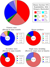 |
Fig. 1. Pie charts of the distribution of supernova types (different colors) from the models assuming the explodability criterion of M16 and the hard-coded merger criteria. The contribution from stars that do not undergo mass transfer is marked with a white hatching. The four lower panels represent the contribution from each progenitor type (primary and secondary stars that were affected by mass transfer, merger products, and single and effectively single stars). The contribution of each channel is given in the center of the respective pie. The legends show the contribution to each supernova type to the whole distribution. We show a comparable plot based on the explodability criteria of PS20 in Fig. 6. |
About one-third of all supernovae are produced by effectively single stars, that is, by stars that never participated in binary mass transfer. The progenitors of about two-thirds of all supernovae are binary interaction products, with merger stars producing ∼30% of all supernovae, and mass donors 23%. Secondary stars that took part in at least one mass-transfer event contribute less (∼16%) because they are the initially less massive component in the binaries and therefore often form WDs.
Primary stars, which are typically mass donors, produce a population of supernovae that differs most strongly from that of single stars. Their majority explode as a Type Ibc supernova, while in particular the long-period binaries with the lowest initial primary masses are not fully stripped and produce Type IIb supernovae (see Fig.D.1). Per definition, the mass donors that reach core collapse during mass transfer produce the interacting supernovae (Types IIn and Ibn).
Secondary stars, merger products, and single stars mostly produce Type IIP/L supernovae. The most massive of them are able to self-strip via winds and also explode, which has a strong effect on the ejecta mass distribution of this class (see below). Notably, this contribution is much smaller when the explodability criterion of PS20 is applied (Sect. 3.2).
3.1.1. Type IIP/L supernovae
Roughly ∼63% of the Type IIP/L supernovae in our synthetic population arise from mass gainers (23%) or mergers (40%) in binary systems (Fig. 2). Overall, these supernovae have ejecta masses of2Mej = 7.5 − 14.4 M⊙, with a pre-explosion envelope mass of MH, env = 2.8 − 11.3 M⊙ (with half of them focused around 6.3 − 7.0 M⊙). These distributions show higher masses and are broader than those expected from single-star evolution (see Appendix B, Mej = 7.6 − 10.7 M⊙ and MH, env = 2.8 − 7.0 M⊙). The absence of more lower-mass envelopes arises from our definition of Type IIb progenitors and because RSGs undergoing case C RLOF typically produce partially stripped envelopes (EJLD24; Fang et al. 2025), but are classified here as Type IIn progenitors and not Type IIP/L.
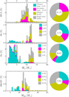 |
Fig. 2. Stacked histograms of the ejecta mass Mej in our fiducial population model grouped by the supernova type (Type IIP/L, IIb, and Type Ibc supernovae) and normalized by the total number of supernovae (in percent). The contribution is split between primary stars (teal), secondary stars (magenta), merger products (dark gold) or single and effectively single stars (gray). The contribution from stars that have not undergone mass transfer is hatched. The pie charts show the relative contribution of different progenitors to each supernova type. The legend also shows the fraction of supernovae within the whole distribution, and their sum is reported inside the pie charts. Separately, we show a histogram for the mass of BHs, with a pie chart showing the relative contribution of different progenitors, and the number is normalized to that of supernovae. Less than one percentile of the distribution of Type IIP/L supernovae and BHs falls outside of the shown ranges, extending up to 43 M⊙. We show a comparable plot based on the explodability criteria of PS20 in Fig. 7. |
While the bulk of secondary-star progenitors of Type IIP/L supernovae have similar ejecta masses to those expected from single-star evolution, they also show a weak high-mass tail from 10.8 to 24.4 M⊙ (which contributes to about 2% of all Type IIP/L supernovae). This high-mass tail is produced in Case A systems in which secondaries accrete significant amounts of mass (as the tides spin them down during mass transfer) and do not rejuvenate.
Merger products have Mej = 7.1 − 17.8 M⊙ and MH, env = 3.1 − 13.8 M⊙. There are a few low-mass outliers (Mej < 7.4 M⊙, making up ≲2% of all Type IIP/L supernovae). These are the products of the mergers in which the preceding phase of mass transfer shed more mass than the mass to which the secondary star contributes. The massive end of the distribution is most remarkable (Mej > 10.8 M⊙, comprising about 14% of all Type IIP/L supernovae). This is produced by Case B mergers, where the addition of the secondary star mass produces an overmassive envelope. Progenitors with these massive hydrogen envelopes are not produced by single stars and are a robust prediction of our binary models, regardless of the adopted merger or explodability criteria.
About 18% of the merger progenitors of Type IIP/L supernovae (corresponding to about 7% of all Type IIP/L supernovae) come from Case A systems with M1, i < 10 M⊙. This is possible because the two stars that initially were not massive enough to have reached core collapse merge to form a more massive star that is able to explode.
3.1.2. Type IIb supernovae
About two-thirds of Type IIb progenitors are produced in mass-transferring binaries (∼68%, Fig. 2). Primaries contribute significantly to this population (27%) and always arise from systems that have undergone late Case B mass transfer (see Fig. D.1). This is in contrast with the discussion about the nature of the progenitor of the prototype Type IIb SN1993J (e.g., Podsiadlowski et al. 1993), which proposed that the progenitor was produced via Case C RLOF. Notably, our models predict that these Case C progenitors would instead give rise to interacting Type II supernovae (see Sects. 2.3). Our models suggest that even at high metallicity, primary stars that underwent Case B RLOF can still retain sufficient hydrogen to appear as a Type IIb supernova.
Secondary stars, merger products, and single stars only become Type IIb supernovae when they are massive enough to self-strip via winds. These models produce very massive Type IIb progenitors, with ejecta masses between 8 and 13 M⊙, which make up ∼73% of them (Fig. 2). We show below that this very massive Type IIb supernova population disappears when the PS20 explodability criterion is used instead of that from M16 (see Fig. 7).
3.1.3. Type Ibc supernovae
Three-quarters of the Type Ibc supernovae are produced in mass-transferring binaries (Fig. 1), and we observe a bimodal distribution in Mej that is very similar to that of the Type IIb progenitors, with 69% of the progenitors located in a broad lower-mass peak (Mej = 1.7 − 6.4 M⊙), and the remaining 31% in a higher-mass peak (Mej = 9.5 − 13.4 M⊙).
The first peak is mostly populated by primary stars that have been fully stripped following RLOF. The secondary stars that contribute to this group are stripped during mass transfer with a BH companion. For 3.5 M⊙ ≤ Mej ≤ 7.0 M⊙, we find a contribution from very massive stars (including those that have not undergone any mass transfer) that end their lives as low-mass He stars at core collapse (see Appendix B). The higher-mass peak centered around ∼12 M⊙ is mostly populated by effectively single stars and merger products. As for the Type IIb progenitors, this high mass peak disappears with the use of the PS20 explodability criterion (see Fig. 7).
3.1.4. 1987A-like supernovae
Only a small number of Case B mergers produce stars with envelopes so massive that they explode while appearing as a blue supergiant. The resulting 87A-like supernovae only account for 0.3% of all core-collapse supernovae, with Mej = 11.5 − 33.1 M⊙. These transients can be quite energetic on average, as Ekin, ej = (1.0 − 5.1)×1051 erg.
3.1.5. Type IIn supernovae
We predict that about 2.4% of all core-collapse supernovae are Type IIn. This number considers all models in which Case C RLOF is triggered after core He depletion. We identified these progenitors in systems in which either the donor star (the primary or secondary star) triggers Case C RLOF with the companion or merger products produced through inverse mass transfer between the secondary star and an evolved primary that already depleted He in the core. This classification was made regardless of how much material was lost during Case C RLOF (ΔMRLOF − C) to form the CSM. We applied thresholds in ΔMRLOF − C above which a model was identified as a Type IIn progenitor. Within reasonable choices for the threshold of 0.01 M⊙ or 0.1 M⊙, the number of identified Type IIn supernovae decreased only slightly (to 2.1% and 1.9%, respectively).
We distinguished the contribution to this population into three groups: objects whose progenitors underwent stable Case C RLOF (26% of all Type IIn supernovae), unstable Case C RLOF (43%), and Case B+C RLOF (31%). Secondaries and merger products also contribute to the population, but by a negligible fraction (Fig. 1), and we neglect their properties in the following statistics. The progenitors undergoing stable Case C RLOF show a higher Mej = 2.5 − 10.0 M⊙ and smaller ΔMRLOF − C ≲ 5.4 M⊙ than those undergoing unstable RLOF (Mej = 1.2 − 4.1 M⊙ and ΔMRLOF − C = 6.6 − 7.0 M⊙, which also includes the mass of the whole H-rich envelope of the donor star before the onset of unstable mass transfer as it also makes up the common envelope). The third group, made up by partially stripped primaries following Case B RLOF, shows lower total masses by the time Case C RLOF begins, and thus exhibits less mass loss (ΔMRLOF − C ≲ 2 M⊙) while maintaining a wide range of ejecta masses (Mej = 1.4 − 8.3 M⊙). All Type IIn supernovae show Ekin, ej = 0.9 − 1.2 × 1051 erg, although this should be taken as an upper limit because most of these progenitors come from low-mass models for which lack reliable estimates of the explosion properties (Sect. 2.2.3).
We show the distribution of the Type IIn supernovae in the Mej–MCSM plane assuming MCSM = ΔMRLOF − C in Fig. 3. The three groups we identified based on their evolutionary history occupy distinct regions in this diagram. When we assume that the CSM is distributed spherically around the progenitor, it follows that the group of unstable Case C systems interacts most strongly (with conversion rates of fM = 0.62 − 0.85; see also the lower panel in Fig. 4), followed by the other two groups that share similar fM < 0.60.
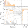 |
Fig. 3. Ejecta masses Mej vs. CSM masses MCSM of our Type IIn supernova progenitors (main panel). The right and upper panels show the MCSM and Mej histograms. The lines in the scatter plot indicate constant fM (Eq. 2), which represents the conversion efficiency of the ejecta kinetic energy into radiation as it impacts the CSM, assuming spherical symmetry. We distinguish the contribution from models undergoing stable Case C (filled orange), unstable Case C (filled blue), and Case C following Case B (empty orange). The inferred properties from a sample of observed Type IIn supernovae from Ransome & Villar (2025) is also shown (gray dots). |
The CSM may have a different geometry depending on whether the mass transfer was stable or unstable. The systems undergoing unstable RLOF might explode while the system is still in-spiralling (EJLD24), and therefore, the CSM might appear as an extended loosely bound and roughly spherical common envelope. The unaccreted material in the models undergoing stable RLOF might be ejected as outflows from the outer Lagrangian points (Lu et al. 2023, EJLD25), which might even remain bound to the inner binary (Pejcha et al. 2016). We assumed that the models undergoing stable RLOF give rise to a flattened CSM, localized within an half-opening angle of 15° from the orbital plane.
Under this assumption, the distribution of Erad is clearly bimodal (Fig. 4, bottom panel; this bimodality is still visible even for half-opening angles up to 30° for stable mass-transferring systems). The high Erad peak is made up of progenitors undergoing unstable Case C RLOF (which we expect to develop a roughly spherical CSM) with fM(90° ) ∼ 0.80 on average, and hence, Erad ≃ fM(90° )Ekin, ej ∼ 8 × 1050 erg. The low Erad peak, made up of systems undergoing stable Case C or Case B+C RLOF, is clearly distinguished from the first as fM(15° ) ∼ 0.1 (Erad ∼ 1050 erg).
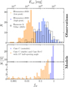 |
Fig. 4. Comparison of the distribution of the integrated bolometric light-curve luminosity Erad of observed Type IIn supernovae (top) and the conversion efficiency fM from our models (bottom). The data from Hiramatsu et al. (2024) distinguish between a high-luminosity group (Erad ∼ 1.8 × 1050 erg, blue) and a low-luminosity group (Erad ∼ 1.4 × 1049 erg, orange), while that of Ransome & Villar (2025) is derived via MOSFIT by fitting and integrating the bolometric light curve for each transient until day 200 after the explosion. The data from Ransome & Villar (2025) were normalized to the total number of transients they analyzed. |
3.1.6. Type Ibn supernovae
Our fiducial model population yields that Type Ibn supernovae make up 2.4% of all core-collapse supernovae (Fig. 1). As in the case of Type IIn supernovae, this number includes all progenitors that underwent mass transfer after core He depletion. When we include a threshold ΔMRLOF − BB ≥ 0.01 M⊙ to identify progenitors of Type Ibn supernovae, the number of these transients only diminishes to 2.2%. We note that the initial parameter space that produces Type Ibn progenitors varies significantly for M1, i = 11.2 M⊙, 12.6 M⊙ and 14 M⊙, which may be a sign that we might be underresolving the progenitor parameter space. We investigated this by interpolating all the models in the grid as a function of initial mass for fixed Pi and qi to identify missing progenitors of Type Ibn supernovae for intermediate M1, i not simulated in the grid. The results agreed with those without the interpolation.
The progenitors of Type Ibn supernovae have ΔMRLOF − BB ≲ 0.77 M⊙ (see Appendix C) and Mej = 0.27 − 1.48 M⊙. While we also obtained Ekin, ej = 1051 erg, we stress that it is likely an overestimate (see Sect. 2.2.3 and EJLD25). Assuming MCSM = ΔMRLOF − BB, we constructed a Mej − MCSM diagram in Fig. 5. Assuming a spherically distributed CSM, we predict that our Type Ibn progenitors would show fM ≲ 0.7.
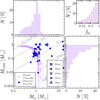 |
Fig. 5. Same diagram as in Fig. 3 for Type Ibn progenitors. We include the inferred properties of the observed Type Ibn previously collected by EJLD25 (see references therein, blue circles) including more recent ones from Wang et al. (2025) (i.e., SN2020nxt, 2020tax, SN2021bbv, SN2023utc, and SN2024aej). In the top right corner, we show a histogram of fM. |
Since these systems all underwent stable Case BB RLOF, we applied the same logic as for stable Case C and Case B+C RLOF, whereby material is likely to be ejected close to the orbital plane and is not spherically distributed. Assuming that the material is found within an half-opening angle of 15° from the orbital plane, we find fM(15° ) ≲ 0.2, which would translate into Erad ≲ 2 × 1050 erg, assuming explosion energies of 1051 erg. The values for fM and Erad are to be taken as upper-limit estimates because we assumed that the mass of the CSM is entirely made up of the mass loss during Case BB (while some part of the material might indeed escape the system and never interact with the supernova), and the explosion energy is likely overestimated (see above).
3.1.7. Black holes
We predict that about seven BHs are formed for every 100 supernovae, with MBH = 7.5 − 19.9 M⊙ (i.e., the pre-collapse mass). This distribution shows a very long high-mass tail that extends to 43 M⊙ and is produced by massive imploding mergers. The lower-mass BHs (≲10 M⊙) are for the most part produced by stripped primary stars.
3.2. The effect of different explodability criteria
We show the results for the fiducial model population (Sect. 3.1) for explodability criteria different from those of M16. For the effect on single-stars, we refer to Appendix B.
When the PS20 method was applied, the relative populations of Type Ibc and Type IIb supernovae decreased. Figure 6 shows that these supernova types lack a contribution from the massive progenitors that were otherwise found in the fiducial population model (Fig. 1). This is a direct consequence of the fact that in effectively single-stars, all progenitors with Mpre − SN ≳ 12 M⊙ implode (Fig. B.1), while most of the binary-stripped progenitors implode for Mpre − SN ≳ 10 M⊙ (Fig. B.2). The population of Type IIb supernovae is exclusively made up of primary stars that were stripped in primaries, while for Type Ibc, the contribution from self-stripped single stars is also negligible. The ejecta masses were restricted to values below ∼8 M⊙.
Type IIP/L supernovae are instead mostly unaffected. This decreases the ratio of Type Ibc to Type IIP/L supernovae (Fig. F.1), but more so for the effectively single-star distribution than for the overall distribution (Fig. 6). Hence, the results over the whole distribution are more sensitive to different choices of fB and to the upper limit on Pi.
The number of interacting supernovae is indirectly affected because they come from a limited mass range in which the progenitors always explode, regardless of the adopted explodability criteria. The increasing number of imploding progenitors of other supernova types increases the relative number of Type IIn and Type Ibn supernovae by ≳1% (Fig. 8). Inevitably, this also increases the ratio of Type Ibn to Type Ibc by ∼0.1, while that of Type IIn to Type IIP/L is unchanged (Fig. F.1).
Because of the more imploding progenitors from both low and high masses, the number of BHs increases to ∼60 per 100 supernovae and shifts the distribution of BH masses to MBH = 5.7 − 16.3 M⊙ (compared to 7.5 − 19.9 M⊙ when using M16). Not only are BHs more numerous, they also show a double-peaked distribution, with one peak around 4.4 − 8.6 M⊙ (about 24% of the formed BHs) and the other peak around 11.6 − 18.1 M⊙ (76%). Additionally, the high-mass tail in their distribution now extends to even higher masses, up to 55 M⊙.
With the explodability criterion from E16, only the fractions of Type IIP/L and Type Ibc supernovae are significantly affected (Fig. 8, F.1) when compared to the fiducial model, but to a lesser extent than when the criterion of PS20 is employed. About 16 BHs are produced per 100 supernovae, with typical BH masses MBH = 7.0 − 15.3 M⊙.
4. Comparison to observations
Several works have collected supernova observations and provided statistics on their distributions that can be compared to stellar models. Volume-limited samples are the preferred comparison tools because they provide estimates that compensate for the magnitude bias. We compared our models with the samples from Eldridge et al. (2013, an updated sample from Smartt et al. 2009), the subsample from high-mass galaxies from the Lick Observatory Supernova Search survey (LOSS) from Graur et al. (2017, initially reported by Li et al. 2011 and reanalyzed in Shivvers et al. 2017a; the data in high-mass galaxies should correspond to high-metallicity environments, Tremonti et al. 2004; Bevacqua et al. 2024, which better compares to our models), Ma et al. (2025b), and the sample from ASAS-SN (Pessi et al. 2025).
4.1. Type IIP/L, IIb, and Ibc supernovae
The fraction of Type IIP/L supernovae in our fiducial population model is within the ranges inferred by the observational samples (see Fig. 8). The closest choice of model parameters that best agrees with the average values reported in these studies are those with the fewest implosions (i.e., the criterion from M16) and the fewest mergers (i.e., the hard-coded merger criteria). Models with any combination of merger and explosion criteria are still found within the error bars of the observations, however, with the exception of the model that combined the most mergers and the most implosions. Das et al. (2025) showed that the low-luminosity Type IIP supernovae (referred to as LLIIP) cannot be associated with single stars with a mass between 8 and 12 M⊙. In our models, the population of Type IIP/L supernovae originating from this mass range is reduced through binary-induced stripping, accretion, and mergers, which alleviates this difference.
The observed fraction of Type Ibc supernovae is less constrained, with some sources estimating ∼25 − 30% (Eldridge et al. 2013, Graur et al. 2017), which agreed well with our models, preferentially with those with fewer mergers and implosions (although the observational error bars are still compatible with all models, except for those with the most mergers or most implosions). No similar conclusion can be drawn when we compare our models to the estimates from Ma et al. (2025b) and Pessi et al. (2025), where the observations yielded a small number of Type Ibc supernovae (∼20%), which in this case agrees better with models showing more mergers or more implosions. There is observational evidence for a few Type Ibc supernova progenitors having been massive and likely not originating from binary stripping (e.g., Taddia et al. 2019; Karamehmetoglu et al. 2023, but see Dessart et al. 2020 for possible degeneracies), which is compatible with our fiducial population model (see Sect. 3.1 and Fig. 2), but not with models in which all massive progenitors always implode (see Sect. 3.2 and Fig.7).
For the observed ratio of Type Ibc to Type IIP/L (Fig. F.1), Eldridge et al. (2013) and Graur et al. (2017) estimated a value of ∼0.45 − 0.48, which is compatible with our models when fewer mergers and implosions are produced. The results of Ma et al. (2025b) and Pessi et al. (2025) yielded a ratio of 0.30 − 0.35, which instead agrees with models with more mergers or more implosions (Fig. F.1).
Type IIb supernovae make up about 10% of the observed events in different volume-limited samples (Eldridge et al. 2013; Graur et al. 2017; Ma et al. 2025b; Pessi et al. 2025), which is much greater than our predicted numbers regardless of the chosen set of parameters (Fig. 8). This might be connected to the wind mass-loss recipes adopted in the stellar evolutionary models, which strip low-mass H-rich envelopes too efficiently (see Appendix A.1.1), or to inconsistencies in the classification of Type IIb supernovae in models and observations. Moreover, the bulk of Type IIb supernovae is expected to come from stars that underwent binary interaction (Smith et al. 2011), while our fiducial population models suggest the opposite. Nonetheless, some observations of Type IIb supernovae have suggested a high-mass progenitor (e.g., Rubin & Gal-Yam 2016).
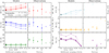 |
Fig. 8. Comparison between the predictions on the fractions of supernovae of different types (different blocks) produced by the models (left subpanel, with our supernova nomenclature on the left y-axis) and the observed fractions (right subpanel, with the observed subtypes that we clumped in each group on the right y-axis). The numbers are reported as a fraction of all core-collapse supernovae. For the models, a line plot show the variation of the fraction of supernovae subtypes as a function of different merger criteria added on top of the hard-coded criteria (‘None’ on the x-axis), sorted from left to right by those that produce less to more mergers that reach core collapse (see text). Different dashes shows the same while assuming different explodability criteria sorted by increasing number of implosions, that all stars successfully explode (All), Müller et al. (2016, M16), Ertl et al. (2016, E16), and Patton & Sukhbold (2020, PS20). The star corresponds to the fiducial model. For the observation, we show the estimates from volume-limited samples from Eldridge et al. 2013 (E13), the LOSS survey (specifically, the subsample from high-mass galaxies, which serves as a proxy of high-metallicity environments; Graur et al. 2017), and the samples from Ma et al. 2025b (M25) and ASAS-SN (Pessi et al. 2025) with filled markers. We also include for reference the magnitude-limited samples from PTF (Schulze et al. 2021) and ZTF (Hinds et al. 2025), shown with empty markers. |
Our estimates for the fraction of 87A-like supernovae are compatible with those from Eldridge et al. (2013), and the nondetections from high-mass galaxies from Graur et al. (2017). Ma et al. (2025b) instead found a fraction of 87A-like supernovae closer to 2%, which is distinctly higher than even our more optimistic estimate when we assumed more mergers. While this fraction might be larger when secondary and primary stars are included (which we excluded because of MLT++; see Sects. 2.3 and Appendix A.1.2), this would additionally decrease the number of Type IIb supernovae, which already differ with observations.
4.2. Type IIn supernovae
Eldridge et al. (2013), Graur et al. (2017) and, Pessi et al. (2025) indicated a relative number of Type IIn of about 2 − 4% of all core-collapse supernovae, which is compatible with our estimates. Ma et al. 2025b instead recently reported a number of Type IIn supernovae closer to 5.6% of all core-collapse supernovae, which is higher by about a factor of two than our predictions.
A large-scale attempt to fit numerous Type IIn supernova light curves was made by Ransome & Villar (2025), who analyzed 147 transients using the code MOSFIT (Chatzopoulos et al. 2012; Guillochon et al. 2018). Their analysis revealed that most of the observed Type IIn supernovae had  and
and  . These values differ from those derived within the framework of our models (see Fig. 3), although some events singularly overlap with our models. These massive events might be the result of a non-volume-limited sampling, which may be biased toward more luminous and extreme events likely from more uncommon evolutionary channels such as pulsational pair-instability (PPI, Woosley 2017) or LBV-like eruptions (e.g., for the progenitor of SN2010jl, Niu et al. 2024), which we did not consider in our models.
We caution that the assumption of spherical geometry for modeling the CSM interaction in MOSFIT might affect the inferred fitting parameters for interacting supernovae where the CSM is asymmetrically distributed. Several observations of Type IIn supernovae such as SN2012ab (Bilinski et al. 2018), SN2013L (Andrews et al. 2017), and SN2020ywx (Baer-Way et al. 2025) highlighted an asymmetric CSM at the time of explosion. This has also been observed for the Type II SN2023ixf (Vasylyev et al. 2025). Surveys of Type IIn supernovae via spectropolarimetry (Bilinski et al. 2024) and UV and optical studies of their light curves (Soumagnac et al. 2020) suggested that a strong asymmetry in the CSM was found for ∼35 − 66% of all Type IIn supernovae. This indicates that perhaps all Type IIn supernovae have an asymmetric CSM when considering the random viewing angle distribution of the observer with respect to the CSM (Bilinski et al. 2024). Other events, such as SN2014C, can be explained in the context of interaction with a toroidal CSM (Bietenholz et al. 2021) which can be produced in a 1000-year-long enhanced mass loss through a binary companion (Milisavljevic et al. 2015; Orlando et al. 2024) without necessarily being driven by common-envelope evolution because stable mass transfer can still provide a bound, massive, and aspherical CSM.
A more comprehensive sample of 475 Type IIn supernovae has been reported by Hiramatsu et al. (2024). The authors noted that the transients showed a bimodal distribution of their integrated light-curve luminosities, with one group showing Erad ∼ 1.4 × 1049 erg and a second group with Erad ∼ 1.8 × 1050 erg. This bimodality is qualitatively similar to that we found in the models (see Fig. 4), although our peaks are found at higher Erad (assuming Ekin, ej ∼ 1051 erg in our models). This difference is expected because we assumed that all of ΔMRLOF − C interacts with the supernova. As some of it might be unbound from the binary and never interact with the supernova, the effective value of fM might be substantially lower and hence offer a way to reconcile our Erad with the observation. We also note that the relative number of systems undergoing unstable versus stable Case C plus Case B+C RLOF (43% to 57%) is similar to that of low- versus high-luminosity groups in Hiramatsu et al. (2024, 51% to 49%), even though the observations do not provide a volume-limited sample and hence might overrepresent high-luminosity transients.
Finally, our models do not predict the occurrence of outburst prior to the explosion, as observed in many Type IIn supernovae (Ofek et al. 2014; Strotjohann et al. 2021; Reguitti et al. 2024). We refer to Appendix A.3 for a discussion.
4.3. Type Ibn supernovae
Hosseinzadeh et al. (2017) collected Type Ibn supernovae to construct a template light curve of these objects, with which typical radiated energies of these transients of Erad = (1.6 − 3.8)×1049 erg can be derived. This value is lower by about a factor of three than what we predicted from the models when we assumed that the CSM is focused closer to the orbital plane. Significantly lower explosion energies (EJLD25) and lower CSM masses in the models can push Erad closer to the observed values, however.
For some of the observed supernovae, a light-curve fit has produced estimates for the CSM and ejecta masses. Much like the case of Type IIn supernovae, some outliers have exceptionally high energies and/or high inferred ejecta masses, which might be produced through PPI (Woosley 2017). In addition, the bulk of these observations seems to coincide with the parameter space predicted by our models (see EJLD25). Interestingly, the region occupied by most observations in Fig. 5 coincides with the more populated region theoretically (within the lines fM = 0.1 and fM = 0.5). We nonetheless remain cautious of the inferred masses from these events because some of them show signs of asymmetry in the CSM (e.g., SN2023fyq, Dong et al. 2024). The asymmetry would likely affect the estimates of MCSM and Mej from a light-curve fit because spherical symmetry was assumed in these models.
Until recently, no estimates of the fraction of Type Ibn supernovae with respect to the population of core-collapse supernovae were available. Works from PTF (Schulze et al. 2021) and ZTF (Perley et al. 2020; Hinds et al. 2025) reported that Type Ibn supernovae seem to contribute about 1 − 3% of all supernovae within a magnitude-limited sample. The first volume-limited estimates of Type Ibn supernovae came from Ma et al. (2025b) and Pessi et al. (2025). Ma et al. (2025b) suggested that Type Ibn supernovae contribute to about 2% to all core-collapse supernovae (Fig. 8), with a ratio of Type Ibn to Type Ibc of about 0.1. While the uncertainties on this number are quite large, it is compatible with the results of our fiducial model. The number of Type Ibn supernovae and their ratio to Type Ibc are both incompatible with the population models assuming the energy’ criterion for mergers or the PS20 criterion for explodability. Moreover, the other merger and explodability criteria combinations produce fractions of Type Ibn supernovae that are compatible with the observed value.
Pessi et al. (2025) instead observed only 0.5%±0.4% of all core-collapse supernovae as Type Ibn. This small fraction is only found in models with the energy merger criterion, which directly contrasts with the conclusions inferred from comparing our models to the results of Ma et al. (2025b).
5. Conclusions
We have found that about two-thirds of all Type IIP/L supernova progenitors are expected to have experienced mass accretion or merging. Therefore, binary evolution can lead to much higher envelope masses and ejecta masses than single-star evolution (Fig. 1). Our models also predict a small population of SN1987A-like transients from massive merger products based on a high final envelope-to-core mass ratio.
Binary evolution naturally enhances the number of stripped-envelope supernovae (Type Ibc and Type IIb), and leads to a number ratio of Type Ibc to Type IIP/L that roughly agrees with the observed ratio. In particuar, it enables a copious number of low-mass Type Ibc and Type IIb supernovae via binary-stripped primaries and secondaries (Fig. 2).
Our models also showed a strong dependence of the progenitor and ejecta mass distribution of stripped-envelope supernovae on the employed explodability criteria. We found that the M16 criteria lead to a supernova population that is very similar to the population found when assuming that all massive stars explode (because it only forms 7 BHs per 100 supernovae). This leads to most Type IIb and one-third of Type Ibc supernovae showing ejecta masses of ≳12 M⊙ (Fig. 2). With the explodability criteria of PS20, on the other hand, we obtained 60 BH per 100 SNe, and the massive progenitors of Type IIb and Type Ibc all implode (Fig. 7).
Our comprehensive and dense grid of binary evolution models also allowed us a first assessment of the expected population of interacting supernovae in the frame of our assumption that a core-collapse supernova arising during mass transfer gives rise to this phenomenon (EJLD24, EJLD25). Our models predict that Type IIn supernovae make up 2.4% of all core-collapse supernovae, which is consistent with volume-limited supernova samples (Eldridge et al. 2013; Graur et al. 2017). Similarly, Type Ibn supernovae make up 2.4% of all core-collapse supernovae, which is compatible with the value derived in the volume-limited sample by Ma et al. (2025b). Furthermore, our models showed a bimodal distribution of radiated energies of Type IIn events, which qualitatively agrees with observations (Hiramatsu et al. 2024), when stable mass transfer is assumed to produce disk-like CSM structures, while unstable mass transfer yields more spherical outflows.
The high-cadence observations of transients from the concurrent operations of LSST and ZTF, along with a continued analysis of archival data from current programs, will provide invaluable insights into the populations of observed supernovae. In particular, focused efforts on identifying and characterizing interacting supernovae will provide critical constraints on the final phases of stellar evolution and the nature of mass loss near core-collapse.
Acknowledgments
This project made use of the Julia language (Bezanson et al. 2017). All plots were made with the Makie.jl package (Danisch & Krumbiegel 2021). The authors thank the anonymous reviewer for their valuable and constructive feedback, which has significantly contributed to the enhancement of this manuscript. The authors additionally express their gratitude to Luc Dessart for inspiring ideas and comments, as well as to Adam Burrows and Qiliang Fang for constructive comments. AE thanks Fabian Schneider for sharing data from his models and for helpful discussions. AE is also grateful for many insightful discussions with Eva Laplace, Philip Podsiadlowski, Vincent Bronner, Ruggero Valli, Alexander Heger, Ylva Götberg, Reinhold Willcox, and Bethany Ludwig.
References
- Aguilera-Dena, D. R., Langer, N., Moriya, T. J., & Schootemeijer, A. 2018, ApJ, 858, 115 [NASA ADS] [CrossRef] [Google Scholar]
- Aguilera-Dena, D. R., Langer, N., Antoniadis, J., et al. 2022, A&A, 661, A60 [NASA ADS] [CrossRef] [EDP Sciences] [Google Scholar]
- Aguilera-Dena, D. R., Müller, B., Antoniadis, J., et al. 2023, A&A, 671, A134 [NASA ADS] [CrossRef] [EDP Sciences] [Google Scholar]
- Almeida, L. A., Sana, H., Taylor, W., et al. 2017, A&A, 598, A84 [NASA ADS] [CrossRef] [EDP Sciences] [Google Scholar]
- Andrews, J. E., Smith, N., McCully, C., et al. 2017, MNRAS, 471, 4047 [Google Scholar]
- Antoniadis, K., Bonanos, A. Z., de Wit, S., et al. 2024, A&A, 686, A88 [NASA ADS] [CrossRef] [EDP Sciences] [Google Scholar]
- Arroyo-Torres, B., Wittkowski, M., Chiavassa, A., et al. 2015, A&A, 575, A50 [NASA ADS] [CrossRef] [EDP Sciences] [Google Scholar]
- Backs, F., Brands, S. A., de Koter, A., et al. 2024, A&A, 692, A88 [NASA ADS] [CrossRef] [EDP Sciences] [Google Scholar]
- Baer-Way, R., Chandra, P., Modjaz, M., et al. 2025, ApJ, 983, 101 [Google Scholar]
- Bellm, E. C., Kulkarni, S. R., Graham, M. J., et al. 2019, PASP, 131, 018002 [Google Scholar]
- Bersten, M. C., Benvenuto, O. G., Folatelli, G., et al. 2014, AJ, 148, 68 [NASA ADS] [CrossRef] [Google Scholar]
- Bevacqua, D., Saracco, P., Boecker, A., et al. 2024, A&A, 690, A150 [NASA ADS] [CrossRef] [EDP Sciences] [Google Scholar]
- Bezanson, J., Edelman, A., Karpinski, S., & Shah, V. B. 2017, SIAM Rev., 59, 65 [Google Scholar]
- Bietenholz, M. F., Bartel, N., Kamble, A., et al. 2021, MNRAS, 502, 1694 [Google Scholar]
- Bilinski, C., Smith, N., Williams, G. G., et al. 2018, MNRAS, 475, 1104 [Google Scholar]
- Bilinski, C., Smith, N., Williams, G. G., et al. 2024, MNRAS, 529, 1104 [Google Scholar]
- Brandt, N., & Podsiadlowski, P. 1995, MNRAS, 274, 461 [NASA ADS] [CrossRef] [Google Scholar]
- Braun, H., & Langer, N. 1995, A&A, 297, 483 [NASA ADS] [Google Scholar]
- Bronner, V. A., Schneider, F. R. N., Podsiadlowski, P., & Röpke, F. K. 2024, A&A, 683, A65 [NASA ADS] [CrossRef] [EDP Sciences] [Google Scholar]
- Bronner, V. A., Laplace, E., Schneider, F. R. N., & Podsiadlowski, P. 2025, A&A, 703, A61 [NASA ADS] [CrossRef] [EDP Sciences] [Google Scholar]
- Brott, I., de Mink, S. E., Cantiello, M., et al. 2011, A&A, 530, A115 [NASA ADS] [CrossRef] [EDP Sciences] [Google Scholar]
- Brown, G. E., Heger, A., Langer, N., et al. 2001, New Astron., 6, 457 [NASA ADS] [CrossRef] [Google Scholar]
- Burrows, A., & Vartanyan, D. 2021, Nature, 589, 29 [CrossRef] [PubMed] [Google Scholar]
- Burrows, A., Wang, T., & Vartanyan, D. 2025, ApJ, 987, 164 [Google Scholar]
- Chan, C., Müller, B., Heger, A., Pakmor, R., & Springel, V. 2018, ApJ, 852, L19 [NASA ADS] [CrossRef] [Google Scholar]
- Chatzopoulos, E., Wheeler, J. C., & Vinko, J. 2012, ApJ, 746, 121 [Google Scholar]
- Chevalier, R. A. 1989, ApJ, 346, 847 [Google Scholar]
- Claeys, J. S. W., de Mink, S. E., Pols, O. R., Eldridge, J. J., & Baes, M. 2011, A&A, 528, A131 [NASA ADS] [CrossRef] [EDP Sciences] [Google Scholar]
- Colgate, S. A. 1971, ApJ, 163, 221 [Google Scholar]
- Danisch, S., & Krumbiegel, J. 2021, J. Open Source Software, 6, 3349 [NASA ADS] [CrossRef] [Google Scholar]
- Darwin, G. H. 1879, Proc. Royal Soc. London Ser., I(29), 168 [Google Scholar]
- Das, K. K., Kasliwal, M. M., Fremling, C., et al. 2025, PASP, 137, 044203 [Google Scholar]
- De Donder, E., Vanbeveren, D., & van Bever, J. 1997, A&A, 318, 812 [NASA ADS] [Google Scholar]
- Dessart, L., Hillier, D. J., Livne, E., et al. 2011, MNRAS, 414, 2985 [NASA ADS] [CrossRef] [Google Scholar]
- Dessart, L., Hillier, D. J., Li, C., & Woosley, S. 2012, MNRAS, 424, 2139 [NASA ADS] [CrossRef] [Google Scholar]
- Dessart, L., Hillier, D. J., Waldman, R., & Livne, E. 2013, MNRAS, 433, 1745 [NASA ADS] [CrossRef] [Google Scholar]
- Dessart, L., Hillier, D. J., Woosley, S., et al. 2015, MNRAS, 453, 2189 [NASA ADS] [CrossRef] [Google Scholar]
- Dessart, L., Hillier, D. J., Woosley, S., et al. 2016, MNRAS, 458, 1618 [NASA ADS] [CrossRef] [Google Scholar]
- Dessart, L., Yoon, S.-C., Aguilera-Dena, D. R., & Langer, N. 2020, A&A, 642, A106 [NASA ADS] [CrossRef] [EDP Sciences] [Google Scholar]
- Dessart, L., Gutiérrez, C. P., Ercolino, A., Jin, H., & Langer, N. 2024, A&A, 685, A169 [NASA ADS] [CrossRef] [EDP Sciences] [Google Scholar]
- Dong, Y., Tsuna, D., Valenti, S., et al. 2024, ApJ, 977, 254 [Google Scholar]
- Drout, M. R., Soderberg, A. M., Gal-Yam, A., et al. 2011, ApJ, 741, 97 [NASA ADS] [CrossRef] [Google Scholar]
- Dufton, P. L., Langer, N., Dunstall, P. R., et al. 2013, A&A, 550, A109 [NASA ADS] [CrossRef] [EDP Sciences] [Google Scholar]
- Eldridge, J. J., Izzard, R. G., & Tout, C. A. 2008, MNRAS, 384, 1109 [Google Scholar]
- Eldridge, J. J., Langer, N., & Tout, C. A. 2011, MNRAS, 414, 3501 [NASA ADS] [CrossRef] [Google Scholar]
- Eldridge, J. J., Fraser, M., Smartt, S. J., Maund, J. R., & Crockett, R. M. 2013, MNRAS, 436, 774 [NASA ADS] [CrossRef] [Google Scholar]
- Eldridge, J. J., Stanway, E. R., Xiao, L., et al. 2017, PASA, 34, e058 [Google Scholar]
- Ercolino, A., Jin, H., Langer, N., & Dessart, L. 2024, A&A, 685, A58 [NASA ADS] [CrossRef] [EDP Sciences] [Google Scholar]
- Ercolino, A., Jin, H., Langer, N., & Dessart, L. 2025, A&A, 696, A103 [NASA ADS] [CrossRef] [EDP Sciences] [Google Scholar]
- Ertl, T., Janka, H. T., Woosley, S. E., Sukhbold, T., & Ugliano, M. 2016, ApJ, 818, 124 [NASA ADS] [CrossRef] [Google Scholar]
- Ertl, T., Woosley, S. E., Sukhbold, T., & Janka, H. T. 2020, ApJ, 890, 51 [CrossRef] [Google Scholar]
- Fang, Q., Moriya, T. J., Maeda, K., Dorozsmai, A., & Silva-Farfán, J. 2025, ApJ, 990, 60 [Google Scholar]
- Fremling, C., Sollerman, J., Taddia, F., et al. 2014, A&A, 565, A114 [NASA ADS] [CrossRef] [EDP Sciences] [Google Scholar]
- Fryer, C. L. 1999, ApJ, 522, 413 [NASA ADS] [CrossRef] [Google Scholar]
- Fuller, J. 2017, MNRAS, 470, 1642 [NASA ADS] [CrossRef] [Google Scholar]
- Gagnier, D., & Pejcha, O. 2023, A&A, 674, A121 [NASA ADS] [CrossRef] [EDP Sciences] [Google Scholar]
- Gagnier, D., & Pejcha, O. 2025, A&A, 697, A68 [NASA ADS] [CrossRef] [EDP Sciences] [Google Scholar]
- Gal-Yam, A. 2017, in Handbook of Supernovae, eds. A. W. Alsabti, & P. Murdin, 195 [Google Scholar]
- Gal-Yam, A., Bruch, R., Schulze, S., et al. 2022, Nature, 601, 201 [NASA ADS] [CrossRef] [Google Scholar]
- Georgy, C., Meynet, G., Walder, R., Folini, D., & Maeder, A. 2009, A&A, 502, 611 [NASA ADS] [CrossRef] [EDP Sciences] [Google Scholar]
- Gilkis, A., & Arcavi, I. 2022, MNRAS, 511, 691 [NASA ADS] [CrossRef] [Google Scholar]
- Gilkis, A., Vink, J. S., Eldridge, J. J., & Tout, C. A. 2019, MNRAS, 486, 4451 [CrossRef] [Google Scholar]
- Gilkis, A., Laplace, E., Arcavi, I., Shenar, T., & Schneider, F. R. N. 2025, MNRAS, 540, 3094 [Google Scholar]
- Goldberg, J. A., Bildsten, L., & Paxton, B. 2019, ApJ, 879, 3 [Google Scholar]
- Götberg, Y., Drout, M. R., Ji, A. P., et al. 2023, ApJ, 959, 125 [CrossRef] [Google Scholar]
- Graur, O., Bianco, F. B., Modjaz, M., et al. 2017, ApJ, 837, 121 [CrossRef] [Google Scholar]
- Groh, J. H., Meynet, G., Georgy, C., & Ekström, S. 2013, A&A, 558, A131 [NASA ADS] [CrossRef] [EDP Sciences] [Google Scholar]
- Guillochon, J., Nicholl, M., Villar, V. A., et al. 2018, ApJS, 236, 6 [NASA ADS] [CrossRef] [Google Scholar]
- Hachinger, S., Mazzali, P. A., Taubenberger, S., et al. 2012, MNRAS, 422, 70 [NASA ADS] [CrossRef] [Google Scholar]
- Hainich, R., Pasemann, D., Todt, H., et al. 2015, A&A, 581, A21 [NASA ADS] [CrossRef] [EDP Sciences] [Google Scholar]
- Hatfull, R. W. M., & Ivanova, N. 2025, ApJ, 982, 83 [Google Scholar]
- Heger, A., Jeannin, L., Langer, N., & Baraffe, I. 1997, A&A, 327, 224 [NASA ADS] [Google Scholar]
- Heger, A., Langer, N., & Woosley, S. E. 2000, ApJ, 528, 368 [NASA ADS] [CrossRef] [Google Scholar]
- Hellings, P. 1983, Ap&SS, 96, 37 [NASA ADS] [CrossRef] [Google Scholar]
- Hinds, K.-R., Perley, D. A., Sollerman, J., et al. 2025, MNRAS, 541, 135 [Google Scholar]
- Hirai, R., & Mandel, I. 2022, ApJ, 937, L42 [NASA ADS] [CrossRef] [Google Scholar]
- Hiramatsu, D., Berger, E., Gomez, S., et al. 2024, ArXiv e-prints [arXiv:2411.07287] [Google Scholar]
- Hosseinzadeh, G., Arcavi, I., Valenti, S., et al. 2017, ApJ, 836, 158 [Google Scholar]
- Humphreys, R. M., & Davidson, K. 1979, ApJ, 232, 409 [Google Scholar]
- Ivanova, N., Justham, S., Avendano Nandez, J. L., & Lombardi, J. C. 2013, Science, 339, 433 [NASA ADS] [CrossRef] [Google Scholar]
- Ivanova, N., Justham, S., & Ricker, P. 2020, Common Envelope Evolution [Google Scholar]
- Janka, H.-T. 2025, Ann. Rev. Nucl. Part. Sci., 75, 425 [Google Scholar]
- Jin, H., Yoon, S.-C., & Blinnikov, S. 2023, ApJ, 950, 44 [Google Scholar]
- Jin, H., Langer, N., Lennon, D. J., & Proffitt, C. R. 2024, A&A, 690, A135 [NASA ADS] [CrossRef] [EDP Sciences] [Google Scholar]
- Jin, H., Langer, N., Ercolino, A., & de Mink, S. E. 2025, ArXiv e-prints [arXiv:2510.19965] [Google Scholar]
- Justham, S., Podsiadlowski, P., & Vink, J. S. 2014, ApJ, 796, 121 [NASA ADS] [CrossRef] [Google Scholar]
- Karamehmetoglu, E., Sollerman, J., Taddia, F., et al. 2023, A&A, 678, A87 [NASA ADS] [CrossRef] [EDP Sciences] [Google Scholar]
- Kee, N. D., Sundqvist, J. O., Decin, L., de Koter, A., & Sana, H. 2021, A&A, 646, A180 [NASA ADS] [CrossRef] [EDP Sciences] [Google Scholar]
- Kinugawa, T., Inayoshi, K., Hotokezaka, K., Nakauchi, D., & Nakamura, T. 2014, MNRAS, 442, 2963 [NASA ADS] [CrossRef] [Google Scholar]
- Kinugawa, T., Miyamoto, A., Kanda, N., & Nakamura, T. 2016, MNRAS, 456, 1093 [CrossRef] [Google Scholar]
- Kinugawa, T., Horiuchi, S., Takiwaki, T., & Kotake, K. 2024, MNRAS, 532, 3926 [NASA ADS] [CrossRef] [Google Scholar]
- Klencki, J., Podsiadlowski, P., Langer, N., et al. 2026, A&A, in press, https://doi.org/10.1051/0004-6361/202555500 [Google Scholar]
- Ko, T., Kinugawa, T., Tsuna, D., Hirai, R., & Takei, Y. 2025, MNRAS, 541, 3747 [Google Scholar]
- Kolb, U., & Ritter, H. 1990, A&A, 236, 385 [NASA ADS] [Google Scholar]
- Kroupa, P., Aarseth, S., & Hurley, J. 2001, MNRAS, 321, 699 [NASA ADS] [CrossRef] [Google Scholar]
- Kuncarayakti, H., Maeda, K., Bersten, M. C., et al. 2015, A&A, 579, A95 [CrossRef] [EDP Sciences] [Google Scholar]
- Langer, N. 2012, ARA&A, 50, 107 [CrossRef] [Google Scholar]
- Laplace, E., Justham, S., Renzo, M., et al. 2021, A&A, 656, A58 [NASA ADS] [CrossRef] [EDP Sciences] [Google Scholar]
- Laplace, E., Bronner, V. A., Schneider, F. R. N., & Podsiadlowski, P. 2025, ArXiv e-prints [arXiv:2508.11088] [Google Scholar]
- Lau, M. Y. M., Hirai, R., González-Bolívar, M., et al. 2022, MNRAS, 512, 5462 [NASA ADS] [CrossRef] [Google Scholar]
- Lau, M. Y. M., Hirai, R., Price, D. J., Mandel, I., & Bate, M. R. 2025, A&A, 699, A274 [NASA ADS] [CrossRef] [EDP Sciences] [Google Scholar]
- Law, N. M., Kulkarni, S. R., Dekany, R. G., et al. 2009, PASP, 121, 1395 [NASA ADS] [CrossRef] [Google Scholar]
- Li, W., Leaman, J., Chornock, R., et al. 2011, MNRAS, 412, 1441 [NASA ADS] [CrossRef] [Google Scholar]
- Lu, W., Fuller, J., Quataert, E., & Bonnerot, C. 2023, MNRAS, 519, 1409 [Google Scholar]
- Ma, J. Z., Justham, S., Pakmor, R., et al. 2025a, ArXiv e-prints [arXiv:2510.14875] [Google Scholar]
- Ma, X., Wang, X., Mo, J., et al. 2025b, A&A, 698, A305 [NASA ADS] [CrossRef] [EDP Sciences] [Google Scholar]
- Mac Low, M.-M., & Klessen, R. S. 2004, Rev. Modern Phys., 76, 125 [NASA ADS] [CrossRef] [Google Scholar]
- Mac Low, M.-M., Balsara, D. S., Kim, J., & de Avillez, M. A. 2005, ApJ, 626, 864 [NASA ADS] [CrossRef] [Google Scholar]
- Maltsev, K., Schneider, F. R. N., Mandel, I., et al. 2025, A&A, 700, A20 [NASA ADS] [CrossRef] [EDP Sciences] [Google Scholar]
- Marchant, P. 2017, Ph.D. Thesis, Rheinische Friedrich Wilhelms University of Bonn, Germany [Google Scholar]
- Marchant, P., Pappas, K. M. W., Gallegos-Garcia, M., et al. 2021, A&A, 650, A107 [NASA ADS] [CrossRef] [EDP Sciences] [Google Scholar]
- Martinez, L., Bersten, M. C., Anderson, J. P., et al. 2022, A&A, 660, A41 [NASA ADS] [CrossRef] [EDP Sciences] [Google Scholar]
- Matsuoka, T., & Sawada, R. 2024, ApJ, 963, 105 [NASA ADS] [CrossRef] [Google Scholar]
- McKee, C. F., & Ostriker, J. P. 1977, ApJ, 218, 148 [NASA ADS] [CrossRef] [Google Scholar]
- Menon, A., & Heger, A. 2017, MNRAS, 469, 4649 [NASA ADS] [Google Scholar]
- Menon, A., Langer, N., de Mink, S. E., et al. 2021, MNRAS, 507, 5013 [NASA ADS] [CrossRef] [Google Scholar]
- Menon, A., Ercolino, A., Urbaneja, M. A., et al. 2024, ApJ, 963, L42 [NASA ADS] [CrossRef] [Google Scholar]
- Meynet, G., & Maeder, A. 2005, A&A, 429, 581 [CrossRef] [EDP Sciences] [Google Scholar]
- Milisavljevic, D., Margutti, R., Kamble, A., et al. 2015, ApJ, 815, 120 [NASA ADS] [CrossRef] [Google Scholar]
- Moe, M., & Di Stefano, R. 2017, ApJS, 230, 15 [Google Scholar]
- Mokiem, M. R., de Koter, A., Vink, J. S., et al. 2007, A&A, 473, 603 [NASA ADS] [CrossRef] [EDP Sciences] [Google Scholar]
- Moriya, T. J., Blinnikov, S. I., Tominaga, N., et al. 2013, MNRAS, 428, 1020 [NASA ADS] [CrossRef] [Google Scholar]
- Müller, B., Heger, A., Liptai, D., & Cameron, J. B. 2016, MNRAS, 460, 742 [Google Scholar]
- Nieuwenhuijzen, H., & de Jager, C. 1990, A&A, 231, 134 [NASA ADS] [Google Scholar]
- Niu, Z., Sun, N.-C., & Liu, J. 2024, ApJ, 966, L20 [Google Scholar]
- Nomoto, K., Tominaga, N., Umeda, H., Kobayashi, C., & Maeda, K. 2006, Nucl. Phys. A, 777, 424 [CrossRef] [Google Scholar]
- Nugis, T., & Lamers, H. J. G. L. M. 2000, A&A, 360, 227 [NASA ADS] [Google Scholar]
- O’Connor, E., & Ott, C. D. 2011, ApJ, 730, 70 [Google Scholar]
- Ofek, E. O., Sullivan, M., Shaviv, N. J., et al. 2014, ApJ, 789, 104 [NASA ADS] [CrossRef] [Google Scholar]
- Offner, S. S. R., Moe, M., Kratter, K. M., et al. 2023, ASP Conf. Ser., 534, 275 [NASA ADS] [Google Scholar]
- Orlando, S., Greco, E., Hirai, R., et al. 2024, ApJ, 977, 118 [Google Scholar]
- Ouchi, R., & Maeda, K. 2017, ApJ, 840, 90 [NASA ADS] [CrossRef] [Google Scholar]
- Paczynski, B. 1976, in Structure and Evolution of Close Binary Systems, eds. P. Eggleton, S. Mitton, & J. Whelan, 73, 75 [NASA ADS] [CrossRef] [Google Scholar]
- Pastorello, A., Mattila, S., Zampieri, L., et al. 2008, MNRAS, 389, 113 [Google Scholar]
- Pastorello, A., Mason, E., Taubenberger, S., et al. 2019, A&A, 630, A75 [NASA ADS] [CrossRef] [EDP Sciences] [Google Scholar]
- Patton, R. A., & Sukhbold, T. 2020, MNRAS, 499, 2803 [NASA ADS] [CrossRef] [Google Scholar]
- Pauli, D. 2020, Master’s Thesis, Rheinische Friedrich Wilhelms University ofBonn, Germany [Google Scholar]
- Pauli, D., Langer, N., Aguilera-Dena, D. R., Wang, C., & Marchant, P. 2022, A&A, 667, A58 [NASA ADS] [CrossRef] [EDP Sciences] [Google Scholar]
- Pavlovskii, K., & Ivanova, N. 2015, MNRAS, 449, 4415 [Google Scholar]
- Paxton, B., Bildsten, L., Dotter, A., et al. 2011, ApJS, 192, 3 [Google Scholar]
- Paxton, B., Cantiello, M., Arras, P., et al. 2013, ApJS, 208, 4 [Google Scholar]
- Paxton, B., Marchant, P., Schwab, J., et al. 2015, ApJS, 220, 15 [Google Scholar]
- Paxton, B., Schwab, J., Bauer, E. B., et al. 2018, ApJS, 234, 34 [NASA ADS] [CrossRef] [Google Scholar]
- Pejcha, O., Metzger, B. D., & Tomida, K. 2016, MNRAS, 455, 4351 [Google Scholar]
- Perley, D. A., Fremling, C., Sollerman, J., et al. 2020, ApJ, 904, 35 [NASA ADS] [CrossRef] [Google Scholar]
- Pessi, T., Desai, D. D., Prieto, J. L., et al. 2025, A&A, 703, A34 [NASA ADS] [CrossRef] [EDP Sciences] [Google Scholar]
- Podsiadlowski, P., Joss, P. C., & Rappaport, S. 1990, A&A, 227, L9 [NASA ADS] [Google Scholar]
- Podsiadlowski, P., Joss, P. C., & Hsu, J. J. L. 1992, ApJ, 391, 246 [Google Scholar]
- Podsiadlowski, P., Hsu, J. J. L., Joss, P. C., & Ross, R. R. 1993, Nature, 364, 509 [NASA ADS] [CrossRef] [Google Scholar]
- Pols, O. R. 1994, A&A, 290, 119 [Google Scholar]
- Quataert, E., & Shiode, J. 2012, MNRAS, 423, L92 [NASA ADS] [CrossRef] [Google Scholar]
- Ransome, C. L., & Villar, V. A. 2025, ApJ, 987, 13 [Google Scholar]
- Reguitti, A., Pignata, G., Pastorello, A., et al. 2024, A&A, 686, A231 [NASA ADS] [CrossRef] [EDP Sciences] [Google Scholar]
- Renzo, M., Zapartas, E., de Mink, S. E., et al. 2019, A&A, 624, A66 [NASA ADS] [CrossRef] [EDP Sciences] [Google Scholar]
- Rubin, A., & Gal-Yam, A. 2016, ApJ, 828, 111 [NASA ADS] [CrossRef] [Google Scholar]
- Salpeter, E. E. 1955, ApJ, 121, 161 [Google Scholar]
- Sana, H., de Mink, S. E., de Koter, A., et al. 2012, Science, 337, 444 [Google Scholar]
- Sana, H., Le Bouquin, J. B., Lacour, S., et al. 2014, ApJS, 215, 15 [Google Scholar]
- Sana, H., Shenar, T., Bodensteiner, J., et al. 2025, Nat. Astron., 9, 1337 [Google Scholar]
- Sanyal, D., Grassitelli, L., Langer, N., & Bestenlehner, J. M. 2015, A&A, 580, A20 [NASA ADS] [CrossRef] [EDP Sciences] [Google Scholar]
- Schlegel, E. M. 1990, MNRAS, 244, 269 [NASA ADS] [Google Scholar]
- Schneider, F. R. N., Ohlmann, S. T., Podsiadlowski, P., et al. 2019, Nature, 574, 211 [Google Scholar]
- Schneider, F. R. N., Podsiadlowski, P., & Müller, B. 2021, A&A, 645, A5 [NASA ADS] [CrossRef] [EDP Sciences] [Google Scholar]
- Schneider, F. R. N., Podsiadlowski, P., & Laplace, E. 2024, A&A, 686, A45 [NASA ADS] [CrossRef] [EDP Sciences] [Google Scholar]
- Schneider, F. R. N., Laplace, E., & Podsiadlowski, P. 2025a, A&A, 700, A253 [NASA ADS] [CrossRef] [EDP Sciences] [Google Scholar]
- Schneider, F. R. N., Lau, M. Y. M., & Roepke, F. K. 2025b, ArXiv e-prints [arXiv:2502.00111] [Google Scholar]
- Schootemeijer, A., Götberg, Y., de Mink, S. E., Gies, D., & Zapartas, E. 2018, A&A, 615, A30 [NASA ADS] [CrossRef] [EDP Sciences] [Google Scholar]
- Schootemeijer, A., Langer, N., Grin, N. J., & Wang, C. 2019, A&A, 625, A132 [NASA ADS] [CrossRef] [EDP Sciences] [Google Scholar]
- Schootemeijer, A., Shenar, T., Langer, N., et al. 2024, A&A, 689, A157 [NASA ADS] [CrossRef] [EDP Sciences] [Google Scholar]
- Schulze, S., Yaron, O., Sollerman, J., et al. 2021, ApJS, 255, 29 [NASA ADS] [CrossRef] [Google Scholar]
- Schürmann, C., & Langer, N. 2024, A&A, 691, A174 [NASA ADS] [CrossRef] [EDP Sciences] [Google Scholar]
- Schürmann, C., Xu, X. T., Langer, N., et al. 2025, A&A, 704, A219 [NASA ADS] [CrossRef] [EDP Sciences] [Google Scholar]
- Sen, K., Langer, N., Marchant, P., et al. 2022, A&A, 659, A98 [NASA ADS] [CrossRef] [EDP Sciences] [Google Scholar]
- Sengupta, S., Sujit, D., & Sarangi, A. 2025, ArXiv e-prints [arXiv:2508.04497] [Google Scholar]
- Shappee, B., Prieto, J., Stanek, K. Z., et al. 2014, Am. Astron. Soc. Meeting Abstr., 223, 236.03 [NASA ADS] [Google Scholar]
- Shivvers, I., Modjaz, M., Zheng, W., et al. 2017a, PASP, 129, 054201 [NASA ADS] [CrossRef] [Google Scholar]
- Shivvers, I., Zheng, W., Van Dyk, S. D., et al. 2017b, MNRAS, 471, 4381 [Google Scholar]
- Smartt, S. J. 2009, ARA&A, 47, 63 [NASA ADS] [CrossRef] [Google Scholar]
- Smartt, S. J., Eldridge, J. J., Crockett, R. M., & Maund, J. R. 2009, MNRAS, 395, 1409 [CrossRef] [Google Scholar]
- Smith, N. 2017, in Handbook of Supernovae, eds. A. W. Alsabti, & P. Murdin, 403 [Google Scholar]
- Smith, N., & Arnett, W. D. 2014, ApJ, 785, 82 [NASA ADS] [CrossRef] [Google Scholar]
- Smith, N., Vink, J. S., & de Koter, A. 2004, ApJ, 615, 475 [NASA ADS] [CrossRef] [Google Scholar]
- Smith, N., Li, W., Filippenko, A. V., & Chornock, R. 2011, MNRAS, 412, 1522 [NASA ADS] [CrossRef] [Google Scholar]
- Soker, N., & Tylenda, R. 2003, ApJ, 582, L105 [NASA ADS] [CrossRef] [Google Scholar]
- Soumagnac, M. T., Ofek, E. O., Liang, J., et al. 2020, ApJ, 899, 51 [Google Scholar]
- Souropanis, D., Zapartas, E., Pessi, T., et al. 2025, ArXiv e-prints [arXiv:2508.21042] [Google Scholar]
- Sravan, N., Marchant, P., & Kalogera, V. 2019, ApJ, 885, 130 [NASA ADS] [CrossRef] [Google Scholar]
- Strotjohann, N. L., Ofek, E. O., Gal-Yam, A., et al. 2021, ApJ, 907, 99 [NASA ADS] [CrossRef] [Google Scholar]
- Taddia, F., Sollerman, J., Fremling, C., et al. 2019, A&A, 621, A71 [NASA ADS] [CrossRef] [EDP Sciences] [Google Scholar]
- Tauris, T. M., Langer, N., & Podsiadlowski, P. 2015, MNRAS, 451, 2123 [NASA ADS] [CrossRef] [Google Scholar]
- Teffs, J., Ertl, T., Mazzali, P., Hachinger, S., & Janka, H. T. 2020, MNRAS, 499, 730 [Google Scholar]
- Tonry, J. L., Denneau, L., Heinze, A. N., et al. 2018, PASP, 130, 064505 [Google Scholar]
- Tremonti, C. A., Heckman, T. M., Kauffmann, G., et al. 2004, ApJ, 613, 898 [Google Scholar]
- Vasylyev, S. S., Dessart, L., Yang, Y., et al. 2025, ArXiv e-prints [arXiv:2505.03975] [Google Scholar]
- Vinciguerra, S., Neijssel, C. J., Vigna-Gómez, A., et al. 2020, MNRAS, 498, 4705 [NASA ADS] [CrossRef] [Google Scholar]
- Vink, J. S. 2017, A&A, 607, L8 [NASA ADS] [CrossRef] [EDP Sciences] [Google Scholar]
- Vink, J. S., de Koter, A., & Lamers, H. J. G. L. M. 2001, A&A, 369, 574 [NASA ADS] [CrossRef] [EDP Sciences] [Google Scholar]
- Walborn, N. R., Lasker, B. M., Laidler, V. G., & Chu, Y.-H. 1987, ApJ, 321, L41 [NASA ADS] [CrossRef] [Google Scholar]
- Wang, Q., Goel, A., Dessart, L., et al. 2024, MNRAS, 530, 3906 [NASA ADS] [CrossRef] [Google Scholar]
- Wang, Z. Y., Pastorello, A., Cai, Y. Z., et al. 2025, A&A, 700, A156 [NASA ADS] [CrossRef] [EDP Sciences] [Google Scholar]
- Wellstein, S., & Langer, N. 1999, A&A, 350, 148 [NASA ADS] [Google Scholar]
- Wellstein, S., Langer, N., & Braun, H. 2001, A&A, 369, 939 [NASA ADS] [CrossRef] [EDP Sciences] [Google Scholar]
- Williamson, M., Kerzendorf, W., & Modjaz, M. 2021, ApJ, 908, 150 [NASA ADS] [CrossRef] [Google Scholar]
- Woosley, S. E. 2017, ApJ, 836, 244 [Google Scholar]
- Woosley, S. E., & Heger, A. 2015, ApJ, 810, 34 [NASA ADS] [CrossRef] [Google Scholar]
- Woosley, S. E., & Weaver, T. A. 1995, ApJS, 101, 181 [Google Scholar]
- Woosley, S. E., Weaver, T. A., & Taam, R. E. 1980, in Texas Workshop on Type I Supernovae, ed. J. C. Wheeler, 96 [Google Scholar]
- Woosley, S. E., Pinto, P. A., Martin, P. G., & Weaver, T. A. 1987, ApJ, 318, 664 [NASA ADS] [CrossRef] [Google Scholar]
- Woosley, S. E., Pinto, P. A., & Weaver, T. A. 1988, PASA, 7, 355 [NASA ADS] [Google Scholar]
- Woosley, S. E., Langer, N., & Weaver, T. A. 1995, ApJ, 448, 315 [NASA ADS] [CrossRef] [Google Scholar]
- Wu, S., & Fuller, J. 2021, ApJ, 906, 3 [NASA ADS] [CrossRef] [Google Scholar]
- Wu, S. C., & Fuller, J. 2022, ApJ, 940, L27 [NASA ADS] [CrossRef] [Google Scholar]
- Xu, X. T., Schürmann, C., Langer, N., et al. 2025, A&A, 704, A218 [NASA ADS] [CrossRef] [EDP Sciences] [Google Scholar]
- Yoon, S.-C. 2017, MNRAS, 470, 3970 [NASA ADS] [CrossRef] [Google Scholar]
- Yoon, S. C., Woosley, S. E., & Langer, N. 2010, ApJ, 725, 940 [NASA ADS] [CrossRef] [Google Scholar]
- Yoon, S.-C., Dessart, L., & Clocchiatti, A. 2017, ApJ, 840, 10 [NASA ADS] [CrossRef] [Google Scholar]
- Young, T. R. 2004, ApJ, 617, 1233 [NASA ADS] [CrossRef] [Google Scholar]
- Zapartas, E., de Mink, S. E., Van Dyk, S. D., et al. 2017, ApJ, 842, 125 [CrossRef] [Google Scholar]
- Zapartas, E., de Mink, S. E., Justham, S., et al. 2019, A&A, 631, A5 [NASA ADS] [CrossRef] [EDP Sciences] [Google Scholar]
- Zhang, W., Woosley, S. E., & Heger, A. 2008, ApJ, 679, 639 [NASA ADS] [CrossRef] [Google Scholar]
71% of galactic O-stars are observed with a binary companion in an orbital configuration such as to be expected to undergo significant mass-transfer in the future before the first supernova (with Pi < 1500 d). This number extends to 75% if one includes binaries with very wide orbits in which RLOF may not affect the two stars significantly, if it even occurs at all (Pi < 3000 d). Since our binary models’ initial orbital period also include periods up to 5000 d, we consider the binary fraction to be 75% when weighting our binary models.
All ranges of values provided in this work correspond to the interval between the 5th and 95th percentile of the derived distribution.
Appendix A: Model uncertainties
In the following, we outline and discuss the shortcomings of our models and compare our results with previous works. We will not cover in detail the uncertainties linked with stellar and binary physics (see instead Jin et al. 2024, Jin et al. 2025, as well as EJLD24 and EJLD25 for more details) but rather discuss only their effect on the population estimates of the different transients.
A.1. Stellar and binary physics
A.1.1. Winds and metallicity
Stellar winds are an important factor in determining if single and partially-stripped stars retain a massive H-rich envelope at the time of core-collapse. This influences both the ratio of Type IIP/L to Type Ibc supernovae as well as the absolute number of Type IIb supernovae. Different metallicities also affect the winds, as they typically scale with metallicity (Mokiem et al. 2007; Hainich et al. 2015; Backs et al. 2024, except perhaps for the winds of red supergiants, see e.g. Kee et al. 2021; Antoniadis et al. 2024; Schootemeijer et al. 2024).
Since in our models all the progenitor channels (i.e. primary stars, secondaries, merger products and single stars) produced a similar proportion of Type IIb SNe ( 4 − 5%, see Fig. 1), which is a factor two smaller than what was inferred in observations (Sect. 4), this implies that we adopted wind mass-loss recipes that strip low-mass H-rich envelopes too efficiently. Recent works indeed suggested that mass-loss rates for partially-stripped stars may actually be lower than the rates we adopt (Sravan et al. 2019; Gilkis et al. 2019; Gilkis & Arcavi 2022; Vink 2017; Götberg et al. 2023).
Adopting lower mass-loss rates for partially-stripped stars would shift many of our low-mass Type Ibc progenitors to Type IIb. Its effect on Type Ibn progenitors is mixed (see EJLD25), as it would shift the parameter space of the progenitors to lower-masses (which would be favored by the IMF) but it would also likely convert many of these to Type IIb or even Type IIn. Finally, it may increase the number of Case B+C systems (and hence Type IIn supernovae) due to the donor stars retaining more massive envelopes following Case B, which can expand significantly enough to drive Case C RLOF later on.
Lower metallicities would reduce opacities in addition to the wind mass-loss rates, and therefore shrink the parameter space for RLOF. This would decrease the number of supernova progenitors that underwent RLOF, which would decrease the number of Type Ibc and interacting supernovae. Combined with the lower-winds, it would likely increase the population of Type IIb supernovae (see Souropanis et al. 2025), while its effect on Type IIn and Type Ibn supernovae is non-trivial.
A.1.2. The treatment of convection
The results shown in this work are sensitive to the evolution of the donor star’s radius, which is affected by the assumptions on the mixing-length parameter αMLT (which we fix to 1.5) as well as the treatment of sub-surface convection (MLT++, see Paxton et al. 2015). Different choices will lead to differences in the onset and the evolution of mass-transfer, therefore impacting the parameter space for mass-transferring binaries as well as the appearance of interacting supernovae.
Previous works (Dessart et al. 2013; Goldberg et al. 2019; Dessart et al. 2024) suggest that the choice of αMLT should be higher than what we prescribe in our models (and hence reduce the radius of the progenitors), due to the lack of observed Type IIP supernovae with large progenitor radii (in most observed Type IIP supernovae, Martinez et al. 2022 suggest progenitor radii of R ≲ 800 R⊙, while our models predict radii of up to 1 500 R⊙). Were we to adopt a higher αMLT, this would reduce the number binary systems undergoing mass transfer, which would affect the supernova population by diminishing Type Ibc and interacting supernovae.
One of the main side-effects of the use of MLT++ (Sect. 2.1.1), is to shrink the radii of stars with high L/M. This can be observed by direct comparison of the models with M1, i = 12.6 M⊙ in the Bonn-GAL grid (Fig. D.1) and those shown in EJLD24, where all physics are the same except MLT++ which was not implemented. We note that the parameter space of Type IIn supernovae is larger in EJLD24 than those in the Bonn-GAL grid with M1, i = 12.6 M⊙ by 22%. Disregarding MLT++ would also lead to slightly more mass-loss during Case B RLOF, resulting in less Type IIb supernova progenitors being produced (as they would also undergo Case C RLOF) which would increase the already existing tension with the observations (Sect. 4).
A.1.3. Extended atmospheres, pulsations and orbital eccentricity
There are other physical processes that are neglected in the stellar evolution models that will affect the observed number of interacting supernovae. In EJLD24 and EJLD25, we identified overall three processes that would affect Type IIn and Type Ibn supernovae.
For wide binaries, the red supergiant may show a quasi-hydrostatic extended atmosphere (as observed in galactic red supergiants Arroyo-Torres et al. 2015) which may help trigger Case C RLOF in much wider binaries than found in the stellar evolutionary models used here (EJLD24) and thus increase the number of Type IIn supernovae. A pulsationally-unstable progenitor (Sengupta et al. 2025; Ma et al. 2025a) or an eccentric binary may also drive additional mass-loss through periodic mass-transfer. The sum of these effects could help reconcile the differences between our estimated fraction of Type IIn supernovae and those reported in Ma et al. (2025b) (Sect. 4). It is overall unclear the direction in which all other supernova progenitors, especially those of Type Ibn supernovae, would be affected.
A.1.4. Mass transfer
The amount of mass accreted by the companion in our models is limited by the rotation rate of the accretor. In all systems except the tighter and more massive Case A, the secondary rarely accretes more than 0.1 − 0.3 M⊙ of material. The real accretion efficiency may be higher (see Vinciguerra et al. 2020; Schootemeijer et al. 2018; Xu et al. 2025; Schürmann et al. 2025 as well as the discussions in EJLD24 and EJLD25).
Higher accretion efficiencies would produce more massive secondaries, more massive mergers (as less mass was lost from the system prior to the onset of unstable mass-transfer) and slightly less massive donors (Claeys et al. 2011). This would increase the number of Type IIP/L supernovae significantly, as low-mass secondaries may accrete enough to become Type IIP/L supernovae (more so than Type Ibc or even BHs due to the IMF). At the same time, mass-transfer may be more prone to turn unstable due to the response of the accretor (Braun & Langer 1995; Schürmann & Langer 2024) and thus lead to less stripped- or partially-stripped supernovae (which would have been produced by primaries). Rapid population synthesis works from Kinugawa et al. (2024) and Ko et al. (2025) find that their numbers of Type IIP/L, Type Ibc and Type Ibn supernovae do not significantly change with different accretion efficiencies, but are instead more sensitive to the assumptions on the outcome of the common-envelope phase.
A.2. Population synthesis assumptions
A.2.1. The effect of different merger criteria
The different merging criteria change the number of models labeled as mergers. About 32.2% of core-collapsing stars are merger products when adopting the hard-coded criteria. The other criteria (see Sect. 2.1.2) produce increasing fractions of core-collapsing stars coming from merger products, namely the “Delayed Energy” produces 33.8% of them, the “Delayed OLOF” criterion 38.1%, the “OLOF” criterion 41.5% and finally the “Energy” criterion 44.1%. The number of core-collapse supernovae slightly increases with more stringent merger criteria (as more low-mass binaries where both components could not reach core-collapse can now merge into a more massive star that can), by at most by 5% when compared to the hard-coded criteria.
With more stringent merging criteria, the fraction of Type IIP/L supernovae increases as merger models preferentially explode as Type IIP/L supernovae while one of the two stars was likely a Type Ibc progenitor if it had not merged (Fig. 1). Naturally, the number of Type Ibc supernovae decreases, which also implies a decrease in the the ratio of Type Ibc to Type IIP/L supernovae (by as much as −0.15, see Fig. F.1).
Increasing the number of mergers does not significantly increase the number of 87A-like supernovae, which reach at most 1% with the “Energy” criterion. These supernovae require over-massive H-rich envelopes that are only produced in the merger of a post main-sequence primary with a massive H-rich companion during Case B RLOF. In our grid, such systems are either stable across all merger criteria or undergo inverse-mass transfer after the primary has developed into a He star.
Implementing various merging criteria does not alter the fraction of Type IIb supernovae (Fig. 8), as the initial parameter space of their progenitors is not flagged by any of these criteria (e.g., Fig. D.1). A similar statement can be made for Type IIn supernovae, although we still count systems undergoing unstable mass transfer as producing interacting supernova progenitors (see Sect. 2.3.3). The number of BHs produced and their masses are not significantly affected by changing merging criteria.
We find that the fraction of Type Ibn supernovae changes dramatically only when using the “Energy” criterion, where the fraction is reduced to only ∼0.5% of all core-collapse supernovae. This follows because these progenitors originate in systems with lower M1, i, qi, and Pi, which are generally more prone to be flagged as mergers with the “Energy” criterion.
A.2.2. Varying distributions
Our analysis exclusively assumed a binary fraction fB = 75% (with all orbits being circular) and used a Salpeter (1955) IMF (α = −2.35), a flat log P and q (β = γ = 0) distributions (see Eq. 1). Varying these parameters offer quantitative differences that do not affect the main message of this work. We present the results by varying these distributions, assuming the same explodability and merger criteria of the fiducial model (Sect. 3.1), where the results will be presented as differences from those in the fiducial model.
A top-heavy IMF (assuming α = −1.85), mainly increases the ratio of Type Ibc to Type IIP/L supernovae (+0.24), as more massive stars are being produced which typically explode as Type Ibc rather than Type IIP/L, and decreases the number of Interacting supernovae (−1.1%), as they are produced in systems with low initial mass. A bottom-heavy IMF (α = −2.85) has the mirrored effect with shifts of a similar magnitude.
With β < 0, we increase the contribution from systems with small Pi and decrease that from systems with higher Pi. Assuming β = −0.75 (Sana et al. 2012), the number of merger progenitors increases by +18.5% as the lowest-period binaries always end up merging. As a consequence, the number of Type IIP/L supernovae increases while Type Ibc decreases, resulting in a lower Type Ibc to Type IIP/L ratio (−0.09). Type IIn progenitors drop by a factor two, as they originate in wide-binaries (−1.3%) while Type Ibn and Type IIb are mostly unaffected.
For γ = −0.65 the contribution from mergers increases (+7.1%), as low-mass ratio systems always merge, resulting in more Type IIP/L supernovae and less Type Ibc, hence yielding a smaller ratio of Type Ibc to Type IIP/L by −0.10. Similarly, Type IIb, Type IIn and Type Ibn each slightly diminish (≲ − 0.5%). For γ = +0.48, the opposite occurs.
There is evidence that high-mass stars show a higher binary fraction of ≳90% above M1 ∼ 10 M⊙ (Sana et al. 2014; Moe & Di Stefano 2017; Offner et al. 2023). We therefore studied the population of supernovae assuming fB = 100%, and find that overall Type IIP/L supernovae diminish by ∼5% and Type Ibc increase by a similar margin, which increases the Type Ibc to Type IIP/L ratio by 0.11. Type IIb supernovae are mostly unaffected, while interacting supernovae increase (with both Type IIn and Type Ibn each increasing by +0.6). It is important to note that even with fB = 100%, about 13.5% of all core-collapse supernovae originate from effectively single stars, of which 58% of are Type IIP/L, 39% Type Ibc and 3% Type IIb.
A.2.3. Merger products and evolution after core-collapse
The evolution of merger products and secondaries relied on simplifying assumptions (see Sects. 2.2.2, 2.2.4). Since these progenitors make up a significant fraction of core-collapse supernovae (29.6% and 16.4%, Sect. 3.1) the use of different assumptions will affect the results shown in this paper.
Since we assume that all models undergoing unstable mass-transfer merge, the fraction of Type IIP/L supernovae is likely an upper-limit. If many were to eject the common envelope instead of merging, they would form a tight He-star + main-sequence binary which could result in a Type Ibc or even Type Ibn supernova, depending on the orbital evolution after the common-envelope is ejected. For stars that do merge, previous works also argue that part of the H-free core may be dug up, (Menon & Heger 2017; Menon et al. 2024) which may help convert Type IIP/L progenitors into 87A-like progenitors.
The evolution of secondary stars is heavily influenced on whether or not it remains in a close binary with the remnant following the explosion of the primary. Previous works show that around ∼20% of binaries are expected to remain bound after a successful explosion (De Donder et al. 1997; Brandt & Podsiadlowski 1995; Eldridge et al. 2011; Renzo et al. 2019), which would preferentially affect systems where the companion is more massive than the exploding star and where the orbit is tighter. This translates to models with high qi and low Pi where the primary is stripped through either Case A or Case B RLOF. In the context of our models, secondary stars in these systems would typically produce Type IIP/L supernovae. If such progenitors remain in a tight-enough orbit with a NS to trigger RLOF in later evolutionary phases, it will likely develop into a Thorne- ytkov object and be disrupted, thus also decreasing the number of Type IIP/L supernovae.
Our simplifying assumptions for the stability of mass-transfer between the secondary star and the BH remnant will also affect the population of supernovae. When comparing our BH + main-sequence star binaries with the models in Klencki et al. (2026), (more precisely those with 6 M⊙ ≲ MBH ≲ 13 M⊙, which are typical masses in binaries where the secondary will transfer mass to the BH), we note that our assumption in Sect. 2.2.4 is roughly recovered. In our fiducial model, we mistakenly label ≲6% of mass-transferring models with a BH as undergoing stable/unstable mass-transfer compared to the models in Klencki et al. (2026), which does not affect our statistics significantly. When adopting the explodability criterion from E16 or PS20, the absolute number of systems undergoing a different evolution from those in Klencki et al. (2026) increases two- and four-fold respectively, which is still not enough not to affect the population of supernovae significantly.
A.3. Pre-supernova outbursts
Our models offer one way to produce CSM in late evolutionary phases, which may be the (or one of the) main channel(s) to produce interacting supernovae. While we can replicate the number of Type Ibn and Type IIn supernovae under certain assumptions on the explodability and merger criteria, these still fall short of explaining some of the observed features of some transients.
There are observations of outbursts preceding the explosion of both Type Ibn and Type IIn supernovae by a few months or years (e.g., Strotjohann et al. 2021). Several works have shown that a significant fraction of the progenitors of Type IIn supernovae show pre-explosion outbursts (≳10 − 50%, Ofek et al. 2014; Strotjohann et al. 2021; Reguitti et al. 2024), with some showing features compatible with those observed during the eruptions of LBVs (Reguitti et al. 2024). It is less clear to what degree these outbursts are occurring within Type Ibn supernovae, as some transients clearly lack bright outbursts (e.g., SN2015G, Shivvers et al. 2017b, or SN2020nxt, Wang et al. 2024). However, the observation of sustained asymmetry in some interacting supernovae may be harder to reconcile with the occurrence of pre-supernova outbursts and is better explained with sustained mass-loss through binary interaction (Bilinski et al. 2024). Similarly, these outbursts alone may not be able to explain the observed narrow-line features for all observed events (Strotjohann et al. 2021).
Some pre-supernova activity may be expected by our Type IIn progenitors that undergo unstable Case C RLOF. Here, as the system develops a common-envelope, the short-timescale orbital decay that follows injects a significant energy to the common-envelope, and may produce a Luminous red nova (Soker & Tylenda 2003; Ivanova et al. 2013; Pastorello et al. 2019; Hatfull & Ivanova 2025) which may be triggered in our models up to a few thousand years before the supernova explosion.
In all other instances, our models do not predict outbursts. It is likely however that binary-induced mass-loss may help trigger pulsations and variability as the star is pushed closer to the Eddington limit (as it increases the L/M, Heger et al. 1997), which is thought to be the case for SN2012ab (Bilinski et al. 2018). For Type Ibn supernovae, a late unstable phase of mass-transfer may occur in the last months before core-collapse (Case X RLOF, see Wu & Fuller 2022, EJLD25) which could appear as an outburst. However, the fraction of supernovae affected by this is unclear.
Appendix B: Single star evolution
We report the properties at core-collapse for the single-star models in grid CC-S (Fig. B.1), including the effect of the adoption of different explodability criteria. Single-stars of initial masses between 9.4 M⊙ and 26.0 M⊙ become progenitors of Type IIP/L supernovae, followed by Type IIb up to 30.5 M⊙ and Type Ibc for higher masses. Using the explodability criterion from M16, we find that implosions affect progenitors with MZAMS ∼ 22 − 27 M⊙, as well as a few between 35 − 70 M⊙. Folding the explodability results with the IMF gives us that the relative proportion of Type IIP/L, IIb and Ibc supernovae would be 80.2%, 5.1% and 14.7% respectively, with a Type Ibc to Type IIP/L ratio of 0.18. For Type IIP/L we find Mej = 7.6 − 10.7 M⊙ and MH, env = 2.8 − 7.0 M⊙, while for Type IIb Mej = 10.4 − 12.3 M⊙.
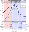 |
Fig. B.1. The features of single star models in grid CC-S at the end of the run. The middle panel shows the final mass (black), He-core mass (blue) and CO-core mass (green). The bottom panel shows the surface composition (solid lines, left axis) and the central C abundance at core He-depletion (dotted line, right axis). The top panel highlights the models that are expected to implode (black background), for different explodability criteria. Background colors show the expected evolutionary outcome of a model in that mass range, either WD (white), Type IIP/L (red), Type IIb (green) or Type Ibc supernova (blue). |
The progenitors of Type Ibc supernovae show varying masses distributed around two clearly distinct peaks. About 78% of Ibc progenitors have Mej = 11.3 − 13.3 M⊙ and the remaining 22% around 3.8 − 6.5 M⊙. The second peak originates from the very massive stars at ZAMS (Mi > 65 M⊙, cf. Fig. B.1) that show severe mass-loss during the main-sequence. This is caused by the star showing strong He-enhancement early on in the main-sequence, which increases the mass-loss rate significantly and leads to the development of a smaller core. The number of BHs formed is about 8 per 100 supernovae, with masses MBH = 10.3 − 14.2 M⊙.
When using the explodability criteria from E16 and PS20, the number of implosions increase, and the number of BHs formed significantly increases to ∼20 and ∼72 per 100 supernovae respectively. Figure B.1 shows the initial mass ranges that are mostly affected by implosions. Type IIb and Type Ibc supernovae are affected the most as many of their progenitors implode. For Type IIP/L, the only progenitors that implode are the most massive. The relative fractions of supernovae change, generally by increasing Type IIP/L at the expense of the other supernovae. The criterion from E16 implodes some of the higher-mass Type Ibc progenitors, yielding fractions of Type IIP/L, IIb and Ibc of 85.2%, 4.7% and 10.1% respectively (and a Type Ibc to Type IIP/L ratio of 0.12), while the criterion from PS20 implodes almost all progenitors but those of Type IIP/L with MZAMS ≲ 15 M⊙.
While one cannot provide IMF-weighted distributions concerning single He-stars, we can nonetheless discuss the main trends that our models show in terms of their explodability (see Fig. B.2). The criterion from M16 predicts implosions for models with Mpre − SN ∼ 6.3 M⊙, ∼8.1 M⊙, 9 − 10 M⊙ and for > 13.1 M⊙. With the criterion from E16, additional imploding models are found with final masses between 6.9 M⊙ and 10.4 M⊙, while that of PS20 includes most models with Mpre − SN > 5.9 M⊙ and a few low-mass ones around 4.2 − 4.7 M⊙.
Appendix C: Extrapolating Case BB RLOF
The models in EJLD25 provide significant correlations between the information available before core-He depletion and the outcome of Case BB RLOF (see Appendix B in EJLD25). For this, we need to know the maximum extent in mass of the convective core during core-He burning Mconv, Hemax, the Roche-lobe radius at core-He depletion RRL, 1 and a single-star model with the same Mconv, Hemax. Therefore, we can use the single He star model and RRL, 1 to derive the time before core-collapse where this He-star would fill its Roche-lobe ΔtRLOF − BB. We calculate this value for the models shown in EJLD25 (using the He-stars in the same work) and plot their ΔMRLOF − BB against ΔtRLOF (Fig. C.1).
We constructed a fitting function that provides a good approximation to the behavior seen in the models,
![Mathematical equation: $$ \begin{aligned} \Delta M_{\rm RLOF-BB}(\Delta t_{\rm RLOF-BB}) = M_0\left(1-\mathrm{e} ^{-\left[{\Delta t_{\rm RLOF-BB}}/{\tau }\right]^\gamma }\right), \end{aligned} $$](/articles/aa/full_html/2026/02/aa57572-25/aa57572-25-eq6.gif) (C.1)
(C.1)
where M0 gives the maximum mass-loss, τ a characteristic timescale and γ a power-exponent. With our fit, we obtain a relatively good agreement with the models, with relatively limited residuals of up to 0.1 M⊙ in the low ΔtRLOF − BB regime.
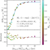 |
Fig. C.1. Fit of ΔMRLOF − BB from the models in EJLD25 as a function of the time between the onset of Case BB RLOF and core-collapse (see text). Each model is color-coded by the mass at core helium depletion MHe − dep. The fitting function and parameters are shown in the top panel. The bottom panel shows the residuals. |
Appendix D: Example of the effects of binary interaction
Binary evolution influences the evolution of the primary star by removing its hydrogen-rich envelope prior to the end of its life. Conversely, this process can help produce more massive progenitors via accretion or mergers. In Fig. D.1 we illustrate how varying initial orbital configurations lead to distinct levels of stripping, consequently resulting in diverse supernova types for a primary star of M1, i = 12.6 M⊙ (which, if isolated, would evolve to become a Type IIP/L supernova).
The tightest binaries undergo mass-transfer during the main-sequence (Case A RLOF, Pols 1994; Sen et al. 2022). Systems with Pi ≲ 2 d mostly develop into contact systems that undergo L2-outflows and thus merge (Menon et al. 2021). Some of these mergers are so massive that they are then expected to produce BHs instead of exploding as a supernova. For those systems with Pi ∼ 2 − 4 d, models undergo stable Case A only for 0.50 ≲ qi ≲ 0.85, which is followed by subsequent phases of RLOF and wind mass-loss to strip the star so severely that it will turn into a WD. For lower qi, Case A turns unstable, while for higher qi the companion stars evolve quickly enough to the point that they initiate inverse mass-transfer, which is assumed to end up in a merger (see Sect. 2.1.2). Such mergers typically produce Type IIP/L supernovae, but in some cases also give rise to Type IIb supernovae (due to the small amount of H-rich envelope that was left), and in one model this occurs so late that core-collapse may soon follow, leading to a Type IIn supernova.
For wider binaries, with 4 d ≲ Pi ≲ 1 700 d, the first phase of mass transfer occurs after the end of the main-sequence and before the beginning of core He burning (Case B RLOF). Mass-transfer efficiently removes a significant part of the H-rich envelope of the primary star, to the point that for Pi < 400 d the subsequent winds are able to remove the remaining portion of the H-rich envelope, producing Type Ibc supernova progenitors. Additionally, there is a significant parameter space for stripped He-star progenitors to expand once again and undergo Case BB RLOF, becoming progenitors of Type Ibn supernovae. For wider orbits, mass-transfer and wind mass-loss are not strong enough to remove the whole envelope, and the primary will explode as a Type IIb supernova.
For 1 000 ≲ Pi ≲ 2 500 d, the orbit is wide enough that RLOF can occur after core-He depletion (Case C mass transfer), which will lead to a Type IIn supernova (see Sect. 2.3). This also applies to models that first underwent Case B RLOF but retained massive envelopes (EJLD24). For even wider binaries (Pi ≳ 2 500 d), no mass-transfer occurs and therefore the primary star evolves as a single-star, which will then explode as a Type IIP/L supernova. This behavior is similar for different masses, although the supernova types differ.
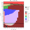 |
Fig. D.1. Expected evolutionary outcome for the primary star, or merger product, for each model in the binary grid with M1, i = 12.6 M⊙ shown in the log Pi − qi diagram. The explodability criterion used is that of M16 and the mergers are given by the hard-coded criteria. Models that undergo unstable RLOF are shown with hatches, and we differentiate between the case in which the donor is the primary star (black) or the secondary star (white). Different colors represent different evolutionary outcomes (see legend). The lines in the plots separate Case A and Case B systems (dashed), Case B and Case C systems (dotted), and systems that undergo RLOF and those that do not (solid). |
Appendix E: Comparison to other theoretical predictions
Works like Eldridge et al. (2008) and Souropanis et al. (2025) discuss the relative population of Type Ibc to Type IIP/L supernovae from theoretical models accounting for single-star and binary evolution across different metallicities. In Eldridge et al. (2008), similar-metallicity models to our own result in Type Ibc to Type IIP/L ratios of ∼0.3, compared to our value of 0.48, as they neglect rotation, which can boost the appearance of H-free supernovae (e.g., Meynet & Maeder 2005). The models from Souropanis et al. (2025), also predict a similar ratio, although their models use a smaller binary fraction (fB = 60%), which also reduces their number of Type Ibc.
We also compare the results from Zapartas et al. (2019) with a similar fB to our own and find a qualitatively similar ratio of Type Ibc to Type IIP/L (∼0.39). This work also extensively focused on the progenitor channels for Type IIP/L supernovae, where they find that only 35% of Type IIP/L progenitors come from single and effectively-single stars, 20% from donors and accretors, while the remaining 45% from mergers. This is in line with our models, where we obtain respectively 37%, 23% and 40%.
The recent work by Gilkis et al. (2025) offers a more systematic comparison of different supernova types for the models at the same metallicity. They find about 67% Type IIP/L supernovae (MH, env > 0.03), 18.3% for Type IIb (where 0.030 < MH, env/M⊙ < 0.001) and 14.6% of Type Ibc supernovae. Their models produce significantly more Type IIb supernovae than our models due to the different wind recipe adopted for lower-mass partially-stripped stars (Vink 2017). However, their number of Type Ibc supernovae are in tension with those in Graur et al. (2017), which our models better replicate, while they are within 5% of the estimate from Ma et al. (2025b). The number of BHs they produce is also a factor four higher than our models (assuming the criterion from M16, which they also adopt), which can be explained by the generally higher masses that their stars show due to the weaker winds. Finally, the authors also observe an enhancement in mass-loss rates for stripped stars as they advance through their later evolutionary phases, attributed to the formation of optically-thick winds. This aspect is absent in our models, due to the divergent wind schemes adopted.
Type IIn supernovae have been investigated in Schneider et al. (2025a) using detailed single-star models to mimic the evolution of accretors and mergers in binary systems until core-collapse (Schneider et al. 2024). They assume that Type IIn supernovae are formed when the star explodes while located above the Humphrey-Davidson limit (Humphreys & Davidson 1979) and cooler than the sDor instability strip (Smith et al. 2004), under the assumption that a star in this region would show significant mass-loss prior to the explosion. While we cannot assess the evolution of merger models in the HRD, we have some secondary stars that do reach core-collapse while located in this region (see Fig.5 in Jin et al. 2025) which contribute to about 0.3% of all core-collapse supernovae. Even if they were to become Type IIn supernovae, our overall results would not be significantly affected.
The only study released so far with regards to the population of Type Ibn supernovae is from Ko et al. (2025), where the authors use a population synthesis code (Kinugawa et al. 2014, 2016, 2024) to produce the population of these transients through mass-transfer with a main-sequence star or compact-object. They find that their Type Ibn supernovae account for 1 − 3% of all supernovae, with > 85% of them coming from He-stars transferring mass to a secondary main-sequence star (see their Fig.4). Their results are not only compatible with our results, but also justify our assumption of exclusively studying the primary-star progenitors for Type Ibn supernovae.
Appendix F: Ratios
Figure F.1 shows complementary information to Fig. 8 including the number of BHs and the ratios of different supernova types.
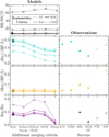 |
Fig. F.1. As Fig. 8 but showing ratios between transients or BHs formed. We show the ratio of BHs to supernovae (top left, in percent), Type Ibc to Type IIP/L supernovae (bottom left), Type IIn to Type IIP/L (top right) and Type Ibn to Type Ibc (bottom right). |
All Tables
All Figures
|
Fig. 1. Pie charts of the distribution of supernova types (different colors) from the models assuming the explodability criterion of M16 and the hard-coded merger criteria. The contribution from stars that do not undergo mass transfer is marked with a white hatching. The four lower panels represent the contribution from each progenitor type (primary and secondary stars that were affected by mass transfer, merger products, and single and effectively single stars). The contribution of each channel is given in the center of the respective pie. The legends show the contribution to each supernova type to the whole distribution. We show a comparable plot based on the explodability criteria of PS20 in Fig. 6. |
| In the text | |
|
Fig. 2. Stacked histograms of the ejecta mass Mej in our fiducial population model grouped by the supernova type (Type IIP/L, IIb, and Type Ibc supernovae) and normalized by the total number of supernovae (in percent). The contribution is split between primary stars (teal), secondary stars (magenta), merger products (dark gold) or single and effectively single stars (gray). The contribution from stars that have not undergone mass transfer is hatched. The pie charts show the relative contribution of different progenitors to each supernova type. The legend also shows the fraction of supernovae within the whole distribution, and their sum is reported inside the pie charts. Separately, we show a histogram for the mass of BHs, with a pie chart showing the relative contribution of different progenitors, and the number is normalized to that of supernovae. Less than one percentile of the distribution of Type IIP/L supernovae and BHs falls outside of the shown ranges, extending up to 43 M⊙. We show a comparable plot based on the explodability criteria of PS20 in Fig. 7. |
| In the text | |
|
Fig. 3. Ejecta masses Mej vs. CSM masses MCSM of our Type IIn supernova progenitors (main panel). The right and upper panels show the MCSM and Mej histograms. The lines in the scatter plot indicate constant fM (Eq. 2), which represents the conversion efficiency of the ejecta kinetic energy into radiation as it impacts the CSM, assuming spherical symmetry. We distinguish the contribution from models undergoing stable Case C (filled orange), unstable Case C (filled blue), and Case C following Case B (empty orange). The inferred properties from a sample of observed Type IIn supernovae from Ransome & Villar (2025) is also shown (gray dots). |
| In the text | |
|
Fig. 4. Comparison of the distribution of the integrated bolometric light-curve luminosity Erad of observed Type IIn supernovae (top) and the conversion efficiency fM from our models (bottom). The data from Hiramatsu et al. (2024) distinguish between a high-luminosity group (Erad ∼ 1.8 × 1050 erg, blue) and a low-luminosity group (Erad ∼ 1.4 × 1049 erg, orange), while that of Ransome & Villar (2025) is derived via MOSFIT by fitting and integrating the bolometric light curve for each transient until day 200 after the explosion. The data from Ransome & Villar (2025) were normalized to the total number of transients they analyzed. |
| In the text | |
|
Fig. 5. Same diagram as in Fig. 3 for Type Ibn progenitors. We include the inferred properties of the observed Type Ibn previously collected by EJLD25 (see references therein, blue circles) including more recent ones from Wang et al. (2025) (i.e., SN2020nxt, 2020tax, SN2021bbv, SN2023utc, and SN2024aej). In the top right corner, we show a histogram of fM. |
| In the text | |
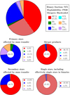 |
Fig. 6. As Fig. 1, but assuming the explodability criteria of PS20. |
| In the text | |
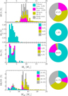 |
Fig. 7. As Fig. 2, but assuming the explodability criteria of PS20. |
| In the text | |
|
Fig. 8. Comparison between the predictions on the fractions of supernovae of different types (different blocks) produced by the models (left subpanel, with our supernova nomenclature on the left y-axis) and the observed fractions (right subpanel, with the observed subtypes that we clumped in each group on the right y-axis). The numbers are reported as a fraction of all core-collapse supernovae. For the models, a line plot show the variation of the fraction of supernovae subtypes as a function of different merger criteria added on top of the hard-coded criteria (‘None’ on the x-axis), sorted from left to right by those that produce less to more mergers that reach core collapse (see text). Different dashes shows the same while assuming different explodability criteria sorted by increasing number of implosions, that all stars successfully explode (All), Müller et al. (2016, M16), Ertl et al. (2016, E16), and Patton & Sukhbold (2020, PS20). The star corresponds to the fiducial model. For the observation, we show the estimates from volume-limited samples from Eldridge et al. 2013 (E13), the LOSS survey (specifically, the subsample from high-mass galaxies, which serves as a proxy of high-metallicity environments; Graur et al. 2017), and the samples from Ma et al. 2025b (M25) and ASAS-SN (Pessi et al. 2025) with filled markers. We also include for reference the magnitude-limited samples from PTF (Schulze et al. 2021) and ZTF (Hinds et al. 2025), shown with empty markers. |
| In the text | |
|
Fig. B.1. The features of single star models in grid CC-S at the end of the run. The middle panel shows the final mass (black), He-core mass (blue) and CO-core mass (green). The bottom panel shows the surface composition (solid lines, left axis) and the central C abundance at core He-depletion (dotted line, right axis). The top panel highlights the models that are expected to implode (black background), for different explodability criteria. Background colors show the expected evolutionary outcome of a model in that mass range, either WD (white), Type IIP/L (red), Type IIb (green) or Type Ibc supernova (blue). |
| In the text | |
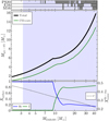 |
Fig. B.2. As Fig. B.1 but for single He-star models in grid CC-He. |
| In the text | |
|
Fig. C.1. Fit of ΔMRLOF − BB from the models in EJLD25 as a function of the time between the onset of Case BB RLOF and core-collapse (see text). Each model is color-coded by the mass at core helium depletion MHe − dep. The fitting function and parameters are shown in the top panel. The bottom panel shows the residuals. |
| In the text | |
|
Fig. D.1. Expected evolutionary outcome for the primary star, or merger product, for each model in the binary grid with M1, i = 12.6 M⊙ shown in the log Pi − qi diagram. The explodability criterion used is that of M16 and the mergers are given by the hard-coded criteria. Models that undergo unstable RLOF are shown with hatches, and we differentiate between the case in which the donor is the primary star (black) or the secondary star (white). Different colors represent different evolutionary outcomes (see legend). The lines in the plots separate Case A and Case B systems (dashed), Case B and Case C systems (dotted), and systems that undergo RLOF and those that do not (solid). |
| In the text | |
|
Fig. F.1. As Fig. 8 but showing ratios between transients or BHs formed. We show the ratio of BHs to supernovae (top left, in percent), Type Ibc to Type IIP/L supernovae (bottom left), Type IIn to Type IIP/L (top right) and Type Ibn to Type Ibc (bottom right). |
| In the text | |
Current usage metrics show cumulative count of Article Views (full-text article views including HTML views, PDF and ePub downloads, according to the available data) and Abstracts Views on Vision4Press platform.
Data correspond to usage on the plateform after 2015. The current usage metrics is available 48-96 hours after online publication and is updated daily on week days.
Initial download of the metrics may take a while.