| Issue |
A&A
Volume 706, February 2026
|
|
|---|---|---|
| Article Number | A280 | |
| Number of page(s) | 21 | |
| Section | Interstellar and circumstellar matter | |
| DOI | https://doi.org/10.1051/0004-6361/202558059 | |
| Published online | 18 February 2026 | |
Exploring the interplay between molecular and ionized gas in H II regions
1
Max-Planck-Institut für Radioastronomie,
Auf dem Hügel 69,
53121
Bonn,
Germany
2
I. Physikalisches Institut, Universität zu Köln,
Zülpicher Str. 77,
50937
Köln,
Germany
3
Deutsches Zentrum für Astrophysik,
Postplatz 1,
02826
Görlitz,
Germany
4
National Radio Astronomy Observatory,
PO Box O, 1003 Lopezville Road,
Socorro,
NM
87801,
USA
5
Centre for Astrophysics and Planetary Science, University of Kent,
Canterbury
CT2 7NH,
UK
6
Department of Earth & Space Sciences, Indian Institute of Space Science and Technology,
Trivandrum
695547,
India
7
Purple Mountain Observatory, and Key Laboratory of Radio Astronomy, Chinese Academy of Sciences,
10 Yuanhua Road,
Nanjing
210023,
PR
China
★★ Corresponding author: This email address is being protected from spambots. You need JavaScript enabled to view it.
Received:
11
November
2025
Accepted:
18
December
2025
Abstract
Context. Massive stars strongly impact their natal environments and influence subsequent star formation through feedback mechanisms such as shocks, outflows, and radiation. H II regions are key laboratories for studying this impact. To understand such feedback, it is crucial to characterize the physical conditions of the dense molecular gas in which these regions are embedded.
Aims. We aim to constrain the kinetic temperature and H2 volume density of massive star-forming clumps associated with H II regions using multiple p–H2CO transitions. In addition, we investigate the interplay between ionized gas, molecular gas, and dust to probe how massive stars influence their parental clumps.
Methods. We observed the JKaKc transitions of p–H2CO (within its J = 3–2 and 4–3 states) with the Atacama Pathfinder EXperiment (APEX) 12 m submillimeter telescope, using the nFLASH230 and SEPIA345 receivers toward a sample of 61 H II regions. We derived spectral line parameters via multicomponent Gaussian fitting, which was then used to constrain the physical conditions determined using PyRADEX, a non–local thermodynamic equilibrium (LTE) radiative transfer code in combination with Markov chain Monte Carlo analysis.
Results. The non-LTE analysis yielded kinetic temperatures (Tkin) ranging from 33.7 K to 265 K and H2 densities (n(H2)) between 0.8 × 10⁴ and 1.05 × 107 cm−3, providing a detailed characterization of the dense molecular gas contained in these clumps. In addition to the p–H2CO emission arising from the targeted clump, a large fraction (57%) of the sources exhibited multiple p–H2CO components, with the secondary components being characterized by a higher Tkin and broader line widths. Investigation of the nature of the secondary component revealed its association with supersonic nonthermal motions and turbulent gas. When comparing the physical properties of the molecular gas and dust components with those of the ionized gas, we found that parameters directly linked to the central high-mass star, such as bolometric luminosity (Lbol) and Lyman continuum photon rate (NLyc), show stronger and more systematic correlations. These findings emphasize the role of the central star in governing the interplay between the molecular and ionized gas. In our sample of H II regions, the pressure of the neutral gas systematically exceeds that of the ionized gas. This suggests that the surrounding neutral molecular medium can hinder or slow down the expansion of H II regions due to its higher pressure. However, given the limited spatial resolution, a definitive conclusion on the role of molecular gas in confining H II regions cannot be made until high resolution observations are obtained.
Key words: stars: formation / stars: massive / ISM: clouds / HII regions / ISM: molecules
Member of the International Max Planck Research School (IMPRS) for Astronomy and Astrophysics at the Universities of Bonn and Cologne.
Deceased.
© The Authors 2026
 Open Access article, published by EDP Sciences, under the terms of the Creative Commons Attribution License (https://creativecommons.org/licenses/by/4.0), which permits unrestricted use, distribution, and reproduction in any medium, provided the original work is properly cited.
This article is published in open access under the Subscribe to Open model.
Open Access funding provided by Max Planck Society.
1 Introduction
High-mass stars (>8 M⊙) are fundamental drivers of galactic evolution and dynamics through their strong interaction with the surrounding interstellar medium (ISM). These stars play a crucial role in regulating the Galaxy’s energy balance through feedback mechanisms such as strong stellar winds, the intense ionizing ultraviolet (UV) radiation throughout their lifetimes, and the powerful supernova explosions at the end of their life cycles. The UV photons emitted by high-mass stars have enough energy to ionize the surrounding neutral hydrogen, resulting in the formation of H II regions. Because these stars have short lifetimes – only a few million years (see Motte et al. 2018, and reference therein) – and are deeply embedded in their natal molecular clouds, H II regions observed via their radio free-free emission or radio recombination lines (RRLs) serve as strong indicators of recent high-mass star formation (HMSF) activity in the Galaxy.
As H II regions evolve, they expand under the combined influence of internal pressure, stellar radiation, and winds from central OB stars. This expansion can compress the surrounding molecular gas, potentially triggering secondary star formation along the ionization fronts (Deharveng et al. 2010; Elmegreen 2011; Thompson et al. 2012). Young embedded H II regions profoundly affect their environments through feedback mechanisms such as shocks, outflows, and radiation, thereby shaping the conditions for subsequent star formation (Elmegreen & Lada 1977; Deharveng et al. 2003; Elmegreen 2011). However, the extent to which these regions modify the initial conditions or trigger new episodes of HMSF within their parental molecular clouds remains uncertain. A comprehensive understanding of these processes requires accurate measurements of the molecular gas temperature and density near expanding H II regions, along with the physical characteristics of the associated ionized gas and the relationships between them.
Previous extensive radio continuum and recombination-line surveys have unveiled a large number of Galactic H II regions (e.g., Reifenstein et al. 1970; Altenhoff et al. 1979; Lockman 1989; Kuchar & Clark 1997; Urquhart et al. 2007, 2009, 2013; Anderson et al. 2011, 2014; Kalcheva et al. 2018; Gao et al. 2019). Recently, the GLObal view on STAR Formation in the Milky Way survey (GLOSTAR1; Medina et al. 2019; Brunthaler et al. 2021) cataloged a large population of new and known H II regions using highly sensitive Karl G. Jansky Very Large Array (VLA) continuum data in the D (Medina et al. 2019, 2024) and B configuration (Dzib et al. 2023; Yang et al. 2023) at spatial resolutions of 18″ and 1″, respectively. Khan et al. (2024, hereafter Paper I), compiled a catalog of Galactic H II regions detected with GLOSTAR RRLs data observed with the VLA in the D configuration and analyzed their ionized gas properties. This study revealed that approximately 50% of these H II regions are associated with sources identified in the Atacama Pathfinder EXperiment (APEX) Telescope Large Area Survey of the GALaxy (ATLASGAL; Schuller et al. 2009), which provided a comprehensive view of HMSF at 870 μm – a wavelength particularly sensitive to cold dust emission tracing dense star-forming clumps. While the ATLASGAL survey determined properties of the dust, the gas density and temperature of the clump play a crucial role in regulating their chemistry and star formation activity as well as in influencing the stellar initial mass function. A precise measurement of the dense gas density and temperature in the vicinity of the H II region are essential to deepening our understanding of how H II regions impact their parental molecular clouds and surrounding environments.
H2CO, which has been ubiquitously detected in the ISM, is primarily formed via the hydrogenation of CO on dust grain surfaces (Simons et al. 2020) and is subsequently released into the gas phase through processes such as UV irradiation or shocks. As a result, it is commonly associated with star-forming and H II regions (Downes et al. 1980; Henkel et al. 1983; Du et al. 2011; Ginsburg et al. 2011; Gong et al. 2023), where its abundance remains relatively stable throughout different stages of the star formation cycle (Mangum et al. 1990; Tang et al. 2018b). Due to its large dipole moment (2.33 Debye; Fabricant et al. 1977), H2CO exhibits rotational transitions across the centimeter and submillimeter wavelength range (Mangum & Wootten 1993). Spectroscopically, the rotational states of this asymmetric and prolate molecule are described by the total angular momentum and its projection quantum numbers, JKaKc. Furthermore, due to the nuclear spin of the hydrogen nuclei, H2CO exists in two spin isomers: ortho (Ka = odd) and para (Ka = even). However, one of the most valuable properties of H2CO for astrophysical studies is its characteristic “K-doublet” splitting, which arises from the coupling between vibrational and rotational angular momentum states. In its rotational spectrum, this results in closely spaced pairs of spectral lines (or “K-doublets”) with opposite parity, rather than a single transition.
With advancements in receiver technology and increased access to submillimeter windows, astronomers have expanded the utility of H2CO as a diagnostic tool for characterizing the physical conditions in molecular gas, even using its higher lying submillimeter transitions (Tang et al. 2018a,b, 2021, and references therein). These properties make H2CO one of the very few molecular species that act as both a thermometer and densitometer for dense gas, particularly in environments where other tracers such as NH3 or CH3CN may be less accessible. For these reasons observations of the “K-doublet” transitions of H2CO serve as a great tool to study the physical properties of the molecular medium and allow observations with a variety of radio telescopes.
To summarize, detailed study of a large sample of embedded H II regions and surrounding molecular clouds is required to probe the underlying physical processes, the physical properties of the ambient dense molecular cloud into which they are expanding, and the effect of HMSF on the parent molecular clouds. To measure the kinetic temperature and gas density of massive star-forming clumps identified in the GLOSTAR H II region and ATLASGAL surveys, here we analyze the rotational transitions of p–H2CO (J = 3–2 and 4–3). Using these results, we aim to (a) explore possible correlations between the characteristics of molecular gas, ionized gas, and dust in these regions; (b) examine the temperature and density structure of molecular gas surrounding H II regions; and (c) investigate whether the pressure of the surrounding medium is sufficient to confine H II regions. This paper is structured as follows: In Sect. 2, we describe the source sample studied, the selection criteria we used, the H2CO observations, and data reduction process. In Sect. 3, we outline the methods used to analyze and model the observed spectral line profiles of the p–H2CO transitions studied. Section 4 presents the results, and this is followed by a discussion in Sect. 5. Finally the main conclusions are summarized in Sect. 6.
2 Sample, observations, and data reduction
2.1 Source selection
We identified 244 Galactic H II regions in Paper I using detected stacked RRLs (H98α–H114α) within the GLOSTAR survey coverage (−2° ≤ ℓ ≤ 60° & |b| ≤ 1° and 76° ≤ ℓ ≤ 83° & −1° ≤ b ≤ 2°). These authors derived physical properties of identified H II regions such as the electron temperature, electron density, and emission measure to characterize the associated ionized gas. By comparing the H II region catalog with dust continuum data, it was found that nearly half of the identified H II regions are spatially associated with dust clumps from the ATLASGAL survey. Urquhart et al. (2018, 2022) previously classified these clumps as H II regions and provided key dust properties such as the bolometric luminosities (Lbol), the clump masses (Mclump), and the dust temperatures (Tdust). Such a combined dataset offers insights into both the ionized gas and dust components associated with H II regions. This study extends the analysis in Paper I by investigating in addition to the ionized gas and dust, the properties of the molecular gas surrounding H II regions and exploring their interplay.
The targets for this study were selected based on the following criteria: (1) the ionized gas properties of the H II regions have already been derived (as cataloged in Paper I); (2) the target has an association with 870 μm continuum emission taken from ATLASGAL catalog, with dust properties derived in Urquhart et al. (2018, 2022); (3) the deconvolved full width half maximum (FWHM) of the H II region (from Paper I) is comparable to or smaller than that of the corresponding ATLASGAL clump; and (4) the target has well-characterized kinematics. We excluded H II regions located toward the Galactic center (−2° ≤ ℓ ≤ 2°) and the Cygnus X complex due to significant uncertainties in their kinematic distances.
These criteria ensure that the targeted H II regions are likely to remain embedded within their natal molecular clouds, enabling an investigation of the physical link between the ionized and molecular components during massive star formation. Based on these criteria, we selected 61 H II regions from Paper I for the p–H2CO spectral line observations. Figure A.1 presents three–color mid–infrared composite images (8,24, and 70 μm) with contours marking the GLOSTAR 5 GHz radio continuum emission, highlighting the selected H II regions in this study.
Among them, only G30.720–0.082 is unresolved in the GLOSTAR RRL data at 25″ resolution (see Fig. A.2). Six sources (G7.177+0.088, G10.440+0.011, G24.470+0.490, G25.159+0.060, G43.169+0.008, and G43.149+0.013) exhibit extended radio emission surrounding compact bright cores, resulting in sizes larger than their associated ATLASGAL clumps (see Fig. A.2). We retained these sources in the sample to preserve diversity in the population. The selected regions span Galactic longitudes from 3° ≤ ℓ ≤ 53°, encompassing several prominent high-mass star-forming complexes, including W31, W33, W43, and W51.
Figure 1 presents the Galactic distribution of the sources in this study, overlaid on an artist’s impression of the Milky Way2. The sources span distances from 1.8 to 20.4 kpc, with values for each H II region and its associated clump taken from Paper I (and references therein). The distribution reveals two distinct populations: one clustered near 4 kpc and another around 12 kpc. Figure A.3 shows the distributions of the angular and physical sizes of the selected H II regions. The angular sizes are concentrated, with a median of 15.6", reflecting our selection criterion based on source angular size. The physical size distribution, with a median of 0.52 pc, is more scattered, due to scatter in distance. This scatter in distance introduces no significant bias in the H II region properties but rather ensures a diverse and representative sample in terms of size and spectral type of central OB stars of H II region as discussed in Appendix B.
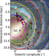 |
Fig. 1 Galactic distribution of the source sample. The locations of the targets are denoted by red stars on an artistic rendering of the Milky Way. The distances to the observed H II regions and their associated clumps are taken from Paper I (and references therein). The spiral arms are marked following the description presented in Reid et al. (2019), and the individual spiral arms are colored as follows: the 3 kpc in magenta, the Norma-Outer Arm in red, the Scutum-Centaurus Arm in blue, the Sagittarius-Carina Arm in green, the Local Arm in cyan, and the Perseus Arm is in yellow. |
2.2 APEX 12 m observations of H2CO
The single pointing observations were carried out from March to April 2023 using the Atacama Pathfinder EXperiment (APEX; Güsten et al. 2006)3 12 m submillimeter telescope located in the Chajnantor plateau, Chile. Table 1 summarizes the key spectroscopic parameters of the observed p–H2CO transitions alongside the receiver setups used and the detection rates within the sample. All three transitions of p–H2CO within the J=3–2 states near 218 GHz were observed using the dual sideband nFLASH230 receiver. At this frequency, the observations were carried out with a half-power beam width of ~27″. In addition to these p–H2CO transitions, the receiver was tuned such that it also covered the H30α line at 231 GHz in its upper sideband. Total integration times between 7 min and 16 min were spent in this setup. The nFLASH230 receiver was connected to a MPIfR-built high-capacity fast Fourier transform spectrometer (FFTS; Klein et al. 2012) backend with two sidebands. Each sideband has two spectral windows with 4 GHz bandwidth, providing both orthogonal polarizations and resulting in a total bandwidth of 8 GHz. This provided a spectral resolution of 61 kHz, resulting in a velocity resolution of 0.08 km s−1 at 218 GHz.
The three transitions of p–H2CO within the J=4–3 levels were observed with the SEPIA345 receiver (Meledin et al. 2022) with a beam size of ~20″ and integration times between 8 min to 20 mins. Similar to the nFLASH230 receiver, the SEPIA345 receiver is a dual polarization, dual sideband receiver which covers a total frequency range from 272 GHz to 376 GHz. Each sideband (and polarization) of the SEPIA345 receiver output is recorded using two FFTS spectrometer units, each of them sampling 4 GHz, with a spectral resolution of up to 64 k channels per sideband, this results in velocity resolutions of 0.04 km s−1. Both sets of observations were performed in position-switching mode with off positions offset from the on position of the sources by (±600″, ±600″) in (ℓ, b).
The data reduction was performed using the CLASS software from the GILDAS package4. The spectra were converted from antenna temperature (TA) scales to main-beam brightness temperature (TMB) scales using a factor of ηF/ηMB, where ηF is the forward efficiency and ηMB5 is the telescope main beam efficiency. In our observations, ηF was set to 0.95 and ηMB = 0.79 ± 0.07 for the data collected using both nFLASH230 and SEPIA354 (based on observations of Mars). To enhance the signal-to-noise ratios (S/N) in individual channels for both sets of observations, the data were smoothed to a uniform channel spacing of 0.6 km s−1. The typical line width of H2CO transitions toward H II regions tends to be on the order of a few kilometer per second, so the channel smoothing has no adverse impact on our results.
Summary of the p–H2CO transitions observed in this study.
3 Analysis
In this section, we describe the multicomponent Gaussian fitting of the p–H2CO spectral lines observed in this study. We then use the resulting line-fitting parameters to constrain the non-local thermodynamic equilibrium (non-LTE) analysis and derive the kinetic temperature (Tkin), gas density n(H2), and the p–H2CO column density N(p–H2CO).
3.1 Spectral line fitting
We modeled the observed spectral line features using Gaussian profiles that were fit using the MODEL function within the LMFIT6 package in Python. As output, it provided the velocity-integrated line intensity (I = ∫ Tmbdv), the local standard of rest (LSR) velocity (vLSR), the FWHM of the Gaussian line, and the peak brightness temperature on main-beam temperature scales (Tpeak).
We began our analysis by fitting single-component Gaussian to the p–H2CO spectra. However, this approach yields well constrained physical parameters for only 25 out of 61 targets (40%). To improve the modeling, we performed multicomponent Gaussian fits to better model the observed p–H2CO line profiles. As the brightest transition, p–H2CO (30,3–20,2) was detected toward all sources and served as the reference for identifying the number of velocity components and their centroid velocities. These centroid velocities were then fixed for all other p–H2CO transitions to ensure consistency across lines. Each p–H2CO (30,3–20,2) spectrum was initially fit with one Gaussian component, if the residuals are larger than 3σ, a second or even a third component was added, until the standard deviation in the residual is minimized. We verified all fits interactively using the LINE/MINIMIZE task in CLASS/GILDAS. To verify that the H2CO lines exhibit multiple components and are not affected by optical depth effects such as self-absorption, we compared their spectra with those of the optically thin C18O line. We did not find any evidence of self-absorption in our sample. We found no preferential occurrence of multiple components in sources located at either near or far distances.
Among the 61 observed sources, the p–H2CO spectra toward 34 of them displayed multiple Gaussian components, resulting in a total of 105 identified components in the entire sample. Since all six transitions are expected to trace gas with similar kinetic temperature and dynamic motion, we expect them to have similar line widths. However, this need not always be true especially when fitting additional components arising from surrounding envelopes or outflows. Therefore, the line widths were allowed to vary within 1 σ of the value constrained by the line width of the 30,3–20,2 line of p–H2CO, whereas the velocity centroids of the components were fixed. Any component with peak brightness temperatures below 3σ level of the rms noise at 0.6 km s−1 or line width less than 3×Δv (1.8 km s−1), is flagged before further analysis. An example of the p–H2CO multicomponent Gaussian fitting is shown in Fig. 2 (left panel) toward one of the targets in our study, AGAL045.121+00.131 (also listed as G045.122+0.131 in the GLOSTAR H II region catalog).
If a source exhibits multiple velocity components, then the component associated with the source at a p–H2CO velocity close to the systemic velocity of the corresponding ATLASGAL clump – determined from multiple molecular line surveys and reported by Urquhart et al. (2018, see their Table 1) – is considered the main component and is hereafter referred to as “H2CO Main.” All secondary components are then considered as sub-components and is hereafter referred to as “H2CO Sub.” These secondary components may either be associated with the source itself via outflows/inflows, envelops, or may arise from distinct molecular clumps covered in our beam. However, owing to the limited spatial resolution, the exact origin of the “H2CO Sub” components remains uncertain.
The derived line parameters for p–H2CO are then used as input to constrain the column densities and the gas densities. However, as we observed two different sets of transitions (J = 3–2 and J = 4–3) at different frequencies (218 GHz and 291 GHz) using two different receivers (nFLASH230 and SEPIA345), with varying HPBWs 27.6″ and 20.7″, the observations resulted in slightly different spatial coverages. Therefore, to ensure uniformity, we further correct for beam filling effects. Previous studies of H2CO (Immer et al. 2014; Tang et al. 2018a,b) have demonstrated a tight correlation between the integrated intensities of the p–H2CO transitions and flux density of the dust emission at 870 μm. This suggests that the dense gas traced by H2CO is associated with dust emission at 870 μm. Based on these findings, we assume that the size of the H2CO emitting area toward the targets of this study are equivalent to the FWHM source sizes of 870 μm dust emission, as derived by Csengeri et al. (2014). Following Tang et al. (2018b), we corrected for beam dilution as follows, TMB/ηbf where ηbf is the beam filling factor, given by, ![Mathematical equation: $\[\eta_{\mathrm{bf}}=\theta_{\mathrm{S}}^{2} /\left(\theta_{\mathrm{S}}^{2}+\theta_{\text {beam}}^{2}\right)\]$](/articles/aa/full_html/2026/02/aa58059-25/aa58059-25-eq1.png) . Here, θS and θbeam denote the source and beam size, respectively. The corrected p–H2CO line intensities with the respective beam filling factors used and other line fitting parameters are summarized in Tables C.1 and C.2.
. Here, θS and θbeam denote the source and beam size, respectively. The corrected p–H2CO line intensities with the respective beam filling factors used and other line fitting parameters are summarized in Tables C.1 and C.2.
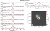 |
Fig. 2 Spectra of the different p–H2CO and RRL transitions studied in this work toward AGAL045.121+00.131. Left panels: spectra of all six of the observed p–H2CO transitions (black) along with the multicomponent Gaussian fitting (green and magenta) and residual of the fitting (dashed blue). The total fit is displayed in red and the gray shaded region demarcates the 3σ level of the rms noise. The vertical dashed gray lines mark the centroid velocities of each fit Gaussian component. Right panel: spectra of the stacked GLOSTAR ⟨Hnα⟩ RRL in black alongside the Gaussian fit in red. Also displayed is the 5.3 GHz radio continuum emission map obtained with the GLOSTAR VLA D configuration toward this source and overlaid with white contours is the ATLASGAL 870 μm. The white filled circle shows the 25″ GLOSTAR beam. |
3.2 Non-LTE modeling with Pyradex
We carried out non-LTE radiative transfer calculations to derive the physical properties of the clumps, including the gas kinetic temperature, Tkin, spatial density, n(H2), and column density of p–H2CO, N(p–H2CO). We employed the Python wrapper, PyRADEX, to interface with the non-LTE radiative transfer code RADEX (van der Tak et al. 2007), in combination with the emcee7 (Foreman-Mackey et al. 2019) package in Python, which implements a Markov chain Monte Carlo (MCMC) algorithm as shown in Yang et al. (2017) and Christensen et al. (in prep.). To reproduce the observed integrated line intensities of the varied p–H2CO transitions (as determined in the previous Sect. 3.1), the PyRADEX models were run with constraints from the observed line widths using collisional rate coefficients computed for collisions between p–H2CO and ortho-, and para-H2 (Wiesenfeld & Faure 2013) and assuming the ortho-to-para ratio (OPR) of 3. For each velocity component toward a given source, the line width was fixed to the average value across the different p–H2CO transitions probed. This approach minimizes variations and allows us to simultaneously reproduce the physical conditions traced by all six transitions – a valid constraint, since all transitions are expected to originate from the same gas. We further assumed a background temperature, Tbkg, of 2.73 K. We initialized the MCMC process using the curve_fit function from the SciPy8 package in Python, then explored the parameter space within n(H2) = 10–1010 cm−3, Tkin = 10–300 K and N(p–H2CO) = 1010–1017 cm−2. For each component, we used 400 walkers, discarding the first 100 steps as burn-in and allowing the final 1000 steps to converge on the best-fit integrated line intensity (see also Christensen et al., in prep.). Using this method, we were able to successfully constrain the physical parameters toward 83 of the 105 targets studied in this work. Figure A.4 illustrates the results of the PyRADEX and MCMC computation, displaying the results in the form of a corner plot with 1D histograms of the posterior distributions across the explored parameter space. Table C.3 lists the derived gas kinetic temperatures, volume densities, and column densities of p–H2CO. Figure 3 displays the distribution of the sources in the n(H2) − Tkin parameter space. The “H2CO Main” components of sources with single and multiple Gaussian profiles show a similar distribution, while the extreme values are associated with the “H2CO Sub” components. The only exceptions are G31.412+0.308, which exhibits the highest Tkin, and G10.462+0.033, which shows the highest n(H2).
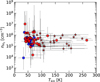 |
Fig. 3 Distribution of the sources in the n(H2)–Tkin plane. The blue and red colors respectively represent sources with single and multiple component Gaussian profiles. Filled circles denote components classified as “H2CO Main,” while stars indicate those identified as “H2CO Sub.” |
4 Results
In the following section, we present the results obtained from the joint PyRADEX and MCMC analyses described in Sect. 3.2. These results include the derived kinetic temperature, gas density, p–H2CO column density, and the fractional abundance of p–H2CO, X(p–H2CO), which we compare with values from previous studies. We also examine the optical depth of p–H2CO and assess its impact on our analysis (Appendix D).
Figure 4 shows the distributions of gas kinetic temperatures, gas densities, and p–H2CO column densities, jointly constrained from the PyRADEX and MCMC analyses discussed above while the results toward each source are listed in Table C.3. In the following sections, we discuss these results in detail.
4.1 Gas densities
As shown by the distributions in Fig. 4 for our sample, the derived n(H2) values range between 8.32 × 103 cm−3 and 1.05 × 107 cm−3 with a median9 value of (3.7 ± 0.35) × 105 cm−3. Our results are consistent with previous studies of starforming regions (Mangum & Wootten 1993; McCauley et al. 2011; Mangum et al. 2013), including the brightest ATLASGAL clumps associated with H II regions, where densities of 6.4 × 10⁵–8.1 × 106 cm−3 were reported, with a median value of 1.25 × 105 cm−3 (Tang et al. 2018b). Furthermore, a comparison of our results with n(H2) values determined from 870 μm dust emission (Urquhart et al. 2022) reveals systematically higher densities within our sample (Fig. 5), indicating that these p–H2CO transitions trace denser gas than the dust continuum. This holds true for both the systemic velocity components and additional components arising from the envelopes or other expanding shells of these H II regions. Figure 4 a shows that the median gas density of the “H2CO Sub” component similar to that of the “H2CO Main.”
4.2 Kinetic temperature
As with n(H2) and N(p–H2CO), the PyRADEX+MCMC models yielded a range of gas temperatures across the sources in our sample, from 33.7 K to >265 K10, with a median value of 66 ± 3 K. In contrast, the study by Tang et al. (2018b), which examined ATLASGAL dust clumps at various evolutionary stages, reports a median kinetic temperature of 67 K across their entire sample, increasing to 104 K for sources associated with only H II regions. To assess whether the difference in kinetic temperature derived for the H II region sample by Tang et al. (2018b) and this work are statistically significant, we applied the Anderson-Darling (AD) test to the two distributions. The resulting p-value of approximately 0.001 indicates a statistical difference between the kinetic temperature distributions, providing evidence that Tkin do not arise from the same parent population. This discrepancy in kinetic temperatures may be due to the fact that we decompose the observed spectral features into multiple components likely originating from different environments, while Tang et al. (2018b) carry out their analysis by considering only the integrated line intensities across the entire observed features. The latter may lead to higher line intensity ratios in the analysis conducted by Tang et al. (2018b), resulting in higher overall gas temperatures. Furthermore, we find the values of Tkin derived for the “H2CO Sub” components (98.4 K) to be higher than that for the “H2CO Main” components (57.8 K). This suggests that the “H2CO Sub” components may originate from inflowing/outflowing gas surrounding the star, or from shock-heated molecular gas. Moreover, the lack of correlation between the kinetic temperature of the “H2CO Sub” component and its velocity difference with both the “H2CO Main” component and the RRL emission further supports a shock-heated origin for the “H2CO Sub” components.
The Tkin values derived from the PyRADEX+MCMC analysis can be verified using the integrated intensity ratios between specific p–H2CO transitions, namely, R1 = I(321–220)/I(303–202), and R2 = I(422–321)/I(404–303) – which provide an estimate of the Tkin assuming conditions of LTE. This method is applicable if the observed lines are optically thin (discussed further in Appendix D) and originate from high-density regions. Following the approach outlined in Appendix A of Mangum & Wootten (1993), we computed the Tkin using these line ratios:
![Mathematical equation: $\[T_{\mathrm{LTE}}(R_1)=\frac{47.1}{\ln~ \left(0.556 \frac{I\left(3_{03}-2_{02}\right)}{I\left(3_{21}-2_{20}\right)}\right)} ~\mathrm{K},\]$](/articles/aa/full_html/2026/02/aa58059-25/aa58059-25-eq2.png) (1)
(1)
and
![Mathematical equation: $\[T_{\mathrm{LTE}}(R_2)=\frac{47.2}{\ln~ \left(0.750 \frac{I\left(4_{04}-3_{03}\right)}{I\left(4_{22}-3_{21}\right)}\right)} ~\mathrm{K}.\]$](/articles/aa/full_html/2026/02/aa58059-25/aa58059-25-eq3.png) (2)
(2)
In Fig. 6, we refer the temperatures derived using Eq. (1) and Eq. (2) as LTE temperatures, and find the results from both line ratios to be consistent with one another. If our assumption that the p–H2CO emission is optically thin is valid, then the kinetic temperatures obtained by this method have an uncertainty of ≲30% (Mangum & Wootten 1993). Comparisons between Tkin values derived from LTE and PyRADEX+MCMC non-LTE calculations show overall consistency, although some deviations appear at higher temperatures (Fig. 6). More interestingly, the derived values of the kinematic temperature are significantly less scattered for the “H2CO Main” velocity components than the “H2CO Sub” component. Overall, these findings reaffirm the diagnostic power of H2CO an excellent molecular thermometer.
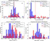 |
Fig. 4 Distributions of the pyRADEX+MCMC derived (a) n(H2), (b) Tkin, (c) N(p–H2CO), and (d) p–H2CO fractional abundance, X(p–H2CO) toward the different velocity components identified in our sample, as traced by the p–H2CO. The blue and red histograms represent the distributions for the “H2CO Main” and “H2CO Sub” components, respectively, while the corresponding dashed lines indicate the median values of each distribution. |
4.3 Fractional abundance of p–H2CO
In this section, we compute the fractional abundance of p–H2CO with respect to H2 (X(p–H2CO) = N(p–H2CO)/N(H2)), where N(H2) refers to the H2 column density derived from the 870 μm continuum emission by Urquhart et al. (2018). The PyRADEX derived N(p–H2CO) values lie between 4 × 1012 cm−2 and 5 × 1015 cm−2 with a median value of 1.0 ± 0.1 × 1014 cm−2, while N(H2) was estimated from the peak flux densities of the clumps using
![Mathematical equation: $\[N(\mathrm{H}_2)=\frac{\mathrm{D}^2 ~F_{870} ~R}{B_{870}(T_{\mathrm{d}}) ~\theta_{\text {beam}} ~\kappa_{870} \mu_{\mathrm{H}_2} ~m_{\mathrm{H}}},\]$](/articles/aa/full_html/2026/02/aa58059-25/aa58059-25-eq4.png) (3)
(3)
where D is the distance to the source; F870 is the peak flux density taken from Csengeri et al. (2014), θbeam; the beam size of ATLASGAL survey (= ![Mathematical equation: $\[19^{\prime\prime}_\cdot2\]$](/articles/aa/full_html/2026/02/aa58059-25/aa58059-25-eq5.png) ; Csengeri et al. 2014), μH2 is the mean molecular weight per hydrogen molecule assumed as 2.8, and mH the mass of the hydrogen atom. Further, R is the gas-to-dust ratio assumed to be 100; B870(Td) is the intensity of the blackbody at 870 μm at the dust temperature, Td, values for which are taken from Urquhart et al. (2018); and κ870 is the dust opacity at 870 μm taken to be 1.85 cm2 g−1, an average of all dust models presented in Ossenkopf & Henning (1994). This yields N(H2) values ranging from 6 × 1020 cm−2 to 8 × 1022 cm−2 and X(p–H2CO) values from 2.7 × 10⁻¹⁰ to 4.7 × 10⁻⁷ (see Fig. 4d), with a median value of 7.2 × 10⁻⁹. These results are consistent with values reported for other star-forming regions (Ao et al. 2013; Gerner et al. 2014; Tang et al. 2018a,b). Figure 4c shows that the median N(p–H2CO) of the “H2CO Sub” component is higher than that of the “H2CO Main”, whereas the median X(p–H2CO) is similar for both components (see Fig. 4d). This suggests that H2CO can be at least as abundant – if not more so – in the envelope/outflow components, underscoring its presence across diverse environments. However, the “H2CO Sub” components may actually represent unresolved condensates, since their densities match those of the “H2CO Main” components, suggesting that the secondary features likely comprise of multiple dense clouds at closely spaced velocities unresolved in our single dish observations.
; Csengeri et al. 2014), μH2 is the mean molecular weight per hydrogen molecule assumed as 2.8, and mH the mass of the hydrogen atom. Further, R is the gas-to-dust ratio assumed to be 100; B870(Td) is the intensity of the blackbody at 870 μm at the dust temperature, Td, values for which are taken from Urquhart et al. (2018); and κ870 is the dust opacity at 870 μm taken to be 1.85 cm2 g−1, an average of all dust models presented in Ossenkopf & Henning (1994). This yields N(H2) values ranging from 6 × 1020 cm−2 to 8 × 1022 cm−2 and X(p–H2CO) values from 2.7 × 10⁻¹⁰ to 4.7 × 10⁻⁷ (see Fig. 4d), with a median value of 7.2 × 10⁻⁹. These results are consistent with values reported for other star-forming regions (Ao et al. 2013; Gerner et al. 2014; Tang et al. 2018a,b). Figure 4c shows that the median N(p–H2CO) of the “H2CO Sub” component is higher than that of the “H2CO Main”, whereas the median X(p–H2CO) is similar for both components (see Fig. 4d). This suggests that H2CO can be at least as abundant – if not more so – in the envelope/outflow components, underscoring its presence across diverse environments. However, the “H2CO Sub” components may actually represent unresolved condensates, since their densities match those of the “H2CO Main” components, suggesting that the secondary features likely comprise of multiple dense clouds at closely spaced velocities unresolved in our single dish observations.
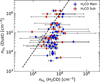 |
Fig. 5 Comparison between n(H2) probed by 870 μm emission from dust and p–H2CO as derived from our pyRADEX+MCMC models. The dashed black line displays a slope of unit value. |
5 Discussion
5.1 Correlation between physical properties of ionized gas, molecular gas, and dust
Variations in the physical properties of clumps and H II regions associated with star formation offer valuable insights into the evolutionary stages and conditions of HMSF and its impact on the surrounding medium. For instance, over the years, the ratio of bolometric luminosity to clump mass has proven to be a reliable tracer of HMSF stages and has been widely used in numerous studies (Molinari et al. 2008, 2016; Giannetti et al. 2017; Urquhart et al. 2022). Similarly, ne and RRL line widths have been extensively employed to characterize the evolutionary stages of H II regions (e.g., Sewilo et al. 2004; Kurtz 2005). In order to investigate the relationship between the ionized, molecular gas, and dust in H II regions, we compared the Spearman’s correlation between the different physical properties of molecular gas traced by p–H2CO derived in the previous sections with those of dust, and ionized gas from Paper I. The resulting correlations are presented in Fig. 7. Note that we have flagged the cross correlation for which the p-value is > 0.0013.
No strong correlation was found between n(H2) and the other ionized, molecular gas and dust properties (masked in Fig. 7). This suggests that, regardless of the specific characteristics of the HMSF clump, their molecular hydrogen densities typically remain around 105–6 cm−3, in alignment with the findings of Tang et al. (2018b).
Observations of massive clumps using other molecular line tracers such as CO, NH3, CH3CN, CH3CCH, and CH3OH, H2CO (Wienen et al. 2012; Giannetti et al. 2017; Tang et al. 2018b) suggest that these clumps are heated by radiation from embedded massive stars. This implies that the Tkin values derived from these molecules should correlate with the Lbol of the clumps. Giannetti et al. (2017) reported such correlations using kinetic temperatures derived from CH3CCH, and CH3OH, with correlation coefficients of 0.68 and 0.54, respectively. Similarly, Tang et al. (2018b) investigated the same relationship using H2CO and found a somewhat weaker correlation, with a coefficient of ~0.5. However, in this study, we find an even weaker correlation between Tkin and Lbol, with a correlation coefficient of 0.32 (masked in Fig. 7 due to p-value >0.0013).
Although the velocities of RRLs and p–H2CO lines are generally consistent, there is still a velocity offset between the two, with a standard deviation in the velocity offset of ~4 km s−1 and mean of −0.5 km s−1. For an H II region of roughly 0.52 pc in size, the inferred dynamical age is tdy ~ 1.3 × 10⁵ yr, which is comparable to the typical expansion timescales of H II regions. Hence, a clump with a velocity difference of 4 km s−1 is consistent with a molecular layer being located near the ionization front of the expanding H II region. Assuming that this velocity difference serves as a proxy for the physical separation between the H II region and the molecular clump, the correlation between the physical parameters is recomputed for sources where this velocity difference is less than 4 km s−1. For these closely associated sources, we find a stronger correlation between Tkin and Lbol, with a coefficient of 0.49 (p-value <0.0013). This result suggests that Tkin is more strongly influenced by bolometric luminosity when the molecular clump lies closer to the H II region.
The p–H2CO column density correlates strongly with the p–H2CO FWHM and more weakly with the clump bolometric luminosity. Similar but stronger trends were reported in massive star-forming regions by Immer et al. (2014) and Tang et al. (2018b). These correlations suggest that the p–H2CO abundance increases with the radiation field. This would indicate that motions such as turbulence and shocks can contribute to the increase of H2CO in the gas phase. A natural guess is that such motions help the desorption of H2CO from dust grains.
We also find that N(p–H2CO) correlates with the electron density of H II regions. The electron density depends on the ionizing photon flux from the central massive star(s), as higher UV photon output generates more free electrons. In addition, the electron density shows a strong correlation with the clump hydrogen column density, N(H2). This indicates that young H II regions with higher electron densities tend to be formed in clumps with higher H2 column densities. The electron temperature, Te, shows only a weak correlation with ne, with a Spearman’s correlation coefficient of 0.39.
Bolometric luminosity, Lbol, exhibits relatively strong correlations with dust, molecular gas, and ionized gas properties (Fig. 7). These results indicate that the central high-mass star significantly shapes the dynamics, chemistry, and physical conditions of its surrounding molecular and dusty environments. Furthermore, NLyc, which directly traces the ionizing capability of the central star, also correlates with Lbol.
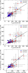 |
Fig. 6 Comparison between the kinetic temperatures derived from pyRADEX+MCMC modeling and using the p–H2CO integrated line intensities ratios R1 (top panel) and R2 (middle panel). Bottom panel: comparison of the kinetic temperatures derived from R1 and R2. The LTE temperature uncertainties are from uncertainties in the integrated intensities of the observed p–H2CO lines. The dashed black lines indicate a slope of unity. |
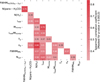 |
Fig. 7 Correlation matrix showing the relationships between various physical properties of molecular gas, ionized gas, and dust clumps. The color bar and annotations indicate the Spearman’s correlation coefficients. We flagged and excluded correlations with p-values > 0.0013 (3σ), thereby removing statistically insignificant relationships. |
5.2 Benchmarking the H2CO thermometer in H II regions
5.2.1 Comparing gas kinetic temperature and line width
The values of Tkin, derived using the non-LTE radiative transfer analysis presented in Sect. 4.2 are found to be consistently warmer than those derived from the dust emission. Additionally, 17 sources display blue- or red-skewed p–H2CO line profiles, indicating the presence of outflow or infall motions and associated shocked gas. The observed line profiles and derived gas temperatures of H2CO suggest that its formation is likely driven by shock heating or outflows and is located close to the H II regions within the parent molecular cloud (Ginsburg et al. 2011; Tang et al. 2017, 2018b).
In Fig. 8, we compare the gas kinetic temperature and line width obtained from the different gas tracers toward the H II regions by Giannetti et al. (2017). This shows that p–H2CO traces a wide range of the gas temperature and the traced temperature is hotter than molecules such as NH3. This is based on the findings of Wienen et al. (2012), who reported NH3 rotational temperatures in the range of 10–28 K and kinetic temperatures between 12 and 35 K. However, these authors note that the low-Eu (NH3 (1,1) and (2,2)) transitions used in their analysis exhibited different line widths, indicating that the observed NH3 transitions likely do not trace the same gas. Consequently, assuming equal beam-filling factors for these transitions represents only an approximation and may affect the radiative analysis and the subsequently derived NH3-bearing gas temperatures. This conclusion is further supported by Giannetti et al. (2017), who showed that these low-lying transitions of NH3 are not an optimal tracers of warm gas. Similarly, p–H2CO traces hotter regions compared to that traced by CH3CCH. Giannetti et al. (2017) found two temperature components associated with the CH3OH and CH3CN namely, hot and cool components with an average of 21 and 184 K, and 53 and 238 K for H II regions in their sample. The kinetic temperature derived using p–H2CO lies between the cool and hot component of CH3OH and CH3CN (see Fig. 8). Figure 8 (bottom) shows cumulative distribution function (CDF) comparisons of the molecular line width of different gas tracers. Although the Anderson-Darling test reveals that the distribution of line width of p–H2CO and CH3CCH, CH3OH (cool component) shows no significant differences, that of the warm components show significant differences. The mean value of the line widths of p–H2CO is greater than CH3CCH and NH3 and is less than CH3OH (hot component) and CH3CN (hot component). In contrast, the line width of p–H2CO is similar to the line width of CH3OH (hot component) and CH3CN (hot component). If the observed line widths of different molecular tracers were determined purely by thermal motion, they would depend directly on the gas temperature and inversely on the molecular mass. In reality, however, these line widths include both thermal and nonthermal contributions, making direct comparisons between tracers more complex.
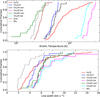 |
Fig. 8 Cumulative distribution functions for temperatures (top panel) and line width (bottom panel) for different H II regions. Different colors represent various tracers and components, as indicated in the legend. The NH3 properties are from Wienen et al. (2012). The CH3CCH, CH3OH (hot and cold), and CH3CN (hot and cold) properties are from Giannetti et al. (2017), whereas dust properties are from Urquhart et al. (2018). |
5.2.2 Chemical modeling
In this section, we aim to compare the position of H2CO relative to the different photodissociation region (PDR) tracers and dense gas tracers around H II regions. We used an updated version (v7.0) of the Meudon PDR code (Le Petit et al. 2006)11 to compare our observations with PDR models and investigate the chemical complexity surrounding an H II region for a typical density-temperature structure. Using the Meudon code, we ran models of constant thermal pressure (isobaric) across a 1D PDR in slab geometry, with a fixed pressure of 4.6×10⁷ K cm−3, determined by the average n(H2) and Tkin as traced by H2CO toward our sample (see Sects. 4.1 and 4.2). Combining the given density and temperature profiles with external sources of energy: the UV radiation field (G0) and cosmic-ray ionization rate (ζ), the code determines the abundance of each species by solving the chemical reactions under steady-state conditions. In addition to the external radiation fields described above, we included an internal stellar component—representing irradiation from host star(s)—and an isotropic ambient component. The isotropic field incorporates the interstellar radiation field with a value of 0.5 (in Habing units) on both the observer-facing and the backside of the cloud, as well as blackbody components that simulate dust infrared emission and the cosmic microwave background. A minimal external field is used such that illumination on the backside of the PDR is dominated by the stellar component. This isolates the cloud from external influences, focusing only on the effect of the embedded H II region on the surrounding molecular material.
We estimated the far-UV flux, G0, assuming that a single massive star is responsible for generating the H II region, from the massive stars that dominate the ionizing photon production in the sources studied. In Paper I, we derived the Lyman continuum photon flux for our sample using integrated radio flux measurements, finding a median value of 1.18 × 1048 s−1. This flux corresponds to a stellar spectral type of O5.5V–O5V with an effective surface temperature of approximately 41000 K (Martins et al. 2005). We assumed that the distance between the star and the PDR boundary (d0) is equal to the radius of H II region, which in our sample has a median value of 0.26 pc. This setup yields a stellar far-UV flux at the PDR surface of G0 ~ 5.3 × 10⁴ in units of the Habing field (1.6 × 10⁻³ erg cm−2 s−1; Habing 1968). We note that this estimate of G0 likely represents a lower limit, as the Lyman continuum flux derived from interferometric radio observations may underestimate the total radio flux, thus leading to an underestimation of the ionizing photon rate. In addition, absorption of UV photons by surrounding dust can further reduce the inferred value. Additionally, the relatively low spatial resolution (25″) of the RRL data used in Paper I could have led to an overestimated H II region size. To explore this further, we also ran the PDR models using a smaller star–PDR distance of d0 = 0.12 pc, which is the 16th percentile of our sample H II region size, this results in G0 values of ~2.5 × 10⁵ in units of Habing field. Both sets of models were run for a fixed value of cosmic-ray ionization rate of H2 molecules, ζ = 5 × 10⁻¹⁷ s−1, that lies between estimations in diffuse and dense gas (Indriolo et al. 2015; Le Petit et al. 2004). We assumed a total visual extinction of Amax = 10 mag for the cloud and adopted the extinction curve of HD 38087 (Fitzpatrick & Massa 1990) with RV = 5.6. For the modeling, we used an intermediate value for the column density to reddening ratio, NH/E(B − V) = 1.05 × 1022 cm−2 mag−1 (Joblin et al. 2018) and a dust-to-gas mass ratio of 0.01.
A schematic representation of the modeled profile across the H II region associated PDR is presented in Fig. 9 while the results of the Meudon PDR code simulations for d0 = 0.26 pc (left panel) and d0 = 0.12 pc (right panel) are presented in Fig. A.5. The central and bottom panels plot normalized molecular line abundances, n(x)/npeak(x), against AV for PDR tracers (c − C3H2, C2H, CO+, C+; Rizzo et al. 2005; Kim et al. 2020) and dense, molecular gas tracers (CN, CH3OH, C18O, H2CO; Kim et al. 2020), respectively, alongside the corresponding gas density (nH+, nH and nH2) and Tkin profiles. Consistently between the two sets of models, the PDR tracers peak at low values of n(H2) ~ 8 × 10³ to 5.6 × 105 cm−3 (AV = 2–5 mag, yellow shaded region in Fig. A.5) and Tkin ~ 900–70 K probing the dissociation front and translucent gas layers. However, as Av and n(H2) increase, the abundances of dense gas tracers such as C18O increase, peaking at AV ~ 8 mag.
Notably, we observed both H2CO and CH3OH exhibit enhanced abundances near the PDR interface, where the gas temperature reaches a few hundred kelvin and the density is around 104–5 cm−3. This abundance, intermediate to that seen by typical PDR and dense gas tracers, is expected and provides insight into the chemistry of these two species. For instance, CH3OH, the simplest complex organic molecule (COM; Herbst & van Dishoeck 2009) is formed efficiently in cold environments on grain surfaces by the continuous hydrogenation of CO (Fuchs et al. 2009) and by H-abstraction reactions of icy radicals (Álvarez-Barcia et al. 2018; Simons et al. 2020; Santos et al. 2022). CH3OH is subsequently released into the gas phase via thermal sublimation or nonthermal desorption processes where the presence of elevated temperatures in the form of shocks, aids this release via sputtering. This explains the CH3OH abundance peak seen at moderate AV ’s and high temperatures, highlighting that the formation of CH3OH only proceeds efficiently on grain surfaces and not in the gas phase. On the other hand, although H2CO is an important precursor for the formation of CH3OH on grains, unlike CH3OH, H2CO can also form in the cold gas-phase through neutral-neutral reactions between CH2 and O2 or CH3and O (Ramal-Olmedo et al. 2021) or ion-neutral reactions between ![Mathematical equation: $\[\mathrm{CH}_{3}^{+}\]$](/articles/aa/full_html/2026/02/aa58059-25/aa58059-25-eq6.png) and OH (Woodall et al. 2007). This reinforces the role of H2CO as an excellent tracer of gas kinetic temperature (Mangum & Wootten 1993). In addition with increasing UV-radiation field the PDR model produces higher abundances of H2CO consistent with observation result toward massive star forming regions (Immer et al. 2014; Tang et al. 2018b).
and OH (Woodall et al. 2007). This reinforces the role of H2CO as an excellent tracer of gas kinetic temperature (Mangum & Wootten 1993). In addition with increasing UV-radiation field the PDR model produces higher abundances of H2CO consistent with observation result toward massive star forming regions (Immer et al. 2014; Tang et al. 2018b).
Our Meudon PDR models (Fig. A.5) reproduce H2CO at gas densities consistent with our non-LTE PyRADEX results but at Tkin values of a few times 100 K. While a subset of p–H2CO velocity components shows high temperature (Fig. 3) the PDR models fail to reproduce significant amount of cooler H2CO. This could be because we carried out single-pointing observations which represent averaged spectra toward each clump, the multicomponent profiles likely arise from multiple molecular clumps within the beam, each with distinct velocities and physical conditions. Additional sources of uncertainty include the source specific n(H2)–Tkin profile assumed. Moreover, the broader, higher-temperature components probably trace gas affected by outflows, inflows, or shocks. In the following section, we examine the origin and nature of these “H2CO Sub” components in detail.
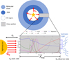 |
Fig. 9 Schematic depicting a fully evolved H II region in which accretion onto the central star has ceased but the region remains embedded in its surrounding environment. Additionally, it outlines the various input parameters used in the Meudon PDR code and output molecular abundance as presented in Fig. A.5. |
5.3 Nature of secondary component (H2CO Sub)
The p–H2CO observations reveal multiple velocity components in a large fraction of the sources in our sample. We classify these components as “H2CO Main” and “H2CO Sub” based on their centroid velocities, as described in Sect. 3.1. In this section, we investigate the nature and origin of the “H2CO Sub” components. As discussed in Sect. 5.2, H2CO forms in regions with layered density and temperature structures, which can produce multiple velocity components in the observed line profiles. The Meudon PDR models reproduce strong H2CO emission from high-UV PDR (Fig. A.5). Because these layers lie near the surface of H II regions, they are subject to intense UV radiation, gas inflow/outflow, and turbulent motions, which broaden the observed lines.
Figure 10a shows the distribution of the p–H2CO (30,3–20,2) FWHM, indicating that the H2CO Sub components exhibit systematically broader lines than the Main components, consistent with turbulence-driven broadening. Using the Tkin derived in Sect. 4.2, we calculated the thermal and nonthermal velocity dispersions for each component as
![Mathematical equation: $\[\sigma_{\mathrm{T}}=\sqrt{\frac{k T_{\mathrm{kin}}}{m_{\mathrm{H}_2 \mathrm{CO}}}}, \quad \sigma_{\mathrm{NT}}=\sqrt{\left(\frac{\Delta v}{8 ~\ln~ 2}\right)^2-\sigma_{\mathrm{T}}^2},\]$](/articles/aa/full_html/2026/02/aa58059-25/aa58059-25-eq7.png) (4)
(4)
where k is the Boltzmann constant, Δv is the p–H2CO (30,3–20,2) FWHM, and mH2CO is the mass of a formaldehyde molecule. The thermal line width is significantly lower than the nonthermal line width for H2CO with a median of 0.13 and 0.8 km s−1, respectively, indicating that nonthermal processes dominate the line broadening. This result is consistent with Tang et al. (2018b). Figure 10b further shows that the H2CO Sub components have higher nonthermal line widths (median ~0.92 km s−1) than the Main components (median ~0.70 km s−1). This enhancement is likely due to the fact the H2CO Sub components arise from turbulence and shock motions near the surfaces of H II regions.
The median sound speed (![Mathematical equation: $\[a_{\mathrm{s}}=\sqrt{\frac{k T_{\mathrm{kin}}}{\mu m_{\mathrm{H}}}}\]$](/articles/aa/full_html/2026/02/aa58059-25/aa58059-25-eq8.png) , where μ = 2.7 is the mean molecular weight for molecular clouds and mH is the mass of the hydrogen atom) is ~0.45 km s−1 at a temperature of 66 K. This gives the median Mach number (given as M = σNT/as) of 2.45 and 1.56 for the Sub and Main components, respectively, confirming that the H2CO Sub components are dominated by supersonic nonthermal motions and trace strongly turbulent gas within our sample.
, where μ = 2.7 is the mean molecular weight for molecular clouds and mH is the mass of the hydrogen atom) is ~0.45 km s−1 at a temperature of 66 K. This gives the median Mach number (given as M = σNT/as) of 2.45 and 1.56 for the Sub and Main components, respectively, confirming that the H2CO Sub components are dominated by supersonic nonthermal motions and trace strongly turbulent gas within our sample.
We examined the relationship between the nonthermal line width of p–H2CO and the clump bolometric luminosity for the H2CO transitions. Figure 10c presents this correlation, where the nonthermal line width serves as a proxy for turbulent motion. We fit a power-law relation for three cases: all components combined, H2CO Main components, and H2CO Sub components, with the fitting results summarized in Table 2. The nonthermal line width shows a positive correlation with Lbol, indicating that turbulence in molecular clouds increases with luminosity. This trend suggests that more luminous sources are associated with more turbulent molecular environments (Wang et al. 2009).
The relationship between σNT of p–H2CO (30,3–20,2) and Lbol follows a power law of the form ![Mathematical equation: $\[\sigma_{\mathrm{NT}} \propto L_{\text {bol}}^{0.1-0.16}\]$](/articles/aa/full_html/2026/02/aa58059-25/aa58059-25-eq9.png) (see Table 2). The slope is steeper for the H2CO Sub component (0.16) than for the H2CO Main component (0.10), supporting the interpretation that the H2CO Sub emission originates from regions more influenced by massive stars, where turbulence is enhanced—likely near the ionization fronts of H II regions.
(see Table 2). The slope is steeper for the H2CO Sub component (0.16) than for the H2CO Main component (0.10), supporting the interpretation that the H2CO Sub emission originates from regions more influenced by massive stars, where turbulence is enhanced—likely near the ionization fronts of H II regions.
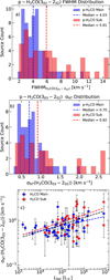 |
Fig. 10 Distributions of (a) FWHM and (b) σNT of the p–H2CO (30,3–20,2) transition. The blue and red histograms represent the H2CO Main and H2CO Sub components, respectively, with the corresponding dashed lines marking their median values. Panel c: relation between σNT and Lbol. The black, blue, and red dashed lines indicate the power-law fits for all components combined, the Main components, and the Sub components, respectively. |
Clump bolometric luminosity versus σNT (p–H2CO (30,3–20,2)) nonthermal line width.
5.4 Molecular pressure and confinement of H II region
H II region expand under the ionized gas pressure but are impeded by the ambient molecular gas pressure. Figure 11 (left) compares the thermal pressures of the ionized and molecular gas components. For nearly all sources in our sample, the molecular gas pressure exceeds that of the ionized gas. This implies that the molecular gas pressure can slow down the expansion of embedded H II regions. Moreover showing that high molecular gas pressure persists regardless of the velocity offset between RRLs and p–H2CO transitions, further supporting the argument that molecular pressure can confine the expansion of embedded H II regions.
However, several caveats exist. Firstly, these H II regions must still be embedded within their natal molecular clumps; our observations though limited by spectral resolution, try to fulfill this condition through our selection of H II regions with sizes smaller than their parental ATLASGAL clump (Sect. 2.1). Secondly, the molecular pressures derived from H2CO should trace gas closer to the ionization front, this is supported by both observations and the Meudon PDR models (Sect. 5.2). A confirmation of the same awaits higher resolution H2CO and ionized gas mapping. Thirdly, the ionized gas parameters (ne, Te) adopted from Paper I represent spatial averages that may underestimate the true pressure at the ionization boundary. Figure 11 (right) compares the ionized gas pressures with those derived from dust emission at 870 μm (Urquhart et al. 2018, 2022), representing the average clump conditions. In this case, the ionized gas pressure often exceeds that of the molecular component. In contrast to the molecular gas, the pressures inferred from dust emission may not be representative of conditions in the vicinity of the expanding H II regions. Resolving these apparent inconsistencies will require high-resolution observations of the ionized and molecular gas interfaces.
Recently, Faerber et al. (2025) analyzed the expansion signatures of 35 H II regions mapped in [CII] 158 μm emission. Among these, 12 H II regions were identified as candidates for expansion, and eight of them were consistent with a spherical expansion model. They also found that thermal pressure and stellar winds are the primary drivers of H II region expansion in their sample. Previous studies, including that of Anderson et al. (2011) and Paper I, reported that roughly 50% of cataloged Galactic H II regions exhibit bubble-like morphologies at 8 μm, based on GLIMPSE images (Benjamin et al. 2003), which trace PDRs. In our sample, 23 sources exhibit bubble morphology including irregular bubbles and of the remaining 19 sources show compact morphology. To explore these processes in more detail, maps of PDRs and dense molecular gas tracers in the vicinity of expanding H II regions are needed, along with radio continuum and RRL observations at optically thin frequencies. Such observations will allow a detailed analysis of both ionized and molecular gas, as well as high-resolution studies of the gas dynamics. This approach will provide stronger constraints on the formation, evolution, and feedback mechanisms of H II regions.
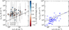 |
Fig. 11 Comparison between the thermal pressure of ionized and molecular gas. The color bar indicates the velocity difference between the RRL and p–H2CO transitions. Left panel: n(H2) and Tkin derived from p–H2CO in this work. Right panel: n(H2) and Tdust estimated from the 870 μm emission (Urquhart et al. 2018, 2022), representing the average clump pressure. The dashed black lines mark the slope of equal pressure. The plots are set to the same scale for visual comparison. |
6 Conclusion and summary
We have investigated the physical properties traced by molecular and ionized gas in a statistically significant sample of H II regions associated with ATLASGAL dust clumps. We used observations carried out with the APEX 12 m submillimeter telescope of multiple transitions of p–H2CO associated with its J=3–2 and 4–3 transitions toward these sources. In our earlier study (Paper I), we examined the ionized gas properties of H II regions using centimeter–RRLs from the GLOSTAR survey. In this work, we focused on the molecular gas properties of the embedded H II regions and compared them with the ionized gas characteristics. Our main findings are summarized below:
We constrained the physical properties of massive clumps associated with H II regions by deriving the gas density and kinetic temperature for 52 clumps. We carried out non-LTE radiative transfer modeling of the six p–H2CO transitions studied, which serve as effective tracers of density and temperature in dense gas, using PyRADEX+MCMC. The resulting Tkin ranges from 33.7 K to 265 K, with a median value of ~66 K and n(H2) > 105 cm−3 across our sample, and it aligns with findings from previous studies;
We analyzed the relationships among the physical properties of dust, molecular gas, and ionized gas by calculating the Spearman correlation coefficients and p-values for various parameters. Properties that directly depend on the central high-mass star, such as Lbol and NLyc, exhibit stronger and more frequent correlations with other parameters. This suggests that the central high-mass star largely governs and influences the physical conditions of the surrounding dust, ionized gas, and molecular gas;
By comparing H2CO with other molecular gas tracers, we found that H2CO traces denser gas located near the interface between the H II region and the surrounding molecular cloud. The Meudon PDR models reproduced H2CO abundances peaking near the ionized region’s surface and at gas densities similar to those obtained from PyRADEX but at high values of Tkin. Understanding the origins of the cooler H2CO components requires further investigation with more detailed modelling;
The nature of the “H2CO Sub” components reveals that these components are dominated by supersonic nonthermal motions and trace turbulent gas;
We investigated whether the surrounding molecular gas confines the expansion of H II regions through excess pressure. Our analysis shows that for most of our sources, the pressure of the neutral gas exceeds that of the ionized gas, regardless of the velocity difference between the ionized and molecular components. This finding suggests that the surrounding neutral molecular gas can slow down or hinder the expansion of H II regions due to its higher pressure. However, there are several caveats, and a confirmation of this fining relies on future high resolution mapping of H II regions and their surroundings in RRL and molecular lines. Such observations will soon be achievable with the unprecedented sensitivity and spatial resolution offered by next-generation radio facilities such as the ngVLA and SKA–Mid.
The expansion and feedback of H II regions significantly shape the ISM, regulate star formation rates, and influence galactic evolution. Future studies should increase the sample size of embedded and expanding H II regions to better explore the relationship between ionized and molecular gas. This will improve our understanding of how H II regions evolve over time and impact their surrounding molecular environment. Placing tighter constraints on the connection between ionized and molecular gas across various evolutionary stages ranging from compact to classical diffuse H II regions will be essential for understanding their development and potential role in triggering star formation.
Data availability
Tables C.1, C.2, and C.3 are available at the CDS via https://cdsarc.cds.unistra.fr/viz-bin/cat/J/A+A/706/A280
Acknowledgements
During the preparation of this article, we suffered the tragic loss of Prof. Dr Karl M. Menten, S.K.’s PhD supervisor and the principal investigator of the GLOSTAR survey. We dedicate this work to his enduring legacy. We are deeply indebted to the countless discussions with him that have inspired generations of radio astronomers. We will always miss his warmth, wisdom, boundless curiosity, generosity of spirit, kindness, and delightful sense of humor. We sincerely thank the referee for their positive, timely, and constructive feedback. We thank MPIfR and APEX staff for operating the observatory and collecting the data (https://www.apex-telescope.org/ns/). This research made use of information from the ATLASGAL database at (http://atlasgal.mpifr-bonn.mpg.de/cgi-bin/ATLASGAL_DATABASE.cgi) supported by the MPIfR, Bonn. A.M.J. acknowledges support by the CRC1601 (SFB 1601 subproject B2) funded by the DFG (German Research Foundation) – 500700252. S.K. and A.M.J. thanks the Max Planck Society for their support. Y.G. was supported by the Ministry of Science and Technology of China under the National Key R&D Program under grant No. 2023YFA1608200, the National Natural Science Foundation of China (NSFC) under grant No. 12427901, and the Strategic Priority Research Program of the Chinese Academy of Sciences under grant No. XDB0800301. S.N. gratefully acknowledges the Collaborative Research Center 1601 (SFB 1601 subproject B1) funded by the Deutsche Forschungsgemeinschaft (DFG, German Research Foundation) – 500700252. This research has made use of the SIMBAD database and the VizieR catalog, operated at CDS, Strasbourg, France. This research made use of Astropy (http://www.astropy.org), a community developed core Python package for Astronomy (Astropy Collaboration 2022). This document was prepared using the collaborative tool Overleaf available at: https://www.overleaf.com/.
References
- Altenhoff, W. J., Downes, D., Pauls, T., & Schraml, J. 1979, A&AS, 35, 23 [Google Scholar]
- Álvarez-Barcia, S., Russ, P., Kästner, J., & Lamberts, T. 2018, MNRAS, 479, 2007 [Google Scholar]
- Anderson, L. D., Bania, T. M., Balser, D. S., & Rood, R. T. 2011, ApJS, 194, 32 [NASA ADS] [CrossRef] [Google Scholar]
- Anderson, L. D., Bania, T. M., Balser, D. S., et al. 2014, ApJS, 212, 1 [Google Scholar]
- Ao, Y., Henkel, C., Menten, K. M., et al. 2013, A&A, 550, A135 [NASA ADS] [CrossRef] [EDP Sciences] [Google Scholar]
- Astropy Collaboration (Price-Whelan, A. M., et al.) 2022, ApJ, 935, 167 [NASA ADS] [CrossRef] [Google Scholar]
- Benjamin, R. A., Churchwell, E., Babler, B. L., et al. 2003, PASP, 115, 953 [Google Scholar]
- Brunthaler, A., Menten, K. M., Dzib, S. A., et al. 2021, A&A, 651, A85 [EDP Sciences] [Google Scholar]
- Csengeri, T., Urquhart, J. S., Schuller, F., et al. 2014, A&A, 565, A75 [NASA ADS] [CrossRef] [EDP Sciences] [Google Scholar]
- Deharveng, L., Zavagno, A., Salas, L., et al. 2003, A&A, 399, 1135 [NASA ADS] [CrossRef] [EDP Sciences] [Google Scholar]
- Deharveng, L., Schuller, F., Anderson, L. D., et al. 2010, A&A, 523, A6 [NASA ADS] [CrossRef] [EDP Sciences] [Google Scholar]
- Downes, D., Wilson, T. L., Bieging, J., & Wink, J. 1980, A&AS, 40, 379 [Google Scholar]
- Du, Z. M., Zhou, J. J., Esimbek, J., Han, X. H., & Zhang, C. P. 2011, A&A, 532, A127 [NASA ADS] [CrossRef] [EDP Sciences] [Google Scholar]
- Dzib, S. A., Yang, A. Y., Urquhart, J. S., et al. 2023, A&A, 670, A9 [NASA ADS] [CrossRef] [EDP Sciences] [Google Scholar]
- Elmegreen, B. G. 2011, in EAS Publications Series, 51, eds. C. Charbonnel, & T. Montmerle (EDP), 45 [Google Scholar]
- Elmegreen, B. G., & Lada, C. J. 1977, ApJ, 214, 725 [Google Scholar]
- Endres, C. P., Schlemmer, S., Schilke, P., Stutzki, J., & Müller, H. S. P. 2016, J. Mol. Spectrosc., 327, 95 [NASA ADS] [CrossRef] [Google Scholar]
- Fabricant, B., Krieger, D., & Muenter, J. S. 1977, J. Chem. Phys., 67, 1576 [NASA ADS] [CrossRef] [Google Scholar]
- Faerber, T., Anderson, L. D., Luisi, M., et al. 2025, arXiv e-prints [arXiv:2506.16700] [Google Scholar]
- Fitzpatrick, E. L., & Massa, D. 1990, ApJS, 72, 163 [NASA ADS] [CrossRef] [Google Scholar]
- Foreman-Mackey, D., Farr, W., Sinha, M., et al. 2019, J. Open Source Softw., 4, 1864 [NASA ADS] [CrossRef] [Google Scholar]
- Fuchs, G. W., Cuppen, H. M., Ioppolo, S., et al. 2009, A&A, 505, 629 [NASA ADS] [CrossRef] [EDP Sciences] [Google Scholar]
- Gao, X. Y., Reich, P., Hou, L. G., Reich, W., & Han, J. L. 2019, A&A, 623, A105 [NASA ADS] [CrossRef] [EDP Sciences] [Google Scholar]
- Gerner, T., Beuther, H., Semenov, D., et al. 2014, A&A, 563, A97 [NASA ADS] [CrossRef] [EDP Sciences] [Google Scholar]
- Giannetti, A., Leurini, S., Wyrowski, F., et al. 2017, A&A, 603, A33 [NASA ADS] [CrossRef] [EDP Sciences] [Google Scholar]
- Ginsburg, A., Darling, J., Battersby, C., Zeiger, B., & Bally, J. 2011, ApJ, 736, 149 [NASA ADS] [CrossRef] [Google Scholar]
- Gong, Y., Ortiz-León, G. N., Rugel, M. R., et al. 2023, A&A, 678, A130 [NASA ADS] [CrossRef] [EDP Sciences] [Google Scholar]
- Güsten, R., Nyman, L. Å., Schilke, P., et al. 2006, A&A, 454, L13 [NASA ADS] [CrossRef] [EDP Sciences] [Google Scholar]
- Habing, H. J. 1968, Bull. Astron. Inst. Netherlands, 19, 421 [Google Scholar]
- Henkel, C., Wilson, T. L., Walmsley, C. M., & Pauls, T. 1983, A&A, 127, 388 [NASA ADS] [Google Scholar]
- Herbst, E., & van Dishoeck, E. F. 2009, ARA&A, 47, 427 [Google Scholar]
- Immer, K., Galván-Madrid, R., König, C., Liu, H. B., & Menten, K. M. 2014, A&A, 572, A63 [NASA ADS] [CrossRef] [EDP Sciences] [Google Scholar]
- Indriolo, N., Neufeld, D. A., Gerin, M., et al. 2015, ApJ, 800, 40 [NASA ADS] [CrossRef] [Google Scholar]
- Joblin, C., Bron, E., Pinto, C., et al. 2018, A&A, 615, A129 [NASA ADS] [CrossRef] [EDP Sciences] [Google Scholar]
- Kalcheva, I. E., Hoare, M. G., Urquhart, J. S., et al. 2018, A&A, 615, A103 [NASA ADS] [CrossRef] [EDP Sciences] [Google Scholar]
- Khan, S., Rugel, M. R., Brunthaler, A., et al. 2024, A&A, 689, A81 [NASA ADS] [CrossRef] [EDP Sciences] [Google Scholar]
- Kim, W. J., Wyrowski, F., Urquhart, J. S., et al. 2020, A&A, 644, A160 [NASA ADS] [CrossRef] [EDP Sciences] [Google Scholar]
- Klein, B., Hochgürtel, S., Krämer, I., et al. 2012, A&A, 542, L3 [NASA ADS] [CrossRef] [EDP Sciences] [Google Scholar]
- Kuchar, T. A., & Clark, F. O. 1997, ApJ, 488, 224 [NASA ADS] [CrossRef] [Google Scholar]
- Kurtz, S. 2005, in IAU Symposium, 227, Massive Star Birth: A Crossroads of Astrophysics, eds. R. Cesaroni, M. Felli, E. Churchwell, & M. Walmsley, 111 [Google Scholar]
- Le Petit, F., Roueff, E., & Herbst, E. 2004, A&A, 417, 993 [NASA ADS] [CrossRef] [EDP Sciences] [Google Scholar]
- Le Petit, F., Nehmé, C., Le Bourlot, J., & Roueff, E. 2006, ApJS, 164, 506 [NASA ADS] [CrossRef] [Google Scholar]
- Lockman, F. J. 1989, ApJS, 71, 469 [Google Scholar]
- Mangum, J. G., & Wootten, A. 1993, ApJS, 89, 123 [Google Scholar]
- Mangum, J. G., Wootten, A., Loren, R. B., & Wadiak, E. J. 1990, ApJ, 348, 542 [NASA ADS] [CrossRef] [Google Scholar]
- Mangum, J. G., Darling, J., Henkel, C., & Menten, K. M. 2013, ApJ, 766, 108 [NASA ADS] [CrossRef] [Google Scholar]
- Martins, F., Schaerer, D., & Hillier, D. J. 2005, A&A, 436, 1049 [NASA ADS] [CrossRef] [EDP Sciences] [Google Scholar]
- McCauley, P. I., Mangum, J. G., & Wootten, A. 2011, ApJ, 742, 58 [Google Scholar]
- Medina, S. N. X., Urquhart, J. S., Dzib, S. A., et al. 2019, A&A, 627, A175 [NASA ADS] [CrossRef] [EDP Sciences] [Google Scholar]
- Medina, S. N. X., Dzib, S. A., Urquhart, J. S., et al. 2024, A&A, 689, A196 [NASA ADS] [CrossRef] [EDP Sciences] [Google Scholar]
- Meledin, D., Lapkin, I., Fredrixon, M., et al. 2022, A&A, 668, A2 [NASA ADS] [CrossRef] [EDP Sciences] [Google Scholar]
- Molinari, S., Pezzuto, S., Cesaroni, R., et al. 2008, A&A, 481, 345 [NASA ADS] [CrossRef] [EDP Sciences] [Google Scholar]
- Molinari, S., Merello, M., Elia, D., et al. 2016, ApJ, 826, L8 [Google Scholar]
- Motte, F., Bontemps, S., & Louvet, F. 2018, ARA&A, 56, 41 [Google Scholar]
- Müller, H. S. P., Thorwirth, S., Roth, D. A., & Winnewisser, G. 2001, A&A, 370, L49 [Google Scholar]
- Müller, H. S. P., Schlöder, F., Stutzki, J., & Winnewisser, G. 2005, J. Mol. Struct., 742, 215 [Google Scholar]
- Ossenkopf, V., & Henning, T. 1994, A&A, 291, 943 [NASA ADS] [Google Scholar]
- Ramal-Olmedo, J. C., Menor-Salván, C. A., & Fortenberry, R. C. 2021, A&A, 656, A148 [NASA ADS] [CrossRef] [EDP Sciences] [Google Scholar]
- Reid, M. J., Menten, K. M., Brunthaler, A., et al. 2019, ApJ, 885, 131 [Google Scholar]
- Reifenstein, E. C., Wilson, T. L., Burke, B. F., Mezger, P. G., & Altenhoff, W. J. 1970, A&A, 4, 357 [NASA ADS] [Google Scholar]
- Rizzo, J. R., Fuente, A., & García-Burillo, S. 2005, ApJ, 634, 1133 [NASA ADS] [CrossRef] [Google Scholar]
- Santos, J. C., Chuang, K.-J., Lamberts, T., et al. 2022, ApJ, 931, L33 [NASA ADS] [CrossRef] [Google Scholar]
- Schuller, F., Menten, K. M., Contreras, Y., et al. 2009, A&A, 504, 415 [NASA ADS] [CrossRef] [EDP Sciences] [Google Scholar]
- Sewilo, M., Churchwell, E., Kurtz, S., Goss, W. M., & Hofner, P. 2004, ApJ, 605, 285 [Google Scholar]
- Simons, M. A. J., Lamberts, T., & Cuppen, H. M. 2020, A&A, 634, A52 [NASA ADS] [CrossRef] [EDP Sciences] [Google Scholar]
- Tang, X. D., Henkel, C., Menten, K. M., et al. 2017, A&A, 598, A30 [NASA ADS] [CrossRef] [EDP Sciences] [Google Scholar]
- Tang, X. D., Henkel, C., Menten, K. M., et al. 2018a, A&A, 609, A16 [NASA ADS] [CrossRef] [EDP Sciences] [Google Scholar]
- Tang, X. D., Henkel, C., Wyrowski, F., et al. 2018b, A&A, 611, A6 [NASA ADS] [CrossRef] [EDP Sciences] [Google Scholar]
- Tang, X. D., Henkel, C., Menten, K. M., et al. 2021, A&A, 655, A12 [NASA ADS] [CrossRef] [EDP Sciences] [Google Scholar]
- Thompson, M. A., Urquhart, J. S., Moore, T. J. T., & Morgan, L. K. 2012, MNRAS, 421, 408 [NASA ADS] [Google Scholar]
- Urquhart, J. S., Busfield, A. L., Hoare, M. G., et al. 2007, A&A, 461, 11 [NASA ADS] [CrossRef] [EDP Sciences] [Google Scholar]
- Urquhart, J. S., Hoare, M. G., Purcell, C. R., et al. 2009, A&A, 501, 539 [NASA ADS] [CrossRef] [EDP Sciences] [Google Scholar]
- Urquhart, J. S., Thompson, M. A., Moore, T. J. T., et al. 2013, MNRAS, 435, 400 [Google Scholar]
- Urquhart, J. S., König, C., Giannetti, A., et al. 2018, MNRAS, 473, 1059 [Google Scholar]
- Urquhart, J. S., Wells, M. R. A., Pillai, T., et al. 2022, MNRAS, 510, 3389 [NASA ADS] [CrossRef] [Google Scholar]
- van der Tak, F. F. S., Black, J. H., Schöier, F. L., Jansen, D. J., & van Dishoeck, E. F. 2007, A&A, 468, 627 [NASA ADS] [CrossRef] [EDP Sciences] [Google Scholar]
- Wang, K., Wu, Y. F., Ran, L., Yu, W. T., & Miller, M. 2009, A&A, 507, 369 [NASA ADS] [CrossRef] [EDP Sciences] [Google Scholar]
- Wienen, M., Wyrowski, F., Schuller, F., et al. 2012, A&A, 544, A146 [NASA ADS] [CrossRef] [EDP Sciences] [Google Scholar]
- Wiesenfeld, L., & Faure, A. 2013, MNRAS, 432, 2573 [NASA ADS] [CrossRef] [Google Scholar]
- Woodall, J., Agúndez, M., Markwick-Kemper, A. J., & Millar, T. J. 2007, A&A, 466, 1197 [CrossRef] [EDP Sciences] [Google Scholar]
- Yang, C., Omont, A., Beelen, A., et al. 2017, A&A, 608, A144 [NASA ADS] [CrossRef] [EDP Sciences] [Google Scholar]
- Yang, A. Y., Dzib, S. A., Urquhart, J. S., et al. 2023, A&A, 680, A92 [NASA ADS] [CrossRef] [EDP Sciences] [Google Scholar]
This publication is based on data acquired with the APEX telescope (https://www.apex-telescope.org/ns). APEX telescope is operated and maintained by the Max-Planck-Institut für Radioastronomie, Bonn, Germany.
We report median values toward our sample throughout the paper, as the mean would be misleading given results at extremities that skew the distributions. This is most clearly seen in the distributions of the RADEX derived Tkin values as displayed in Fig. 4b.
For the components of AGAL031.412+00.307, the PyRADEX+MCMC did not converge to gas temperatures within the explored temperature range, resulting in lower limits set by the maximum gas temperature at which the collisional rate coefficients are computed.
Appendix A Additional figures
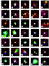 |
Fig. A.1 Three-color composite images of the targets of this study. The images combine mid–infrared data from Herschel 70 μm (red), MIPSGAL 24 μm (green), and GLIMPSE 8.0 μm (blue), overlaid with the GLOSTAR 5 GHz radio continuum contours in white. The filled white circle in corner represents the 25" beam of the radio continuum data from Paper I. Continued. |
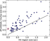 |
Fig. A.2 Comparison of physical size of H II regions and associated ATLASGAL clump size taken from Csengeri et al. (2014). The dashed black line shows the line of equality. The red circle represents only unresolved H II region, G030.720–0.082, in our sample. |
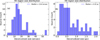 |
Fig. A.3 Distribution of (a) angular and (b) physical deconvolved FHWM size of H II region. The vertical dashed line shows the median value of the distribution. |
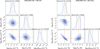 |
Fig. A.4 Example corner plot for AGAL045.121+00.131. To constrain physical properties of the molecular clouds we used the non-LTE RADEX modelling with MCMC algorithm, here we show the corresponding corner plot for each Gaussian component displaying the 1D histogram of the posterior distribution for each parameter (kinetic temperature, Tkin, H2 density, n(H2), and p–H2CO column density, N(p–H2CO)). The histograms represent the PDFs of the Monte Carlo fit parameters, while the blue curves represent the scatter plot of the joint distribution between the two parameters. The orange solid lines indicate the median of the PDFs, representing the most likely fit parameters, and the dotted blue lines correspond to the 1σ confidence intervals. The subtitle of each corner plot shows most likely value of the parameters with upper and lower 1σ error. |
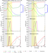 |
Fig. A.5 Meudon PDR model results for a constant thermal pressure of Pth ~ 4.6 × 10⁷ K cm−3. Left panel: Meudon PDR model run with input spectral type of O5V, distance to PDR of d0 = 0.26 pc, and far-UV flux, G0 ~ 5.3 × 10⁴ in units of Habing field. Right panel: Meudon PDR model run with input spectral type of O 5 V, distance to PDR of d0 = 0.12 pc, and far-UV flux, G0 ~ 2.5 × 10⁵ in units of Habing field. The top plots shows the evolution of hydrogen species – H2, H, and H+, as well as the gas temperature as a function of visual extinction AV. The middle and bottom plots present the spatial density profiles of key PDR and dense gas tracer molecules (see main text), where each density has been normalized to its maximum value within the cloud. |
Appendix B Effect of distance on source selection
In Sect. 2.1, we outlined the criteria used to select the sources, and Fig. 1 illustrates their distance distribution. To compare the physical conditions of the ionized and dense molecular gas, we adopted ionized gas parameters from Paper I. Because these parameters vary with distance, we examined the distance dependence within our sample. Figure B.1 shows the trends of NLyc, ne, and Te as a function of distance. While ne exhibits only a weak dependence and Te remains largely independent of distance, NLyc increases systematically, reflecting its strong distance dependence. This spread in NLyc indicates that our sample encompasses H II regions powered by a wide range of spectral type of central OB star. Overall, the distance variation introduces no significant bias in the derived ionized gas properties but rather ensures a diverse and representative sample.
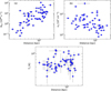 |
Fig. B.1 Relation between the distances and (a) NLyc, (b) ne, and (c) Te for our sample. |
Appendix C Tables
Line fitting parameters of the p–H2CO lines observed with nFLASH230.
Line fitting parameters of the p–H2CO lines observed with SEPIA345.
Derived physical properties of molecular clouds.
Appendix D Optical depth
Since much of the analysis presented above assumes optically thin conditions, we here examine the validity of this assumption. To assess the influence of optical depth on the derived quantities, we display in Fig. D.1 the PyRADEX+MCMC reproduced optical depths, τ, for the observed p–H2CO (30,3–20,2) transitions (which has the lowest value of Eu and the brightest observed transition) across the range of gas densities and p–H2CO column densities probed but for fixed values of Tkin, at median Tkin of 66 K (Fig. D.1 left) and at a higher Tkin of 200 K (Fig. D.1 right).
The background color scale represents the counts visualized over hexagonally binned distributions across the derived n(H2)–N(p–H2CO) space for our sample. The solid black curves mark contours of the optical depth equal to 1 and 5 at Tkin of 66 and 200 K. The blue dashed curves represent the beam filling factor corrected line intensities of the p–H2CO (30,3–20,2), corresponding to the brightest (TMB =8.26 K), median (TMB =0.94 K), and the lowest (TMB =0.18 K) detection in our sample. We find that all the observed p–H2CO transitions are optically thin (τ < 1) at column densities N(p–H2CO) < 1014 cm−2 and spatial densities n(H2) = 103–8 cm−3. We also notice that the transition becomes very optically thick (τ > 5), at column densities higher than 5 × 1015 cm−2. The spatial density and column density derived using the observed p–H2CO line intensities, shown as colored hexagonal bins in Fig. D.1, lie predominantly in or near the optically thin region (τ < 1). Among the observed p–H2CO transitions, the low-lying p–H2CO (30,3–20,2) line is the brightest, while the other transitions, which have higher, upper energy levels (Eu > 34 (K); see Table 1), are expected to have much lower optical depths (τ ≪ 1). This indicates that optical depth effects have only a minimal impact on the derived spatial densities and kinetic temperatures from the p–H2CO transitions. Furthermore, as was found by Tang et al. (2018b), varying the kinetic temperature only weakly affects the optical depth of the p–H2CO lines as evident from Fig. D.1.
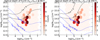 |
Fig. D.1 Optical depth of p–H2CO (30,3–20,2) as a function of n(H2)-N(p–H2CO) for a fix value of Tkin. The color hexagonally binned distributions display the PyRADEX+MCMC constrained n(H2) and N(p–H2CO) of our sources. The black solid curves show the optical depth of τ = 1 and 5 for p–H2CO (30,3–20,2) transition on top of n(H2) and N(p–H2CO) space, assuming fixed kinetic temperature of 66 K (the median temperature of our sample; left panel) and 200 K (higher temperature; right panel). The blue dashed curves indicate the contour corresponding to the brightest, average, and faintest observed intensities for p–H2CO (30,3–20,2) transition (see the text). |
All Tables
Clump bolometric luminosity versus σNT (p–H2CO (30,3–20,2)) nonthermal line width.
All Figures
|
Fig. 1 Galactic distribution of the source sample. The locations of the targets are denoted by red stars on an artistic rendering of the Milky Way. The distances to the observed H II regions and their associated clumps are taken from Paper I (and references therein). The spiral arms are marked following the description presented in Reid et al. (2019), and the individual spiral arms are colored as follows: the 3 kpc in magenta, the Norma-Outer Arm in red, the Scutum-Centaurus Arm in blue, the Sagittarius-Carina Arm in green, the Local Arm in cyan, and the Perseus Arm is in yellow. |
| In the text | |
|
Fig. 2 Spectra of the different p–H2CO and RRL transitions studied in this work toward AGAL045.121+00.131. Left panels: spectra of all six of the observed p–H2CO transitions (black) along with the multicomponent Gaussian fitting (green and magenta) and residual of the fitting (dashed blue). The total fit is displayed in red and the gray shaded region demarcates the 3σ level of the rms noise. The vertical dashed gray lines mark the centroid velocities of each fit Gaussian component. Right panel: spectra of the stacked GLOSTAR ⟨Hnα⟩ RRL in black alongside the Gaussian fit in red. Also displayed is the 5.3 GHz radio continuum emission map obtained with the GLOSTAR VLA D configuration toward this source and overlaid with white contours is the ATLASGAL 870 μm. The white filled circle shows the 25″ GLOSTAR beam. |
| In the text | |
|
Fig. 3 Distribution of the sources in the n(H2)–Tkin plane. The blue and red colors respectively represent sources with single and multiple component Gaussian profiles. Filled circles denote components classified as “H2CO Main,” while stars indicate those identified as “H2CO Sub.” |
| In the text | |
|
Fig. 4 Distributions of the pyRADEX+MCMC derived (a) n(H2), (b) Tkin, (c) N(p–H2CO), and (d) p–H2CO fractional abundance, X(p–H2CO) toward the different velocity components identified in our sample, as traced by the p–H2CO. The blue and red histograms represent the distributions for the “H2CO Main” and “H2CO Sub” components, respectively, while the corresponding dashed lines indicate the median values of each distribution. |
| In the text | |
|
Fig. 5 Comparison between n(H2) probed by 870 μm emission from dust and p–H2CO as derived from our pyRADEX+MCMC models. The dashed black line displays a slope of unit value. |
| In the text | |
|
Fig. 6 Comparison between the kinetic temperatures derived from pyRADEX+MCMC modeling and using the p–H2CO integrated line intensities ratios R1 (top panel) and R2 (middle panel). Bottom panel: comparison of the kinetic temperatures derived from R1 and R2. The LTE temperature uncertainties are from uncertainties in the integrated intensities of the observed p–H2CO lines. The dashed black lines indicate a slope of unity. |
| In the text | |
|
Fig. 7 Correlation matrix showing the relationships between various physical properties of molecular gas, ionized gas, and dust clumps. The color bar and annotations indicate the Spearman’s correlation coefficients. We flagged and excluded correlations with p-values > 0.0013 (3σ), thereby removing statistically insignificant relationships. |
| In the text | |
|
Fig. 8 Cumulative distribution functions for temperatures (top panel) and line width (bottom panel) for different H II regions. Different colors represent various tracers and components, as indicated in the legend. The NH3 properties are from Wienen et al. (2012). The CH3CCH, CH3OH (hot and cold), and CH3CN (hot and cold) properties are from Giannetti et al. (2017), whereas dust properties are from Urquhart et al. (2018). |
| In the text | |
|
Fig. 9 Schematic depicting a fully evolved H II region in which accretion onto the central star has ceased but the region remains embedded in its surrounding environment. Additionally, it outlines the various input parameters used in the Meudon PDR code and output molecular abundance as presented in Fig. A.5. |
| In the text | |
|
Fig. 10 Distributions of (a) FWHM and (b) σNT of the p–H2CO (30,3–20,2) transition. The blue and red histograms represent the H2CO Main and H2CO Sub components, respectively, with the corresponding dashed lines marking their median values. Panel c: relation between σNT and Lbol. The black, blue, and red dashed lines indicate the power-law fits for all components combined, the Main components, and the Sub components, respectively. |
| In the text | |
|
Fig. 11 Comparison between the thermal pressure of ionized and molecular gas. The color bar indicates the velocity difference between the RRL and p–H2CO transitions. Left panel: n(H2) and Tkin derived from p–H2CO in this work. Right panel: n(H2) and Tdust estimated from the 870 μm emission (Urquhart et al. 2018, 2022), representing the average clump pressure. The dashed black lines mark the slope of equal pressure. The plots are set to the same scale for visual comparison. |
| In the text | |
|
Fig. A.1 Three-color composite images of the targets of this study. The images combine mid–infrared data from Herschel 70 μm (red), MIPSGAL 24 μm (green), and GLIMPSE 8.0 μm (blue), overlaid with the GLOSTAR 5 GHz radio continuum contours in white. The filled white circle in corner represents the 25" beam of the radio continuum data from Paper I. Continued. |
| In the text | |
|
Fig. A.2 Comparison of physical size of H II regions and associated ATLASGAL clump size taken from Csengeri et al. (2014). The dashed black line shows the line of equality. The red circle represents only unresolved H II region, G030.720–0.082, in our sample. |
| In the text | |
|
Fig. A.3 Distribution of (a) angular and (b) physical deconvolved FHWM size of H II region. The vertical dashed line shows the median value of the distribution. |
| In the text | |
|
Fig. A.4 Example corner plot for AGAL045.121+00.131. To constrain physical properties of the molecular clouds we used the non-LTE RADEX modelling with MCMC algorithm, here we show the corresponding corner plot for each Gaussian component displaying the 1D histogram of the posterior distribution for each parameter (kinetic temperature, Tkin, H2 density, n(H2), and p–H2CO column density, N(p–H2CO)). The histograms represent the PDFs of the Monte Carlo fit parameters, while the blue curves represent the scatter plot of the joint distribution between the two parameters. The orange solid lines indicate the median of the PDFs, representing the most likely fit parameters, and the dotted blue lines correspond to the 1σ confidence intervals. The subtitle of each corner plot shows most likely value of the parameters with upper and lower 1σ error. |
| In the text | |
|
Fig. A.5 Meudon PDR model results for a constant thermal pressure of Pth ~ 4.6 × 10⁷ K cm−3. Left panel: Meudon PDR model run with input spectral type of O5V, distance to PDR of d0 = 0.26 pc, and far-UV flux, G0 ~ 5.3 × 10⁴ in units of Habing field. Right panel: Meudon PDR model run with input spectral type of O 5 V, distance to PDR of d0 = 0.12 pc, and far-UV flux, G0 ~ 2.5 × 10⁵ in units of Habing field. The top plots shows the evolution of hydrogen species – H2, H, and H+, as well as the gas temperature as a function of visual extinction AV. The middle and bottom plots present the spatial density profiles of key PDR and dense gas tracer molecules (see main text), where each density has been normalized to its maximum value within the cloud. |
| In the text | |
|
Fig. B.1 Relation between the distances and (a) NLyc, (b) ne, and (c) Te for our sample. |
| In the text | |
|
Fig. D.1 Optical depth of p–H2CO (30,3–20,2) as a function of n(H2)-N(p–H2CO) for a fix value of Tkin. The color hexagonally binned distributions display the PyRADEX+MCMC constrained n(H2) and N(p–H2CO) of our sources. The black solid curves show the optical depth of τ = 1 and 5 for p–H2CO (30,3–20,2) transition on top of n(H2) and N(p–H2CO) space, assuming fixed kinetic temperature of 66 K (the median temperature of our sample; left panel) and 200 K (higher temperature; right panel). The blue dashed curves indicate the contour corresponding to the brightest, average, and faintest observed intensities for p–H2CO (30,3–20,2) transition (see the text). |
| In the text | |
Current usage metrics show cumulative count of Article Views (full-text article views including HTML views, PDF and ePub downloads, according to the available data) and Abstracts Views on Vision4Press platform.
Data correspond to usage on the plateform after 2015. The current usage metrics is available 48-96 hours after online publication and is updated daily on week days.
Initial download of the metrics may take a while.