| Issue |
A&A
Volume 707, March 2026
|
|
|---|---|---|
| Article Number | A161 | |
| Number of page(s) | 25 | |
| Section | Stellar structure and evolution | |
| DOI | https://doi.org/10.1051/0004-6361/202452729 | |
| Published online | 03 March 2026 | |
Unveiling the nature of SN 2022jli: The first double-peaked stripped-envelope supernova showing periodic undulations and dust emission at late times
1
Gemini Observatory, NSF’s National Optical-Infrared Astronomy Research Laboratory Casilla 603 La Serena, Chile
2
Instituto de Estudios Astrofísicos, Facultad de Ingeniería y Ciencias, Universidad Diego Portales Av. Ejército Libertador 441 Santiago, Chile
3
Centro de Astronomía (CITEVA), Universidad de Antofagasta Avenida Angamos 601 Antofagasta, Chile
4
Las Campanas Observatory, Carnegie Observatories Casilla 601 La Serena, Chile
5
Department of Physics and Astronomy, Aarhus University Ny Munkegade 120 DK-8000 Aarhus C, Denmark
6
Fundación Chilena de Astronomía Santiago, Chile
7
Instituto de Física Fundamental, Consejo Superior de Investigaciones Científicas c/. Serrano 121 E-28006 Madrid, Spain
8
Institut de Ciències del Cosmos (UB-IEEC) c/. Martí i Franqués 1 E-080228 Barcelona, Spain
9
Millennium Institute of Astrophysics MAS, Nuncio Monseñor Sotero Sanz 100 Off. 104 Providencia Santiago, Chile
10
European Southern Observatory Alonso de Córdova 3107 Casilla 19 Santiago, Chile
11
Instituto de Astrofísica, Facultad de Física, Pontificia Universidad Católica de Chile Av. Vicuña Mackenna 4860 Santiago, Chile
★ Corresponding author: This email address is being protected from spambots. You need JavaScript enabled to view it.
Received:
24
October
2024
Accepted:
7
September
2025
Abstract
We present optical and infrared observations from maximum light until around +800 days of supernova (SN) 2022jli, a peculiar stripped-envelope (SE) SN showing two maxima, each one with a peak luminosity of about 3 × 1042 erg s−1, separated by 50 days. The second maximum is followed by unprecedented periodic undulations with a period of P ∼ 12.5 days. The spectra and the photometric evolution of the first maximum are consistent with the behaviour of a standard SE SN with an ejecta mass of ∼1.5 M⊙ and a radioactive 56Ni mass of ∼0.12 M⊙. The optical spectra after +400 days relative to the first maximum correspond to a standard SN Ic event, and at late times SN 2022jli exhibits a significant drop in the optical luminosity, implying that the physical phenomena that produced the secondary maximum have ceased to power the SN light curve. Among other potential scenarios, we discuss how the second maximum could be powered by a magnetar, while the light curve periodic undulations could be produced by accretion of material from a companion star onto the neutron star in a binary system. The near-infrared spectra shows clear first CO overtone emission from about +190 days after the first maximum, and it becomes undetected at +400 days. A significant near-infrared excess from hot dust emission is detected at +238 days, having been produced by either newly formed dust in the SN ejecta or a strong near-infrared dust echo. Depending on the assumptions of the dust composition, the estimated dust mass is 2 − 16 × 10−4 M⊙. The potential magnetar power of the second maximum can fit into a more general picture in which magnetars are the power source of SE super-luminous SNe, and could explain bumps, undulations, and late-time excess emission in SE SNe. The CO detection and the dust emission of SN 2022jli are key to understanding the molecule and dust formation in the ejecta of SE SNe and in their environment.
Key words: supernovae: general / supernovae: individual: SN 2022jli
© The Authors 2026
 Open Access article, published by EDP Sciences, under the terms of the Creative Commons Attribution License (https://creativecommons.org/licenses/by/4.0), which permits unrestricted use, distribution, and reproduction in any medium, provided the original work is properly cited.
This article is published in open access under the Subscribe to Open model. This email address is being protected from spambots. You need JavaScript enabled to view it. to support open access publication.
1. Introduction
Massive stars with a zero-age main-sequence (ZAMS) mass higher than ≈10 M⊙ end their lives as core-collapse supernovae (SNe), giving birth to neutron stars and black holes. These stellar explosions can be broadly divided into hydrogen-rich Type II SNe exhibiting strong and long-lasting hydrogen features in their spectra, and hydrogen-deficient stripped-envelope (SE) SNe that have lost the majority of their hydrogen and helium envelopes over their evolutionary lifetimes (see Filippenko 1997; Gal-Yam et al. 2017).
An initial scenario proposed for SE SNe was the explosion of single massive Wolf-Rayet (WR) stars that have lost their envelopes through strong winds (Conti 1975). In this scenario, SE SNe (IIb, Ib, and Ic) follow a sequence in mass, whereby the most massive stars suffer from stronger winds, losing a larger fraction of their envelopes before their demise as a SN event. This predicts that the most massive stars demise as SNe Ic, losing all of their hydrogen and most, if not all, of their helium envelopes.
An alternative progenitor scenario for SE SNe is massive stars in binary systems that shed much of their envelopes through binary interaction (Podsiadlowski et al. 1992). At the same time, in the late stages of their evolution, stellar winds can play a key role in peeling off the remaining hydrogen (Ib’s) and helium (Ic’s) in their outermost layers (see e.g., Yoon 2017; Dessart et al. 2020). This scenario allows a larger range of initial stellar masses to become SE SNe, but still, the most massive stars lose a larger fraction of their envelopes and explode as SNe Ic (Yoon 2017; Dessart et al. 2020). This scenario is supported by the large fraction of young massive stars in binary systems (Sana et al. 2012), and by their small ejecta masses (Mej) ranging between about 1 − 5 M⊙ (Drout et al. 2011; Cano 2013; Taddia et al. 2015; Lyman et al. 2016; Prentice et al. 2016; Taddia et al. 2018b), which are too small to be consistent with single massive stars. Their radioactive 56Ni mass (MNi) is in the range of 0.01 − 0.7 M⊙ from sample studies of SE SNe (Drout et al. 2011; Cano 2013; Taddia et al. 2015; Lyman et al. 2016; Prentice et al. 2016; Taddia et al. 2018b; Anderson 2019; Sharon & Kushnir 2020; Afsariardchi et al. 2021; Rodríguez et al. 2023).
Standard SE SNe display bell-shaped light curves that have a single maximum (see e.g., Taddia et al. 2015, 2018a)1, powered by the decay of radioactive 56Ni. SN 2005bf (Monard et al. 2005) was the first SE SN reported to show a peculiar light curve morphology composed of two maxima separated by about 25 days (Anupama et al. 2005; Tominaga et al. 2005; Folatelli et al. 2006; Maeda et al. 2007; Stritzinger et al. 2018b). The canonical radioactive decay of 56Ni distributed close to the SN centre is not able to produce bumpy or double-peaked light curves. However, a double-peaked distribution of radioactive 56Ni, with an enhanced 56Ni abundance near the SN surface, provides a reasonable alternative to produce double-peaked light curves (see Orellana & Bersten 2022, for a discussion). This was the first scenario proposed to explain the light curves of SN 2005bf (Tominaga et al. 2005; Folatelli et al. 2006); however, it faces the difficulty of reconciling the relatively high 56Ni mass predicted with the fast decline and the faint SN luminosity at about a year after the explosion (see Maeda et al. 2007). Motivated by this discrepancy, Maeda et al. (2007) proposed that the energy injection from a newly born magnetar could explain the maximum light morphology, the rapid decline, and the faint luminosity of SN 2005bf at late times. PTF11mnb (Taddia et al. 2018a) and SN 2019cad (Gutiérrez et al. 2021) are two SE SNe that display a similar light curve morphology to SN 2005bf. In both cases their light curves can be modelled with a double-peaked distribution of 56Ni; however, Gutiérrez et al. (2021) show that the light curves of SN 2019cad can equally be modelled with a central distribution of 56Ni and power injection from a magnetar, which produces the second maximum. Another noteworthy event is SN 2022xxf (Itagaki 2022). This SN was discovered before maximum and promptly classified as a SN Ic broad line (Ic-BL; Balcon 2022). It shows two prominent maxima separated by 75 days. The second maximum reached a slightly brighter luminosity and bluer colours, compared with the first maximum (Kuncarayakti et al. 2023). The first maximum appears to correspond to a standard SN Ic-BL event. In turn, it has been argued that the second maximum was powered by the interaction between the SN ejecta and a massive (a few M⊙) hydrogen- and helium-poor circumstellar medium (CSM; see Kuncarayakti et al. 2023). This hypothesis is based on spectral features suggesting ejecta-CSM interaction and on the appearance of a conspicuous intermediate-width line component (FWHM ∼ 2500 km s−1) on top of the broad emission (FWHM ∼ 5000 km s−1). The spectral evolution is slow, and after the second maximum the light curve declines rapidly. The hypothesis proposed by Kuncarayakti et al. (2023) requires further investigation to confirm such a massive hydrogen- and helium-poor CSM.
Hydrogen-deficient super-luminous SE SNe (SLSNe-Ic) correspond to a luminous class of objects encompassing peak luminosities from ∼1043 erg s−1 or −20 mag (see e.g., De Cia et al. 2018; Lunnan et al. 2018; Angus et al. 2019; Cartier et al. 2022) to ∼3 × 1044 erg s−1 or −22.5 mag (see e.g., De Cia et al. 2018; Lunnan et al. 2018; Angus et al. 2019; Cartier et al. 2022). Their high peak luminosities are difficult to produce through standard SN powering mechanisms such as the canonical decay of 56Ni synthesised in the SN explosion. The most popular scenarios to explain the light curves of SLSNe-Ic are power injection from a magnetar (Kasen & Bildsten 2010; Woosley 2010; Inserra et al. 2013), or strong interaction with a hydrogen- and helium-poor CSM (see e.g., Chatzopoulos et al. 2013; Sorokina et al. 2016; Moriya et al. 2018, for a discussion). Pre-maximum bumps are often found in the light curves of the SLSNe-Ic population (Leloudas et al. 2012; Nicholl et al. 2015; Smith et al. 2016; Nicholl & Smartt 2016; Angus et al. 2019). These early bumps are usually explained by the shock cooling emission from extended material surrounding the progenitor star (see Nicholl & Smartt 2016; Piro 2015; Piro et al. 2021). Subsequent bumps, humps, and light curve undulations are frequently found throughout SLSNe-Ic light curve evolution (Yan et al. 2015; Nicholl et al. 2016b; Yan et al. 2017; Hosseinzadeh et al. 2022; Cartier et al. 2022; Gutiérrez et al. 2022). Some bumps are likely explained by the interaction between the SN ejecta with a dense CSM (Yan et al. 2015, 2017), while in other cases they can be explained by the variable power injection from a magnetar (see Moriya et al. 2022).
A combination of mechanisms such as decay of radioactive nickel, power injection from a magnetar, and interaction between the SN ejecta with a dense CSM are invoked to explain the double-peaked light curve of the luminous SN 2019stc (Gomez et al. 2021). Early bumps can also be the result of the collision between the SN ejecta and a companion star, yielding double-peaked light curves (Kasen 2010), the result of magnetar-driven shock-break out (Kasen et al. 2016), or the collision of the newborn neutron star with the companion star in a binary system (see Hirai & Podsiadlowski 2022).
SN 2022jli is a SE SN discovered near maximum light in the nearby galaxy NGC 157. SN 2022jli shows a strong secondary maximum followed by periodic or quasi-periodic undulations (Moore et al. 2023; Chen et al. 2024). Chen et al. (2024) proposed that the first maximum corresponds to a SE SN, and the second maximum and the subsequent light curve undulations are produced by the accretion from a companion star onto a compact object at periastron encounters in a binary system (see also King & Lasota 2024). Alternatively, Moore et al. (2023) proposed that the second maximum corresponds to a massive 12 ± 6 M⊙ SN ejecta powered by the radioactive decay of 56Ni, and the periodic variability could a consequence of ejecta-CSM interaction with the CSM configured in nested shells or due to the collision of a neutron star with the companion star, as in the model of Hirai & Podsiadlowski (2022). During the revision of this article, accretion models from a shock-inflated companion star into a neutron star in a binary system appeared. These models seem to explain the second maximum and the periodic light curve undulations of SN 2022jli (Hirai et al. 2025; Lu et al. 2025). A recent hydrodynamical model that combines the radioactive decay of ∼0.15 M⊙ of 56Ni and a magnetar successfully reproduces the first and second maxima of SN 2022jli, but does not reproduce the periodic undulations of SN 2022jli (Orellana et al. 2025).
This work is structured as follows. In Section 2 we present optical and infrared (IR) observations of SN 2022jli from maximum light to +772 days. In Section 3 we present the analysis of the observations of SN 2022jli. In Section 4, we discuss the super-Eddington accretion scenario (Chen et al. 2024; King & Lasota 2024) and the SN ejecta-CSM interaction scenario (Moore et al. 2023), and propose an alternative scenario in which in addition to the accretion of material from a companion star onto the neutron star, the power from the spin-down rotational energy from a magnetar contributes to powering the second maximum. In Section 5 we summarise our conclusions.
2. Observations and data reduction
SN 2022jli was discovered on 2022 May 05.17 UTC by Libert Monard (Monard 2022) at an unfiltered (clear filter) apparent magnitude of 14.4 mag, which was later corrected to 14.22 ± 0.15 mag and reported to the Transient Name Server (TNS). The SN is located in the galaxy NGC 157 at equatorial co-ordinates of α = 00:34:45.7 and δ = −08:23:12.07 (J2000), in the northern spiral arm of its host galaxy,  west and
  north of the galaxy centre (see Fig. 1). SN 2022jli was classified as a SN Ic at a phase of one to three days after maximum based on a spectrum obtained on 2022 May 11.14 UTC by Grzegorzek (2022), and later confirmed as a SN Ic by ePESSTO+ (Cosentino et al. 2022) based on a spectrum obtained on 2022 May 24.42 UTC. Due to some confusion about the SN co-ordinates reported to TNS, the ePESSTO+ classification was erroneously reported as a separate object named SN 2022jzy.
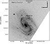 |
Fig. 1. Field of SN 2022jli in the i band observed with the LDSS-3 mounted at the Clay telescope at Las Campanas Observatory on May 22, 2022. The position of the SN is indicated in the figure. North is up and east is to the left. |
2.1. Photometry
We analysed public optical photometry from the Kleinkaroo Observatory reported by Monard to the TNS, from the Gaia mission2 (Gaia Collaboration 2016), from the ATLAS survey (Tonry et al. 2018; Smith et al. 2020), from the Zwicky Transient Facility (ZTF; Bellm et al. 2019), and from All-Sky Automated Survey for Supernovae (ASAS-SN; Shappee et al. 2014). We also present optical photometry obtained with the LDSS-3 instrument mounted to the 6.5-m Magellan Clay telescope, the EFOSC2 instrument with the 3.58-m New Technology Telescope (NTT), the Goodman instrument mounted on the 4.1 m SOAR telescope, and NIR photometry obtained with the Flamingos-2 instrument on the 8.1-m Gemini-South observatory. The optical photometry extends from a few days before maximum light to +418 days after maximum, and the NIR photometry extends from +38 days to +600 days.
2.1.1. Optical
To discount any potential issue in the public ZTF photometry of SN 2022jli, we downloaded the original ZTF images from the NASA/IPAC Infrared Science Archive3, and performed host-galaxy template image subtraction using HOTPANTS (Becker 2015). Aperture and PSF photometry was then computed from these template subtracted science images using PYTHON scripts. ATLAS forced photometry from the ATLAS forced photometry server was also downloaded and included in our analysis4. We include g-band ASAN-SN photometry to complement the photometry during the decline from the first maximum and on the rise to the second maximum. The ASAN-SN photometry correspond to photometry published by Moore et al. (2023) and Chen et al. (2024).
The reduction of the LDSS-3 and Goodman images was performed in IRAF following standard procedures that include bias subtraction and the normalisation of the science images using a normalised flat image, the astrometric registration of the images was done using ASTROMETRY.NET (Lang et al. 2010). The reduction of the EFOSC2 V-band acquisition image was done with the PESSTO pipeline (Smartt et al. 2015). Aperture and PSF photometry was performed with PYTHON scripts (see e.g., Hueichapan et al. 2022). The optical photometry of SN 2022jli is presented in Fig. 2. LDSS-3, EFOSC2 and Goodman photometry is reported in Table C.1 in the appendix.
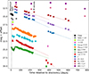 |
Fig. 2. Optical and NIR light curves of SN 2022jli. Circles correspond to survey photometry or NIR photometry repeatedly obtained using the same instrument or photometric system. Pentagons correspond to photometry computed from LDSS-3 and EFOSC2 spectroscopic acquisition images, diamonds are from late time Goodman photometry and triangles represent synthetic photometry computed from colour-matched spectra. The g-band photometry from ASAS-SN is shown using dark-green open circles to avoid confusion with other g-band photometry. The legend on the right specifies the colour code and the offsets employed to plot the different bands. Dotted lines are used to compare (extrapolate) the brightness decline from an early epoch to late times in a few relevant bands. |
2.1.2. Near-infrared
NIR photometry of SN 2022jli was obtained using the Flamingos-2 instrument (Eikenberry et al. 2004, 2012) mounted on the Gemini-South telescope. Flamingos-2 images were reduced using custom IRAF scripts. The reduction steps include the creation of a clean sky image, and the subtraction of this image from the science frames, flat fielding the science frames and the astrometric registration of the science images using ASTROMETRY.NET (Lang et al. 2010). The sky images were created from frames obtained in a position far from the host galaxy to avoid over subtraction of the host galaxy extended emission. The pre-explosion images of NGC 157 in JHKs obtained with the VIRCAM instrument (Dalton et al. 2006) mounted on the VISTA telescope (Emerson et al. 2006) at Paranal observatory were employed to subtract the host galaxy background emission from the SN images. The NIR photometry of SN 2022jli is reported in Table C.2 in the appendix, and shown in Fig. 2.
2.1.3. Mid-infrared
The field of the SN has been repeatedly visited by the Wide-field Infrared Survey Explorer (WISE) satellite (Wright et al. 2010) as part of the NEOWISE (Mainzer et al. 2011) and NEOWISE-R (Mainzer et al. 2014) missions. The NEOWISE-R mission observed the SN five times during 2022, 2023 and 2024. A careful inspection of the NEOWISE-R images before and after the SN explosion shows a clear mid-IR emission from the SN in the W1 and W2 bands, and no variability pre-SN explosion; therefore, pre-explosion images were used to subtract the host galaxy background emission from the images containing the SN. We obtained aperture photometry from host subtracted images. The NEOWISE W1 and W2 photometry is presented in Fig. 2 and summarised in Table C.3 in the appendix.
2.2. Spectroscopy
2.2.1. Optical
We obtained optical spectra of SN 2022jli with the LDSS-3 spectrograph mounted at the Clay telescope at Las Campanas Observatory, the Goodman spectrograph (Clemens et al. 2004) mounted at the SOAR telescope and the GMOS-S spectrograph (Hook et al. 2004; Gimeno et al. 2016) at the Gemini-South telescope. The LDSS-3 and Goodman data were reduced using IRAF routines. The reduction steps include bias subtraction, flat fielding, cosmic ray rejection using LACOSMIC (van Dokkum 2001), wavelength calibration, flux calibration and telluric correction. We performed the flux calibration and the telluric correction using a flux standard star observed on the same night of the SN spectra.
The GMOS-S spectra were reduced using the GEMINI IRAF package following standard reduction procedures similar to the ones described before, but using the GMOS IRAF task. The flux calibration was performed using a spectrophotometric standard star observed on a different night with the same instrument setup employed to observe the SN. The GMOS-S instrument is composed of three detectors, each one covering a different portion of the wavelength range. To obtain a continuous spectrum, almost free from the gaps between the detectors, two spectra of the SN shifted in wavelength were obtained5.
We include in our analysis the classification spectra reported to the TNS by Grzegorzek (2022) and by the ePESSTO+ collaboration. The ePESSTO+ classification spectrum is publicly available and was observed using the EFOSC2 instrument (Buzzoni et al. 1984; Snodgrass et al. 2008) mounted on the New-Technology Telescope (NTT) at La Silla observatory. The ePESSTO+ classification was independently reduced by our team using the PESSTO pipeline (Smartt et al. 2015). The optical spectra are presented in Fig. 3, and a summary of the optical spectroscopic observations of SN 2022jli is presented in Table 1.
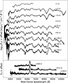 |
Fig. 3. Optical spectral sequence of SN 2022jli. The phase relative to the time of maximum light is indicated on the right. The spectra during the first +250 days are shown in the top panel in logarithmic scale, the nebular phase spectra are presented in the bottom panel. The smoothed nebular spectra using the Savitzky–Golay filter are shown in black, the original spectra are shown in grey. |
Summary of optical-wavelength spectroscopic observations of SN 2022jli.
2.2.2. Near-infrared
Seven epochs of NIR spectroscopy of SN 2022jli were obtained6 using the Flamingos-2 instrument (Eikenberry et al. 2004, 2012) mounted on the Gemini-South telescope. The observations were performed following an ABBA pattern, we observed the JH and HK configurations that cover from about 8750 to 17 000 Å and from 13 300 to 24 700 Å, respectively. We obtained a JH and HK pair as close in time as possible to obtain full NIR coverage.
One NIR spectrum of SN 2022jli was obtained using the fourth generation of the Triple-Spec spectrograph (Schlawin et al. 2014) mounted on the NIR Nasmyth platform of the SOAR telescope. Triple-Spec is a cross-dispersed, long-slit spectrograph with a resolution of about 3500, covering the full NIR wavelength range in one observation. The observations were performed following the ABBA pattern. The Triple-Spec spectra were reduced using its custom reduction pipeline, included in the SPEXTOOL IDL package (Cushing et al. 2004). We always observed an A0V telluric star before or after observing the SN and at a similar air mass. After the extraction of the individual spectra, we used the XTELLCORR task (Vacca et al. 2003) included in the SPEXTOOL IDL package (Cushing et al. 2004) to perform the telluric correction and flux calibration of the NIR spectra.
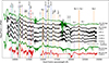 |
Fig. 4. NIR spectral sequence of SN 2022jli (in black) compared with SN 2013ge (in green; Drout et al. 2016) and SN 2011dh (in red; Ergon et al. 2015). The position of several lines are indicated with vertical lines and the phase relative to the maximum is indicated on the right. Five selected epochs are presented in this figure. |
Summary of NIR spectroscopic observations of SN 2022jli.
3. Analysis
3.1. Host galaxy
NGC 157 is an isolated SAB(rs)bc galaxy, with no close companions of comparable brightness detected in POSS images (Ryder et al. 1998). The galaxy heliocentric redshift is z = 0.005500 ± 0.000002 (from NED; Springob et al. 2005). The SN 2022jli is located in the north-west spiral arm of NGC 157. In this paper we adopt a distance of 23.5 ± 1.6 Mpc, corresponding to the distance derived from the host-galaxy recession velocity by NED considering a correction for Virgo, Great Attractor, and Shapley Supercluster infall (Mould et al. 2000), assuming H0 = 70.0 km s−1 Mpc−1.
3.2. Light curves
3.2.1. Epoch of maximum brightness
We used the unfiltered photometry obtained from the Kleinkaroo Observatory in South Africa and reported by Monard to the TNS to estimate the time of maximum light. In Fig. 5 we show the reported photometry fitted using a second order polynomial to estimate the SN 2022jli maximum brightness. From the polynomial fit we obtained that the epoch of maximum brightness (tmax) was on MJD = 59709.6 ± 1.2 days at an unfiltered brightness of 14.29 ± 0.02 mag, where the uncertainties are estimated using the covariance matrix of the polynomial fit. Conservatively, we assume an error on tmax equal to the time lapse between the discovery and the estimated epoch of maximum light, and an error on the brightness equal to the uncertainty on the closest photometric epoch, this is tmax = 59709.6 ± 5.4 days and 14.29 ± 0.05 mag. Hereafter we will refer to this epoch as the maximum time unless otherwise indicated. Our estimate of the epoch of maximum brightness is consistent with the phase reported based on the spectroscopic classification of Grzegorzek (2022).
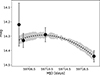 |
Fig. 5. Unfiltered photometry reported by Monard to the TNS obtained at the Kleinkaroo Observatory in South Africa (black points). The dotted black line corresponds to a second order polynomial fitted to the photometry. The polynomial fit was performed weighting by the photometric uncertainties and the shaded area corresponds to the 1σ uncertainty computed from the covariance matrix of the polynomial fit. From this fit we obtained that the epoch of maximum brightness was on MJD = 59709.6 ± 1.2 days at an unfiltered brightness of 14.29 ± 0.02 mag; however, we assume more conservative uncertainties for these parameters (see text). |
3.2.2. Secondary maximum and decline rates
SN 2022jli shows double-peaked light curves, and we estimate the epoch of the second maximum by fitting a low order polynomial to the photometry in the g, c and o bands. This procedure yields that the time second maximum took place on MJD equal to 59763.3 ± 8.8 days, 59752.4 ± 2.5 days and 59747.9 ± 1.4 days for the c, o and g bands, respectively. The time between the first and the second maximum is between +43 and +53 days, the minimum brightness in the g band was reached on 59724.4 ± 1.9 days, coincident with the minimum in the c band at about +20 days after the first maximum.
After the second maximum, the SN shows a linear decline which is well described by a linear polynomial fit. The average decline rate of the optical light curves in the time range between the MJD equal to 59790 and 59850 was measured, corresponding to a phase between +80 and +140 days relative to the first maximum. The uncertainties are estimated using the Monte Carlo methodology described in Cartier et al. (2022). The light curve decline rates are summarised in Table 3. The optical bands with bluer effective wavelengths (g and c bands), decline more slowly than the bands with redder effective wavelengths (r and o bands), at a significance of 8σ or higher. This is reflected in bluer optical colours at later times (see Section 3.2.5 below), meaning that the ejecta is continuously heated.
Summary of the linear decline rates of SN 2022jli.
From about +200 days the NIR light curves show a re-brightening (see Fig. 2). The NIR photometric coverage allow us to measure the light curve linear decline rate in two regions, in the MJD range between 59790 and 59900 days (+80 to +189 days; this is before the NIR re-brightening), and in the MJD range between 60090 and 60160 days (+378 and +448 days) at late times. These linear decline rates are also summarised in Table 3. The J band declines faster than the H and Ks bands. In concrete, the J band declines at a linear rate similar to the o band in the optical, while the Ks band decline rate is similar to the g band, this is before the onset of of the NIR re-brightening. Thus the linear decline rates in the NIR follow the opposite trend than the optical bands, this is a consequence of two different physical processes such as heating of the SN ejecta and dust emission.
At late times (> + 350 days) the decline rates in the NIR light curves in all bands are about 1 mag/100 days and are consistent with each other within the uncertainties, while the decline in the r band is about twice faster than the decline measured in the NIR bands.
The linear extrapolation from +80 to +189 days to late times shows that the SN is significantly brighter than the extrapolation in Ks (∼1.2 mag brighter), similarly the SN brightness in the H band is slightly fainter than the linear extrapolation (∼0.15 mag fainter), and the J band brightness is significantly fainter than the linear extrapolation (∼1.2 mag fainter).
3.2.3. Host-galaxy reddening
The Milky Way reddening in the direction of SN 2022jli is E(B − V)gal = 0.0383 (Schlafly & Finkbeiner 2011). The spectra of SN 2022jli are significantly reddened, showing a clear Na I D narrow absorption feature from the host-galaxy (see Fig. 6), implying that the SN suffers significant host-galaxy extinction. The pseudo equivalent width (hereafter EW) of Na I was measured in our highest signal-to-noise ratio spectra obtained at a phase before the host-galaxy Na I narrow line spectral region becomes too close to the edge of the underlying broad Na I spectral feature to be properly normalised. The spectra used to measure the Na I EW correspond to the LDSS-3, Goodman and GMOS-S spectra obtained at +11.7 days, +53.4 days, and +54.4 days, respectively (see Fig. 6). An average value of EW = 1.54 ± 0.12 Å was measured for the host Na I D1+D2 feature. Adopting the Poznanski et al. (2012) relation between the EW of the host Na I and colour excess, implies a host-galaxy colour excess of E(B − V)host = 0.9 ± 0.3 mag. Phillips et al. (2013) note that although a relation between the Na I EW and the extinction AV value exists, the uncertainty in AV from the Na I EW can be significant of the order of 0.3 dex, this is larger than the 0.08 dex quoted by Poznanski et al. (2012). Assuming the uncertainty of Phillips et al. (2013) we obtain E(B − V)host = 0.9 ± 0.7 mag. Since the Poznanski et al. (2012) relations are calibrated using the original Schlegel et al. (1998) extinction maps, we need to multiply the values derived from Poznanski et al. (2012) relations by 0.86 to place them in the re-calibration of Schlafly & Finkbeiner (2011), then the host galaxy reddening is E(B − V)host = 0.8 ± 0.6 mag from the Na I D1+D2 absorption feature.
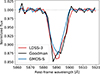 |
Fig. 6. Normalised host-galaxy Na I D line for SN 2022jli at +11.7 days (LDSS-3/Clay), +53.4 days (Goodman/SOAR) and +54.4 (Gemini-S/GMOS-S). The average equivalent width of the Na I D line for the three epochs is EW = 1.54 ± 0.12 Å. |
Drout et al. (2011) reported a small scatter of ±0.06 mag in the V − R colours of SE SNe (IIb/Ib/Ic) around +10 days relative to the V-band maximum. This property was latter confirmed by the radiative transfer models of Dessart et al. (2015) and investigated in detail by Stritzinger et al. (2018b) using multi-band photometry of SE SNe (Stritzinger et al. 2018a) from the Carnegie Supernova Project I (CSP-I; Hamuy et al. 2006). Using the CSP-I photometry, Stritzinger et al. (2018b) created unreddened colour templates for SE SNe, for the different sub-types (i.e. IIb, Ib, Ic). According to Stritzinger et al. (2018b) these templates can provide a host reddening estimate with photometry obtained between +0 to +20 days relative to V-band maximum.
We used the LDSS-3 and NTT (ePESSTO+) optical spectra of SN 2022jli obtained at +11.7 and +13.7 days, respectively, to compute synthetic colours. These spectra combined with the CSP-I broad-band transmission curves and zero points from Krisciunas et al. (2017), provide the colour information needed to estimate the SN reddening by means of computing synthetic photometry. As in Stritzinger et al. (2018b) and throughout this paper, the Fitzpatrick (1999) reddening law is adopted, and in this work RV = 3.1 is assumed. We also assume an uncertainty of 0.075 mag for the synthetic magnitudes, which translates to an uncertainty of 0.10 mag in colour. The total reddening along the line of sight (E(B − V)tot), which is the host galaxy and the Milky Way reddening, was inferred as the difference between the synthetic colours and the colour templates.
The reported colour excess value for each colour corresponds to the weighted average of the reddening values obtained for the two spectra. The quoted uncertainties were computed by adding in quadrature the uncertainties in the intrinsic colour-curve templates and in the synthetic colours. Table 4 lists our total and host-galaxy (E(B − Vhost)) colour excess estimations for SN 2022jli, inferred from nine colour combinations. We used the Fitzpatrick (1999) reddening law with RV = 3.1 to transform from a given colour excess to E(B − V) colour excess.
Summary of reddening determinations for SN 2022jli.
The host-galaxy reddening estimates derived from the Stritzinger et al. (2018b) colour templates yield values of E(B − V)host between 0.14 and 0.62 mag, with the E(B − g) colour being the most discrepant value of E(B − V)host = 0.62 ± 0.20 mag. Not considering the latter value, which seems to be an outlier, we obtain a weighted mean of E(B − V)host = 0.23 ± 0.06 mag, where the uncertainty is equal to standard deviation of the E(B − V)host values. Throughout the paper we assume E(B − V)host = 0.23 ± 0.06 mag for SN 2022jli, which when tacking on the MW reddening colour excess corresponds to a total value of E(B − V)tot = 0.27 ± 0.06 mag.
3.2.4. Periodicity in the light curves
After an inspection of the light curves of SN 2022jli, it was clear that in addition to the main re-brightening that occurs at 25-60 days after maximum light we could distinguish several softer bumps or undulations, which are clearly detected in the ATLAS and ZTF light curves. We fitted a fifth order polynomial to detrend the ZTF and ATLAS light curves to study the structure of these undulations. The polynomial fits were performed between +50 and +230 days relative to the first maximum. Polynomial fits using third or fourth order yield very similar results. For the analysis of the ATLAS light curves we consider observations with uncertainties smaller than 0.15 mag, and weighted averages were computed for the observations obtained within the same night (i.e. observed within 8 hrs difference), this procedure significantly reduces the noise of the ATLAS light curves.
The detrended residuals reveal periodic or quasi-periodic undulations, with the g band showing larger amplitudes than the r band. We found that the root mean square of the detrended g-band flux is 1.0 × 10⁻¹⁶ erg s−1 cm−2 Å−1 compared with 0.5 × 10⁻¹⁶ erg s−1 cm−2 Å−1 in the r band, confirming that the amplitude is larger in the bluer bands. We analysed the normalised light curve residuals using a Lomb-Scargle periodogram (see Fig. 7) to discover that the periodic signal is stronger in g than in the r band, with a period of 12.47 days and 12.27 days in the g and r bands, respectively. A similar analysis reveals a period of 12.71 days and 12.23 days in the c and o bands of ATLAS, respectively. Despite the small differences in the period found for the different bands, with bluer (g and c) bands having slightly longer periods than the redder bands (r and o), folding the ATLAS and ZTF light curves to a common period of 12.47 days they show a very good agreement in the periodic variability (see Fig. 8). This is consistent with Moore et al. (2023) and Chen et al. (2024) results; thus, we adopt this period hereafter in our analysis.
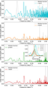 |
Fig. 7. Lomb-Scargle periodogram of the detrended and normalised g (green), r (red), c (cyan), and o (orange) light curves of SN 2022jli. The window functions are shown in grey for the different bands, and the inset shows in detail the region around the peak frequency. |
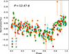 |
Fig. 8. Folded ATLAS and ZTF light curves to a common period of 12.47 days. |
3.2.5. Colour evolution
In Fig. 9 we present the g − r colours of SN 2022jli compared with the colours of the CSP-I SE SN sample Stritzinger et al. (2018a,b), the double-peaked SE SNe 2005bf (Folatelli et al. 2006), PTF11mnb (Taddia et al. 2018a), 2019cad (Gutiérrez et al. 2021), and 2019stc (Gomez et al. 2021). As could be expected, the synthetic colours of SN 2022jli at +12 and +14 days corrected for reddening (see Section 3.2.3) are located at the locus of the SE SNe intrinsic colour-curve evolution from maximum to +20 days.
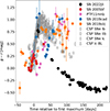 |
Fig. 9. g − r colours of SE SNe corrected by reddening using the Fitzpatrick (1999) reddening law. SN 2022jli is plotted in black, while in grey are the CSP-I SE SNe (Stritzinger et al. 2018b) with different symbols used for each SE SN sub-type as is indicated in the legend. For comparison are also presented the double-peaked SE SN 2005bf (Ib-pec; MJDmax = 53474.0; Folatelli et al. 2006), PTF11mnb (Ic-pec; MJDmax = 55827.4; Taddia et al. 2018a), SN 2019cad (Ic-pec; MJDmax = 58558.6; Gutiérrez et al. 2021) and SN 2019stc (Ic-pec; MJDmax = 58793.5; Gomez et al. 2021). |
As can be readily observed in Fig. 9, after the onset of the SN re-brightening (at 20 − 35 days), the SN displays very blue colours compared to the bulk of SE SNe. The SN is ∼0.65 mag bluer than the bulk of SE SNe at about +50 days. The SN continues evolving to bluer g − r colours until about +190 days after maximum, when a colour minimum is reached. Although all normal SE SNe tend to evolve from red to blue colour after reaching a peak in the g − r colour at about 25–30 days, the extreme colours of SN 2022jli are remarkable. The blue colour is presumably related with the extra power injection which produces the secondary maximum, increasing the ejecta temperature as we discuss in Section 3.2.7 below. If the SN 2022jli is not corrected by Galactic and host-galaxy reddening, the g − r colour of the SN would be ∼0.25 mag bluer than the bulk of the SE SNe. It is worth noting that SN 2022jli has bluer colours and higher ejecta temperature than the double-peaked SN 2019stc which follows a colour evolution comparable to the bulk of SE SNe. This suggests that the physical mechanism(s) producing the secondary maximum is probably different in these two SNe.
We note that the strong Na I D absorption line is readily noticeable throughout the SN evolution, suggesting that the dust and gas is not destroyed by the SN radiation, or by the potential ejecta-CSM interaction. Unfortunately, at late phases the Na I feature is located at the edge of an underlying broad spectral feature that prevents the most reliable measurement of its EW (see e.g., González-Gaitán et al. 2024).
In Fig. 10 we investigate the colour behaviour during the light curve undulations in detail. We present the total flux emission in the (g + r) bands corrected by reddening, compared with the g − r colours in two well-sampled regions of the ZTF light curves. We find that in addition to becoming blue with time, there is large scatter in the g − r colour showing periodic or quasi-periodic evolution. The peak to trough variation in the g − r colours is of the order of 0.07 to 0.10 mag, which is 5 − 7σ larger than the 0.015 mag variation expected from the median of colour photometric uncertainty alone. In Fig. 10, we mark the maxima of the (g + r) flux (dash-dotted blue line) and the peaks of the SN colours (dashed red lines), finding that at the epochs of flux maxima the SN tend to be bluer, while at the epochs of g − r colour peaks (redder colours) the SN is (generally) declining in (g + r) flux and close to a flux minima following a periodic or quasi-periodic cycle.
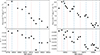 |
Fig. 10. Top panels: Total (g + r) flux corrected by reddening (E(B − V) = 0.27) following the Fitzpatrick (1999) reddening law for two regions with well-sampled light curves. Bottom panels: g − r colours (corrected by reddening) for the same two regions with well-sampled light curves. The vertical dash-dotted blue lines mark the observed flux maxima, and the vertical dashed red lines mark the colour maxima (redder colours). The flux and the colours show periodic undulations. |
3.2.6. Light curve comparison
In Fig. 11 the r-band absolute magnitude light curve of SN 2022jli is compared with the well observed SN 2011dh (Ib; Ergon et al. 2014, 2015), SN 2013ge (Ic; Drout et al. 2016) and the SE SNe from the CSP-I (Stritzinger et al. 2018a,b). The absolute magnitude at the first maximum of SN 2022jli is ≃ − 17.9 mag7 compared with the maxima absolute magnitude of ≃ − 17.2 mag of SNe 2011dh and 2013ge. As can be observed, SN 2022jli seems to be a bright SE SN, but within the range of normal luminosity objects. After the second maximum, the light curve of SN 2022jli is nearly parallel to the comparison objects, but with SN 2022jli is ∼2.3 mag brighter. At later times, SN 2022jli suffered a sudden luminosity drop between about +250 and +375 days (see also Chen et al. 2024), and by +400 days the SN spectrum (see Section 3.3.5 below) and brightness in the r band are similar to SN 2013ge.
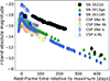 |
Fig. 11. Comparison between the r-band absolute magnitude of SN 2022jli (black symbols) and well-observed SE SNe from CSP-I (open symbols; Stritzinger et al. 2018b), SN 2011dh (blue diamonds; Ergon et al. 2015, 2014) and SN 2013ge (green triangles; Drout et al. 2016). SNe IIb, Ib, Ic and Ic-BL from the CSP-I are shown with open squares, pentagons, circles and triangles, respectively. |
3.2.7. Bolometric light curve
In Fig. 12 we present the pseudo-bolometric light curve of SN 2022jli. At early times during the first and secondary maximum, the scarcity of multi-band photometric observations poses a problem for the construction of a pseudo-bolometric light curve of SN 2022jli. We circumvent this problem by constructing spectral templates which are scaled in flux, using contemporary photometry to achieve an accurate flux calibration of the templates. The photometry used to scale the spectra was obtained as close in time as possible to the observing epoch of the spectra, usually in the same or within a couple of nights. In a few cases the photometry used to scale the spectra comes from the acquisition images of the spectra. At the minimum of the c band and the maximum of the o band we scaled template spectra with a time difference of 9 days and 12 days relative to the time of the photometry, respectively. We consider it important to have an estimate of the SN luminosity at these phases. In Section 3.3 we show that the spectra vary slowly during this time (from +14 to +55 days in Fig. 3). The uncertainty introduced by the use of spectra and photometry with a relevant time difference is accounted in the bolometric error (see Appendix). As is shown in Section 3.3 and in the Appendix, the spectrum of SN 2022jli after maximum light is similar to the spectra of SN 2013ge at a similar phase. We exploited this similarity to estimate the bolometric luminosity of SN 2022jli close to maximum light by employing the template spectrum of SN 2013ge at maximum. The maximum light spectral template of SN 2013ge was carefully colour-matched to the photometry of SN 2013ge and corrected by reddening along the line-of-sight to the SN. Then, the reddening free spectral template of SN 2013ge was reddened by the E(B − V) in the line-of-sight to SN 2022jli and scaled to the Gaia photometry of SN 2022jli close to maximum light (see the Appendix for more details). The pseudo bolometric luminosity of SN 2022jli is summarised in Table C.4.
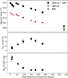 |
Fig. 12. Top: pseudo-bolometric light curve of SN 2022jli (black circles) computed integrating the SN spectra in the optical region between 3800 and 9000 Å (green pentagons) and taking in account the NIR contribution (red pentagons). The NIR emission during the decline from the first maximum was estimated from optical+NIR templates of SN 2013ge as described in the text, and these estimates are shown using open pentagons. The pseudo-bolometric luminosity at +383 days was estimated directly from the griJHKs photometry. Middle: Tbb computed from a black-body fit to the spectra of SN 2022jli. Bottom: Rbb from a black-body fit to the spectra of SN 2022jli. |
We estimate the NIR contribution at the first maximum and during the decline from it using spectrophotometric templates of SN 2013ge. These optical-NIR templates were constructed by colour matching the optical spectra to the photometry, and the NIR spectra were scaled to the optical spectra in their overlapping regions (from 8000 to 9500 Å approximately). We estimate that the NIR contribution is of the order of 10 − 15% of the total optical and NIR emission during this phase. From +38 days the NIR contribution was estimated directly from the NIR photometry of SN 2022jli, and is of the order of 7 − 9% until ∼230 days. At about +380 days the NIR corresponds to 59% of the SN emission.
The bolometric light curve of SN 2022jli is double-peaked, with both maxima reaching a similar bolometric luminosity of about 3 × 1042 erg s−18. The estimated decline rate from the first maximum is 3.67 ± 0.94 mag/100 days, and the decline rate after the second maximum is 1.18 ± 0.10 mag/100 days. At later times the SN showed a significant drop in luminosity, and the pseudo-bolometric luminosity becomes dominated by the NIR emission (corresponding to 60%).
A black-body model was fitted to the optical spectra of SN 2022jli after scaling them and matching their colours to the photometry. The estimated black-body temperature (Tbb) and radius (Rbb) are shown in Fig. 12. During the decline from the first maximum the ejecta temperature is ∼5000 K and Rbb ≃ 2.7 × 1015 cm (≃39 000 R⊙). After the second maximum the ejecta temperature increases and the Rbb shows a decrease with time reaching a minimum of Rbb ≃ 6 × 1014 cm (≃8600 R⊙) at about +150 days and staying constant thereafter. The ejecta temperature reaches a maximum temperature of ≃9000 K at about +150 days, and the ejecta temperature decreases thereafter.
3.2.8. 56Ni and ejecta mass
In order to estimate the mass of the ejecta (Mej) and of the radioactive 56Ni (MNi) produced by the SN, we used the Arnett (1982) analytical solution for type I SNe, assuming that the first maximum is powered by the radioactive decay of 56Ni and employing the methodology described in Cartier et al. (2022). We fitted the bolometric light curve of SN 2022jli from the first maximum to the minimum at about +20 days, assuming an ejecta velocity at maximum light of vej = 8500 km s−1 (see Section 3.3.4), an optical opacity of κ = 0.07 cm2 gr−1 and a rise time to maximum light of τrise = 14 days. This rise time provides the best fit to the bolometric light curve measured using the reduced χ2. The rise time to maximum calculated for SN 2022jli is also consistent with the typical rise times measured in normal SNe Ic. For example, Taddia et al. (2015) reports average rise times in the r band of 22.9 ± 0.8 days, 21.3 ± 0.4 days, 11.5 ± 0.5 days and 14.7 ± 0.2 days for SNe IIb, Ib, Ic and Ic-BL from SDSS-II, respectively. Although Arnett’s analytical solution has limitations (see e.g., Khatami & Kasen 2019; Afsariardchi et al. 2021; Rodríguez et al. 2023), like the assumption of a constant optical opacity, Arnett’s model remains a widely used, simple, and powerful analytical model to obtain reasonable estimates for Mej and MNi. Other methodologies cannot be used to estimate the MNi because; i) the time of the explosion is not well constrained from the observations, ii) the lack of multi-band photometry during the rise to the first maximum, and iii) only one (pseudo) bolometric epoch is available at late times when the power source that produced the second maximum had significantly decreased. Following Taddia et al. (2018b), it is assumed κ = 0.07 cm2 gr−1, since it provides consistent results for the Mej and MNi parameters when Arnett’s analytical model is compared with the hydro-dynamical models of Bersten et al. (2011, 2012), both fitted to the bolometric light curves of the CSP-I sample (see Taddia et al. 2018b, for a discussion).
Figure 13 presents the analytical fit to the first bolometric peak of SN 2022jli. Given that the rise to maximum of SN 2022jli is not constrained, we explored a range of τrise from +10 to +23 days, which comprises the range of typical τrise found in SNe Ibc (see Taddia et al. 2015). It was found that 14 days provides the best analytical fit for SN 2022jli, with good fits having τrise in the range of 11 to 17 days. In this range of τrise the analytic solution provides an ejecta mass (Mej) and a radioactive 56Ni mass (MNi) that do not significantly vary. The values obtained for SN 2022jli are Mej ∼ 1.5 ± 0.4 M⊙MNi ∼ 0.12 ± 0.01 M⊙, where the quoted errors reflect the uncertainty in the assumed τrise and vej. The good quality of the fit to the first maximum of the bolometric light curve, the fact that Mej and MNi are typical of a standard SN Ic and that SN 2022jli shows spectral features of a SN Ic, supports the idea that the first maximum of SN 2022jli is a standard SN Ic mainly powered by the decay of 56Ni.
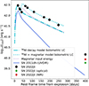 |
Fig. 13. Fit of the radioactive decay of 56Ni to the first maximum of the bolometric light curve of SN 2022jli, using the Arnett (1982) analytic approximation. The parameters of the best-fit model are τrise = 14 days, Mej ∼ 1.5 M⊙, MNi ∼ 0.12 M⊙, vej = 8500 km s−1 and κ = 0.07 cm2 gr−1. This model illustrates that the first maximum of SN 2022jli is consistent with the typical rise time, 56Ni and ejecta mass of a normal SN Ic. The estimated MJD of the explosion is 59695.4 days. The secondary maximum is modelled as the sum of the radioactive decay of 56Ni and the spin-down energy from a magnetar (dotted cyan line; see Cartier et al. 2022, for details about the magnetar model). To model the secondary maximum the magnetar birth is delayed 37 days relative to the assumed time of the SN explosion and the magnetar parameters are B ∼ 8.5 × 10¹⁴ G and P ∼ 48 ms. The dotted purple line shows the magnetar contribution to the bolometric light curve. The optical and NIR luminosity at +383 days are shown using green and red pentagons, respectively. The pseudo-bolometric (UVOIR) light curve of the well-observed SE SN 2011dh (IIb) is shown for comparison (MNi = 0.075 M⊙; Ergon et al. 2015). |
As was noted previously, at later times the SN shows a drop in luminosity, which marks a decrease in the power injection from the energy source producing the second maximum. This might be a consequence of the well known drop in the ejecta opacity to γ-rays at late times, due to the expansion of the SN ejecta. This is illustrated in Fig. 13 with the rapid decline of the UVOIR light curve of SN 2011dh (Ergon et al. 2015) after maximum light. SN 2011dh is chosen for comparison because is a normal SE SN (type IIb) with a high-quality and well-sampled UVOIR light curve, constructed from high-quality and well-sampled optical and IR observations from the U band to the mid-IR SpitzerS2 band collected from +4 days until about +400 days. SN 2011dh has an estimated MNi = 0.075 M⊙, and its decline rate after maximum is significantly faster than the decline rate expected of full trapping from the 56Co decay, the daughter product of 56Ni. As in the case of SN 2011dh, a significant fraction of the power from the 56Co radioactive decay probably escape after maximum in SN 2021jli9.
3.3. Spectra
3.3.1. Spectral comparison
In Fig. 14, SN 2022jli is compared with other SE SNe at about +12 days, during the decline from maximum brightness and before its re-brightening. SE SNe are classified as Type IIb, Type Ib and Type Ic depending on the presence of clear and unambiguously detectable amounts of hydrogen and helium in the SN ejecta. At this phase, the spectral features of SN 2022jli correspond to a SN Ic very similar to SN 2013ge during its decline from maximum light. The spectra of SN 2022jli do not show strong helium or Balmer absorption lines such as in SN 2007Y (Ib) and in SN 2011dh (IIb). A comparison with the bumpy SLSN-I SN 2019stc shows that this SLSNe exhibit a bluer continuum and broader spectral lines yielding more blended spectral features compared to their lower luminosity cousins like SN 2022jli.
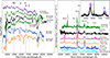 |
Fig. 14. Comparison of SN 2022jli with other SE SNe in decline from the first maximum and at a late nebular phase. On the left panel, SN 2022jli is compared at about +12 days relative to the first maximum, during the decline from maximum light, with the bumpy SLSNe-I SN 2019stc (Gomez et al. 2021), the Ic SN 2013ge (Drout et al. 2016), the Ib SN 2007Y (Stritzinger et al. 2009, 2023) and the IIb SN 2011dh (Ergon et al. 2014). The black tick marks the Na I D feature which is strong in SN 2022jli possibly due to the He Iλ5876 line contribution. Similarly, on the right panel, SN 2022jli is compared with the SLSN-I SN 2015bn (Nicholl et al. 2016a), the Ic-BL SN 2002ap (Shivvers et al. 2019), SN 2013ge and SN 2011dh (Ergon et al. 2015) at nebular phase. We indicate the rest-frame wavelength of the main spectral features. All the spectra have been corrected for reddening assuming RV = 3.1 and values from the literature, in the case of SN 2022jli we assume E(B − V)tot = 0.27 mag. |
A manifestation that the envelope stripping is probably not complete is that some SNe Ib exhibit small amounts of hydrogen material (see e.g., Holmbo et al. 2023; Dong et al. 2024) and some SNe Ic show evidence of helium in their ejecta (see e.g., Drout et al. 2016; Shahbandeh et al. 2022; Holmbo et al. 2023). This is also the case of SN 2013ge that although it is classified as a SN Ic, it shows weak He I features in the optical and in the NIR (see Drout et al. 2016) and has an estimated ejecta mass of 2–3 M⊙, not far from the estimated ejecta mass of SN 2022jli. Similarly, SN 2022jli also shows weak He I features as discussed below (see also Moore et al. 2023). Additionally, a double-peaked, weak and variable Hα feature is robustly detected after the second maximum. This spectral feature shows a periodic shift in its peak following the light curve undulations and it seems to be a manifestation of the accretion of hydrogen-rich material from a companion star in a binary system (Chen et al. 2024). The Ic classification of SN 2022jli is reinforced by its nebular spectrum (see Fig. 14); this is discussed in detail below.
Close to the time of the second maximum, the spectral features of SN 2022jli do not show a significant evolution (see Fig. 15). At this phase, the spectrum of SN 2022jli still shows a clear pseudo-continuum, and a few (pseudo-)nebular features begin to appear in the red part of the optical spectrum, such as [Ca II] λλ7291, 7323 and O Iλ7774. In turn, the spectral features in the blue part of the optical region (< 7000 Å) remain essentially the same, and remain almost unaltered for the next 100 days, evolving very slowly.
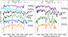 |
Fig. 15. Comparison of SN 2022jli with other SE SNe during the SN re-brightening. On the left panel, the SN is compared at the time of its second maximum with the SLSNe-I SN 2019stc (Gomez et al. 2021) and SN 2015bn (Nicholl et al. 2016b), the Ic SN 2013ge (Drout et al. 2016), the Ib SN 2007Y (Stritzinger et al. 2009, 2023) and the IIb SN 2011dh (Ergon et al. 2014) at a similar phase relative to the first maximum. Similarly, on the right panel, SN 2022jli is compared with SN 2019stc, SN 2013ge and SN 2011dh (Ergon et al. 2015) at about +149 days relative to the first maximum. We indicate the rest-frame wavelength of the main spectral features. All the spectra have been corrected for reddening assuming RV = 3.1 and values from the literature, in the case of SN 2022jli we assume E(B − V)tot = 0.27 mag. |
Between +45 and +65 days, normal SNe Ic become pseudo-nebular, the continuum emission decreases and becomes redder. Spectral features of [Ca II] λλ7291, 7323, and a strong Ca II NIR P-Cygni emission are clearly present, and a weak [O I] λλ6300, 6364 feature can be distinguished. In turn, the Ca II NIR triplet in SN 2022jli is shallower than in the comparison SE SNe, and even compared with the same SN during its decline from the first maximum. All of this is a consequence of the extra energy input which makes the pseudo continuum bluer compared with other SE SNe. The [O I] λλ6300, 6364 doublet is absent in SN 2022jli at this epoch, and it may weakly contribute to the SN spectrum after +150 days. However, the [O I] doublet seems to appear after +200 days in the SN spectrum and it becomes the strongest optical spectral feature by +400 days (see Fig. 14).
In the right panel of Fig. 15 we compare SN 2022jli with other SE SNe at 150 days. At this phase SN 2022jli is becoming pseudo-nebular, a decrease in the continuum can be appreciated at wavelengths redder that 5500 Å, but the continuum remains bluer than that of normal luminosity SE SNe, its continuum shape is more similar to SLSNe-Ic. The shape of the spectral features, on the other hand, is more similar to SE SNe rather than to SLSNe. For comparison, at this phase SE SNe are nebular, showing [O I] λλ6300, 6364 and [Ca II] λλ7291, 7323 lines (see Fig. 15).
In summary the evolution of the optical spectra of SN 2022jli after the re-brightening resembles the evolution of SLSNe-I in the sense that these SNe show a slow evolution and bluer continuum compared to normal luminosity SE SNe. However, SN 2022jli has stronger spectral features typical of a SN Ic, whereas SLSNe-Ic have shallower and broader spectral features (see Fig. 15 and Cartier et al. 2022, for a discussion). The spectral features displayed by SN 2022jli and by all normal SNe Ic show less blending than most SLSNe-Ic, pointing to a less energetic explosion of SN 2022jli than SLSNe-Ic.
Presented in Fig. 4 is the NIR spectral sequence of SN 2022jli starting at +38 days relative to the first maximum and continuing for nearly +200 days. As in the optical, SN 2022jli evolves slowly in the NIR. We identify strong lines of O I, C I, Mg I, Mg II, Na I, weak lines of He Iλ2.058 and Paβ as is discussed below, and potential lines of Si I. Weak lines of [Fe II] seem to appear between 100 and 200 days, these lines are commonly observed in most core-collapse SNe. Initially, at +38 days, we identify that the strongest spectral features in the H and Ks bands correspond to Mg II. As the Mg II lines fade, the Mg I spectral features become stronger.
3.3.2. Helium
The optical spectra of SN 2022jli do not show unambiguous He I lines, but the potential presence of a small amounts of helium is suggested by the strong absorption feature at about 5730 Å, which is usually associated with the Na I D line in SNe Ic, but in this case the absorption feature seems to be strengthened by presence of the He Iλ5875 line (see Fig. 14). In addition, a weak spectral feature coincident with He Iλ7065 from about ∼ + 50 days (see Fig. 15) also suggests the presence of small amounts of helium. The existence of helium is the SN ejecta is further supported by a very weak broad spectral feature barely detected at ∼2.058 μm in the NIR spectra at +36 and +92 days (see also Tinyanont et al. 2024). As is discussed in Dessart et al. (2020) and Shahbandeh et al. (2022), the He Iλ2.058 line is probably the best suited spectral feature for an unambiguous detection of helium in SNe Ic.
3.3.3. Hydrogen
SN 2022jli shows a broad and blended spectral feature at the location of Hα (Fig. 16), and a double-peaked profile at the location of the Paβ (Fig. 17). From about the time of the second maximum the Hα feature begins to show a double-peaked profile (see Fig. 16). The peaks of the double horned profiles in the Hα and Paβ features are located at about ±1000 km s−1 from the central rest-frame line position (see Figs. 16 and 17).
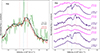 |
Fig. 16. Velocity profile of the region around the Hα spectral feature. A pseudo-continuum on each side of the profile has been used to subtract the underlying continuum emission, and the result was normalised by the median residual flux over the region. On the left panel, the spectral region of SN 2022jli during the decline from the first maximum is compared with SN 2013ge (in green) at a similar spectral phase of ∼12 − 14 days. On the right hand panel, the evolution of the Hα velocity profiles of SN 2022jli from +53 days to +232 days are shown, during and after the second maximum, ordered with respect to the phase folded period of 12.472 days (ϕ). The near-maximum spectra are shown in magenta, the intermediate-phase spectrum at +92.1 days spectrum is shown in dark magenta, and the late-phase spectra (> + 100 days) is shown in indigo. The phase with respect to maximum and the periodic phase (ϕ) are indicated on the right of each spectrum. Vertical dotted red lines indicate a velocity of ±1000 km s−1 for comparison. |
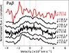 |
Fig. 17. Velocity profile of the region around the Paβ spectral feature in the NIR. As in the case of Hα, a pseudo-continuum on each side of the profile has been used to subtract the underlying continuum emission, and the result was normalised by the median residual flux over the region. Vertical dotted red lines indicate a velocity of ±1000 km s−1 for comparison. |
The evolution of the Hα profile is presented in Fig. 16. A pseudo-continuum on each side of the profile has been used to subtract the underlying continuum emission, and the resulting residuals were normalised by the median residual flux over the region. In the left panel, the spectra at +12 and +14 days are compared with the spectra of SN 2013ge at a similar phase. There is a potential excess emission at ∼ + 800 km s−1; however, the overall profile is very similar to the profile of SN 2013ge and no clear evolution in the shape of the spectral feature is detected between the two epochs. Therefore the presence of Hα emission is ambiguous during the decline from the first maximum.
In the right panel, the Hα profiles from about the time of the second maximum until +232 days are presented, ordered by phase assuming a period of 12.47 days. The spectra obtained close to the secondary maximum (53–55 days) and at +92.2 days (ϕ in the range of 0.28 − 0.44) show a double-peaked profile similar to the one first detected at +92.1 days in the Paβ line, but there is no apparent shift in the line profiles over this phase. In the spectra at > + 100 days, the double-peaked feature becomes more conspicuous and shows a clear shift in the peak position with phase. The latter is probably due to the larger phase coverage in the spectra after 100 days (ϕ from 0.30 to 0.94).
The Paβ profile is not detected in the NIR spectrum at +38.5 days, and only becomes evident in the spectrum at +92.2 days (see Fig. 17), after the time of the secondary maximum. The feature becomes more conspicuous with time, as can be observed in Fig. 4. The maxima of the double-peaked profile seem to shift as a function of the phase of the periodic undulations and consistent with the variation observed in the Hα feature at > + 100 days (Fig. 17). No other hydrogen lines are clearly detected in the NIR spectra of SN 2022jli. Furthermore, we inspected in detail the region of Brγ and the line is not visible despite the high signal-to-noise ratio of the NIR spectra. Some weak hydrogen lines may be blended with lines of other species. The Hα and the Paβ lines produce relatively weak spectral features indicative of a small amount of hydrogen, and the double-peaked profiles could be a consequence of an accretion disc or of out-flowing material ejected in winds. At +400 days the SN spectrum is fully nebular and spectral feature associated with Hα is no longer detected, supporting the conclusion that the amount of hydrogen material mixed in the ejecta is very small, if any.
Narrow Hα emission lines (FWHM = 3.5 − 6.5 Å) are present in the nebular spectra obtained with the GMOS-S and LDSS-3 spectrographs at late times, this narrow emission is not present in the nebular spectrum obtained a few days before with the Goodman spectrograph. A careful inspection of the 2D spectra shows strong narrow Hα and [N II] emission lines from the host galaxy, where the Hα line is coincident with a night sky line. In addition, on the 2D spectra the Hα emission has irregular structure in the spatial direction, and small shifts (< 5 Å) due to the galaxy rotation in the dispersion axis. We suspect that the narrow Hα feature is most likely due to an incomplete subtraction of the host galaxy Hα background emission close to the SN. This is supported by the small FWHM measured from the Hα narrow feature in the GMOS-S spectrum, which is half the instrument resolution. Thus, probably originates from an imperfect subtraction. However, we are cautious, and the potential appearance of late time narrow hydrogen lines such as in SN 2016adj (Stritzinger et al. 2024) cannot be completely discounted.
3.3.4. Expansion velocity
As was previously discussed, SN 2022jli shows spectral features of a SN Ic after maximum light and throughout its evolution. Now we pay attention to the ejecta expansion velocity. We estimate the ejecta velocity from the minimum of the Fe IIλ4923.9, Fe IIλ5001.9 and Fe IIλ5169.0 absorption lines. In Table 5 we summarise the ejecta velocity estimated from each of these three lines, and provide their weighted average. The uncertainty of the weighted average corresponds to the maximum value between the error from the weighted mean and the standard deviation from the three independent measurements.
Summary of the Fe II expansion velocity of SN 2022jli.
Figure 18 compares the ejecta expansion velocity of SN 2022jli with the normal type Ic SN 2007gr and SN 2013ge. For these three SNe, the ejecta velocity was estimated using the Fe II lines. Taddia et al. (2018b) shows that the Fe II velocity evolution from early times, before maximum light, to late times can be described with a power law. Here we show that from about +10 days the ejecta velocity is well described by a linear decline, assuming that the velocity decline rate for these three SNe was measured in a time window between +10 and +100 days. We found that the velocity decline rates are 13.5 ± 0.8 km s−1 day−1 for SN 2022jli, 44.9 ± 5.8 km s−1 day−1 for SN 2013ge and 17.0 ± 0.6 km s−1 day−1 for SN 2007gr. The expansion velocity of SN 2022jli after maximum is comparable to other SNe Ic, and extrapolating linearly its velocity to maximum light a value of  km s−1 is obtained, the true value must be slightly higher given the power-law behaviour of the ejecta velocity at early times. The velocity decline rate post-maximum of SN 2022jli follows a linear evolution marginally slower than the comparison SNe. The latter suggest that the physical mechanism producing the secondary maximum and the undulations has a moderate effect on the expansion velocity of the ejecta. Arguably the main effect is to inject energy to the ejecta keeping a pseudo-photosphere for longer time at a higher ejecta velocity compared with normal SNe Ic. The latter effect is evident at about 100 d, when the comparison SNe Ic are almost fully nebular, and the non-nebular Fe II lines are no longer detected. The linear extrapolations of the ejecta velocities of the comparison Ic’s at +100 days are slower (≤6000 km s−1) than the ejecta velocity of SN 2022jli at this phase (≃7000 km s−1).
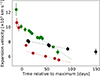 |
Fig. 18. Expansion velocity estimated from the Fe II lines (see text) for SN 2022jli (black), SN 2013ge (green) and SN 2007gr (red). The dashed lines illustrate the velocity decline rate, measured between +10 and +100 d, for the three SNe. |
3.3.5. Nebular phase
In Fig. 14 the spectrum of SN 2022jli at +418 days is compared with the spectra of other SE SNe at nebular phase. SN 2022jli appears like a normal SN Ic similar to SN 2013ge. The strongest spectral features of SE SNe at this phase are the [O I] λλ6300, 6364 and [Ca II] λλ7291, 7323 lines.
The [O I] and [Ca II] emission lines are studied using Gaussian profiles to fit the lines. The continuum emission regions were defined selecting the minimum on each side of the spectral features, and a linear polynomial was fitted between these regions to subtract the continuum emission. In SN 2022jli, the [O I] line does not show any contamination from other broad features such as Hα or [N II], as is frequent in Type IIb and Ib SNe (see e.g., SNe 2011dh and 2007Y in Fig. 14). The [O I] doublet was modelled using two Gaussian profiles fixing the ratio between the to components to 3:1, assuming an optically thin nebular emission as in Taubenberger et al. (2009). The [Ca II] lines show a weak but clear contamination from the [Fe II] λ7155 line on the blue part of the profile, and can also be contaminated by other relatively weak [Fe II] and [Ni II] lines in this region. We assumed that the [Fe II] λ7155 emission can be well described by a Gaussian profile, the profile was fitted using blue part of the [Fe II] λ7155 line, which does not seem to be affected by the [Ca II] emission. Making use of the Gaussian fit, the flux contribution from the [Fe II] λ7155 line was subtracted from the [Ca II] spectral feature.
The [O I] emission line of SN 2022jli does not require an additional component, and it does not show a double-peaked profile found in some SE SNe (see e.g., Maeda et al. 2008; Taubenberger et al. 2009; Fang et al. 2022; Prentice et al. 2022). In Table 6 we summarise the central velocity of the [O I] (v[O I]) and the [Ca II] (v[Ca II] ) doublets, their FWHM, and the [O I]/[Ca II] flux ratio. The [Ca II] line in the +412 days GMOS spectrum is affected by gap of ∼100 Å on the red tail of the spectral feature (see Section 2.2). We present the measurements of the SN 2013ge nebular spectrum for comparison.
Summary of nebular phase spectroscopic measurements.
Prentice et al. (2022) studied the [O I]/[Ca II] ratio for a sample 86 SNe from the literature, finding that this ratio does not evolve significantly between about +200 days and +400 days in normal luminosity CC SNe. The different sub-types are found in a well-localised range of values. For example, SNe II have [O I]/[Ca II] ratios in the range 0.3 − 1.4 with a median 0.5, SNe IIb are found in the range of 0.5 − 3.3, SNe Ibc in the range of 1.0 − 5.0, while SLSNe-I are found in a wide range of values overlapping with II and IIb SNe. The [O I]/[Ca II] = 2.2 ± 0.1 for SN 2022jli confirms its SE SN nature, and places this object within the Ibc range.
3.4. Carbon monoxide emission and late-time near-infrared excess
The formation of carbon monoxide (CO) is key in the process of molecule and dust formation in the SN ejecta, playing an important role in cooling the SN ejecta (Liljegren et al. 2020) to temperatures at which dust can form, and key in the chemical reactions leading to complex molecule formation. The CO molecule is readily detectable in late time NIR spectra of SNe from its first CO overtone emission in the spectral region between 2.3 and 2.5 μm (e.g., Spyromilio et al. 1988; Elias et al. 1988; Gerardy et al. 2002; Hunter et al. 2009; Drout et al. 2016; Banerjee et al. 2018; Rho et al. 2018, 2021; Tinyanont et al. 2019; Stritzinger et al. 2024; Park et al. 2025; Hueichapán et al. 2025a). The fundamental CO mode at about 4.6 μm is frequently detected in the small number of CC SNe observed at late-times in the mid-IR (e.g., SN 1987A, SN 2004dj, SN 2004et, SN 2005af and SN 2017eaw; see Catchpole et al. 1988; Meikle et al. 1989; Kotak et al. 2005, 2006, 2009; Szalai et al. 2011; Tinyanont et al. 2019; Dessart et al. 2025; Medler et al. 2025; Jacobson-Galán et al. 2025).
In Fig. 19 the first CO overtone spectral feature of SN 2022jli is compared with other CC SNe with clear first CO overtone emission. The first CO overtone feature is detected for first time in SN 2022jli at +190 days, where the CO overtone band-heads can be clearly distinguished (see Fig. 19). Compared with other CC SNe, the first CO overtone emission in SN 2022jli is relatively weak, and it is significantly weaker than in the type Ic SN 2013ge, and similar to the first CO emission of SN 2016adj. The potential detection of CO emission at earlier times is ambiguous. For example, at +139 days we can distinguish a broad spectral feature at the expected location, but it seem to be dominated by the emission from the Mg IIλ24048 line and the characteristic CO band-heads are not distinguishable. At around 400 days the first CO emission is no longer detected in SN 2022jli, at this phase the Ks band is dominated by dust thermal emission (see Fig. 20).
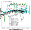 |
Fig. 19. Comparison of the first CO overtone region of SN 2022jli at +139, +190 and +224 days with the with nebular phase CO emission from the type Ic SNe 2013ge (Drout et al. 2016) and SN 2016adj (Stritzinger et al. 2024), and the type II SNe 1987A (Bouchet et al. 1991), 2017eaw (Rho et al. 2018) and 2020ocz (Cartier et al. 2021). The phase and the SN colour are indicated in the inset. |
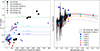 |
Fig. 20. Left panel: H − Ks colour evolution of SN 2022jli (black circles) compared with the colour evolution of the type Ic SN 2016adj (teal X symbols; Stritzinger et al. 2024), SLSN 2015bn (cyan pentagons; Nicholl et al. 2016b), type IIb SN 2011dh (blue diamonds; Ergon et al. 2014, 2015), the type Ic SN 2007gr (red hexagons; Hunter et al. 2009) and the type IIn SN 2005ip (purple plus sign; Stritzinger et al. 2012). The horizontal dashed lines correspond to the H − Ks colour of a given black-body temperature as indicated in the figure for comparison. Right panel: Evolution of the NIR SED of SN 2022jli from +238 to +600 days. A full NIR spectrum of SN 2022jli at around +422 days is presented, and for comparison a black-body SED having T = 945 K is presented for comparison (dashed red line). The dotted lines correspond to dust SED fitting results to the H, Ks and W1 photometry of graphite dust with a radius of 0.1 Å, using the Qabs from Draine (2016). |
The IR photometry of SN 2022jli reveals a flattening in the JHKsW1W2 emission at around 200 days (see Fig. 2), which is more evident in the redder IR bands. This IR-excess in SN 2022jli is illustrated in the H − Ks colour diagram of Fig. 20, where a jump in the H − Ks colour of ∼0.35 mag between +180 and +238 days marks the onset of strong dust emission. The SN continues evolving to extremely red H − Ks colours over the course of the following year, which is a consequence of the dust cooling and of the predominance of the dust thermal emission over the SN ejecta emission.
As is shown in the right panel of Fig. 20, despite the red SN colour, the SN emission in the J and H bands at +238 days is still dominated by the SN ejecta emission. Five months later, at a phase of about +380 days, the ejecta emission has significantly faded and the NIR emission is now dominated by thermal dust emission (see Fig. 20). A NIR spectrum at around +420 days, reveals that the J band still displays broad nebular spectral features from the SN ejecta; however, the emission in the H and Ks bands is dominated by dust thermal emission.
Assuming optically thin dust emission, we fitted the H, Ks, and W1 (when available) photometry using the expression
 (1)
(1)
where κν(a), the dust mass absorption coefficient, is
 (2)
(2)
Here a is the dust radius, ρ is the dust density, and Qa is the dust absorption efficiency. Here we study two cases: a single-crystal size graphite dust composition for which the Qa was computed by Draine (2016) using the discrete dipole approximation, and a single-size silicate dust composition (forsterite) with the Qa computed using the 1/3–2/3 approximation (Draine & Lee 1984; Laor & Draine 1993). The W2 band shows an excess of emission compared with the dust models for both compositions, this band is probably affected by the emission from the fundamental CO band which is coincident with the effective wavelength of the W2 band (4.6 μm) and is not included in the fits10. The evolution of the graphite and silicate dust temperature (Td), mass (Md) and luminosity (Ld) for SN 2022jli assuming a dust radius of a = 0.1 Å are presented in Fig. 21. In this figure, a decrease in Td and Ld parameters can be observed with time. This trend in the evolution is independent of the dust size and composition assumed. The weighted mean for Md is 2.5 ± 1.3 × 10⁻⁴ M⊙ for graphite dust and 10.1 ± 3.0 × 10⁻⁴ M⊙ for forsterite silicate dust, both for single-size crystals of a radius of a = 0.1 μm. In the fitting of the photometry we consider a significant range in the dust radius, finding that for dust particles with a radius a ≤ 0.2 μm variations of < 20% in Md are observed. When larger dust radii are considered a ≥ 0.3 μm the Md is scaled down by a factor of ∼0.5 compared with the reference radius of a = 0.1 μm for both dust compositions, graphite and silicate.
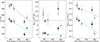 |
Fig. 21. Evolution of the dust temperature, mass, and luminosity as a function of time relative to maximum light for silicate (triangles) and graphite (circles) dust, assuming a dust radius of 0.1 μm. Black symbols correspond to fits performed to H, Ks, and W1 photometry and grey symbols to fits performed using only H and Ks photometry. Dotted magenta and cyan lines correspond to linear fits to Td and log10(Ld) for silicate and graphite dust, respectively. The horizontal dotted cyan and magenta lines indicate the weighted means for Md of 2.5 ± 1.3 × 10⁻⁴ M⊙ and 10.1 ± 3.0 × 10⁻⁴ M⊙ for graphite and silicate dust, respectively. |
We considered the Md evolution in more detail. In the case of dust formation in the SN ejecta Md usually increases with time. An increase in Md with time is observed in the fits that include W1-band photometry (black symbols in Fig. 21), while a decreasing trend in Md is observed in the fits performed using only H65nd Ks photometry. The inclusion of W1 photometry practically does not alter our estimates, but reduce significantly the uncertainty, in particular in the fits at +570 days. The observed decrease in Md in the fits performed to only the H and Ks bands is largely due to the last measurement, with a difference between the first and the last (minimum) value of 1.8σ, independent of the dust radius and composition assumed. Future IR observations of SN 2022jli with the James Webb Space Telescope (JWST) are key to constrain the dust composition of the emitting dust, to reveal the presence of more than one dust component, for example dust emission at a cooler temperature (e.g., Kotak et al. 2009; Szalai et al. 2011; Shahbandeh et al. 2023) and to provide a precise evolution of the total dust mass emitting in the IR. JWST observations are fundamental to fully understand the nature and the composition of the dust emission in SN 2022jli revealed by the IR observations presented here.
Fitting a linear relation to the log10(Ld) vs. time shown in Fig. 21, and integrating the luminosity evolution of dust over the time range between 387 and 600 days, we place a lower limit of 8.0 × 1047 erg to the energy radiated by graphite dust and of 2.5 × 1048 erg for the energy radiated by silicate dust. The decline rate luminosity for graphite and silicate dust are 0.5 mag/100 days and 0.3 mag/100 days, respectively.
In Fig. 22, we compare the Ks-band absolute magnitude (MK) evolution of different local SNe with well observed photometry in the NIR bands. With the exception of SLSNe which are intrinsically brighter and have broad light curves in all bands, bright emission in the Ks band (MK < −16 mag) at late times (> + 200 days) can be considered a signature of strong dust emission. Normal SE SNe decline faster, while SN 2022jli has a broad MK light curve with the second maximum powered by an extra energy source. SN 2016adj is a peculiar and bright SE SN showing relatively broad NIR light curve (MK ≥ −16 mag at +208 days) and narrow hydrogen emission lines at late times, the latter is a potential signature of ejecta-CSM interaction. SN 2022jli displays a broad light curve somewhat similar to SLSNe-Ic, and shows a decline steeper than the strongly interacting SN 2005ip, which remains bright at an almost constant MK for several hundred days.
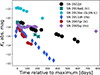 |
Fig. 22. Comparison of the MK between SN 2022jli and well observed core-collapse SNe in the NIR bands. |
The process of dust formation and the heating mechanism of the dust detected in SN 2022jli is not obvious, the dust may be newly formed in the ejecta or pre-existing dust in the CSM. The first scenario is emission from hot newly condensed dust in the SN ejecta or in a cool dense shell (CDS) produced by the interaction of the ejecta with a dense CSM shell. Alternatively pre-existing CSM dust may be radiatively heated by the SN luminosity, by the emission from the first and/or second maxima, producing dust thermal emission, denominated IR echo.
4. Discussion
A diverse set of mechanisms have been proposed to explain bumps and double-peaked light curves in SNe. Until recently, two main scenarios were usually invoked to explain double-peaked light curves. One is the power injection from a compact object such as a fast-spinning neutron star with a strong magnetic field (see e.g., Maeda et al. 2007) or fall-back accretion onto a compact object of stellar mass, such as a black hole or a neutron star. Alternatively, double-peaked light curves and bumps have been frequently considered smoking gun signatures of interaction with a dense CSM. In the following we analyse the potential scenarios to explain the strong bump displayed by SN 2022jli and its subsequent undulations.
4.1. Super-Eddington accretion
Recently, Chen et al. (2024) proposed that the second maximum and the subsequent periodic undulations observed in SN 2022jli are the result of the mass accretion from a companion star onto a compact object in a binary system at their periastron encounters. In this paper, the estimated (pseudo) bolometric luminosity of the second maximum is ∼1.7 × 1042 erg s−111, this corresponds to ∼103 and ∼104 times the Eddington ratio (REdd) for a black-hole mass (Mbh) of 10 M⊙ and a neutron star mass (Mns) of 1.4 M⊙, respectively.
Super-Eddington accretion into a compact object has been considered as the most likely possibility to explain ultra-luminous X-rays sources (ULXs; see Kaaret et al. 2017, for a review), such as NGC 5907 ULX (Israel et al. 2017). These sources can reach X-ray luminosities in excess of a few 1039 erg s−1, which is the Eddington luminosity (LEdd) for a 10 M⊙ black hole. NGC 5907 ULX is one of the brightest examples of this class, reaching a luminosity of ∼2 × 1041 erg s−1, and it might harbour a binary system composed of a neutron star accreting at ∼103 times the LEdd from the companion star, assuming isotropic luminosity (Israel et al. 2017). However, significant collimation of the disc radiation and strong multi-polar magnetic fields are required to explain the extreme luminosity of NGC 5907 ULX (Israel et al. 2017). In the presence of a strong magnetic field (> 1013 G) the electron scattering cross sections in the extraordinary mode are reduced for photon energies below the cyclotron energy ( keV; Herold 1979); thus, radiation can escape without halting the accretion flow (Israel et al. 2017). The assumption of isotropic emission in ULXs strongly overestimates the total radiation output. For example Cygnus X-3 in our galaxy, seems to be an ULX viewed side-on suffering significant geometrical beaming (Veledina et al. 2024).
Chen et al. (2024) reported the detection of an Hα feature showing a shift in the peak emission and where its luminosity follows the periodic undulations of the light curve of SN 2022jli. This variability in the Hα feature would be the result of the accretion of hydrogen-rich material from a companion star at periastron encounters as was discussed previously. Chen et al. (2024) also report a non-detection of the SN in X-rays placing an upper limit of 2.5 × 1040 erg s−1 in the 30 − 60 keV energy range at about +230 days from NuSTAR observations, and of 1.32 × 1038 erg s−1 in the 0.5 − 7 keV energy range at about +260 days from Chandra observations.
The soft X-ray (0.5 − 2 keV) opacity of CC SNe can remain very large for decades, even in SE SNe that are expected to have a factor of 10 lower opacities compared to Type II SNe due to their faster ejecta (Alp et al. 2018). Assuming that the opacity of SN 2022jli is similar to the SN IIb models of Alp et al. (2018), we estimate that at the time of the X-ray observations the opacity at 2 keV, 10 keV, and 50 keV are ∼304, 103, and 40, respectively. Thus all the potential X-ray emission from a central source is absorbed and reprocessed by the SN ejecta, note that the ejecta opacity is larger for the soft X-rays than for more energetic emission. The reprocessing scenario is consistent with the blue optical SN colours, the increase in the ejecta temperature during the re-brightening12, and the unusual detection of Mg II lines in the NIR at more than 150 days, implying that the SN emission in the optical and in the NIR bands is from a heated SN ejecta and not direct emission from a central source. At later times (< 350 days), the ejecta becomes fully nebular showing strong [O I] lines (Fig. 14).
Following the Chen et al. (2024) hypothesis, King & Lasota (2024) proposed an scenario in which the second maximum of SN 2022jli is produced by a highly beamed ULX, with a beaming factor of b ∼ 10−3 or b ∼ 10−4 for a 10 M⊙ black hole or a neutron star, respectively. Additionally, King & Lasota (2024) propose that the second maximum corresponds to an ultra-soft ULX emitting mostly in the UVOIR region of the electromagnetic spectrum. They propose that the orbital plane must be misaligned with respect to the axis of the beamed emission to detect the highly beamed ULX emission and simultaneously observe the shift in the Hα emission produced by the orbital motion and accretion from the (low-mass) companion star. The fact that the emission during the second maximum seems to correspond to emission from heated ejecta and not to direct UVOIR emission from an ultra-soft ULX, in addition to the extreme beaming required to explain the high luminosity of SN 2022jli, and the fine tuned geometry to detect both the highly beamed emission from the ULX and the Hα periodic variability cast some doubts on the feasibility of the scenario proposed by King & Lasota (2024).
Recent hydrodynamical simulations of (Hirai et al. 2025) show that the luminosity and the undulations of SN 2022jli can be reproduced by the accretion from a shock-inflated companion star into a neutron star. The model of (Hirai et al. 2025) also predicts a temperature increase (blue colours) at periastron encounters (higher luminosity), as is discussed in Section 3.2.5, but not the increase in the ejecta temperature observed in Fig. 13. Similarly, (Lu et al. 2025) presented an analytical model for the super-Eddington accretion from a shock-inflated companion star that reproduces the main characteristics of the bolometric light curve. This model predicts that, in addition to the hydrogen-rich material accreted into the neutron star, a significant amount of material from the companion star is ejected (∼10−3 − 10−2 M⊙; Hirai et al. 2025; Lu et al. 2025) at a velocity of a few ×103 km s−1 (Lu et al. 2025). In principle, the detection of emission lines from the ejected material at the nebular phase could be a smoking gun signature of this model. Such hydrogen-rich material is not detected in our nebular phase spectra, which requires further modelling and investigation.
4.2. Power injection from a magnetar
Neutron stars are one possible outcome of core-collapse SNe, and usually possess strong magnetic fields. Magnetars are a type of neutron star and possess strong magnetic fields in the range of 1013 − 1015 G. The physics associated with the formation of magnetars is poorly understood. The magnetars in our galaxy exhibit the most variable behaviour among neutron stars, emitting high energy electromagnetic radiation mostly in the hard X-rays and soft γ-rays (LX ∼ 5 × 1030 − 1036 erg s−1; Kaspi & Beloborodov 2017), and are faint at optical wavelengths. If a fast-spinning neutron star with a strong magnetic field is formed, the rotational spin-down energy of the magnetar can contribute to power the SN light curve. However, the energy injection and the ejecta thermalisation process of the magnetar wind are a complex phenomena (see e.g., Kotera et al. 2013; Vurm & Metzger 2021) that can vary with time, producing humps, bumps, or even periodic undulations in the SN light curves (Vurm & Metzger 2021; Moriya et al. 2022).
Since the discovery of the double-peaked SN 2005bf, the power injection from a magnetar has been recognised as a viable mechanism to produce double-peaked light curves (Maeda et al. 2007). As is discussed in Israel et al. (2017), the magnetic field configuration required for the neutron star in NGC 5907 ULX to accrete at a super-Eddington rate is similar to the one envisaged for the so-called magnetars, and as was discussed in Medvedev & Poutanen (2013), young pulsars or magnetars can be potential ULXs. Therefore, a natural possibility is that the compact object in SN 2022jli is a magnetar accreting material from a companion star. This is similar to the scenario proposed by Chen et al. (2024), but where a significant fraction of the power supply could come from the magnetar, avoiding the need for super-Eddington accretion to power the second maximum or a privileged viewing angle to an extremely beamed ULX. In this scenario, the accretion at periastron encounters could explain the undulations and the Hα periodic variability.
Moriya et al. (2022) studied the effect of variable thermal energy injection in the SN ejecta from a magnetar as the potential cause of bumps in SN light curves. They found that changes in the thermal power injection produced in the SN ejecta from a magnetar can reproduce the light curve bumps such as the ones observed in some SLSNe (e.g., SN 2015bn). One of Moriya et al. (2022) predictions is that an observable consequence of the increase in the power input from a magnetar is an increase in the SN ejecta temperature, in addition to the luminosity increase. The temperature increase should translate in bluer SN colours during the bump, such as the bluer g − r colours observed in SN 2022jli during the maxima of the second bump and the undulations (see Figs. 9 and 10). Their model also predicts a non-noticeable change in the ejecta radius or velocity during the luminosity increase. The latter effect seems to discount a magnetar power supply to explain, for example, the second maximum in the case of SN 2019stc (Moriya et al. 2022).
Potential causes of the change in the thermal energy injection are: i) conversion efficiency, inefficient thermalisation at early times (e.g., Kasen et al. 2016), ii) changes in the fraction of high-energy photons in the pulsar wind nebulae can lead to a change in the thermalisation of the energy injected, since the opacity depends on the energy of the photons injected, iii) a change in the angle between the dipole magnetic field and the rotation axis of the neutron star changes the temporal energy injection, and iv) fallback accretion on the magnetar can increase the mass and the angular momentum of the neutron star, decreasing the magnetar spin period. A periodic variation in the angle between the magnetic field axis and the rotation axis of the magnetar should yield periodic variability in the light curves. However, this cannot explain the periodic variation observed in the H I lines.
To explore the magnetar scenario, it is assumed that the second maximum is powered by a magnetar. As is discussed in Section 3.2.8, the first maximum of SN 2022jli is consistent with a standard SE SN event with an ejecta mass of about 1.5 M⊙. Following a methodology similar to the one described in Cartier et al. (2022), and assuming the same ejecta parameters used to fit the first maximum (Section 3.2.8), the second maximum of SN 2022jli is reproduced by the combination of the radioactive decay of 0.12 M⊙ of 56Ni and the power input from a magnetar (see Fig. 13). We assume full trapping over the period analysed (no power leakage), with κ = 0.07 cm2 gr−1 and vej = 8500 km s−1, obtaining an initial spin period of P ∼ 48.5 ms and a magnetic field of B ∼ 8.5 × 10¹⁴ G. We had to arbitrarily delay the “birth” of the magnetar by 37 days relative to the estimated time of the explosion to reproduce the (pseudo) bolometric light curve of SN 2022jli. In this scenario the late time γ-ray emission reported by Chen et al. (2024) could be interpreted as the emergence of a magnetar wind nebulae (see e.g., Kotera et al. 2013), bringing as a result a drop in the light curve due to leakage of the magnetar power supply. The drop below the luminosity of the radioactive decay chain of 0.12 M⊙ of 56Ni at +383 requires the escape of a significant amount of γ-rays from the radioactive decay of 56Co. The assumption of full trapping and fixed opacity are probably not realistic, but our modelling provides evidence that the secondary maximum could be at least partially, if not completely, powered by a magnetar.
Recently, (Orellana et al. 2025) presented a hydrodynamic modelling of the bolometric light curve of SN 2022jli of Chen et al. (2024). They obtain a good fit of the double-peaked light curve using a hybrid model that combines the radioactive decay of 56Ni and a magnetar. Assuming that magnetar power ceases to be efficiently thermalised at ∼270 days, they reproduce the rapid light curve drop. This model does not produce the small periodic undulations of SN 2022jli that may arise from the interaction between a neutron star and a companion star in a binary system. Orellana et al. (2025) obtain a similar 56Ni mass to our analytical model, and consistent parameters for the magnetic field and the spin of the magnetar The main difference is in the ejecta mass, where they obtain Mej = 9.55 M⊙. This significant difference may arise from the limitations of our simple analytical model, in addition to the differences between our pseudo-bolometric light curve and that of Chen et al. (2024).
4.3. Ejecta circumstellar interaction
The interaction between the SN ejecta and a dense CSM can efficiently transform the kinetic energy of the SN ejecta in thermal energy, powering the SN brightness. This is mechanism behind interacting SLSNe-IIn such as SN 2006gy (Smith et al. 2007), and it has been proposed to explain the large maximum luminosities of SLSNe-Ic (Sorokina et al. 2016; Tolstov et al. 2017a,b). There is evidence that the SN ejecta-CSM interaction may be responsible for the bumps or the light curve undulations observed in some SLSNe after maximum light (Yan et al. 2015, 2017). Some SE SNe such as SN 2014C (Milisavljevic et al. 2015), SN 2017ens (Chen et al. 2018), SN 2017dio (Kuncarayakti et al. 2018), and SN 2018ijp (Tartaglia et al. 2021) interact with abundant hydrogen-rich CSM, becoming Type IIn SNe. In fact, the presence of dense CSM is a natural consequence of the stellar stripping and bumps in the light curves are often considered a signature of the ejecta-CSM interaction.
As is discussed in Chen et al. (2024), it is unlikely that the undulations and the light curve of SN 2022jli is powered by ejecta-CSM interaction because the interaction on the rear side would smear any periodic signature from the near side. Additionally, we consider that the spectroscopic evolution of SN 2022jli lack clear signatures of ejecta-CSM interaction.
The evolution of Rbb can provide insights into the power mechanism. The radiative shock produced by the interaction propagates throughout the dense CSM increasing the optical depth and as a consequence the photospheric radius at the same time (Moriya et al. 2018). Such an increase in Rbb has been observed in the double-peaked superluminous SN2019stc (Gomez et al. 2021; Moriya et al. 2022) and in the double-peaked luminous type II ASASSN-13dn (Hueichapán et al. 2025b), for example. Both SNe are double-peaked but show no clear signs of interaction such as narrow CSM emission features. The Rbb evolution in interacting type IIn SNe is diverse, but generally show an increase at early times, in particular before maximum light, a flat evolution or a slow decrease in their Rbb after maximum (see e.g., Taddia et al. 2013; Ofek et al. 2014). A very rapid increase in Rbb in type IIn SNe has been also reported, which has been interpreted as a signature of aspherical CSM (see Soumagnac et al. 2019, 2020). On the other hand, SN 2022jli shows the opposite, a decrease in Rbb during the SN re-brightening (see Fig. 12). The second maximum of SN 2022jli is produced by an energy source that heats the ejecta, this is manifested by the increase in the temperature, but not in the radius. Thus we consider the ejecta-CSM interaction an unlikely scenario to explain the second maximum of SN 2022jli.
5. Summary
We have presented and analysed observations of the SE SN 2022jli, which exhibits a double-peaked light curve with two maxima separated by about 50 days. After the second maximum, the well-sampled ZTF and ATLAS light curves reveal periodic undulations with a period of about 12.5 days (see also Moore et al. 2023; Chen et al. 2024). Using synthetic photometry inferred from spectra obtained during the decline from the first maximum, a host galaxy reddening of E(B − V)host = 0.23 ± 0.06 was estimated. The SN shows unusually blue g − r colours during its re-brightening, reaching its bluest colour (g − r ≃ −0.45 mag) at +190 days relative to maximum. We found that in addition to the blue colours the SN shows clear colour variations during its periodic undulations, becoming blue when brighter and redder when becomes fainter, showing more conspicuous periodic undulations in the bluer bands.
The first maximum of SN 2022jli is consistent with a SN Ic with an estimated expansion velocity of 8500 km s−1, an ejecta mass of ∼1.5 M⊙, and a radioactive 56Ni mass of ∼0.12 M⊙ (see also Orellana et al. 2025). The available photometry seems to show a smooth evolution and does not show undulations during the first maximum, although this cannot be completely discounted due to the sparse coverage in terms of wavelength and sampling of the first maximum. The late optical spectra (> + 400 days) confirm the SN Ic nature of SN 2022jli.
We report the detection of relatively weak and broad Hα and Paβ double-peaked spectral features. The main peak of Hα and Paβ features seems to shift following the periodic variation of the light curve undulations, as has been reported by Chen et al. (2024) for Hα. We notice that these features become more conspicuous with time, particularly after +100 days. The shift in the H I spectral features is probably a signature of the accretion of hydrogen-rich material from a companion star in a binary system. When the spectra of the SN become nebular (> + 350 days), the hydrogen signatures are not longer detectable in the optical or in the NIR spectra; however, narrow unresolved Hα emission most likely from the host galaxy is detected at late times (FWHM < 400 km s−1).
The second maximum was reproduced using the analytical solutions of Arnett (1982) with a hybrid model that combines the radioactive decay of 0.12 M⊙ of 56Ni and the power injection from a magnetar with P ∼ 48 ms and B ∼ 8 × 10¹⁴ G. During the revision of this article, a similar hydrodynamical model of the bolometric luminosity of SN 2022jli was presented by Orellana et al. (2025). This demonstrates that the double-peaked light curve of SN 2022jli could be powered by a hybrid model that includes a magnetar. In this scenario, the magnetar contributes to the second maximum, and moderate accretion from a companion star is necessary to produce the small light curve undulations and the weak hydrogen lines observed after the second maximum. The power injection from a magnetar seems a viable scenario, since magnetars are the most variable neutron stars displaying different types of episodic variability (see Mereghetti et al. 2015; Kaspi & Beloborodov 2017). The magnetar contributing to power the second maximum of SN 2022jli could fit into the more general picture whereby magnetars are the power source of SLSNe-Ic and could produce their frequent bumps and undulations, and whereby pulsars could produce the late time excess observed in some SE SNe (see e.g., Taddia et al. 2016; Ravi et al. 2023). The possibility of a magnetar as an additional power source is not limited to ‘exotic’ SE SNe. Rodríguez et al. (2024) analysed 54 SNe IIb/Ib/Ic and found evidence of a central engine in most of them. If these engines are magnetars, then their initial magnetic fields and rotation periods align well with those expected for magnetars at birth.
Alternatively, the second maximum could be produced by the significant accretion of material from the companion star into the compact object left from the explosion (a black hole or a neutron star), at an extremely large super-Eddington accretion rate (∼103 for a black hole or ∼104 for a neutron star), or could be a ULX displaying extremely beamed emission (b ∼ 10−3 or 10−4) viewed just at the right angle, as has been proposed by King & Lasota (2024). A somewhat different scenario is the accretion from a shock-inflated companion star into the neutron star. This model seems to reproduce the bolometric luminosity (Hirai et al. 2025; Lu et al. 2025) and the undulations of SN 2022jli (Hirai et al. 2025), and predicts a significant mass ejection of hydrogen-rich material from the inflated envelope of the companion star (∼10−3 − 10−2 M⊙; Hirai et al. 2025; Lu et al. 2025). It is not clear whether this ejected material should be detectable in the nebular phase or not. This is an interesting model that requires further comparison with observations.
From +190 days until about +224 days, unambiguous first CO overtone emission is detected in the NIR spectra of SN 2022jli. At later times (> + 385 days), the first CO overtone is not longer detected. From about +200 days, a strong IR excess is detected in the NIR photometry of SN 2022jli, which is particularly strong in the Ks band. Later NIR observations (> + 385 days) demonstrate that this IR excess is produced by thermal emission from hot dust, with a temperature of 900–650 K. Depending on the assumptions of the dust composition, the estimated dust mass is 2 − 16 × 10−4 M⊙. This emission could be produced either by a strong IR echo from pre-existing dust surrounding the SN, or by newly formed dust in the SN ejecta. The detection of CO and of dust potentially formed in the ejecta of SN 2022jli is important for understanding the formation of molecules and dust formation in the ejecta of SE SNe. Future IR observations with JWST should complement the observations presented here, providing an unprecedented view of the molecule and dust emission in SN 2022jli over several years, or even over a decade-long timescale.
Data availability
The spectra are available on request to the corresponding author and also available from the WISeREP13 archive (Yaron & Gal-Yam 2012).
Acknowledgments
We thank to Ósmar Rodríguez and the anonymous referee for useful comments that helped to improve this manuscript. R.C. acknowledges support from Gemini ANID ASTRO21-0036. M.D.S. is funded by the Independent Research Fund Denmark (IRFD, grant number 10.46540/2032-00022B). J.L.P and M.G. acknowledges support from ANID, Millennium Science Initiative, AIM23-0001. R.C. thanks Maria Elisa Ugarte for her support. Based on observations obtained at the international Gemini Observatory under proposals GS-2022A-Q-415, GS-2022B-Q-407 and GS-2022B-FT-206 (PI R. Cartier), a program of NSF’s NOIRLab, which is managed by the Association of Universities for Research in Astronomy (AURA) under a cooperative agreement with the National Science Foundation on behalf of the Gemini Observatory partnership: the National Science Foundation (United States), National Research Council (Canada), Agencia Nacional de Investigación y Desarrollo (Chile), Ministerio de Ciencia, Tecnología e Innovación (Argentina), Ministério da Ciência, Tecnologia, Inovações e Comunicações (Brazil), and Korea Astronomy and Space Science Institute (Republic of Korea). Also based on observations obtained at the Southern Astrophysical Research (SOAR) telescope, which is a joint project of the Ministério da Ciência, Tecnologia e Inovações (MCTI/LNA) do Brasil, the US National Science Foundation’s NOIRLab, the University of North Carolina at Chapel Hill (UNC), and Michigan State University (MSU). Based on observations collected at the European Southern Observatory under ESO programmes 382.B-0331(A) and 108.220C.014. This research has made use of the NASA/IPAC Extragalactic Database (NED), which is operated by the Jet Propulsion Laboratory, California Institute of Technology, under contract with the National Aeronautics and Space Administration. This work has also made use of data from the Asteroid Terrestrial-impact Last Alert System (ATLAS) project. The Asteroid Terrestrial-impact Last Alert System (ATLAS) project is primarily funded to search for near earth asteroids through NASA grants NN12AR55G, 80NSSC18K0284, and 80NSSC18K1575; byproducts of the NEO search include images and catalogs from the survey area. This work was partially funded by Kepler/K2 grant J1944/80NSSC19K0112 and HST GO-15889, and STFC grants ST/T000198/1 and ST/S006109/1. The ATLAS science products have been made possible through the contributions of the University of Hawaii Institute for Astronomy, the Queen’s University Belfast, the Space Telescope Science Institute, the South African Astronomical Observatory, and The Millennium Institute of Astrophysics (MAS), Chile. This publication makes use of data products from the Wide-field Infrared Survey Explorer, which is a joint project of the University of California, Los Angeles, and the Jet Propulsion Laboratory/California Institute of Technology, funded by the National Aeronautics and Space Administration. This work has made use of data from the European Space Agency (ESA) mission Gaia (https://www.cosmos.esa.int/gaia), processed by the Gaia Data Processing and Analysis Consortium (DPAC, https://www.cosmos.esa.int/web/gaia/dpac/consortium). Funding for the DPAC has been provided by national institutions, in particular the institutions participating in the Gaia Multilateral Agreement.
References
- Afsariardchi, N., Drout, M. R., Khatami, D. K., et al. 2021, ApJ, 918, 89 [NASA ADS] [CrossRef] [Google Scholar]
- Alp, D., Larsson, J., Fransson, C., et al. 2018, ApJ, 864, 175 [Google Scholar]
- Anderson, J. P. 2019, A&A, 628, A7 [NASA ADS] [CrossRef] [EDP Sciences] [Google Scholar]
- Angus, C. R., Smith, M., Sullivan, M., et al. 2019, MNRAS, 487, 2215 [NASA ADS] [CrossRef] [Google Scholar]
- Anupama, G. C., Sahu, D. K., Deng, J., et al. 2005, ApJ, 631, L125 [NASA ADS] [CrossRef] [Google Scholar]
- Arnett, W. D. 1982, ApJ, 253, 785 [Google Scholar]
- Balcon, C. 2022, Transient Name Server Classification Report, 2022–3048, 1 [Google Scholar]
- Banerjee, D. P. K., Joshi, V., Evans, A., et al. 2018, MNRAS, 481, 806 [CrossRef] [Google Scholar]
- Becker, A. 2015, Astrophysics Source Code Library [record ascl:1504.004] [Google Scholar]
- Bellm, E. C., Kulkarni, S. R., Graham, M. J., et al. 2019, PASP, 131, 018002 [Google Scholar]
- Bersten, M. C., Benvenuto, O., & Hamuy, M. 2011, ApJ, 729, 61 [NASA ADS] [CrossRef] [Google Scholar]
- Bersten, M. C., Benvenuto, O. G., Nomoto, K., et al. 2012, ApJ, 757, 31 [Google Scholar]
- Bouchet, P., Phillips, M. M., Suntzeff, N. B., et al. 1991, A&A, 245, 490 [NASA ADS] [Google Scholar]
- Buzzoni, B., Delabre, B., Dekker, H., et al. 1984, The Messenger, 38, 9 [NASA ADS] [Google Scholar]
- Cano, Z. 2013, MNRAS, 434, 1098 [Google Scholar]
- Cartier, R., Rho, J., Hoeflich, P., et al. 2021, ATel, 14653, 1 [Google Scholar]
- Cartier, R., Hamuy, M., Contreras, C., et al. 2022, MNRAS, 514, 2627 [NASA ADS] [CrossRef] [Google Scholar]
- Catchpole, R. M., Whitelock, P. A., Feast, M. W., et al. 1988, MNRAS, 231, 75P [NASA ADS] [CrossRef] [Google Scholar]
- Chatzopoulos, E., Wheeler, J. C., Vinko, J., Horvath, Z. L., & Nagy, A. 2013, ApJ, 773, 76 [NASA ADS] [CrossRef] [Google Scholar]
- Chen, P., Gal-Yam, A., Sollerman, J., et al. 2024, Nature, 625, 253 [NASA ADS] [CrossRef] [Google Scholar]
- Chen, T. W., Inserra, C., Fraser, M., et al. 2018, ApJ, 867, L31 [NASA ADS] [CrossRef] [Google Scholar]
- Clemens, J. C., Crain, J. A., & Anderson, R. 2004, SPIE Conf. Ser., 5492, 331 [NASA ADS] [Google Scholar]
- Conti, P. S. 1975, Memoires of the Societe Royale des Sciences de Liege, 9, 193 [Google Scholar]
- Cosentino, S. P., Evans, C. R., Inserra, C., et al. 2022, Transient Name Server Classification Report, 2022–1409, 1 [Google Scholar]
- Cushing, M. C., Vacca, W. D., & Rayner, J. T. 2004, PASP, 116, 362 [NASA ADS] [CrossRef] [Google Scholar]
- Dalton, G. B., Caldwell, M., Ward, A. K., et al. 2006, SPIE Conf. Ser., 6269, 62690X [Google Scholar]
- De Cia, A., Gal-Yam, A., Rubin, A., et al. 2018, ApJ, 860, 100 [NASA ADS] [CrossRef] [Google Scholar]
- Dessart, L., Hillier, D. J., Woosley, S., et al. 2015, MNRAS, 453, 2189 [NASA ADS] [CrossRef] [Google Scholar]
- Dessart, L., Yoon, S.-C., Aguilera-Dena, D. R., & Langer, N. 2020, A&A, 642, A106 [NASA ADS] [CrossRef] [EDP Sciences] [Google Scholar]
- Dessart, L., Kotak, R., Jacobson-Galán, W., et al. 2025, A&A, 704, L6 [NASA ADS] [CrossRef] [EDP Sciences] [Google Scholar]
- Dong, Y., Valenti, S., Ashall, C., et al. 2024, ApJ, 974, 316 [NASA ADS] [CrossRef] [Google Scholar]
- Draine, B. T. 2016, ApJ, 831, 109 [NASA ADS] [CrossRef] [Google Scholar]
- Draine, B. T., & Lee, H. M. 1984, ApJ, 285, 89 [NASA ADS] [CrossRef] [Google Scholar]
- Drout, M. R., Soderberg, A. M., Gal-Yam, A., et al. 2011, ApJ, 741, 97 [NASA ADS] [CrossRef] [Google Scholar]
- Drout, M. R., Milisavljevic, D., Parrent, J., et al. 2016, ApJ, 821, 57 [NASA ADS] [CrossRef] [Google Scholar]
- Eikenberry, S., Bandyopadhyay, R., Bennett, J. G., et al. 2012, Proc. SPIE, 8446, 84460I [Google Scholar]
- Eikenberry, S. S., Elston, R., Raines, S. N., et al. 2004, Proc. SPIE, 5492, 1196 [Google Scholar]
- Elias, J. H., Gregory, B., Phillips, M. M., et al. 1988, ApJ, 331, L9 [Google Scholar]
- Emerson, J., McPherson, A., & Sutherland, W. 2006, The Messenger, 126, 41 [NASA ADS] [Google Scholar]
- Ergon, M., Jerkstrand, A., Sollerman, J., et al. 2015, A&A, 580, A142 [NASA ADS] [CrossRef] [EDP Sciences] [Google Scholar]
- Ergon, M., Sollerman, J., Fraser, M., et al. 2014, A&A, 562, A17 [NASA ADS] [CrossRef] [EDP Sciences] [Google Scholar]
- Fang, Q., Maeda, K., Kuncarayakti, H., et al. 2022, ApJ, 928, 151 [NASA ADS] [CrossRef] [Google Scholar]
- Filippenko, A. V. 1997, ARA&A, 35, 309 [NASA ADS] [CrossRef] [Google Scholar]
- Fitzpatrick, E. L. 1999, PASP, 111, 63 [Google Scholar]
- Folatelli, G., Contreras, C., Phillips, M. M., et al. 2006, ApJ, 641, 1039 [NASA ADS] [CrossRef] [Google Scholar]
- Gaia Collaboration (Prusti, T., et al.) 2016, A&A, 595, A1 [NASA ADS] [CrossRef] [EDP Sciences] [Google Scholar]
- Gal-Yam, A. 2017, in Handbook of Supernovae, eds. A. W. Alsabti, & P. Murdin, 195 [Google Scholar]
- Gerardy, C. L., Fesen, R. A., Nomoto, K., et al. 2002, PASJ, 54, 905 [NASA ADS] [CrossRef] [Google Scholar]
- Gimeno, G., Roth, K., Chiboucas, K., et al. 2016, SPIE Conf. Ser., 9908, 99082S [NASA ADS] [Google Scholar]
- Gomez, S., Berger, E., Hosseinzadeh, G., et al. 2021, ApJ, 913, 143 [NASA ADS] [CrossRef] [Google Scholar]
- González-Gaitán, S., Gutiérrez, C. P., Anderson, J. P., et al. 2024, A&A, 687, A108 [NASA ADS] [CrossRef] [EDP Sciences] [Google Scholar]
- Grzegorzek, J. 2022, Transient Name Server Classification Report, 2022–1261, 1 [Google Scholar]
- Gutiérrez, C. P., Bersten, M. C., Orellana, M., et al. 2021, MNRAS, 504, 4907 [CrossRef] [Google Scholar]
- Gutiérrez, C. P., Pastorello, A., Bersten, M., et al. 2022, MNRAS, 517, 2056 [CrossRef] [Google Scholar]
- Hamuy, M., Folatelli, G., Morrell, N. I., et al. 2006, PASP, 118, 2 [NASA ADS] [CrossRef] [Google Scholar]
- Herold, H. 1979, Phys. Rev. D, 19, 2868 [NASA ADS] [CrossRef] [Google Scholar]
- Hirai, R., & Podsiadlowski, P. 2022, MNRAS, 517, 4544 [Google Scholar]
- Hirai, R., Podsiadlowski, P., Hoeflich, P., et al. 2025, ApJ, 995, 55 [Google Scholar]
- Holmbo, S., Stritzinger, M. D., Karamehmetoglu, E., et al. 2023, A&A, 675, A83 [NASA ADS] [CrossRef] [EDP Sciences] [Google Scholar]
- Hook, I. M., Jørgensen, I., Allington-Smith, J. R., et al. 2004, PASP, 116, 425 [NASA ADS] [CrossRef] [Google Scholar]
- Hosseinzadeh, G., Berger, E., Metzger, B. D., et al. 2022, ApJ, 933, 14 [NASA ADS] [CrossRef] [Google Scholar]
- Hueichapán, E., Cartier, R., Prieto, J. L., et al. 2025a, ArXiv e-prints [arXiv:2508.02656] [Google Scholar]
- Hueichapán, E., Prieto, J. L., Cartier, R., et al. 2025b, A&A, 702, A47 [NASA ADS] [CrossRef] [EDP Sciences] [Google Scholar]
- Hueichapan, E. D., Contreras, C., Cartier, R., et al. 2022, MNRAS, 513, 2965 [Google Scholar]
- Hunter, D. J., Valenti, S., Kotak, R., et al. 2009, A&A, 508, 371 [NASA ADS] [CrossRef] [EDP Sciences] [Google Scholar]
- Inserra, C., Smartt, S. J., Jerkstrand, A., et al. 2013, ApJ, 770, 128 [NASA ADS] [CrossRef] [Google Scholar]
- Israel, G. L., Belfiore, A., Stella, L., et al. 2017, Science, 355, 817 [NASA ADS] [CrossRef] [Google Scholar]
- Itagaki, K. 2022, Transient Name Server Discovery Report, 2022–3014, 1 [Google Scholar]
- Jacobson-Galán, W. V., Dessart, L., Kilpatrick, C. D., et al. 2025, ApJ, 994, L14 [Google Scholar]
- Kaaret, P., Feng, H., & Roberts, T. P. 2017, ARA&A, 55, 303 [Google Scholar]
- Kasen, D. 2010, ApJ, 708, 1025 [Google Scholar]
- Kasen, D., & Bildsten, L. 2010, ApJ, 717, 245 [NASA ADS] [CrossRef] [Google Scholar]
- Kasen, D., Metzger, B. D., & Bildsten, L. 2016, ApJ, 821, 36 [CrossRef] [Google Scholar]
- Kaspi, V. M., & Beloborodov, A. M. 2017, ARA&A, 55, 261 [Google Scholar]
- Khatami, D. K., & Kasen, D. N. 2019, ApJ, 878, 56 [NASA ADS] [CrossRef] [Google Scholar]
- King, A., & Lasota, J.-P. 2024, A&A, 682, L22 [NASA ADS] [CrossRef] [EDP Sciences] [Google Scholar]
- Kotak, R., Meikle, P., van Dyk, S. D., Höflich, P. A., & Mattila, S. 2005, ApJ, 628, L123 [Google Scholar]
- Kotak, R., Meikle, P., Pozzo, M., et al. 2006, ApJ, 651, L117 [Google Scholar]
- Kotak, R., Meikle, W. P. S., Farrah, D., et al. 2009, ApJ, 704, 306 [NASA ADS] [CrossRef] [Google Scholar]
- Kotera, K., Phinney, E. S., & Olinto, A. V. 2013, MNRAS, 432, 3228 [NASA ADS] [CrossRef] [Google Scholar]
- Krisciunas, K., Contreras, C., Burns, C. R., et al. 2017, AJ, 154, 211 [NASA ADS] [CrossRef] [Google Scholar]
- Kuncarayakti, H., Maeda, K., Ashall, C. J., et al. 2018, ApJ, 854, L14 [NASA ADS] [CrossRef] [Google Scholar]
- Kuncarayakti, H., Sollerman, J., Izzo, L., et al. 2023, A&A, 678, A209 [NASA ADS] [CrossRef] [EDP Sciences] [Google Scholar]
- Lang, D., Hogg, D. W., Mierle, K., Blanton, M., & Roweis, S. 2010, AJ, 139, 1782 [Google Scholar]
- Laor, A., & Draine, B. T. 1993, ApJ, 402, 441 [NASA ADS] [CrossRef] [Google Scholar]
- Leloudas, G., Chatzopoulos, E., Dilday, B., et al. 2012, A&A, 541, A129 [NASA ADS] [CrossRef] [EDP Sciences] [Google Scholar]
- Liljegren, S., Jerkstrand, A., & Grumer, J. 2020, A&A, 642, A135 [EDP Sciences] [Google Scholar]
- Lu, W., Cary, S., & Tsuna, D. 2025, ArXiv e-prints [arXiv:2507.14284] [Google Scholar]
- Lunnan, R., Chornock, R., Berger, E., et al. 2018, ApJ, 852, 81 [NASA ADS] [CrossRef] [Google Scholar]
- Lyman, J. D., Bersier, D., James, P. A., et al. 2016, MNRAS, 457, 328 [Google Scholar]
- Maeda, K., Tanaka, M., Nomoto, K., et al. 2007, ApJ, 666, 1069 [NASA ADS] [CrossRef] [Google Scholar]
- Maeda, K., Kawabata, K., Mazzali, P. A., et al. 2008, Science, 319, 1220 [NASA ADS] [CrossRef] [Google Scholar]
- Mainzer, A., Grav, T., Bauer, J., et al. 2011, ApJ, 743, 156 [NASA ADS] [CrossRef] [Google Scholar]
- Mainzer, A., Bauer, J., Cutri, R. M., et al. 2014, ApJ, 792, 30 [Google Scholar]
- Medler, K., Ashall, C., Shahbandeh, M., et al. 2025, ApJS, 281, 28 [Google Scholar]
- Medvedev, A. S., & Poutanen, J. 2013, MNRAS, 431, 2690 [Google Scholar]
- Meikle, W. P. S., Allen, D. A., Spyromilio, J., & Varani, G. F. 1989, MNRAS, 238, 193 [NASA ADS] [CrossRef] [Google Scholar]
- Mereghetti, S., Pons, J. A., & Melatos, A. 2015, Space Sci. Rev., 191, 315 [NASA ADS] [CrossRef] [Google Scholar]
- Milisavljevic, D., Margutti, R., Kamble, A., et al. 2015, ApJ, 815, 120 [NASA ADS] [CrossRef] [Google Scholar]
- Milne, P. A., The, L. S., & Leising, M. D. 1999, ApJS, 124, 503 [Google Scholar]
- Monard, L. 2022, Transient Name Server Discovery Report, 2022–1198, 1 [Google Scholar]
- Monard, L. A. G., Moore, M., & Li, W. 2005, IAU Circ., 8507, 1 [NASA ADS] [Google Scholar]
- Moore, T., Smartt, S. J., Nicholl, M., et al. 2023, ApJ, 956, L31 [NASA ADS] [CrossRef] [Google Scholar]
- Moriya, T. J., Sorokina, E. I., & Chevalier, R. A. 2018, Space Sci. Rev., 214, 59 [Google Scholar]
- Moriya, T. J., Murase, K., Kashiyama, K., & Blinnikov, S. I. 2022, MNRAS, 513, 6210 [NASA ADS] [CrossRef] [Google Scholar]
- Mould, J. R., Huchra, J. P., Freedman, W. L., et al. 2000, ApJ, 529, 786 [Google Scholar]
- Nicholl, M., Berger, E., Margutti, R., et al. 2016a, ApJ, 828, L18 [NASA ADS] [CrossRef] [Google Scholar]
- Nicholl, M., Berger, E., Smartt, S. J., et al. 2016b, ApJ, 826, 39 [NASA ADS] [CrossRef] [Google Scholar]
- Nicholl, M., & Smartt, S. J. 2016, MNRAS, 457, L79 [NASA ADS] [CrossRef] [Google Scholar]
- Nicholl, M., Smartt, S. J., Jerkstrand, A., et al. 2015, ApJ, 807, L18 [NASA ADS] [CrossRef] [Google Scholar]
- Ofek, E. O., Zoglauer, A., Boggs, S. E., et al. 2014, ApJ, 781, 42 [CrossRef] [Google Scholar]
- Orellana, M., & Bersten, M. C. 2022, A&A, 667, A92 [NASA ADS] [CrossRef] [EDP Sciences] [Google Scholar]
- Orellana, M., Bersten, M. C., & Gutiérrez, C. P. 2025, A&A, 700, L17 [NASA ADS] [CrossRef] [EDP Sciences] [Google Scholar]
- Park, S. H., Rho, J., Yoon, S.-C., et al. 2025, A&A, 703, A227 [NASA ADS] [CrossRef] [EDP Sciences] [Google Scholar]
- Phillips, M. M., Simon, J. D., Morrell, N., et al. 2013, ApJ, 779, 38 [NASA ADS] [CrossRef] [Google Scholar]
- Piro, A. L. 2015, ApJ, 808, L51 [NASA ADS] [CrossRef] [Google Scholar]
- Piro, A. L., Haynie, A., & Yao, Y. 2021, ApJ, 909, 209 [NASA ADS] [CrossRef] [Google Scholar]
- Podsiadlowski, P., Joss, P. C., & Hsu, J. J. L. 1992, ApJ, 391, 246 [Google Scholar]
- Poznanski, D., Prochaska, J. X., & Bloom, J. S. 2012, MNRAS, 426, 1465 [Google Scholar]
- Prentice, S. J., Mazzali, P. A., Pian, E., et al. 2016, MNRAS, 458, 2973 [NASA ADS] [CrossRef] [Google Scholar]
- Prentice, S. J., Maguire, K., Siebenaler, L., & Jerkstrand, A. 2022, MNRAS, 514, 5686 [NASA ADS] [CrossRef] [Google Scholar]
- Ravi, A. P., Rho, J., Park, S., et al. 2023, ApJ, 950, 14 [CrossRef] [Google Scholar]
- Rho, J., Geballe, T. R., Banerjee, D. P. K., et al. 2018, ApJ, 864, L20 [Google Scholar]
- Rho, J., Evans, A., Geballe, T. R., et al. 2021, ApJ, 908, 232 [NASA ADS] [CrossRef] [Google Scholar]
- Richmond, M. W., Treffers, R. R., Filippenko, A. V., et al. 1994, AJ, 107, 1022 [Google Scholar]
- Rodríguez, Ó., Maoz, D., & Nakar, E. 2023, ApJ, 955, 71 [CrossRef] [Google Scholar]
- Rodríguez, Ó., Nakar, E., & Maoz, D. 2024, Nature, 628, 733 [Google Scholar]
- Ryder, S. D., Zasov, A. V., McIntyre, V. J., Walsh, W., & Sil’chenko, O. K. 1998, MNRAS, 293, 411 [Google Scholar]
- Sana, H., de Mink, S. E., de Koter, A., et al. 2012, Science, 337, 444 [Google Scholar]
- Schlafly, E. F., & Finkbeiner, D. P. 2011, ApJ, 737, 103 [Google Scholar]
- Schlawin, E., Herter, T. L., Henderson, C., et al. 2014, SPIE Conf. Ser., 9147, 91472H [NASA ADS] [Google Scholar]
- Schlegel, D. J., Finkbeiner, D. P., & Davis, M. 1998, ApJ, 500, 525 [Google Scholar]
- Shahbandeh, M., Hsiao, E. Y., Ashall, C., et al. 2022, ApJ, 925, 175 [NASA ADS] [CrossRef] [Google Scholar]
- Shahbandeh, M., Sarangi, A., Temim, T., et al. 2023, MNRAS, 523, 6048 [NASA ADS] [CrossRef] [Google Scholar]
- Shappee, B. J., Prieto, J. L., Grupe, D., et al. 2014, ApJ, 788, 48 [Google Scholar]
- Sharon, A., & Kushnir, D. 2020, MNRAS, 496, 4517 [CrossRef] [Google Scholar]
- Shivvers, I., Filippenko, A. V., Silverman, J. M., et al. 2019, MNRAS, 482, 1545 [Google Scholar]
- Smartt, S. J., Valenti, S., Fraser, M., et al. 2015, A&A, 579, A40 [NASA ADS] [CrossRef] [EDP Sciences] [Google Scholar]
- Smith, K. W., Smartt, S. J., Young, D. R., et al. 2020, PASP, 132, 085002 [Google Scholar]
- Smith, M., Sullivan, M., D’Andrea, C. B., et al. 2016, ApJ, 818, L8 [NASA ADS] [CrossRef] [Google Scholar]
- Smith, N., Li, W., Foley, R. J., et al. 2007, ApJ, 666, 1116 [NASA ADS] [CrossRef] [Google Scholar]
- Snodgrass, C., Saviane, I., Monaco, L., & Sinclaire, P. 2008, The Messenger, 132, 18 [NASA ADS] [Google Scholar]
- Sorokina, E., Blinnikov, S., Nomoto, K., Quimby, R., & Tolstov, A. 2016, ApJ, 829, 17 [NASA ADS] [CrossRef] [Google Scholar]
- Soumagnac, M. T., Ofek, E. O., Gal-yam, A., et al. 2019, ApJ, 872, 141 [NASA ADS] [CrossRef] [Google Scholar]
- Soumagnac, M. T., Ofek, E. O., Liang, J., et al. 2020, ApJ, 899, 51 [Google Scholar]
- Springob, C. M., Haynes, M. P., Giovanelli, R., & Kent, B. R. 2005, ApJS, 160, 149 [NASA ADS] [CrossRef] [Google Scholar]
- Spyromilio, J., Meikle, W. P. S., Learner, R. C. M., & Allen, D. A. 1988, Nature, 334, 327 [Google Scholar]
- Stritzinger, M., Mazzali, P., Phillips, M. M., et al. 2009, ApJ, 696, 713 [NASA ADS] [CrossRef] [Google Scholar]
- Stritzinger, M., Taddia, F., Fransson, C., et al. 2012, ApJ, 756, 173 [NASA ADS] [CrossRef] [Google Scholar]
- Stritzinger, M. D., Anderson, J. P., Contreras, C., et al. 2018a, A&A, 609, A134 [NASA ADS] [CrossRef] [EDP Sciences] [Google Scholar]
- Stritzinger, M. D., Taddia, F., Burns, C. R., et al. 2018b, A&A, 609, A135 [NASA ADS] [CrossRef] [EDP Sciences] [Google Scholar]
- Stritzinger, M. D., Holmbo, S., Morrell, N., et al. 2023, A&A, 675, A82 [NASA ADS] [CrossRef] [EDP Sciences] [Google Scholar]
- Stritzinger, M. D., Baron, E., Taddia, F., et al. 2024, A&A, 686, A79 [NASA ADS] [CrossRef] [EDP Sciences] [Google Scholar]
- Szalai, T., Vinkó, J., Balog, Z., et al. 2011, A&A, 527, A61 [NASA ADS] [CrossRef] [EDP Sciences] [Google Scholar]
- Taddia, F., Stritzinger, M. D., Sollerman, J., et al. 2013, A&A, 555, A10 [NASA ADS] [CrossRef] [EDP Sciences] [Google Scholar]
- Taddia, F., Sollerman, J., Leloudas, G., et al. 2015, A&A, 574, A60 [NASA ADS] [CrossRef] [EDP Sciences] [Google Scholar]
- Taddia, F., Fremling, C., Sollerman, J., et al. 2016, A&A, 592, A89 [NASA ADS] [CrossRef] [EDP Sciences] [Google Scholar]
- Taddia, F., Sollerman, J., Fremling, C., et al. 2018a, A&A, 609, A106 [NASA ADS] [CrossRef] [EDP Sciences] [Google Scholar]
- Taddia, F., Stritzinger, M. D., Bersten, M., et al. 2018b, A&A, 609, A136 [NASA ADS] [CrossRef] [EDP Sciences] [Google Scholar]
- Tartaglia, L., Sollerman, J., Barbarino, C., et al. 2021, A&A, 650, A174 [NASA ADS] [CrossRef] [EDP Sciences] [Google Scholar]
- Taubenberger, S., Valenti, S., Benetti, S., et al. 2009, MNRAS, 397, 677 [NASA ADS] [CrossRef] [Google Scholar]
- Tinyanont, S., Kasliwal, M. M., Krafton, K., et al. 2019, ApJ, 873, 127 [NASA ADS] [CrossRef] [Google Scholar]
- Tinyanont, S., Foley, R. J., Taggart, K., et al. 2024, PASP, 136, 014201 [Google Scholar]
- Tolstov, A., Nomoto, K., Blinnikov, S., et al. 2017a, ApJ, 835, 266 [NASA ADS] [CrossRef] [Google Scholar]
- Tolstov, A., Zhiglo, A., Nomoto, K., et al. 2017b, ApJ, 845, L2 [NASA ADS] [CrossRef] [Google Scholar]
- Tominaga, N., Tanaka, M., Nomoto, K., et al. 2005, ApJ, 633, L97 [NASA ADS] [CrossRef] [Google Scholar]
- Tonry, J. L., Denneau, L., Heinze, A. N., et al. 2018, PASP, 130, 064505 [Google Scholar]
- Vacca, W. D., Cushing, M. C., & Rayner, J. T. 2003, PASP, 115, 389 [NASA ADS] [CrossRef] [Google Scholar]
- van Dokkum, P. G. 2001, PASP, 113, 1420 [Google Scholar]
- Veledina, A., Muleri, F., Poutanen, J., et al. 2024, Nat. Astron., submitted [arXiv:2303.01174] [Google Scholar]
- Vurm, I., & Metzger, B. D. 2021, ApJ, 917, 77 [NASA ADS] [CrossRef] [Google Scholar]
- Woosley, S. E. 2010, ApJ, 719, L204 [NASA ADS] [CrossRef] [Google Scholar]
- Wright, E. L., Eisenhardt, P. R. M., Mainzer, A. K., et al. 2010, AJ, 140, 1868 [Google Scholar]
- Yan, L., Quimby, R., Ofek, E., et al. 2015, ApJ, 814, 108 [NASA ADS] [CrossRef] [Google Scholar]
- Yan, L., Lunnan, R., Perley, D. A., et al. 2017, ApJ, 848, 6 [NASA ADS] [CrossRef] [Google Scholar]
- Yaron, O., & Gal-Yam, A. 2012, PASP, 124, 668 [Google Scholar]
- Yoon, S.-C. 2017, MNRAS, 470, 3970 [NASA ADS] [CrossRef] [Google Scholar]
Some SE SNe exhibit an early bump a few days after the explosion and several days before the 56Ni powered maximum (eg., SN 1993J; see Richmond et al. 1994). This early excess emission is explained by shock cooling of extended material.
For the blue spectral range, the B600 grating was employed. The B600 grating provides a combined spectra are free from gaps between detectors. For the red spectra was employed the R400 grating with the GG455 second order blocking filter. The red portion of the GMOS combined spectra have a small gap of about 100 Å that affects the O Iλ7774 line (from +55 to +232 days), or the [Ca II] line in the nebular spectrum at +412 days.
11 individual spectra.
Estimated from the Gaia photometry of SN 2022jli close to maximum (G = 14.60 mag), after correcting by reddening in the line-of-sight.
The SN reached a luminosity of 2.9 ± 0.4 × 1042 erg s−1 in the first maximum and a luminosity of about 2.8 ± 0.3 × 1042 erg s−1 in the second maximum.
After 200 days, is expected that practically all γ-ray photons from the electron capture process will escape (see e.g., Milne et al. 1999).
This IR excess at about 4.6 μm due to emission from the fundamental CO band has been previously observed in several SNe (e.g., SN 1987A, SN 2004dj, SN 2004et and SN 2017eaw; see Catchpole et al. 1988; Kotak et al. 2005, 2009; Szalai et al. 2011; Tinyanont et al. 2019).
Discounting the energy from the radioactive decay of 0.12 M⊙ of 56Ni and assuming full trapping of positrons and γ-rays. The full trapping assumption most likely overestimates the power input to the light curve from the 56Ni→56Co → 56Fe decay chain after maximum light.
Rbb moves inwards during the SN re-brightening (see Fig. 12), a hint of a central heating source.
Appendix A: Synthetic photometry
In Table A.1 is presented the synthetic photometry performed to LDSS-3 and EFOSC2 spectra obtained on May 22 and 24, 2022, respectively.
Summary of synthetic photometry for SN 2022jli.
Appendix B: Pseudo-bolometric light curves
To construct the pseudo-bolometric light curve of SN 2022jli, we followed the approach of constructing optical spectral templates. During the first maximum and on the rise to the second one, a few epochs of multi-band photometry are available; therefore, we used the optical spectra of SN 2022jli that provided the shape of the spectral energy distribution (SED) of the SN. The spectra of SN 2022jli were scaled using optical photometry obtained as close in time to the spectra as possible. These spectrophotometric templates were integrated to derive the total luminosity emitted by SN 2022jli in the optical regime (3800 − 9000 Å). When no spectra of SN 2022jli are available, for example at maximum, we used the optical spectra of SN 2013ge, which shows a SED and spectral features similar to SN 2022jli during the normal Ic phase of SN 2022jli, around maximum light. The spectra of SN 2013ge were colour matched to the SN optical photometry of SN 2013ge, dereddened using the reddening in the line-of-sight to SN 2013ge (E(B − V) = 0.067; Drout et al. 2016), and then the spectral template was reddened using the total colour excess in the direction of SN 2022jli (i.e. E(B − V)tot = 0.27 mag; see Section 3.2.3). Finally, the spectral template was scaled using Gaia photometry of SN 2022jli close to maximum light.
We have identified three sources of potential systematic errors in using spectral templates to derive bolometric light curves. The first source is a poor calibration of the spectrum due to slit losses or poor flux calibration. When multi-band photometry is available this can be solved by matching the SN colours of the spectra to the photometry as described in Cartier et al. (2022). This colour-matching procedure was applied to the spectra templates of SN 2013ge, and correspond to minimal corrections. We have found comparing synthetic photometry with actual observations that this effect is usually small (<5%); however, conservatively we assume 10% uncertainty for spectra that have been scaled and not colour-matched to multi-band photometry. The second potential source of systematic error is using a spectral template from a substitute object, as is the case of SN 2013ge at maximum light. Given the similarity between SN 2022jli at +12 days and SN 2013ge at +7 days, to quantify this effect we used the spectral template of SN 2013ge at +7 days to compute the bolometric luminosity of SN 2022jli at +12 days, instead of the actual spectrum. This procedure shows that the use of a substitute object as spectral template, having a similar spectral shape, it can introduce a systematic error of the order of ≃13% in the computation of the bolometric luminosity.
Finally, we evaluate the effect of using a spectral template from a different phase, for example, this can be the case of using a spectral template obtained at the time of V-band maximum to estimate the luminosity at the i-band maximum, even though both are close in time, the shape of the spectra is different at both epochs introducing a systematic error. We estimate this effect by comparing the pseudo-bolometric luminosity obtained for SN 2022jli at maximum, from using the spectral templates of SN 2013ge at +1 days and at +7 days relative to the B-band maximum. We find that this can introduce a systematic difference of ≃10% in the pseudo-bolometric optical luminosity. We add in quadrature all these uncertainties in addition to the actual median of the errors from the photometry used to scale and colour match the spectra.
Appendix C: Photometry
Optical photometry of SN 2022jli
Near-infrared photometry of SN 2022jli
NEOWISE photometry of SN 2022jli
Optical and NIR pseudo-bolometric luminosity of SN 2022jli
All Tables
All Figures
|
Fig. 1. Field of SN 2022jli in the i band observed with the LDSS-3 mounted at the Clay telescope at Las Campanas Observatory on May 22, 2022. The position of the SN is indicated in the figure. North is up and east is to the left. |
| In the text | |
|
Fig. 2. Optical and NIR light curves of SN 2022jli. Circles correspond to survey photometry or NIR photometry repeatedly obtained using the same instrument or photometric system. Pentagons correspond to photometry computed from LDSS-3 and EFOSC2 spectroscopic acquisition images, diamonds are from late time Goodman photometry and triangles represent synthetic photometry computed from colour-matched spectra. The g-band photometry from ASAS-SN is shown using dark-green open circles to avoid confusion with other g-band photometry. The legend on the right specifies the colour code and the offsets employed to plot the different bands. Dotted lines are used to compare (extrapolate) the brightness decline from an early epoch to late times in a few relevant bands. |
| In the text | |
|
Fig. 3. Optical spectral sequence of SN 2022jli. The phase relative to the time of maximum light is indicated on the right. The spectra during the first +250 days are shown in the top panel in logarithmic scale, the nebular phase spectra are presented in the bottom panel. The smoothed nebular spectra using the Savitzky–Golay filter are shown in black, the original spectra are shown in grey. |
| In the text | |
|
Fig. 4. NIR spectral sequence of SN 2022jli (in black) compared with SN 2013ge (in green; Drout et al. 2016) and SN 2011dh (in red; Ergon et al. 2015). The position of several lines are indicated with vertical lines and the phase relative to the maximum is indicated on the right. Five selected epochs are presented in this figure. |
| In the text | |
|
Fig. 5. Unfiltered photometry reported by Monard to the TNS obtained at the Kleinkaroo Observatory in South Africa (black points). The dotted black line corresponds to a second order polynomial fitted to the photometry. The polynomial fit was performed weighting by the photometric uncertainties and the shaded area corresponds to the 1σ uncertainty computed from the covariance matrix of the polynomial fit. From this fit we obtained that the epoch of maximum brightness was on MJD = 59709.6 ± 1.2 days at an unfiltered brightness of 14.29 ± 0.02 mag; however, we assume more conservative uncertainties for these parameters (see text). |
| In the text | |
|
Fig. 6. Normalised host-galaxy Na I D line for SN 2022jli at +11.7 days (LDSS-3/Clay), +53.4 days (Goodman/SOAR) and +54.4 (Gemini-S/GMOS-S). The average equivalent width of the Na I D line for the three epochs is EW = 1.54 ± 0.12 Å. |
| In the text | |
|
Fig. 7. Lomb-Scargle periodogram of the detrended and normalised g (green), r (red), c (cyan), and o (orange) light curves of SN 2022jli. The window functions are shown in grey for the different bands, and the inset shows in detail the region around the peak frequency. |
| In the text | |
|
Fig. 8. Folded ATLAS and ZTF light curves to a common period of 12.47 days. |
| In the text | |
|
Fig. 9. g − r colours of SE SNe corrected by reddening using the Fitzpatrick (1999) reddening law. SN 2022jli is plotted in black, while in grey are the CSP-I SE SNe (Stritzinger et al. 2018b) with different symbols used for each SE SN sub-type as is indicated in the legend. For comparison are also presented the double-peaked SE SN 2005bf (Ib-pec; MJDmax = 53474.0; Folatelli et al. 2006), PTF11mnb (Ic-pec; MJDmax = 55827.4; Taddia et al. 2018a), SN 2019cad (Ic-pec; MJDmax = 58558.6; Gutiérrez et al. 2021) and SN 2019stc (Ic-pec; MJDmax = 58793.5; Gomez et al. 2021). |
| In the text | |
|
Fig. 10. Top panels: Total (g + r) flux corrected by reddening (E(B − V) = 0.27) following the Fitzpatrick (1999) reddening law for two regions with well-sampled light curves. Bottom panels: g − r colours (corrected by reddening) for the same two regions with well-sampled light curves. The vertical dash-dotted blue lines mark the observed flux maxima, and the vertical dashed red lines mark the colour maxima (redder colours). The flux and the colours show periodic undulations. |
| In the text | |
|
Fig. 11. Comparison between the r-band absolute magnitude of SN 2022jli (black symbols) and well-observed SE SNe from CSP-I (open symbols; Stritzinger et al. 2018b), SN 2011dh (blue diamonds; Ergon et al. 2015, 2014) and SN 2013ge (green triangles; Drout et al. 2016). SNe IIb, Ib, Ic and Ic-BL from the CSP-I are shown with open squares, pentagons, circles and triangles, respectively. |
| In the text | |
|
Fig. 12. Top: pseudo-bolometric light curve of SN 2022jli (black circles) computed integrating the SN spectra in the optical region between 3800 and 9000 Å (green pentagons) and taking in account the NIR contribution (red pentagons). The NIR emission during the decline from the first maximum was estimated from optical+NIR templates of SN 2013ge as described in the text, and these estimates are shown using open pentagons. The pseudo-bolometric luminosity at +383 days was estimated directly from the griJHKs photometry. Middle: Tbb computed from a black-body fit to the spectra of SN 2022jli. Bottom: Rbb from a black-body fit to the spectra of SN 2022jli. |
| In the text | |
|
Fig. 13. Fit of the radioactive decay of 56Ni to the first maximum of the bolometric light curve of SN 2022jli, using the Arnett (1982) analytic approximation. The parameters of the best-fit model are τrise = 14 days, Mej ∼ 1.5 M⊙, MNi ∼ 0.12 M⊙, vej = 8500 km s−1 and κ = 0.07 cm2 gr−1. This model illustrates that the first maximum of SN 2022jli is consistent with the typical rise time, 56Ni and ejecta mass of a normal SN Ic. The estimated MJD of the explosion is 59695.4 days. The secondary maximum is modelled as the sum of the radioactive decay of 56Ni and the spin-down energy from a magnetar (dotted cyan line; see Cartier et al. 2022, for details about the magnetar model). To model the secondary maximum the magnetar birth is delayed 37 days relative to the assumed time of the SN explosion and the magnetar parameters are B ∼ 8.5 × 10¹⁴ G and P ∼ 48 ms. The dotted purple line shows the magnetar contribution to the bolometric light curve. The optical and NIR luminosity at +383 days are shown using green and red pentagons, respectively. The pseudo-bolometric (UVOIR) light curve of the well-observed SE SN 2011dh (IIb) is shown for comparison (MNi = 0.075 M⊙; Ergon et al. 2015). |
| In the text | |
|
Fig. 14. Comparison of SN 2022jli with other SE SNe in decline from the first maximum and at a late nebular phase. On the left panel, SN 2022jli is compared at about +12 days relative to the first maximum, during the decline from maximum light, with the bumpy SLSNe-I SN 2019stc (Gomez et al. 2021), the Ic SN 2013ge (Drout et al. 2016), the Ib SN 2007Y (Stritzinger et al. 2009, 2023) and the IIb SN 2011dh (Ergon et al. 2014). The black tick marks the Na I D feature which is strong in SN 2022jli possibly due to the He Iλ5876 line contribution. Similarly, on the right panel, SN 2022jli is compared with the SLSN-I SN 2015bn (Nicholl et al. 2016a), the Ic-BL SN 2002ap (Shivvers et al. 2019), SN 2013ge and SN 2011dh (Ergon et al. 2015) at nebular phase. We indicate the rest-frame wavelength of the main spectral features. All the spectra have been corrected for reddening assuming RV = 3.1 and values from the literature, in the case of SN 2022jli we assume E(B − V)tot = 0.27 mag. |
| In the text | |
|
Fig. 15. Comparison of SN 2022jli with other SE SNe during the SN re-brightening. On the left panel, the SN is compared at the time of its second maximum with the SLSNe-I SN 2019stc (Gomez et al. 2021) and SN 2015bn (Nicholl et al. 2016b), the Ic SN 2013ge (Drout et al. 2016), the Ib SN 2007Y (Stritzinger et al. 2009, 2023) and the IIb SN 2011dh (Ergon et al. 2014) at a similar phase relative to the first maximum. Similarly, on the right panel, SN 2022jli is compared with SN 2019stc, SN 2013ge and SN 2011dh (Ergon et al. 2015) at about +149 days relative to the first maximum. We indicate the rest-frame wavelength of the main spectral features. All the spectra have been corrected for reddening assuming RV = 3.1 and values from the literature, in the case of SN 2022jli we assume E(B − V)tot = 0.27 mag. |
| In the text | |
|
Fig. 16. Velocity profile of the region around the Hα spectral feature. A pseudo-continuum on each side of the profile has been used to subtract the underlying continuum emission, and the result was normalised by the median residual flux over the region. On the left panel, the spectral region of SN 2022jli during the decline from the first maximum is compared with SN 2013ge (in green) at a similar spectral phase of ∼12 − 14 days. On the right hand panel, the evolution of the Hα velocity profiles of SN 2022jli from +53 days to +232 days are shown, during and after the second maximum, ordered with respect to the phase folded period of 12.472 days (ϕ). The near-maximum spectra are shown in magenta, the intermediate-phase spectrum at +92.1 days spectrum is shown in dark magenta, and the late-phase spectra (> + 100 days) is shown in indigo. The phase with respect to maximum and the periodic phase (ϕ) are indicated on the right of each spectrum. Vertical dotted red lines indicate a velocity of ±1000 km s−1 for comparison. |
| In the text | |
|
Fig. 17. Velocity profile of the region around the Paβ spectral feature in the NIR. As in the case of Hα, a pseudo-continuum on each side of the profile has been used to subtract the underlying continuum emission, and the result was normalised by the median residual flux over the region. Vertical dotted red lines indicate a velocity of ±1000 km s−1 for comparison. |
| In the text | |
|
Fig. 18. Expansion velocity estimated from the Fe II lines (see text) for SN 2022jli (black), SN 2013ge (green) and SN 2007gr (red). The dashed lines illustrate the velocity decline rate, measured between +10 and +100 d, for the three SNe. |
| In the text | |
|
Fig. 19. Comparison of the first CO overtone region of SN 2022jli at +139, +190 and +224 days with the with nebular phase CO emission from the type Ic SNe 2013ge (Drout et al. 2016) and SN 2016adj (Stritzinger et al. 2024), and the type II SNe 1987A (Bouchet et al. 1991), 2017eaw (Rho et al. 2018) and 2020ocz (Cartier et al. 2021). The phase and the SN colour are indicated in the inset. |
| In the text | |
|
Fig. 20. Left panel: H − Ks colour evolution of SN 2022jli (black circles) compared with the colour evolution of the type Ic SN 2016adj (teal X symbols; Stritzinger et al. 2024), SLSN 2015bn (cyan pentagons; Nicholl et al. 2016b), type IIb SN 2011dh (blue diamonds; Ergon et al. 2014, 2015), the type Ic SN 2007gr (red hexagons; Hunter et al. 2009) and the type IIn SN 2005ip (purple plus sign; Stritzinger et al. 2012). The horizontal dashed lines correspond to the H − Ks colour of a given black-body temperature as indicated in the figure for comparison. Right panel: Evolution of the NIR SED of SN 2022jli from +238 to +600 days. A full NIR spectrum of SN 2022jli at around +422 days is presented, and for comparison a black-body SED having T = 945 K is presented for comparison (dashed red line). The dotted lines correspond to dust SED fitting results to the H, Ks and W1 photometry of graphite dust with a radius of 0.1 Å, using the Qabs from Draine (2016). |
| In the text | |
|
Fig. 21. Evolution of the dust temperature, mass, and luminosity as a function of time relative to maximum light for silicate (triangles) and graphite (circles) dust, assuming a dust radius of 0.1 μm. Black symbols correspond to fits performed to H, Ks, and W1 photometry and grey symbols to fits performed using only H and Ks photometry. Dotted magenta and cyan lines correspond to linear fits to Td and log10(Ld) for silicate and graphite dust, respectively. The horizontal dotted cyan and magenta lines indicate the weighted means for Md of 2.5 ± 1.3 × 10⁻⁴ M⊙ and 10.1 ± 3.0 × 10⁻⁴ M⊙ for graphite and silicate dust, respectively. |
| In the text | |
|
Fig. 22. Comparison of the MK between SN 2022jli and well observed core-collapse SNe in the NIR bands. |
| In the text | |
Current usage metrics show cumulative count of Article Views (full-text article views including HTML views, PDF and ePub downloads, according to the available data) and Abstracts Views on Vision4Press platform.
Data correspond to usage on the plateform after 2015. The current usage metrics is available 48-96 hours after online publication and is updated daily on week days.
Initial download of the metrics may take a while.