| Issue |
A&A
Volume 707, March 2026
|
|
|---|---|---|
| Article Number | A362 | |
| Number of page(s) | 12 | |
| Section | Cosmology (including clusters of galaxies) | |
| DOI | https://doi.org/10.1051/0004-6361/202453256 | |
| Published online | 23 March 2026 | |
The hot gas mass fraction in halos
From Milky Way-like groups to massive clusters
1
European Southern Observatory, Karl Schwarzschildstrasse 2, 85748 Garching bei München, Germany
2
Excellence Cluster ORIGINS, Boltzmannstr. 2, D-85748, Garching bei München, Germany
3
INAF – Osservatorio Astronomico di Trieste, Via Tiepolo 11, 34143 Trieste, Italy
4
IFPU – Institute for Fundamental Physics of the Universe, Via Beirut 2, I-34014 Trieste, Italy
5
Universitäts-Sternwarte, Fakultät für Physik, Ludwig-Maximilians-Universität München, Scheinerstr.1, 81679 München, Germany
6
Max-Planck-Institut für Astrophysik, Karl-Schwarzschildstr. 1, 85741 Garching bei München, Germany
7
Universität Innsbruck, Institut für Astro- und Teilchenphysik, Technikerstr. 25/8, 6020 Innsbruck, Austria
8
INAF – Osservatorio Astronomico di Trieste, Via Tiepolo 11, 34143 Trieste, Italy
9
Leibniz-Institut für Astrophysik Potsdam (AIP), An der Sternwarte 16, 14482 Potsdam, Germany
10
International Centre for Radio Astronomy Research, University of Western Australia, M468, 35 Stirling Highway, Perth, WA 6009, Australia
11
McMaster University, 1280 Main Street West Hamilton, Ontario L8S 4L8, Canada
12
INAF, Istituto di Astrofisica Spaziale e Fisica Cosmica di Milano, via A. Corti 12, 20133 Milano, Italy
13
Center for Astrophysics | Harvard & Smithsonian, 60 Garden Street, Cambridge, MA 02138, USA
14
INAF – Osservatorio Astronomico di Bologna, Via Gobetti 93/3, 40129, Bologna, Italy
15
Max-Planck-Institut für Extraterrestrische Physik (MPE), Giessenbachstr. 1, D-85748 Garching bei München, Germany
★ Corresponding author: This email address is being protected from spambots. You need JavaScript enabled to view it.
Received:
2
December
2024
Accepted:
6
August
2025
Abstract
Aims. By using eROSITA data in the eFEDS area, we provide a measure of the fgas − Mhalo relation over the largest halo mass range, from Milky Way-sized halos to massive clusters, and to the largest radii (R200) ever probed so far in local systems at z < 0.2.
Methods. To cope with incompleteness and selection biases of the X-ray selection, we applied the stacking technique in eROSITA data of a highly complete and tested sample of optically selected groups. The method has been extensively tested on mock observations.
Results. In massive clusters, the hot gas alone provides a baryon budget within R200 consistent with Ωb/Ωm, while at the group mass scale, it accounts only for 20–40% of the cosmic value. The fgas − Mhalo relation is well fit by a power law with a consistent slope (within 1σ) at R500 and R200 and a normalization varying nearly by a factor of two. Such a relation is consistent with other works in the literature that consider X-ray survey data at the same depth as eFEDS, but it provides a lower average fgas in the group regime in comparison to works based on X-ray bright group samples. Comparison of the observed relation with the predictions of several hydrodynamical simulations (BAHAMAS, FLAMINGO, SIMBA, Illustris, IllustrisTNG, MillenniumTNG, and Magneticum) shows that all state-of-the-art simulations except Magneticum overpredict the gas fraction, with the largest discrepancy (up to a factor three) being in the 1013.5 − 1014.5 M⊙ halo mass range.
Conclusions. We emphasize the need for mechanisms that can effectively expel gas to larger radii in galaxy groups without excessively quenching star formation in their member galaxies. Current hydrodynamical simulations face a significant challenge in balancing their subgrid physics, as none can sufficiently evacuate gas from the halo virial region without negatively impacting the properties of the resident galaxy population.
Key words: galaxies: active / galaxies: clusters: general / galaxies: clusters: intracluster medium / galaxies: groups: general / galaxies: halos / large-scale structure of Universe
© The Authors 2026
 Open Access article, published by EDP Sciences, under the terms of the Creative Commons Attribution License (https://creativecommons.org/licenses/by/4.0), which permits unrestricted use, distribution, and reproduction in any medium, provided the original work is properly cited.
This article is published in open access under the Subscribe to Open model. This email address is being protected from spambots. You need JavaScript enabled to view it. to support open access publication.
1. Introduction
In a purely gravitational framework, the temperature, density, and mass distribution of the hot gas in galaxy groups and clusters are expected to follow the halo’s potential well and the dark matter distribution in a self-similar regime, according to large-scale structure evolution models (see Peebles 1980). However, observations consistently show significant deviations from self-similar predictions in various scaling relations (Popesso et al. 2005; Rykoff et al. 2008; Vikhlinin et al. 2009; Pratt et al. 2009; Mantz et al. 2015; Planck Collaboration XIII 2016; Bulbul et al. 2019; Bahar et al. 2022; Zhang et al. 2024). Specifically, several studies indicate that the baryon fraction within the central region (< R5001) of massive halos increases with halo mass (Sun et al. 2009; Ettori 2015; Lovisari et al. 2015; Eckert et al. 2016; Nugent et al. 2020). The baryon content in galaxy groups is only about half of the expected value based on self-similar models, while for clusters it is much closer to the predicted value (see, e.g., the review by Eckert et al. 2021). This discrepancy is thought to be driven by nongravitational processes that alter the thermodynamic properties of the hot gas and the overall baryon content in groups and clusters. Among these processes, feedback from the central supermassive black hole (hereafter BH) in the brightest cluster galaxy is a strong candidate due to the substantial energy involved (Sijacki et al. 2007; Puchwein et al. 2008; Fabjan et al. 2010; McCarthy et al. 2010; Le Brun et al. 2014; Biffi et al. 2018; Vallés-Pérez et al. 2020; Galárraga-Espinosa et al. 2022; Eckert et al. 2021; Oppenheimer et al. 2021). In high-mass clusters, BH feedback primarily impacts the central core, leading to elevated entropy levels (Le Brun et al. 2014). In contrast, in lower-mass groups, BH feedback may affect the gas out to 0.5–1 Mpc, potentially influencing the entire group volume (e.g., see Oppenheimer et al. 2021, for a comprehensive review).
Cosmological simulations show that different implementations of BH feedback result in varying predictions, particularly at the group mass scale. In single-mode feedback models, a fraction of the rest mass energy of the matter accreted onto the BH is deposited as a thermal boost into nearby cells (e.g., Schaye et al. 2015; McCarthy et al. 2017; Schaye et al. 2023). More sophisticated dual-mode implementations distinguish between thermal outflows or high-accretion (quasar) modes and kinetic energy transfer or bubble inflation at low accretion rates (radio mode), incorporating halo mass dependencies in models such as IllustrisTNG (Pillepich et al. 2019), MillenniumTNG (Pakmor et al. 2023), and Magneticum (Dolag et al. 2016). Constraining these theoretical predictions requires precise observational measurements of the hot gas content in galaxy groups and clusters to place upper limits on the energy injected via BH feedback.
Current observational studies of the gas mass fraction (fgas) as a function of halo mass (Mhalo) primarily focus on clusters. At lower masses, only a limited number of heterogeneously selected X-ray groups are available, sampled at varying depths and resolutions (Ponman et al. 1996; Mulchaey 2000; Osmond & Ponman 2004; Sun et al. 2009; Lovisari et al. 2015; Lovisari & Ettori 2021). Pointed observations with ROSAT, XMM-Newton, and Chandra have targeted only the brightest X-ray groups. If BH feedback can expel part of the intragroup medium, it would reduce gas density and potentially bias flux-limited X-ray surveys, leading to an overestimation of fgas at the group scale. Therefore, an unbiased selection method is needed to accurately measure the hot gas content in galaxy groups. Indeed, recent analyses of eROSITA Science Verification data over the eROSITA Final Equatorial Depth Survey (eFEDS) area (Brunner et al. 2022) suggest that eROSITA’s X-ray selection captures only a subset of galaxy groups, with many remaining undetected due to their lower X-ray surface brightness at a given halo mass (Popesso et al. 2024, P24 hereafter).
An optical selection of galaxy groups offers a way to circumvent BH feedback biases since it is independent of a system’s hot gas content. Large spectroscopic surveys such as SDSS (Blanton et al. 2017) and GAMA (Driver et al. 2022) provide comprehensive catalogs of optically selected groups and clusters, down to halo masses of 1012 M⊙ at low to intermediate redshifts (e.g., Tempel et al. 2017; Robotham et al. 2011; Yang et al. 2007). Combining such optically selected samples with large X-ray surveys has proven effective in characterizing the average X-ray properties of the halo population down to group scales (Anderson et al. 2015; Rozo et al. 2009; Rykoff et al. 2008; Crossett et al. 2022; Giles et al. 2022). Stacking X-ray data at the positions of optically detected groups enables the measurement of average X-ray scaling relations in the low-mass regime.
In this paper, we perform a stacking analysis on eROSITA data of the GAMA galaxy group sample. The methodology and selection effects arising from the optical selection and the halo mass proxy used as a prior for the stacking have been thoroughly tested and evaluated in previous studies (Popesso et al. 2025b; Marini et al. 2024). This study offers the most precise estimate of the gas mass fraction to date, covering the broadest halo mass range and the largest radius ever examined, while minimizing biases related to BH feedback, after extensive testing on a mock dataset.
The paper is structured as follows. In Sect. 2 we describe optical and X-ray datasets used in the analysis. In Sect. 3 we describe how the gas mass is derived from the X-ray surface brightness distribution obtained through stacking in P24. Sect. 4 provides our results, while in Sect. 5 we draw our conclusions. Throughout the paper we assume a flat ΛCDM cosmology with H0 = 67.74 km s−1 Mpc−1 and Ωm(z = 0) = 0.3089 (Planck Collaboration XIII 2016).
2. The dataset
In this section, we describe the data available over the 60 deg2 of overlapping area between the eFEDS and the GAMA survey. We describe the X-ray and optical data.
2.1. eROSITA eFEDS data and group sample
For this study, we used the public Early Data Release eROSITA event file of the eFEDS field (Brunner et al. 2022). The field was observed with an unvignetted exposure of approximately 2.5 ks, slightly higher than the anticipated exposure for the future eRASS upon completion, which is about 1.6 ks unvignetted. The dataset contains roughly 11 million events (X-ray photons) detected by eROSITA across the 140 deg2 area of the eFEDS Performance Verification survey. Each photon was assigned an exposure time based on the vignetting-corrected exposure map. Photons in proximity to detected sources from the source catalog were flagged. These sources were classified as point-like or extended according to their X-ray morphology (Brunner et al. 2022) and further categorized (e.g., galactic, active galactic nuclei, individual galaxies at redshift z < 0.05, galaxy groups, and clusters) using multiwavelength information (Salvato et al. 2022; Vulic et al. 2022; Liu et al. 2022b,a; Bulbul et al. 2022).
The X-ray-selected groups and clusters in the eFEDS area are provided in the catalog of Liu et al. (2022a). This catalog comprises more than 500 extended objects up to z ∼ 1. According to Liu et al. (2022a) the catalog reaches a completeness of 40% down to a flux limit of 1.5 × 10⁻¹⁴ erg s−1 cm−2. Each source was assigned a redshift according to the analysis reported in Klein et al. (2022), an estimate of the X-ray luminosity within different apertures (300 and 500 kpc and within R500), and the surface brightness distribution within several radii. The catalog and its associated information are used throughout the paper only for the highest halo mass bins in eFEDS, corresponding to the cluster mass regime.
Despite the smaller volume covered by eFEDS, its much greater depth and stable background make it preferable to the shallower observations from eRASS:1. Therefore, we used the results of Popesso et al. (2025a) on the average X-ray surface brightness profiles of galaxy groups to derive gas mass profiles from Milky Way-sized halos to massive clusters. These profiles, along with the stacking technique they are based on, have been rigorously validated by Popesso et al. (2025b) using mock optically selected catalogs and simulated eROSITA observations. This testing was performed to assess the contamination and completeness of the input sample and to verify the reliability of the stacking analysis.
2.2. The GAMA optically selected group and cluster sample
The optically selected GAMA group sample (Robotham et al. 2011) comprises about 7500 galaxy groups and pairs identified in the spectroscopic sample of the GAMA spectroscopic survey (Driver et al. 2022), over the region of interest (G09 in the GAMA survey). This reaches a completeness of ∼95% down to the magnitude limit of r = 19.8. The Friends-of-Friends algorithm described in Robotham et al. (2011, hereafter R11) identifies the galaxy groups and pairs.
Once galaxy membership is identified, the mean group coordinates and redshift are iteratively estimated for each system. The total mass of the systems (Mfof) is then estimated from the group’s velocity dispersion (σv) within a variable radius (see Robotham et al. 2011, for more details). However, Marini et al. (2025), using a mock synthetic catalog based on the same selection algorithm of Robotham et al. (2011), shows that the halo mass proxy based on velocity dispersion is not a reliable measure for groups with a low number of galaxy members. To address this, a richness cut is required to ensure a minimum number of galaxies to accurately estimate the dispersion, which introduces further selection effects during stacking.
Marini et al. (2025) indicate that the total optical luminosity of the groups is the best mass proxy. The algorithm effectively retrieves group membership, ensuring that all bright members contributing most to the group’s total luminosity are captured. This accuracy is consistent regardless of group richness, including the case of pairs. Therefore, the halo mass proxy based on total luminosity not only shows the best agreement with the true/input halo mass but also allows for the creation of a clean group sample without additional selection effects due to richness cuts.
Consequently, we use the galaxy membership provided in Robotham et al. (2011)’s catalog to estimate the total group optical luminosities in the r band following the approach of Popesso et al. (2005), and the group masses M200 and virial radii R200 from the scaling relations with the optical luminosity provided in the same paper. Furthermore, we derive estimates for M500 and R500 using the NFW mass distribution model of Navarro et al. (1997) and the concentration-mass relation of Dutton & Macciò (2014).
2.3. The average X-ray surface brightness profile of groups
To derive gas density profiles for galaxy groups, it is crucial to obtain accurate X-ray surface brightness profiles. For this purpose, we use the average surface brightness profiles from Popesso et al. (2025a), which have been rigorously validated using synthetic datasets that replicate the observed eROSITA X-ray and GAMA optical data, generated from the Magneticum simulations’ lightcones. These profiles are based on stacking GAMA groups limited to z < 0.2 within the eFEDS area.
The redshift limit ensures high completeness for the GAMA group sample down to Mhalo ∼ 1012.2 M⊙. The use of a halo mass proxy based on total group luminosity rather than velocity dispersion, makes the richness cut applied in Popesso et al. (2024) unnecessary. As shown in Marini et al. (2025), this luminosity-based proxy offers more reliable halo mass estimates and extends the completeness down to lower masses. According to Marini et al. (2025), the mock GAMA group sample retains over 90% completeness down to log(M200/M⊙)∼13.5, decreasing to 80% at log(M200/M⊙)∼13, and to 65% at log(M200/M⊙)∼12. Contamination remains below 10% for log(M200/M⊙)≳13, increasing to 20% at lower masses.
In Popesso et al. (2025a) we apply the stacking procedure of P24 by using the GAMA sample as prior catalog for the stacking in the eFEDS data. We consider six halo mass bins from M200 > 3 × 10¹² M⊙ to 1014 M⊙, from Milky Way-like groups to poor clusters. All priors in the halo mass bins are considered without distinction between detected and undetected groups, to measure the average X-ray surface brightness profile of the underlying group population. Only groups with a companion or a point source within 2 R200 are discarded from the prior catalog because they would contaminate the background subtraction and the resulting average profile. Briefly, the stacking is done by averaging the background subtracted surface brightness profiles within the same annuli around the group center. The background is measured in a region between 2 to 3 Mpc from the group center. All events flagged as point sources in each annulus are excluded and the corresponding annulus area is corrected for the excluded point source area. All groups containing a point source or contaminated by close neighbors within 2 r200 are excluded from the prior sample for the stacking. The X-ray luminosity from the stacked signal is derived in the 0.5–2 keV band by selecting only events with a rest frame energy in the selected band at the median redshift of the prior sample. We do not shift the event energies to the rest frame of each individual system, as this would also alter background events that are unrelated to the group’s redshift. The spectroscopic information is retained and corrected for the effective area to ensure an accurate estimate of the X-ray luminosity. We refer to P24 and Popesso et al. (2025a) for a more detailed description of the procedure, including the Active Galactic Nuclei (AGNs) and X-ray Binaries (XRBs) contamination based on the Magneticum model. The results of this analysis are shown in Fig. 2 of Popesso et al. (2025b), which presents the average X-ray surface brightness profiles obtained in this way.
Above M200 > 1014 M⊙ at z < 0.2, all optically selected systems have an X-ray counterpart in the eFEDS catalog of Liu et al. (2022a). In only two cases are the associations ambiguous. In one, multiple lower-mass groups at the same redshift overlap the region of the X-ray detection. In the other, the redshift provided by Klein et al. (2022) does not match that of the corresponding GAMA group. These two cases are excluded from our analysis. For all remaining systems, we do not perform stacking but instead use the X-ray surface brightness profiles from Liu et al. (2022a), while retaining all other properties, including the halo mass proxy, from the optical group catalog of Robotham et al. (2011). Specifically, we adopt the average profile provided by Liu et al. (2022a) for the 1014 < M200 < 1014.3 M⊙ halo mass bin, rather than stacking the groups in this range ourselves. This choice is motivated by P24, who show that the stacked profile of eFEDS-detected clusters is consistent with the average profile from Liu et al. (2022a), ensuring methodological consistency throughout our study.
In Fig. 1, we show the surface brightness profiles for the groups across the seven halo mass bins. The first six are derived from stacking, and the last one corresponds to the averaged profiles from Liu et al. (2022a).
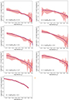 |
Fig. 1. X-ray surface brightness profile as estimated in Popesso et al. (2025a). The solid red line represents the stacked profile, while the pink shaded region indicates the uncertainty derived from bootstrapping. The panel in the last row displays the average X-ray surface brightness profile (solid red line) of the eFEDS detections with optical counterparts in the GAMA galaxy sample, corresponding to the specific halo mass bin, while the pink shaded region indicates the dispersion. The solid purple line in all panels shows the best-fit projected X-ray emissivity profile, represented by ne(r)2Λ(kT, Z). |
To complement our measure at higher halo masses, we use the average fgas profile of the CHEX-MATE cluster subsample used for the stack of eROSITA data by Lyskova et al. (2023). The CHEX-MATE cluster sample (CHEX-MATE Collaboration 2021) is an unbiased, signal-to-noise limited sample of 118 galaxy clusters detected by Planck via the Sunyaev-Zel’dovich effect. It is composed of clusters at z < 0.2 with masses 2 × 10¹⁴ < M500/M⊙ < 9 × 10¹⁴ from the PSZ2 catalog (Planck Collaboration XIII 2016). The CHEX-MATE subsample used for the stacking comprises 38 systems in regions with minimal background variations due to proximity to the Galactic plane and the Cygnus-X star formation region, and relatively far from the North Polar Spur. We derive the mean M200 and R200 from the average M500 and R500 estimates listed in Lyskova et al. (2023), by assuming a NFW profile with concentration of six (see also Dutton & Macciò 2014).
3. The gas mass
3.1. The gas mass estimate
We estimated the gas mass profile as described in Liu et al. (2022a). Specifically, we used a Vikhlinin et al. (2006) electron number density model:
 (1)
(1)
where n0 is the normalization factor, rc and rs are the core and scale radii, β controls the overall slope of the density profile, α controls the slope in the core and at intermediate radii, and ϵ controls the change of slope at large radii. This is used to estimate and integrate along the line of sight the X-ray emissivity, ne(r)2Λ(kT, Z) profile, where Λ(kT, Z) is the cooling function depending on the gas temperature and metallicity. The cooling function is derived by assuming a gas temperature from the M − TX relation of Lovisari et al. (2015) at the mean M500 of the halo mass bin. As in Liu et al. (2022a), we assumed a metallicity of the ICM of 0.3 Z⊙, adopting the solar abundance table of Asplund et al. (2009), that includes the He abundance. This assumption is consistent with the average metallicity estimated in poor cluster cores by Lovisari & Reiprich (2019) and with Magneticum predictions, although the observed scatter is large. The error due to these assumptions is estimated in Popesso et al. (2025b, see also next session) based on the Magneticum mock observations. The effect on X-ray emissivity depends mainly on the systematics of the halo mass proxy. For the GAMA group sample, the use of the total luminosity proxy results in a scatter of 40% in the emissivity estimate at fixed metallicity. The assumption of a fixed metallicity of 0.3 Z⊙ leads to a variation in emissivity of 37%. Since these effects cannot be corrected, they are included in the error budget and summed in quadrature with the statistical errors.
The projected number density model is convolved with the eROSITA PSF and fit to the data. Differently from Liu et al. (2022a) we leave all parameters free in the fit, but ϵ, which rules the change of slope at large radii. This is poorly constrained due to the relatively low S/N in the outskirts region. Thus, we fixed the value to the cluster value provided by Vikhlinin et al. (2006). Only for the average profile of the detected poor clusters at 14 < log(M200/M⊙) < 14.3, the S/N is high enough to constrain the change of slope at large radii. The best-fit line to the X-ray surface brightness profiles and the best-fit parameters are reported in Fig. 1 and Table 1, respectively. The electron density profiles obtained in this way are shown in Fig. 2. We include also the profiles of Lyskova et al. (2023) for the CHEX-MATE clusters.
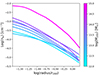 |
Fig. 2. Electron density profiles of groups and clusters in the halo mass bins studied here. The profiles are color coded as a function of M200 as shown in the color bar. The magenta profile is obtained from the stacking in eROSITA of the CHEXMATE clusters, and it was taken from Lyskova et al. (2023). |
Best-fit electron density model parameters of the Vikhlinin et al. (2006).
We computed the ICM mass of a system within a given aperture, by using the best-fit model for the electron density profile,
 (2)
(2)
where the average nuclear charge and mass are A ∼ 1.4 and Z ∼ 1.2, and μe = A/Z ∼ 1.17.
3.2. Validation of the stacking procedure, gas mass estimate, and error budget
The stacking procedure used in this work, validated in detail by Popesso et al. (2025b), is tested on a mock dataset generated from the L30 lightcone of the Magneticum simulation. This dataset includes synthetic eROSITA observations down to the eRASS:4 depth (equivalent to two years of exposure) and a GAMA-like spectroscopic galaxy survey. Optical galaxy groups are identified using a Friends-of-Friends (FoF) algorithm, following the implementation by Robotham et al. (2011), and the performance of this method – particularly in terms of completeness and contamination – is extensively evaluated in Marini et al. (2025).
To replicate the analysis pipeline of Popesso et al. (2025a), the mock data are processed using the same halo mass limits, binning strategy, and halo mass proxies as in the real eROSITA-GAMA dataset. This allows for a direct, end-to-end test of the stacking method and gas mass recovery under observational conditions. The validation study in Popesso et al. (2025b) examines key sources of systematic uncertainty: mis-centering between optical and X-ray centroids, contamination from AGN and X-ray binaries (XRBs), optical selection biases, and scatter in the halo mass proxy. Mis-centering effects are found to be minor, with positional offsets typically small compared to the eROSITA PSF. AGN and XRB contributions, which dominate in low-mass halos (M200 < 1013 M⊙), are modeled and subtracted with negligible residual impact on the recovered surface brightness.
In terms of selection reliability, the Robotham et al. (2011) catalog demonstrates sufficient completeness and low contamination across the mass range. For Milky Way–sized halos (Mhalo ∼ 1012–1012.5 M⊙), the group finder captures approximately 60% of true systems. However, systems with central galaxies hosting satellites below the GAMA magnitude limit are missed and appear as isolated galaxies without an estimate of the halo mass proxy. This selection effect is inherent to the survey depth and might introduce a bias at the low-mass end. An additional critical source of uncertainty, identified as dominant in Popesso et al. (2025b), is the scatter and contamination in the halo mass proxy used to define the stacking bins. Lower- or higher-mass halos may be incorrectly assigned to a bin, leading to contamination from fainter or brighter systems. Popesso et al. (2025b) quantifies this contamination for each bin used in our analysis (see their Table 1).
Despite these challenges, the stacking analysis based on the Robotham et al. (2011) mock catalog successfully recovers the input average X-ray surface brightness profiles and corresponding gas density profiles. As shown in Figs. 12 and 13 of Popesso et al. (2025b), the recovered profiles agree within 1σ with the true input profiles of the simulation based on the complete halo population. Throughout the entire range of halo mass, the stacking method does not introduce significant bias, and the underlying Ygas–Mhalo relation is recovered within the observational uncertainties, as shown in Fig. 17 of Popesso et al. (2025b).
The total error budget in the derived gas mass incorporates three main components:
-
Fitting uncertainty: The gas density profiles were fit using a parametric model, and uncertainties are estimated via bootstrapping. This captures the combined effects of statistical noise, background subtraction, and variation in the halo mass proxy.
-
Correction uncertainty: Additional uncertainty arises from modeling and subtracting AGNs and XRBs contributions. The uncertainty was modelled and included following Popesso et al. (2025b).
-
X-ray emissivity uncertainty: The conversion of X-ray surface brightness to gas density depends on assumptions about the gas temperature and metallicity. In this work, temperature was inferred from the TX–Mhalo relation of Lovisari et al. (2015), and metallicity was assumed to be constant at 0.3 Z⊙. As shown in Popesso et al. (2025b), this introduces a systematic uncertainty of up to 40% for the Robotham et al. (2011) case for halos with a temperature below 1 KeV and 20% above this threshold, while it is negligible in the cluster temperature regime.
Assuming that these components are independent, we combined them in quadrature to estimate the total uncertainty. For groups at halo masses below 1013.5 M⊙, the main source of uncertainty remains the bootstrapping error of the stacking and fitting procedure. This comprehensive treatment ensures that both statistical and systematic errors are accounted for in the final gas mass measurements derived from real data.
4. Results
4.1. The gas concentration
To quantify how the shape of the gas profiles varies with system mass, we estimate the gas concentration (cgas) as the ratio of the gas mass within 0.1 R200 to that within R200. Figure 3 shows the variation of gas concentration with halo mass. A clear trend is observed, with gas concentration increasing with mass; specifically, the CHEX-MATE clusters are approximately 2.5 times as concentrated as Milky Way-sized groups, following a dependence of  . This factor is 3 times larger than errors deriving from observational error of the stacking, including the uncertainty due to the estimate of the gas emissivity by assuming the gas temperature and metallicity, as described in the previous section. Additionally, according to the standard hierarchical formation paradigm, dark matter concentration (c200) decreases monotonically with mass (see also Dutton & Macciò 2014). The opposite trend observed for gas concentration suggests the influence of nongravitational processes, most likely AGN feedback.
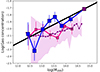 |
Fig. 3. Relation between gas concentration, defined as the ratio of hot gas mass within 0.1 R200 to that within R200, versus halo mass. The blue points represent results derived from the stacked data. The big purple point shows the result based on the electron density profile of the CHEX-MATE clusters stacked in eROSITA (Lyskova et al. 2023). The solid black line represents the best-fit relation based on the combined stacks of eFEDS and CHEX-MATE data. The small purple points indicate the mean relation predicted by the Magneticum simulation, with the shaded region illustrating the dispersion around this relation. The pink squares display the results obtained using the same stacking technique applied in this study to the X-ray surface brightness profiles derived from mock galaxy groups selected using the Robotham et al. (2011) algorithm on the mock eROSITA data from the L30 lightcone of Magneticum. |
We propose that the observed increase in gas concentration from low-mass groups to massive clusters results from AGN feedback evacuating gas more effectively in low-mass halos due to their shallower potential wells compared to clusters. To explore this trend further, we examine the L30 lightcone of the Magneticum simulation, finding a positive correlation with a Spearman coefficient of 0.64 and a probability of no correlation of ∼10−5. However, Magneticum predicts a flatter dependence of  .
.
Figure 3 also presents cgas values obtained by applying the same analysis as in this study to the stacked surface brightness profiles of the mock dataset analogous to the one used here (Marini et al. 2024; Popesso et al. 2025b). Figure 3 shows that our approach, including uncertainties and systematics of the group selection, halo mass proxy choice, and stacking technique, accurately reproduces the cgas − M200 relation predicted by Magneticum within 1σ. This consistency suggests that the results obtained from the observed stacked profiles are robust.
4.2. The observed Ygas − Mhalo relation
We defined the fraction of gas mass within a radius, r, as
 (3)
(3)
where Mgas is estimated from Eq. (2) and Mtot(< r) is the total mass contained within the radius r. In this analysis, we study the gas fraction contained within R500 and R200. We normalize fgas to the universal baryon fraction (Ωb/Ωm = 0.154, Planck Collaboration VI 2020) to obtain Ygas(< r).
Figure 4 shows Ygas estimated within R500 versus M500. The error bars on Ygas are estimated as described in Section 3.2. The median values of M500 and M200, together with their uncertainties for each bin, are taken from Table 1 of Popesso et al. (2025a). This table provides the median and dispersion of the proxy distribution of the halo mass in a mock catalog based on the Robotham et al. (2011) detection algorithm, applied to the input halo populations within the same mass bins used in this analysis. The uncertainties in the median M500 and M200 are calculated by dividing the reported dispersion by the square root of the number of groups included in the stacking. The corresponding error bars are smaller than the symbol size shown in the figure but are included in the fitting procedure. The data points and the corresponding errors are listed in Table 2.
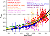 |
Fig. 4. Ygas–M500 relation. The filled circles represent a compilation of literature data, color coded as a function of the sample reference as shown in the picture. The blue squares indicate the Ygas derived from the stacked groups of Popesso et al. (2025a). The purple square indicates the value derived from the CHEXMATE clusters stacked in eROSITA data by Lyskova et al. (2023). The solid black curve represents our best fit to stacked points, including the CHEXMATE clusters. The dashed yellow and green curves represent the best fit of Pratt et al. (2009) and Eckert et al. (2016), respectively. The Ygas = 1 corresponding to the Planck Collaboration VI (2020) value is indicated by the dashed black line. |
Data points of the Ygas − Mhalo relation.
Ygas varies by a factor of ∼10 from M500 ∼ 5 × 10¹² M⊙, Milky Way-sized groups, to M500 ∼ 5 × 10¹⁴ M⊙, the CHEXMATE clusters. The same is observed for Ygas estimated within R200 (see Fig. 5). The best-fit power-law relation to the data, including the CHEXMATE stacked point, is
 (4)
(4)
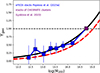 |
Fig. 5. Ygas–M200 relation. The blue squares indicate the Ygas derived from the stacked groups of Popesso et al. (2025a) The purple square indicates the value derived from the CHEXMATE clusters stacked in eROSITA data by Lyskova et al. (2023). The solid black curve represents our best fit to stacked points, including the CHEXMATE clusters. The dashed red line shows the best fit of the Ygas − M500 relation of Fig. 4. |
Our best fit of Eq. (4) is consistent within 1σ with the estimates of Pratt et al. (2009) and Eckert et al. (2016). Nevertheless, it has a similar slope but a lower normalization in comparison to the estimates of Sun et al. (2009), Lovisari et al. (2015), and Eckert et al. (2021). These estimates are based on ROSAT galaxy group samples, that include only the brightest groups of the local Universe due to the high RASS flux limit. The stacked data, instead, are representative of the bulk of the underlying halo mass population as tested in Popesso et al. (2025b) through the analysis of the analog mock dataset generated from Magneticum. Thus, they include also groups and poor clusters whose gas distribution might have been heavily affected by nongravitational processes such as AGN feedback.
In addition to the combination of the eFEDS stacks and the CHEX-MATE stacked point, we also show in Fig. 4 a comprehensive compilation of literature data providing the same estimate for z < 0.2 systems. These are the cluster sample of Mulroy et al. (2019), Mahdavi et al. (2013), Eckert et al. (2019), the REXCESS sample of Pratt et al. (2009), the poor cluster and group sample of Arnaud et al. (2007), Vikhlinin et al. (2006), and Sun et al. (2009) used in Pratt et al. (2009) (APP05 + V09 + S09 in Fig. 4), the XMM-XXL sample of Eckert et al. (2016), the group samples of Gonzalez et al. (2013) and Lovisari et al. (2015), the poor cluster sample of Ragagnin et al. (2022), and the group sample of Rasmussen & Ponman (2009) and Pearson et al. (2017) (RP09 + P17 in Fig. 4). We transformed all the values to our adopted cosmology. We compare the distribution of the literature compilation to our best fit. Given the very different selection functions of the collected data, it is not surprising that they scatter largely around our best fit. Nevertheless, we find consistency in the distribution of the observed systems and the best fit provided here and based on the stacked profiles. In particular, we point out that the XMM-XXL groups of Eckert et al. (2019), which are selected at a flux limit similar to eFEDS, exhibit fgas values consistent with the mean values of the eFEDS detections and stacks at M500 ∼ 1013.5 − 1014 M⊙.
We also present here in Fig. 5, for the very first time, the fgas versus halo mass relation, estimated within R200. Until recently, measuring the fgas beyond R500 was hampered by the lack of sensitivity of previous instruments. The stacking analysis can overcome this problem, as shown by P24 and Lyskova et al. (2023). The combination of eFEDS stacks and the CHEX-MATE stack allows us to determine fgas over the largest halo mass range, and for the largest radius, ever probed so far in groups and clusters. The best-fit relation is
 (5)
(5)
At the Milky Way-sized group scale, fgas is ∼20–40% of the cosmic value. It goes above 50% for massive groups and poor clusters and it reaches the cosmic value at the CHEX-MATE cluster mass scale. The slope of best fit of Eqs. (4) and (5) are consistent within 2σ, but the fraction of gas nearly doubles from R500 to R200.
4.3. Comparison with simulations
We compare the results of our analysis with the predictions of several hydrodynamical simulations, each implementing a different BH feedback model. We consider, in particular, the predictions of MillenniumTNG (Pakmor et al. 2023), FLAMINGO (Schaye et al. 2023), BAHAMAS (McCarthy et al. 2017), SIMBA (Davé et al. 2019), Illustris (Genel et al. 2014), IllustrisTNG (Pillepich et al. 2019), and Magneticum (Dolag et al. 2016).
For MillenniumTNG, FLAMINGO, BAHAMAS, Illustris, and SIMBA, the fgas–M500 relation is provided in the reference paper. We normalize such a relation to the value of Ωb/Ωm according to the cosmology implemented in each simulation. Only for the IllustrisTNG and Magneticum, we derive the fgas − Mhalo relation ourselves. For IllustrisTNG, we select halos in TNG300, corresponding to the largest cosmological box available, including 2 × 25003 particles in a (302.6 cMpc)3 volume. The dark matter (initial gas) particles have mass 5.9 × 10⁷ M⊙ (1.1107 M⊙) and Plummer equivalent softening 1.48 kpc at z = 0. Details on the simulation and the astrophysical subgrid models implemented can be found in Pillepich et al. (2019). We select halos at redshift z = 0 since we find no evolution of the Ygas − Mhalo relation in the redshift range z = 0–0.2 (i.e., the redshift range of the surveys considered here). As for Magneticum, halos are drawn from Box2b/hr which includes a total of 2 × 28803 particles in a volume of (640 h−1 cMpc)3. The dark matter (initial gas) particles have mass 6.9 × 10⁸ h−1 M⊙ (1.4 × 10⁸ h−1 M⊙) and Plummer equivalent softening 3.75 h−1 kpc (3.75 h−1 kpc). We select halos in the last snapshot available at redshift z = 0.25. To further prove the consistency of our investigation, we repeat the analysis with Box2/hr – 2 × 15843 particles in a (352 h−1 cMpc)3 volume – both at z = 0 and z = 0.3 to rule out possible intrinsic redshift evolution of such relation. More details on the simulations and the astrophysical subgrid models implemented can be found in Dolag et al. (2016). In both simulations, we gather a representative sample of clusters and group-size halos by randomly selecting 104 halos with log M500/M⊙ ≥ 12.2 in each simulation. For each of them, we compute the hot gas mass fraction Ygas within R500 and R200 considering all the hot gas particles. We tested a temperature threshold of 106 K, the value commonly adopted for identifying hot gas particles in clusters and sampled by the eROSITA 0.5–2 keV energy band used in the analysis. Such a temperature should still sample most of the hot gas particles for the groups in the mass regime considered in the analysis. Nevertheless, very low-mass groups, at halo masses below 1012 − 12.2 M⊙, typically have lower temperatures. In these cases, this cut-off excluded a large fraction of gas particles, resulting in a lack of statistically robust outcomes for groups, which are anyhow excluded from the analysis.
The result of the comparison is shown in Fig. 6. Compared to our observational results, Ygas is overpredicted at given Mhalo by MillenniumTNG and IllustrisTNG, which apply the same galaxy physical model (see also Pop et al. 2022, for an alternative estimate in IllustrisTNG300). FLAMINGO, and BAHAMAS, which have similar approaches for the BH feedback implementation, are closer to our observed relation, although they do not follow the observed power law, in particular in the Mhalo range 1013.5 − 14.5 M⊙ (see also Salcido et al. 2023). The Magneticum simulation reproduces the observed relation reasonably well, with a slightly higher normalization that remains consistent within 1σ of the observations (see also Angelinelli et al. 2022). SIMBA also shows agreement within 1σ, albeit with slightly lower concordance. In contrast, Illustris exhibits an overly efficient evacuation of gas from halos across all masses. It is important to note that Genel et al. (2014) provides the gas fraction relation for all phases of gas rather than exclusively the hot phase. Consequently, the relation depicted in the bottom-right panel of Fig. 4.3 represents an upper limit to the hot gas-only relation.
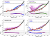 |
Fig. 6. Comparison of the observed Ygas versus mass relations within R500 with different hydrodynamical simulations. The color code for each dataset is indicated in each panel. The light orange squares show the stacked points of Fig. 4, while the black line shows our best-fit relation. The bottom subpanels show the residuals of each dataset to our best fit. These are expressed in dex (log(fgas)−log(fit)). Top-left panel: Comparison of Ygas–M500 relation with the predictions of the BAHAMAS (Salcido et al. 2023) and FLAMINGO (Schaye et al. 2023) simulations. The blue shaded region indicates the 1σ uncertainty of the relation in FLAMINGO as reported in the corresponding paper. These two simulations use similar galaxy evolution models and feedback implementations. Top-right panel: Comparison of Ygas–M500 relation with the predictions of the IllustrisTNG (Pillepich et al. 2019) and of MillenniumTNG (Pakmor et al. 2023) simulations. For IllustrisTNG we show the individual estimates (pink points) and the mean relation (purple squares). For MillenniumTNG we report the mean relation (green squares) retrieved in the corresponding paper. These two simulations use similar galaxy evolution models and feedback implementations. Bottom-left panel: Comparison of Ygas–M500 relation with the predictions of the Magneticum (Dolag et al. 2016). The pink points indicate the individual estimates, while the purple squares indicate the mean relation. Bottom-right panel: Comparison of Ygas–M500 relation with the predictions of the Simba (Davé et al. 2019) and Illustris (Genel et al. 2014). |
The mass range of 1013.5 − 1014 M⊙, where most predictions deviate most significantly from the observed relation, warrants further investigation. To this end, we compare the electron density profiles derived from our stacking analysis to predictions from simulations. For Magneticum, the electron density profile is obtained directly from simulation data, while other profiles are taken from the review by Oppenheimer et al. (2021). As shown in Fig. 7, the profiles from Magneticum and SIMBA align most closely with the observations. In contrast, the normalizations of the EAGLE (Schaye et al. 2015) and IllustrisTNG simulations exceed observational results by a factor of approximately three. These results are more consistent with those from studies of bright X-ray groups, which naturally contain a higher gas fraction (e.g., Lovisari et al. 2015; Sun et al. 2009).
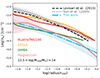 |
Fig. 7. Electron density profile for groups at 1013 M⊙ < M200 < 1014 M⊙ from this work (blue dashed-dotted curve), Lovisari et al. (2015) (black dashed curve) and Sun et al. (2009) (gray dotted curve), compared with the predictions of the hydrodynamical simulations in the same M200 mass bin: Magneticum (pink curve), IllustrisTNG100 (red curve), EAGLE (orange curve), and Simba (green curve). With the exclusion of the Magneticum data provided by Popesso et al. (2025b), the profiles of the simulations are taken from the review of Oppenheimer et al. (2021). |
The discrepancies among simulations are largely attributable to differences in the treatment of galaxy formation physics and the associated timing and effects of black hole feedback on the intracluster medium (ICM). These variations make it challenging to isolate specific drivers of the observed differences, as they likely arise from a combination of factors. For example, Kauffmann et al. (2019) provide a compelling illustration of this complexity through a trace particle analysis comparing Illustris (Nelson et al. 2015) and IllustrisTNG. Their study demonstrates that Illustris evacuates hot gas from galaxy groups more effectively than IllustrisTNG (see also Hadzhiyska et al. 2025). The findings by Kauffmann et al. (2019) attribute these differences to the subgrid models of feedback, which affect the timing of gas displacement, cooling, and collapse during galaxy evolution, in addition to switching from a thermal to a kinetic AGN feedback at low accretion rates (in the radio mode). However, the observed differences in the dependence on group or cluster mass suggest that an important factor may be the inclusion (or lack thereof) of halo mass-dependent feedback parameters. For instance, kinetic feedback models vary across simulations and are absent in Magneticum, which could play a critical role in shaping the observed trends.
4.4. Comparison with eRASS:1 data
To further validate our findings, we compare them with a subsample of groups and clusters selected from eRASS:1 observations as presented by Bulbul et al. (2024). This subsample, illustrated in Fig. 8, comprises all clusters and groups at z < 0.05 with a well-defined optical counterpart in the matched catalog provided in the eRASS:1 data release, as described by Bulbul et al. (2024). These systems include only those with more than five spectroscopic members. A flux cut of 10−13.5 erg s−1 cm−2 was applied to ensure a 50% complete sample for systems with M500 > 6 × 10¹³ M⊙, following the completeness criteria outlined by Bulbul et al. (2024). Additionally, Fig. 8 includes systems with masses below this completeness limit.
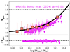 |
Fig. 8. Upper panel: Comparison of the observed Ygas versus mass relations within R500 with the fgas values within the same radius as given by Bulbul et al. (2024) for the eRASS:1 extended objects at z < 0.05 and with an optical counterpart. Lower panel: Residuals of the eRASS:1 data from the best fit of Fig. 4 expressed in dex (log(fgas)−log(fit)). |
The gas masses reported by Bulbul et al. (2024) were estimated using the methodology described in Liu et al. (2022a), which was previously applied to eFEDS-detected systems. Total masses were derived using scaling relations calibrated with weak lensing mass estimates (see Bulbul et al. 2024, for further details). In these analyses, eROSITA data were simultaneously fit to extract M500 and temperature, iteratively refining the aperture size to define R500 such that the data aligned with the observed LX − M500 scaling relation. As a result, all derived measurements are inherently correlated.
Despite these correlations, we find excellent agreement between our best-fit fgas − Mhalo relation and the independent estimates from Bulbul et al. (2024). This consistency further underscores the robustness of our results and strengthens confidence in the methodologies employed.
5. Discussion and conclusion
Using the stacking results from optically selected groups in eFEDS and the eROSITA stacked surface brightness profile of the CHEX-MATE clusters, we provide a comprehensive measurement of the fgas − Mhalo relation over the largest halo mass range and to the largest radii ever probed for galaxy systems at z < 0.2. Extensive tests conducted on an analogous mock dataset ensure that our results are robust against selection biases. We find that the fgas − Mhalo relation is well-described by a power law with a consistent shape (within 1 − 2σ) when estimated within both R500 and R200 radii. This relation is in agreement with other studies that utilize X-ray survey data of similar depth, such as eFEDS and XXM-XXL (see, e.g., Eckert et al. 2016). However, our results indicate a lower fgas in the group regime compared to studies based on X-ray bright groups (e.g., Sun et al. 2009; Lovisari et al. 2015; Eckert et al. 2021). We interpret this discrepancy as a selection effect, with X-ray brightest nearby groups occupying the upper envelope of the fgas − Mhalo relation at fixed halo mass.
Comparing our observed fgas − Mhalo relation with predictions from various hydrodynamical simulations reveals that most current state-of-the-art models tend to overpredict the gas fraction across different halo mass ranges. Only Magneticum and, to a lesser extent, SIMBA align with the observed relation. Interestingly, the most significant discrepancies are not evident at the Milky Way group mass scale, where simulations generally perform well, but rather at the scale of massive groups and poor clusters (13.5 < log(M500/M⊙) < 14.3). These discrepancies are unlikely to arise from systematic biases in our fgas measurements, as our best-fit relation aligns well with literature data compilations (Fig. 4). Instead, while Magneticum and SIMBA accurately reproduce the electron density profiles derived from the data, EAGLE and IllustrisTNG overestimate the normalization of these profiles, leading to an overprediction of gas mass fractions.
The low fgas values observed at the group mass scale, approximately 0–40% of the cosmic baryon fraction, suggest that a significant portion of the hot gas may reside beyond the virial region or exist in non-X-ray-emitting phases. Simulations predominantly support the first scenario, where feedback mechanisms expel gas to regions far beyond the virial radius, particularly in lower-mass halos. Studies such as Angelinelli et al. (2022) and Ayromlou et al. (2023) demonstrate that in both Magneticum and IllustrisTNG, most baryons in the form of hot gas are displaced well beyond the virial radius in Milky Way-sized halos and massive groups. This displacement implies that the halo closure radius – where baryon content aligns with the cosmic value – extends significantly beyond R200 for most group-sized systems. However, in IllustrisTNG, this gas expulsion is insufficient at the massive group and poor cluster scales, where our observations reveal discrepancies in fgas of up to a factor of three. This may indicate that the moderated or halo-mass-dependent feedback in IllustrisTNG, introduced to better match galaxy properties (Pillepich et al. 2019), does not expel gas as efficiently as the original Illustris model (Nelson et al. 2015).
This discrepancy is further highlighted in Hadzhiyska et al. (2025), which reports kinematic Sunyaev-Zeldovich (kSZ) effect measurements from the Atacama Cosmology Telescope (ACT), stacked on the luminous red galaxy (LRG) sample of the Dark Energy Spectroscopic Instrument (DESI). These observations detect gas extending well beyond the virial radius at high significance (> 40σ), showing better agreement with Illustris predictions than with IllustrisTNG (see also Amodeo et al. 2021). It is worth noting that the feedback adjustments in IllustrisTNG improve predicted galaxy properties, such as color and star formation rates, compared to Illustris (Sparre et al. 2015; Donnari et al. 2021). However, these adjustments appear to compromise the accuracy of gas distribution predictions within halos. Similarly, while Magneticum performs well in reproducing halo gas properties (see also Popesso et al. 2025b,a), it overquenches local galaxy populations (Mazengo et al., in prep.), as does SIMBA (Davé et al. 2019).
Other simulations, such as BAHAMAS and FLAMINGO, exhibit less extreme behavior compared to IllustrisTNG. While they do not perfectly reproduce the fgas − Mhalo relation, the maximum disagreement is limited to a factor of two at M500 ∼ 1014 M⊙. Additionally, their galaxy populations do not suffer from the strong overquenching of star formation observed in Magneticum, or SIMBA, although their lower resolution poses limitations compared to these simulations (Schaye et al. 2023; McCarthy et al. 2017).
We conclude that current hydrodynamical simulations face a critical challenge in balancing subgrid physics. While strong feedback mechanisms effectively expel gas from halos, they often suppress star formation too aggressively, leading to inconsistencies in modeling galaxy populations. The critical challenge lies not only in determining the magnitude of energy feedback required to deplete or prevent gas cooling and inflow but also in understanding when and where these processes occur. Addressing this requires robust observational constraints on halo gas and galaxy properties across cosmic time and varying environments, which remain largely lacking.
In conclusion, our estimates of fgas over a wide range of halo masses, from Milky Way-sized groups to clusters, and out to R200 distances, set severe constraints to theoretical models that investigate the co-evolution of the hot intra-group medium in the presence of the central galaxy BH feedback, and highlights the importance of avoiding selection biases when deriving halo properties that can depend on the halo selection process itself.
Acknowledgments
PP acknowledges financial support from the European Research Council (ERC) under the European Union’s Horizon Europe research and innovation programme ERC CoG CLEVeR (Grant agreement No. 101045437). AB acknowledges the financial contribution from the INAF mini-grant 1.05.12.04.01 “The dynamics of clusters of galaxies from the projected phase-space distribution of cluster galaxies”. KD acknowledges support by the COMPLEX project from the European Research Council (ERC) under the European Union’s Horizon 2020 research and innovation program grant agreement ERC-2019-AdG 882679. The calculations for the Magneticum simulations were carried out at the Leibniz Supercomputer Center (LRZ) under the project pr83li. GP acknowledges financial support from the European Research Council (ERC) under the European Union’s Horizon 2020 research and innovation program Hot- Milk (grant agreement No 865637), support from Bando per il Finanziamento della Ricerca Fondamentale 2022 dell’Istituto Nazionale di Astrofisica (INAF): GO Large program and from the Framework per l’Attrazione e il Rafforzamento delle Eccellenze (FARE) per la ricerca in Italia (R20L5S39T9). SVZ and VB acknowledge support by the Deutsche Forschungsgemeinschaft, DFG project nr. 415510302 This work is based on data from eROSITA, the soft X-ray instrument aboard SRG, a joint Russian-German science mission supported by the Russian Space Agency (Roskosmos), in the interests of the Russian Academy of Sciences represented by its Space Research Institute (IKI), and the Deutsches Zentrum für Luft- und Raumfahrt (DLR). The SRG spacecraft was built by Lavochkin Association (NPOL) and its subcontractors and is operated by NPOL with support from the Max Planck Institute for Extraterrestrial Physics (MPE). The development and construction of the eROSITA X-ray instrument was led by MPE, with contributions from the Dr. Karl Remeis Observatory Bamberg & ECAP (FAU Erlangen-Nuernberg), the University of Hamburg Observatory, the Leibniz Institute for Astrophysics Potsdam (AIP), and the Institute for Astronomy and Astrophysics of the University of Tübingen, with the support of DLR and the Max Planck Society. The Argelander Institute for Astronomy of the University of Bonn and the Ludwig Maximilians Universität Munich also participated in the science preparation for eROSITA. The eROSITA data shown here were processed using the eSASS software system developed by the German eROSITA consortium. GAMA is a joint European-Australasian project based around a spectroscopic campaign using the Anglo-Australian Telescope. The GAMA input catalog is based on data taken from the Sloan Digital Sky Survey and the UKIRT Infrared Deep Sky Survey. Complementary imaging of the GAMA regions is being obtained by a number of independent survey programmes including GALEX MIS, VST KiDS, VISTA VIKING, WISE, Herschel-ATLAS, GMRT and ASKAP providing UV to radio coverage. GAMA is funded by the STFC (UK), the ARC (Australia), the AAO, and the participating institutions. The GAMA website is https://www.gama-survey.org.
References
- Amodeo, S., Battaglia, N., Schaan, E., et al. 2021, Phys. Rev. D, 103, 063514 [NASA ADS] [CrossRef] [Google Scholar]
- Anderson, M. E., Gaspari, M., White, S. D. M., Wang, W., & Dai, X. 2015, MNRAS, 449, 3806 [NASA ADS] [CrossRef] [Google Scholar]
- Angelinelli, M., Ettori, S., Dolag, K., Vazza, F., & Ragagnin, A. 2022, A&A, 663, L6 [NASA ADS] [CrossRef] [EDP Sciences] [Google Scholar]
- Arnaud, M., Pointecouteau, E., & Pratt, G. W. 2007, A&A, 474, L37 [CrossRef] [EDP Sciences] [Google Scholar]
- Asplund, M., Grevesse, N., Sauval, A. J., & Scott, P. 2009, ARA&A, 47, 481 [NASA ADS] [CrossRef] [Google Scholar]
- Ayromlou, M., Nelson, D., & Pillepich, A. 2023, MNRAS, 524, 5391 [CrossRef] [Google Scholar]
- Bahar, Y. E., Bulbul, E., Clerc, N., et al. 2022, A&A, 661, A7 [NASA ADS] [CrossRef] [EDP Sciences] [Google Scholar]
- Biffi, V., Dolag, K., & Merloni, A. 2018, MNRAS, 481, 2213 [Google Scholar]
- Blanton, M. R., Bershady, M. A., Abolfathi, B., et al. 2017, AJ, 154, 28 [Google Scholar]
- Brunner, H., Liu, T., Lamer, G., et al. 2022, A&A, 661, A1 [NASA ADS] [CrossRef] [EDP Sciences] [Google Scholar]
- Bulbul, E., Chiu, I. N., Mohr, J. J., et al. 2019, ApJ, 871, 50 [Google Scholar]
- Bulbul, E., Liu, A., Pasini, T., et al. 2022, A&A, 661, A10 [NASA ADS] [CrossRef] [EDP Sciences] [Google Scholar]
- Bulbul, E., Liu, A., Kluge, M., et al. 2024, A&A, 685, A106 [NASA ADS] [CrossRef] [EDP Sciences] [Google Scholar]
- CHEX-MATE Collaboration (Arnaud, M., et al.) 2021, A&A, 650, A104 [NASA ADS] [CrossRef] [EDP Sciences] [Google Scholar]
- Crossett, J. P., McGee, S. L., Ponman, T. J., et al. 2022, A&A, 663, A2 [Google Scholar]
- Davé, R., Anglés-Alcázar, D., Narayanan, D., et al. 2019, MNRAS, 486, 2827 [Google Scholar]
- Dolag, K., Komatsu, E., & Sunyaev, R. 2016, MNRAS, 463, 1797 [Google Scholar]
- Donnari, M., Pillepich, A., Nelson, D., et al. 2021, MNRAS, 506, 4760 [NASA ADS] [CrossRef] [Google Scholar]
- Driver, S. P., Bellstedt, S., Robotham, A. S. G., et al. 2022, MNRAS, 513, 439 [NASA ADS] [CrossRef] [Google Scholar]
- Dutton, A. A., & Macciò, A. V. 2014, MNRAS, 441, 3359 [Google Scholar]
- Eckert, D., Ettori, S., Coupon, J., et al. 2016, A&A, 592, A12 [NASA ADS] [CrossRef] [EDP Sciences] [Google Scholar]
- Eckert, D., Ghirardini, V., Ettori, S., et al. 2019, A&A, 621, A40 [NASA ADS] [CrossRef] [EDP Sciences] [Google Scholar]
- Eckert, D., Gaspari, M., Gastaldello, F., Le Brun, A. M. C., & O’Sullivan, E. 2021, Universe, 7, 142 [NASA ADS] [CrossRef] [Google Scholar]
- Ettori, S. 2015, MNRAS, 446, 2629 [NASA ADS] [CrossRef] [Google Scholar]
- Fabjan, D., Borgani, S., Tornatore, L., et al. 2010, MNRAS, 401, 1670 [Google Scholar]
- Galárraga-Espinosa, D., Langer, M., & Aghanim, N. 2022, A&A, 661, A115 [NASA ADS] [CrossRef] [EDP Sciences] [Google Scholar]
- Genel, S., Vogelsberger, M., Springel, V., et al. 2014, MNRAS, 445, 175 [Google Scholar]
- Giles, P. A., Robotham, A., Ramos-Ceja, M. E., et al. 2022, MNRAS, 511, 1227 [Google Scholar]
- Gonzalez, A. H., Sivanandam, S., Zabludoff, A. I., & Zaritsky, D. 2013, ApJ, 778, 14 [Google Scholar]
- Hadzhiyska, B., Ferraro, S., Ried Guachalla, B., et al. 2025, Phys. Rev. D, 112, 083509 [Google Scholar]
- Kauffmann, G., Nelson, D., Borthakur, S., et al. 2019, MNRAS, 486, 4686 [NASA ADS] [CrossRef] [Google Scholar]
- Klein, M., Oguri, M., Mohr, J. J., et al. 2022, A&A, 661, A4 [NASA ADS] [CrossRef] [EDP Sciences] [Google Scholar]
- Le Brun, A. M. C., McCarthy, I. G., Schaye, J., & Ponman, T. J. 2014, MNRAS, 441, 1270 [NASA ADS] [CrossRef] [Google Scholar]
- Liu, A., Bulbul, E., Ghirardini, V., et al. 2022a, A&A, 661, A2 [NASA ADS] [CrossRef] [EDP Sciences] [Google Scholar]
- Liu, T., Buchner, J., Nandra, K., et al. 2022b, A&A, 661, A5 [NASA ADS] [CrossRef] [EDP Sciences] [Google Scholar]
- Lovisari, L., & Ettori, S. 2021, Universe, 7, 254 [NASA ADS] [CrossRef] [Google Scholar]
- Lovisari, L., & Reiprich, T. H. 2019, MNRAS, 483, 540 [Google Scholar]
- Lovisari, L., Reiprich, T. H., & Schellenberger, G. 2015, A&A, 573, A118 [NASA ADS] [CrossRef] [EDP Sciences] [Google Scholar]
- Lyskova, N., Churazov, E., Khabibullin, I. I., et al. 2023, MNRAS, 525, 898 [NASA ADS] [CrossRef] [Google Scholar]
- Mahdavi, A., Hoekstra, H., Babul, A., et al. 2013, ApJ, 767, 116 [NASA ADS] [CrossRef] [Google Scholar]
- Mantz, A. B., von der Linden, A., Allen, S. W., et al. 2015, MNRAS, 446, 2205 [Google Scholar]
- Marini, I., Popesso, P., Lamer, G., et al. 2024, A&A, 689, A7 [NASA ADS] [CrossRef] [EDP Sciences] [Google Scholar]
- Marini, I., Popesso, P., Dolag, K., et al. 2025, A&A, 694, A207 [NASA ADS] [CrossRef] [EDP Sciences] [Google Scholar]
- McCarthy, I. G., Schaye, J., Ponman, T. J., et al. 2010, MNRAS, 406, 822 [NASA ADS] [Google Scholar]
- McCarthy, I. G., Schaye, J., Bird, S., & Le Brun, A. M. C. 2017, MNRAS, 465, 2936 [Google Scholar]
- Mulchaey, J. S. 2000, ARA&A, 38, 289 [NASA ADS] [CrossRef] [Google Scholar]
- Mulroy, S. L., Farahi, A., Evrard, A. E., et al. 2019, MNRAS, 484, 60 [NASA ADS] [CrossRef] [Google Scholar]
- Navarro, J. F., Frenk, C. S., & White, S. D. M. 1997, ApJ, 490, 493 [Google Scholar]
- Nelson, D., Pillepich, A., Genel, S., et al. 2015, Astron. Comput., 13, 12 [Google Scholar]
- Nugent, J. M., Dai, X., & Sun, M. 2020, ApJ, 899, 160 [NASA ADS] [CrossRef] [Google Scholar]
- Oppenheimer, B. D., Babul, A., Bahé, Y., Butsky, I. S., & McCarthy, I. G. 2021, Universe, 7, 209 [NASA ADS] [CrossRef] [Google Scholar]
- Osmond, J. P. F., & Ponman, T. J. 2004, MNRAS, 350, 1511 [NASA ADS] [CrossRef] [Google Scholar]
- Pakmor, R., Springel, V., Coles, J. P., et al. 2023, MNRAS, 524, 2539 [NASA ADS] [CrossRef] [Google Scholar]
- Pearson, R. J., Ponman, T. J., Norberg, P., et al. 2017, MNRAS, 469, 3489 [CrossRef] [Google Scholar]
- Peebles, P. J. E. 1980, The Large-Scale Structure of the Universe (Princeton University Press) [Google Scholar]
- Pillepich, A., Nelson, D., Springel, V., et al. 2019, MNRAS, 490, 3196 [Google Scholar]
- Planck Collaboration VI. 2020, A&A, 641, A6 [NASA ADS] [CrossRef] [EDP Sciences] [Google Scholar]
- Planck Collaboration XIII. 2016, A&A, 594, A13 [NASA ADS] [CrossRef] [EDP Sciences] [Google Scholar]
- Ponman, T. J., Bourner, P. D. J., & Ebeling, H. 1996, in Roentgenstrahlung from the Universe, eds. H. U. Zimmermann, J. Trümper, & H. Yorke, 357 [Google Scholar]
- Pop, A. R., Hernquist, L., Nagai, D., et al. 2022, arXiv e-prints [arXiv:2205.11528] [Google Scholar]
- Popesso, P., Biviano, A., Böhringer, H., Romaniello, M., & Voges, W. 2005, A&A, 433, 431 [NASA ADS] [CrossRef] [EDP Sciences] [Google Scholar]
- Popesso, P., Biviano, A., Bulbul, E., et al. 2024, MNRAS, 527, 895 [Google Scholar]
- Popesso, P., Marini, I., Dolag, K., et al. 2025a, A&A, 704, A278 [NASA ADS] [CrossRef] [EDP Sciences] [Google Scholar]
- Popesso, P., Marini, I., Dolag, K., et al. 2025b, A&A, 704, A277 [NASA ADS] [CrossRef] [EDP Sciences] [Google Scholar]
- Pratt, G. W., Croston, J. H., Arnaud, M., & Böhringer, H. 2009, A&A, 498, 361 [NASA ADS] [CrossRef] [EDP Sciences] [Google Scholar]
- Puchwein, E., Sijacki, D., & Springel, V. 2008, ApJ, 687, L53 [NASA ADS] [CrossRef] [Google Scholar]
- Ragagnin, A., Andreon, S., & Puddu, E. 2022, A&A, 666, A22 [NASA ADS] [CrossRef] [EDP Sciences] [Google Scholar]
- Rasmussen, J., & Ponman, T. J. 2009, MNRAS, 399, 239 [Google Scholar]
- Robotham, A. S. G., Norberg, P., Driver, S. P., et al. 2011, MNRAS, 416, 2640 [NASA ADS] [CrossRef] [Google Scholar]
- Rozo, E., Rykoff, E. S., Evrard, A., et al. 2009, ApJ, 699, 768 [CrossRef] [Google Scholar]
- Rykoff, E. S., McKay, T. A., Becker, M. R., et al. 2008, ApJ, 675, 1106 [NASA ADS] [CrossRef] [Google Scholar]
- Salcido, J., McCarthy, I. G., Kwan, J., Upadhye, A., & Font, A. S. 2023, MNRAS, 523, 2247 [NASA ADS] [CrossRef] [Google Scholar]
- Salvato, M., Wolf, J., Dwelly, T., et al. 2022, A&A, 661, A3 [NASA ADS] [CrossRef] [EDP Sciences] [Google Scholar]
- Schaye, J., Crain, R. A., Bower, R. G., et al. 2015, MNRAS, 446, 521 [Google Scholar]
- Schaye, J., Kugel, R., Schaller, M., et al. 2023, MNRAS, 526, 4978 [NASA ADS] [CrossRef] [Google Scholar]
- Sijacki, D., Springel, V., Di Matteo, T., & Hernquist, L. 2007, MNRAS, 380, 877 [NASA ADS] [CrossRef] [Google Scholar]
- Sparre, M., Hayward, C. C., Springel, V., et al. 2015, MNRAS, 447, 3548 [Google Scholar]
- Sun, M., Voit, G. M., Donahue, M., et al. 2009, ApJ, 693, 1142 [NASA ADS] [CrossRef] [Google Scholar]
- Tempel, E., Tuvikene, T., Kipper, R., & Libeskind, N. I. 2017, A&A, 602, A100 [NASA ADS] [CrossRef] [EDP Sciences] [Google Scholar]
- Vallés-Pérez, D., Planelles, S., & Quilis, V. 2020, MNRAS, 499, 2303 [CrossRef] [Google Scholar]
- Vikhlinin, A., Kravtsov, A., Forman, W., et al. 2006, ApJ, 640, 691 [Google Scholar]
- Vikhlinin, A., Kravtsov, A. V., Burenin, R. A., et al. 2009, ApJ, 692, 1060 [Google Scholar]
- Vulic, N., Hornschemeier, A. E., Haberl, F., et al. 2022, A&A, 661, A16 [NASA ADS] [CrossRef] [EDP Sciences] [Google Scholar]
- Yang, X., Mo, H. J., van den Bosch, F. C., et al. 2007, ApJ, 671, 153 [Google Scholar]
- Zhang, Y., Comparat, J., Ponti, G., et al. 2024, A&A, 690, A268 [NASA ADS] [CrossRef] [EDP Sciences] [Google Scholar]
RΔ represents the radius of a sphere centered on the group, with a mean density equal to Δ times the critical density of the Universe at the group’s redshift.
All Tables
All Figures
|
Fig. 1. X-ray surface brightness profile as estimated in Popesso et al. (2025a). The solid red line represents the stacked profile, while the pink shaded region indicates the uncertainty derived from bootstrapping. The panel in the last row displays the average X-ray surface brightness profile (solid red line) of the eFEDS detections with optical counterparts in the GAMA galaxy sample, corresponding to the specific halo mass bin, while the pink shaded region indicates the dispersion. The solid purple line in all panels shows the best-fit projected X-ray emissivity profile, represented by ne(r)2Λ(kT, Z). |
| In the text | |
|
Fig. 2. Electron density profiles of groups and clusters in the halo mass bins studied here. The profiles are color coded as a function of M200 as shown in the color bar. The magenta profile is obtained from the stacking in eROSITA of the CHEXMATE clusters, and it was taken from Lyskova et al. (2023). |
| In the text | |
|
Fig. 3. Relation between gas concentration, defined as the ratio of hot gas mass within 0.1 R200 to that within R200, versus halo mass. The blue points represent results derived from the stacked data. The big purple point shows the result based on the electron density profile of the CHEX-MATE clusters stacked in eROSITA (Lyskova et al. 2023). The solid black line represents the best-fit relation based on the combined stacks of eFEDS and CHEX-MATE data. The small purple points indicate the mean relation predicted by the Magneticum simulation, with the shaded region illustrating the dispersion around this relation. The pink squares display the results obtained using the same stacking technique applied in this study to the X-ray surface brightness profiles derived from mock galaxy groups selected using the Robotham et al. (2011) algorithm on the mock eROSITA data from the L30 lightcone of Magneticum. |
| In the text | |
|
Fig. 4. Ygas–M500 relation. The filled circles represent a compilation of literature data, color coded as a function of the sample reference as shown in the picture. The blue squares indicate the Ygas derived from the stacked groups of Popesso et al. (2025a). The purple square indicates the value derived from the CHEXMATE clusters stacked in eROSITA data by Lyskova et al. (2023). The solid black curve represents our best fit to stacked points, including the CHEXMATE clusters. The dashed yellow and green curves represent the best fit of Pratt et al. (2009) and Eckert et al. (2016), respectively. The Ygas = 1 corresponding to the Planck Collaboration VI (2020) value is indicated by the dashed black line. |
| In the text | |
|
Fig. 5. Ygas–M200 relation. The blue squares indicate the Ygas derived from the stacked groups of Popesso et al. (2025a) The purple square indicates the value derived from the CHEXMATE clusters stacked in eROSITA data by Lyskova et al. (2023). The solid black curve represents our best fit to stacked points, including the CHEXMATE clusters. The dashed red line shows the best fit of the Ygas − M500 relation of Fig. 4. |
| In the text | |
|
Fig. 6. Comparison of the observed Ygas versus mass relations within R500 with different hydrodynamical simulations. The color code for each dataset is indicated in each panel. The light orange squares show the stacked points of Fig. 4, while the black line shows our best-fit relation. The bottom subpanels show the residuals of each dataset to our best fit. These are expressed in dex (log(fgas)−log(fit)). Top-left panel: Comparison of Ygas–M500 relation with the predictions of the BAHAMAS (Salcido et al. 2023) and FLAMINGO (Schaye et al. 2023) simulations. The blue shaded region indicates the 1σ uncertainty of the relation in FLAMINGO as reported in the corresponding paper. These two simulations use similar galaxy evolution models and feedback implementations. Top-right panel: Comparison of Ygas–M500 relation with the predictions of the IllustrisTNG (Pillepich et al. 2019) and of MillenniumTNG (Pakmor et al. 2023) simulations. For IllustrisTNG we show the individual estimates (pink points) and the mean relation (purple squares). For MillenniumTNG we report the mean relation (green squares) retrieved in the corresponding paper. These two simulations use similar galaxy evolution models and feedback implementations. Bottom-left panel: Comparison of Ygas–M500 relation with the predictions of the Magneticum (Dolag et al. 2016). The pink points indicate the individual estimates, while the purple squares indicate the mean relation. Bottom-right panel: Comparison of Ygas–M500 relation with the predictions of the Simba (Davé et al. 2019) and Illustris (Genel et al. 2014). |
| In the text | |
|
Fig. 7. Electron density profile for groups at 1013 M⊙ < M200 < 1014 M⊙ from this work (blue dashed-dotted curve), Lovisari et al. (2015) (black dashed curve) and Sun et al. (2009) (gray dotted curve), compared with the predictions of the hydrodynamical simulations in the same M200 mass bin: Magneticum (pink curve), IllustrisTNG100 (red curve), EAGLE (orange curve), and Simba (green curve). With the exclusion of the Magneticum data provided by Popesso et al. (2025b), the profiles of the simulations are taken from the review of Oppenheimer et al. (2021). |
| In the text | |
|
Fig. 8. Upper panel: Comparison of the observed Ygas versus mass relations within R500 with the fgas values within the same radius as given by Bulbul et al. (2024) for the eRASS:1 extended objects at z < 0.05 and with an optical counterpart. Lower panel: Residuals of the eRASS:1 data from the best fit of Fig. 4 expressed in dex (log(fgas)−log(fit)). |
| In the text | |
Current usage metrics show cumulative count of Article Views (full-text article views including HTML views, PDF and ePub downloads, according to the available data) and Abstracts Views on Vision4Press platform.
Data correspond to usage on the plateform after 2015. The current usage metrics is available 48-96 hours after online publication and is updated daily on week days.
Initial download of the metrics may take a while.