| Issue |
A&A
Volume 707, March 2026
|
|
|---|---|---|
| Article Number | A170 | |
| Number of page(s) | 12 | |
| Section | Numerical methods and codes | |
| DOI | https://doi.org/10.1051/0004-6361/202554026 | |
| Published online | 11 March 2026 | |
Generalizing across astronomical surveys: Few-shot light curve classification with Astromer 2
1
Department of Computer Science, Universidad de Concepción,
Edmundo Larenas 219,
Concepción,
Chile
2
John A. Paulson School of Engineering and Applied Science, Harvard University,
Cambridge,
MA
02138,
USA
3
Center for Data and Artificial Intelligence, Universidad de Concepción,
Edmundo Larenas 310,
Concepción,
Chile
4
Millennium Institute of Astrophysics (MAS),
Nuncio Monseñor Sotero Sanz 100, Of. 104, Providencia,
Santiago,
Chile
5
Millennium Nucleus on Young Exoplanets and their Moons (YEMS),
Chile
6
Heidelberg Institute for Theoretical Studies, Heidelberg,
Baden-Württemberg,
Germany
★ Corresponding author: This email address is being protected from spambots. You need JavaScript enabled to view it.
Received:
4
February
2025
Accepted:
5
January
2026
Abstract
Context. Foundational models have emerged as a powerful paradigm within the deep learning field. Their capacity relies on the ability to learn robust representations from large-scale datasets and generalize to diverse downstream applications, such as classification. In this paper, we present Astromer 2, a foundational model designed for extracting light curve embeddings.
Aims. We introduce Astromer 2, an enhanced iteration of our self-supervised model for light curve analysis. This paper highlights the advantages of its pretrained embeddings, compares its performance with that of its predecessor, Astromer 1, and provides a detailed empirical analysis of its capabilities, offering deeper insights into the model’s representations.
Methods. Astromer 2 is pretrained on 1.5 million single-band light curves from the MACHO survey using a self-supervised learning task that predicts randomly masked observations within sequences. Finetuning on a smaller labeled dataset allows us to assess its performance in classification tasks. The quality of the embeddings is measured by the F1 score of an multilayer perceptron (MLP) classifier trained on Astromer-generated embeddings.
Results. Our results demonstrate that Astromer 2 significantly outperforms Astromer 1 across all evaluated scenarios, including limited datasets of 20,100, and 500 samples per class. The use of weighted per-sample embeddings, which integrate intermediate representations from Astromer’s attention blocks, is particularly impactful. Notably, Astromer 2 achieves a 15% improvement in F1 score on the ATLAS dataset compared to prior models, showcasing robust generalization to new datasets. This enhanced performance, especially with minimal labeled data, underscores the potential of Astromer 2 for more efficient and scalable light curve analysis.
Key words: methods: data analysis / methods: statistical / techniques: photometric / stars: variables: general
© The Authors 2026
 Open Access article, published by EDP Sciences, under the terms of the Creative Commons Attribution License (https://creativecommons.org/licenses/by/4.0), which permits unrestricted use, distribution, and reproduction in any medium, provided the original work is properly cited.
This article is published in open access under the Subscribe to Open model. This email address is being protected from spambots. You need JavaScript enabled to view it. to support open access publication.
1 Introduction
Light curve analysis is a cornerstone in astronomy for characterizing stellar objects (Deb & Singh 2009). By analyzing the time-series data of luminosity variations, astronomers can extract statistical features that enable classification and identification tasks (Richards et al. 2011).
Although traditional methods have had a measure of success (Sánchez-Sáez et al. 2021; Chaini et al. 2024), the advent of foundational models presents fresh opportunities to gain insights into cosmic variability. Foundational models are deep neural networks trained using self-supervised techniques on extensive datasets (Bommasani et al. 2021; Awais et al. 2025). These models acquire a thorough grasp of their domain, allowing for the creation of versatile representations applicable to various downstream tasks.
We note that self-supervised learning by itself does not necessarily define a foundation model. Foundation models typically involve large-scale pretraining on massive datasets combined with the ability to generalize and adapt effectively across a wide range of downstream tasks, often through fine-tuning. Our approach aligns with this broader concept, but self-supervision is one component within that larger framework.
Self-supervised learning enables the use of vast amounts of unlabeled data, significantly increasing the effective training volume beyond what is possible with labeled samples alone. This expanded training capacity allows models to learn richer, more generalizable representations that improve downstream performance even when labeled data are scarce.
Classical techniques rely on manually engineered features (Debosscher et al. 2007; Nun et al. 2015), which might introduce biases or fail to capture intricate patterns (Pantoja et al. 2022). Foundational models, by processing large volumes of data, have the potential to reveal novel, precise structures in the data. However, this gain in representational power comes at the expense of reduced interpretability. While self-supervised deep learning models can offer powerful representations, their interpretability remains limited compared to mechanistic, physics-based models that have clear, physically grounded parameters. However, this level of interpretability is comparable to other deep learning approaches.
To contextualize our work within the broader field, we reference recent advances in time-series self-supervised learning, such as the foundation models for time series (Liang et al. 2024), which explore similar concepts in the machine learning community. In 2023, we introduced Astromer, a self-supervised model designed to extract general-purpose embeddings from light curves (Donoso-Oliva et al. 2023). Trained on 1.5 million light curves, Astromer demonstrated consistent improvements in classification tasks compared to models trained directly on labeled datasets.
The motivation for using self-supervised learning in Astromer is consistent with that of foundational models across AI, including large language models and some of the vision transformers. In the context of astronomical time-series, labeled data are often scarce and costly to obtain at scale. Self-supervised masked modeling enables leveraging vast amounts of unlabeled data to learn powerful, general representations that can be fine-tuned with limited labels for downstream tasks such as classification. This approach has become a central paradigm in modern AI and guides the design of Astromer too.
Our self-supervised masked-modeling approach is inspired by successful techniques in natural language processing (e.g., BERT) and computer vision (e.g., ViTs), which have demonstrated the power of learning rich representations by reconstructing missing parts of the input. Other foundational models in astronomy, such as those employing contrastive learning (Lanusse et al. 2023; Rizhko & Bloom 2024; Parker et al. 2024), integrate multiple data modalities to create richer and more complex representations. While multimodal learning is a promising avenue, it introduces additional complexity in model training and interpretation (Wang et al. 2025).
Astromer, in contrast, focuses solely on single-modality light curve data, leveraging its temporal structure without requiring alignment or integration steps across modalities. Instead of contrastive learning, Astromer employs magnitude imputation to handle missing values in time series, resulting in a simpler, yet highly effective model that achieves state-of-the-art performance without incurring high computational costs.
In this paper, we present Astromer 2, an improved version of our original model. For consistency, we use the same dataset from our initial publication and compare our latest model in classification task. Additionally, we delve into the embedding vectors and attention weights to better understand the model’s capabilities and performance as used in other works (Martínez-Galarza et al. 2021).
In this work, Sect. 2 revisits the main characteristics of the original version of Astromer, namely, Astromer 1. While a detailed explanation is available in our previous paper, we dedicate a significant portion of this section to reiterating its architecture for several key reasons. First, much of the formulation of Astromer 2 is fundamentally built upon the principles of Astromer 1. Second, in response to community questions and to reflect our own improved understanding of its internal processes, we have rewritten the description of the architecture in a clearer and more concise manner. With this enhanced explanation, we aim for this paper to be self-contained, allowing readers to fully comprehend our work without referencing the previous publication. Sect. 3 then introduces the improvements that define the new model. Sects. 4 and 5 describe the data and the main results of this work, respectively. Finally, Sect. 6 outlines the main findings and conclusions.
2 Astromer 1
The initial version of Astromer (Donoso-Oliva et al. 2023) adapted the BERT text model from natural language processing (Devlin et al. 2019). While both light curves and text are sequential data, light curves pose a unique challenge due to the inherent irregularities in their sampling. Moreover, instead of a discrete vocabulary, we work with continuous magnitudes for each token.
Despite the differences between BERT and Astromer, the high-level approach to training remains similar, as it leverages a self-supervised task. Specifically, we employed a masking strategy that obscures portions of the light curve, allowing the model to predict the missing magnitudes. This technique, inspired by BERT’s word masking in sentences, enables the model to learn meaningful representations without relying on human-annotated labels.
This section revisits the pipeline previously introduced in Astromer 1. While much of the content has been explained before, we present it here with a more refined and clearer explanation for enhanced understanding.
2.1 Data preparation
Astromer uses single-band light curves ![Mathematical equation: $\[\left\{x_{i}\right\}_{i=0}^{N-1}\]$](/articles/aa/full_html/2026/03/aa54026-25/aa54026-25-eq1.png) , with N as the number of samples. Each sample is represented as a set of tuples,
, with N as the number of samples. Each sample is represented as a set of tuples, ![Mathematical equation: $\[x_{i}=\left\{\left(t_{l}, m_{l}, e_{l}\right)\right\}_{l=0}^{L_{i}-1}\]$](/articles/aa/full_html/2026/03/aa54026-25/aa54026-25-eq2.png) . Here, tl denotes the observation time in modified Julian date (MJD), ml represents the magnitude and el corresponds to the magnitude uncertainty. The maximum number of observations, Li, varies across samples, resulting in a variable-length dataset. We fixed a maximum length of 200 observations to create the network’s input. During pretraining, we sample different windows of 200 observations per epoch, allowing the model to see most of the light curve sequence in small, fixed chunks. Shorter light curves are zero-padded to a fixed length of 200 observations.
. Here, tl denotes the observation time in modified Julian date (MJD), ml represents the magnitude and el corresponds to the magnitude uncertainty. The maximum number of observations, Li, varies across samples, resulting in a variable-length dataset. We fixed a maximum length of 200 observations to create the network’s input. During pretraining, we sample different windows of 200 observations per epoch, allowing the model to see most of the light curve sequence in small, fixed chunks. Shorter light curves are zero-padded to a fixed length of 200 observations.
After constructing the windows, we normalized their values. Specifically, we subtracted the mean value of each light curve, producing zero-mean samples with an unscaled amplitude. Our experiments have shown that this normalization step is essential for the model to converge effectively. Other options may be insufficient to produce valuable embeddings.
2.2 Input embedding
Unlike language models, Astromer does not have a fixed vocabulary of tokens. Instead, the input consists of a sequence of continuous magnitude values, each paired with its corresponding observation time in MJD. We do not consider the uncertainties in Astromer’s input.
To create a single input embedding, we transformed each time and magnitude scalar into vectors. To encode observation times, we applied an adapted positional encoder (PE) that scales the angular frequencies, ωj, using the observation time, tl, capturing the irregular sampling in the temporal representation. This is expressed as
![Mathematical equation: $\[\mathrm{PE}_{j, t_l}= \begin{cases}~\sin \left(t_l \cdot \omega_j\right), & j \text { is even; } \\ ~\cos \left(t_l \cdot \omega_j\right), & j \text { is odd. }\end{cases}\]$](/articles/aa/full_html/2026/03/aa54026-25/aa54026-25-eq3.png) (1)
(1)
In Eq. (1), j ∈ [0, ..., dpe − 1], where dpe = 256 is the PE dimensionality and ωj is the angular frequency defined as
![Mathematical equation: $\[\omega_j=\frac{1}{1000^{2 j / d_{p e}}}.\]$](/articles/aa/full_html/2026/03/aa54026-25/aa54026-25-eq4.png) (2)
(2)
For the magnitudes, we linearly projected each magnitude value into a vector of a size dpe = 256. The weights used to transform magnitudes are initialized from a normal distribution and subsequently learned during training. This shared set of weights is applied across all observations.
The final input embedding X ∈ ℝL×256 is the sum of the PE and transformed magnitudes, X = PE + mW⊤, where m ∈ ℝL×1 is the magnitudes vector and W ∈ ℝ256×1 are the weights for transforming scalars into vectors.
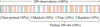 |
Fig. 1 Self-supervised masking strategy used for pretraining. For each light curve, 50% of the observation points are selected as the probed subset, which the model must predict. This subset consists of three components: 30% of the points are fully masked (hidden), 10% are replaced with random magnitudes, and 10% remain visible. This strategy forces the model to learn from context rather than simply memorizing positions. |
2.3 Probing and masking
The key to Astromer learning a good representation is to pretrain it to predict unseen observations along the light curve sequence. The probed subset consists of magnitudes designated for the model to predict. However, these values are excluded when calculating attention weights. We randomly select 50% of the total observations per window to constitute the probed subset. This subset is denoted by a binary mask vector, where 1 corresponds to the probed magnitude and zero otherwise.
In the self-attention mechanism, the attention weights for the probed subset are set to zero using masking. This design encourages the model to leverage the surrounding context to predict the probed magnitudes. During inference, however, masking is not applied. To prevent the model from over-relying on the masked observations during training, we adopted the following strategy. We assign 10% of visible observations and 10% of random observations in the probed subset. As a result, the actual masked portion is reduced to 30%, while the probed subset still corresponds to the initial 50%. This approach mitigates the risk of the model learning a direct identity mapping and improves its robustness to noise. In Fig. 1, we illustrate the composition of the final subsets, with the probed subset size fixed at 50% of the observations.
2.4 Encoder
The encoder comprises a sequence of attention blocks connected in series. The first block processes the input embeddings described in Sect. 2.2 and a binary mask matrix that specifies which observations to exclude from the attention mechanism. Subsequent blocks take as input the output of the preceding attention block as shown in Fig. 2.
Astromer 1 has two attention blocks, each containing four heads with 64 units. The outputs of the heads are concatenated, normalized, and combined through a fully connected layer, one hidden layer of 128 units, and a hyperbolic tangent activation.
Within each head, the attention values are computed from the similarity matrix derived using the query (Q), key (K), and value (V) matrices, normalized by the square root of dk = 256, the model’s embedding size. We note that Q, K, and V come from a linear transformation of the input embedding and have different values for each head and block.
![Mathematical equation: $\[\begin{aligned}\mathrm{Q} & =\mathrm{XW}_{query}^{\top}, \\\mathrm{K} & =\mathrm{XW}_{key}^{\top}, \quad \mathrm{V}=\mathrm{XW}_{value}^{\top}, \\\mathrm{W}_{att} & =\operatorname{Softmax}\left(\frac{\mathrm{QK}^{\top}-\infty \mathrm{M}}{\sqrt{d_k}}\right), \\\mathrm{Z} & =\mathrm{W}_{att} \mathrm{V}.\end{aligned}\]$](/articles/aa/full_html/2026/03/aa54026-25/aa54026-25-eq5.png) (3)
(3)
In Eq. (3), the mask matrix, M, prevents the masked subset of probed observations from contributing to the attention values. When M = 1, the argument of the softmax function is effectively negative infinity, resulting in a zero attention weight. In Astromer 1, the output of the last block serves as the final embedding. This matrix has two functions: reconstructing magnitudes during pretraining and serving as the embedding for downstream tasks.
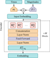 |
Fig. 2 Overview of the Astromer 1 architecture. An input embedding is formed by summing a positional encoding (PE) of the observation times and a linear projection of the magnitudes. This embedding is processed by an encoder composed of M=2 blocks, each containing H=4 self-attention heads, to produce the final light curve representation, which is derived from the output of the last block. |
2.5 Pretraining task
We pretrained the model to predict the magnitudes of the probed subset in each input sequence. This is achieved by passing the output embedding from the last attention block through a fully connected network with no hidden layers or activation. The result is a vector of estimated magnitudes, ![Mathematical equation: $\[\hat{\boldsymbol{x}} \in \mathbb{R}^{200 \times 1}\]$](/articles/aa/full_html/2026/03/aa54026-25/aa54026-25-eq6.png) , providing the reconstruction for each time point according to its related embedding.
, providing the reconstruction for each time point according to its related embedding.
We constrained the loss function to compute the root-mean-square error (RMSE) on the probed subset only, expressed as
![Mathematical equation: $\[\mathcal{L} o s s=\sqrt{\frac{1}{N-1} \sum_{i=0}^{N-1} \sum_{l=0}^{L-1} m_{i l}\left(x_{i l}-\hat{x}_{i l}\right)^2}.\]$](/articles/aa/full_html/2026/03/aa54026-25/aa54026-25-eq7.png) (4)
(4)
In Eq. (4), N represents the number of training samples, and L = 200 represents the length of the windows. Thus, the masking vector, mi, selectively includes errors from the probed subset.
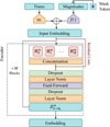 |
Fig. 3 Astromer 2 architecture, with an enhanced version of the model shown in Fig. 2. The primary architectural change is at the input stage: magnitudes designated for masking are now replaced by a single, trainable mask token. Additionally, the encoder’s depth is increased to M=6 blocks to improve its representational capacity. |
3 Astromer 2
Astromer 2 incorporates features that were not included in the initial version due to resource and time constraints. While Astromer 1 served as a proof of concept for generating effective embeddings, Astromer 2 builds on this foundation, introducing iterative enhancements to optimize performance at each stage.
Building upon the foundation of Astromer 1 discussed in Sect. 2, this section is dedicated solely to the enhancements that distinguish the principal features of Astromer 2. In Fig. 3, we show a visual representation of the updated architecture of Astromer 2.
3.1 Input embedding
The process for creating the input embedding for Astromer 2 remains the same as in the initial version. However, we replace the magnitudes targeted for masking with a trainable token that is zero-initialized and shared across all samples.
While the contribution of masked tokens is zero after the attention weight calculation, adding a mask token to replace the actual magnitude allows the model to recognize the tokens that are masked, which can be helpful during training. We also avoid potential information leaks that could arise from the all-to-all computation within the similarity matrix.
3.2 Encoder
The encoder of Astromer 2 has a significantly larger number of parameters, increasing from 661 505 to 3 953 409. This six-fold increase is due to the inclusion of six attention blocks, with each block containing four heads and 64 units. Additionally, we incorporated a dropout layer after the self-attention calculation, as depicted in Fig. 3.
3.3 Pretraining task
As with Astromer 1, we used the RMSE as the loss function. However, in Astromer 2, the losses are scaled based on observational uncertainties. These uncertainties are normalized to a range of 0 to 1 and their reciprocals are used as weights. Incorporating this scaling term into the error calculation enhances performance compared to Astromer 1,
![Mathematical equation: $\[\mathcal{L} o s s=\sqrt{\frac{1}{N-1} \sum_{i=0}^{N-1} \sum_{l=0}^{L-1} \frac{m_{i l}}{e_{i l}}\left(x_{i l}-\hat{x}_{i l}\right)^2}.\]$](/articles/aa/full_html/2026/03/aa54026-25/aa54026-25-eq8.png) (5)
(5)
In Eq. (5), eil ≠ 0 denotes the observation uncertainty associated with step, l, in window, i.
4 Data sources
In this section, we introduce our training data, including unlabeled light curves for pretraining and labeled samples for the downstream classification task.
4.1 Unlabeled data: MACHO
The MACHO project (Alcock et al. 1993) is aimed at detecting massive compact halo objects (MACHO labeled) to find evidence of dark matter in the Milky Way halo by searching for gravitational microlensing events. Light curves were collected from 1992 to 1999, producing light curves of more than a thousand observations (Alcock et al. 1999) in bands B and R. The observed sky was subdivided into 403 fields. Each field was constructed by observing a region of the sky or tile. The resulting data are available in a public repository1 which contains millions of light curves in bands B and R.
We selected a subset of fields 1, 101, 102, 103, and 104 containing 1 454 792 light curves for training. Similarly, we selected field 10 for testing, with a total of 74 594 light curves. MACHO observed in both bands simultaneously; therefore, having two magnitudes associated with each MJD. Since we are looking to improve on Astromer 2, we maintain the single band input. The light curves from this dataset that exhibited Gaussian noise characteristics were removed based on the criteria: |kurtosis| > 10, |skewness| > 1, and std >0.1. Additionally, we excluded observations with negative uncertainties (indicative of faulty measurements) or uncertainties greater than one (to maintain photometric quality). Outliers were also removed by discarding the 1st and 99th percentiles for each light curve. This additional filtering does not affect the total number of samples but reduces the number of observations when the criteria were applied.
4.2 Labeled data
To ensure a fair comparison with Astromer 1, we used the same sample selection from the MACHO (hereafter referred to as Alcock; Alcock et al. 2001) and the Asteroid Terrestrial-impact Last Alert System (hereafter referred to as ATLAS; Heinze et al. 2018) labeled catalogs. The former has a similar magnitude distribution, whereas the latter differs, as shown in Fig. 4.
The labeled classes in the MACHO dataset were produced through manual labeling supported by statistical analysis and feature extraction techniques, providing a curated and expert-classified dataset. For the ATLAS dataset, the labels are derived from automated classification pipelines based on template fitting and light curve features, which may introduce some uncertainty and biases inherent to automated labeling methods.
 |
Fig. 4 Magnitude distributions of the pretraining data (MACHO Labeled) and labeled sets (Alcock, ATLAS). The Alcock and MACHO distributions are similar, though Alcock is bimodal. The ATLAS data, from a different survey, shows a distinct distribution with higher variance. During training, all magnitudes are normalized, which removes the mean shifts shown here. |
Alcock catalog distribution.
4.2.1 Alcock
For the labeled data, we use the catalog of variable stars from Alcock et al. (2001), which contains labels for a subset of the MACHO light curves originating from 30 fields from the Large Magellanic Cloud. This labeled data will be used to train and evaluate the performance of the different embeddings on the classification task.
The selected data comprises 20894 light curves, which are categorized into six classes: Cepheid variables pulsating in the fundamental (Cep_0) and first overtone (Cep_1), eclipsing binaries (EC), long period variables (LPV), RR Lyrae ab and c (RRab and RRc, respectively). Table 1 summarizes the number of samples per class. We note that we used an updated version of the catalog, as described in Donoso-Oliva et al. (2023).
In Fig. 4, we compare the magnitude distributions between the Alcock and MACHO datasets. The former exhibits a bimodal distribution, which aligns with the fact that it represents a subset of the light curves from MACHO fields, while the latter encompasses light curves from only five fields. Similarly, we compared the distribution of time differences between consecutive observations (Δt). In Fig. 5, we show similar distributions, with comparable ranges and means of three and four days for MACHO and Alcock, respectively.
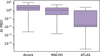 |
Fig. 5 Observation cadence (Δt, time between consecutive points) for the MACHO, Alcock, and ATLAS datasets. The boxplots show that MACHO and Alcock have similar, regular cadences (median ~3−4 days). The ATLAS dataset is distinct, with a much faster median cadence and greater variability in observation times. The y-axis uses a logarithmic scale to show the wide value range. |
ATLAS catalog distribution.
4.2.2 ATLAS
The Asteroid Terrestrial-impact Last Alert System (ATLAS; Tonry et al. 2018) is a survey developed by the University of Hawaii and funded by NASA. Operating since 2015, ATLAS has a global network telescopes, primarily focused on detecting asteroids and comets that could potentially threaten Earth. Observing in c (blue), o (orange), and t (red) filters. The variable star dataset used in this work was presented by Heinze et al. (2018) and includes 4.7 million candidate variable objects, included in the labeled and unclassified objects, as well as a dubious class. According to their estimates, this class is predominantly composed of 90% instrumental noise and only 10% genuine variable stars.
We analyzed 141 376 light curves from the ATLAS dataset, as detailed in Table 2. These observations, measured in the o passband, have a median cadence of ~15 minutes, which is significantly shorter than the typical cadence in the MACHO dataset. This substantial difference poses a challenge for the model, as it must adapt to such a distinct temporal distribution.
As done in Donoso-Oliva et al. (2023) to standardize the labels with other datasets, we combined the detached eclipsing binaries identified by full or half periods into the close binaries (CB) category and similarly merged detached binaries (DB). However, objects with labels derived from Fourier analysis were excluded, as these classifications do not directly align with astrophysical categories.
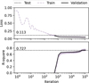 |
Fig. 6 Pretraining learning curves for Astromer 2, showing reconstruction loss (RMSE) versus training epochs. Both training (solid blue) and validation (orange) losses decrease and converge, indicating stable training. The final performance on the held-out test set is marked as a dotted line. |
4.3 MACHO versus ATLAS
Figures 4 and 5 illustrate the distributional differences between the unlabeled MACHO dataset and the labeled subsets discussed earlier. While the magnitudes show a notable shift between MACHO and ATLAS, our training strategy normalizes the light curves to a zero mean. As a result, the relationships between observations take precedence over the raw magnitude values. Consequently, we do not expect a substantial performance drop when transitioning between datasets. Heterogeneous cadences (Δt) present a significant challenge, as the model must extrapolate and account for fast variations to capture short-time information effectively. We demonstrate this in our first results from Astromer 2, where the F1 score on the ATLAS dataset is lower compared to MACHO when fewer labels are available for classification.
5 Results
The pretraining task of reconstructing the probed magnitudes is an essential component that allows the model to learn meaningful representations. Reconstructing probed magnitudes can be evaluated as a downstream regression task on labeled datasets, where the model’s ability to predict the magnitudes can be assessed. Here, we evaluate the potential of the representation in terms of regression.
Fig. 6 shows the learning curves from the pretraining of Astromer 2. The training took approximately 3 days using 4 A5000 GPUs. The model achieved an R2 of 0.732 with a root mean squared error (RMSE) of 0.113 on the probed subset. Astromer 1 had an RMSE of 0.148, making Astromer 2 0.035 better in terms of reconstruction error.
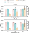 |
Fig. 7 Performance and computational cost comparison on test sets (three-fold cross-validation). The plots display the average performance in terms of RMSE (left y-axis) and training time in minutes (right y-axis) for the Alcock (left) and ATLAS (right) datasets, varying the number of samples per class (SPC). Red bars (pretrained) represent the pretrained model evaluated directly on the test set without fine-tuning. Turquoise bars (finetuned) show performance after fine-tuning with the indicated amount of data. Hatched beige bars indicate the fine-tuning time required. Error bars denote the range (minimum and maximum values) observed across the three folds. |
5.1 Downstream setup
Similar to Astromer 1, this work evaluates the embeddings across various scenarios, while controlling the number of samples per class (SPCs). When there are few SPCs, the quality of the embeddings becomes crucial, as they must capture fundamental features that enable the model to make predictions based solely on the shape of the light curves, without relying on additional information.
Using the labeled datasets, we construct three training scenarios with limited data by randomly sampling 20, 100, and 500 SPC to assess performance on downstream tasks. When the number of available labels is insufficient, sampling is performed with replacement. To account for variability in our experiments, we generate three folds for each scenario. To ensure fairness across scenarios, we evaluate all models on a shared three-fold test dataset consisting of 1000 SPC per fold. Hence, the models trained on 20, 100, and 500 SPC were evaluated against this common dataset.
In the initial stage of the downstream pipeline, we performed the finetuning. This involves loading the pretrained weights and adapting the encoder parameters to the target domain. Finetuning follows the same pretraining setup, predicting a random probed subset containing 50% of the magnitudes per sequence.
5.2 Finetuning
In Fig. 7, we present the RMSE results for each scenario. The reported values are calculated across the total number of observations without masking, allowing for a fair comparison as the error could be biased by the random masking selection.
As shown in Fig. 7, finetuning the model on the Alcock dataset does not result in significant improvements, indicating that the pretrained model already captures most of the relevant information, despite the out-of-distribution modality discussed in Sect. 4.3. In contrast, finetuning on ATLAS leads to a notable improvement. Specifically, with 100 SPC, we observe a 23% reduction in RMSE compared to the pretrained model. However, the performance improvement between 100 and 500 SPC is minimal, with only small variations.
The most computationally intensive scenario takes approximately three minutes to finetune, which is significantly faster than the days required for pretraining. While the time for MACHO increases with more samples, in ATLAS, we observe almost no variation between 20 and 100 SPC. This is because MACHO samples are longer than ATLAS samples, resulting in a more substantial increase in the number of windows as the number of SPC grows. This explains the more significant rise in computing time when going from 20 to 100 MACHO SPC.
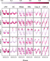 |
Fig. 8 Visualization of attention weights from the first encoder block on sample light curves from the Alcock dataset. Each of the first eight plots shows the average attention from one head (colored bar, top), with the final plot showing the mean across all heads. The light curves are folded by their period for clarity. The model consistently focuses attention on points of maximum and minimum brightness. |
5.3 Visualizing reconstruction
Figures 8 and 9 show the mean attention weights from each attention head, along with the mean across all heads, for sample light curves from the Alcock and ATLAS datasets, respectively. For each dataset, we present one representative example for each class to illustrate the model’s focus. For visualization purposes, the light curves were folded by their period; however, Astromer does not receive folded inputs during processing. We display the attention from the first attention block, as its interpretation is more intuitive compared to intermediate layers, where attention is computed over more abstract embeddings. As shown in both figures, each attention head learns to focus on different parts of the sequence. Notably, there is a consistent pattern where attention is most strongly concentrated at points of maximum and minimum brightness, suggesting that these have been identified as key features for reconstruction and characterization. This demonstrates a consistent feature-learning strategy across different datasets and variable star types.
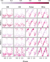 |
Fig. 9 Same as Fig. 8, but for sample light curves from the ATLAS dataset. The model again learns to focus on the extrema of the light curves, demonstrating a consistent feature-learning strategy across different datasets. |
5.4 Classification
Evaluating classification performance is crucial for assessing the overall effectiveness of Astromer, as it serves as a common benchmark for evaluating the quality of embeddings. After finetuning on labeled subsets of 20, 100, and 500 SPCs, the encoder is frozen, meaning its weights are no longer updated.
Astromer is used to extract the representation, which is fed to another classifier model. The same labeled data are used to train a classifier. In this setup, only the classifier section receives label-based gradients, while the encoder focuses exclusively on capturing dependencies between observations.
Per-sample embeddings were generated by averaging the attention vectors from the encoder, with trainable parameters γ0, ..., γm weighting the outputs of each block. The resulting embedding is then passed through a multilayer perceptron (MLP) consisting of three hidden layers with 1024, 512, and 256 units, respectively, each using ReLU activation. A fully connected layer without activation predicts the final label, as shown in Fig. 10.
Fig. 11 presents the F1 scores for the Alcock dataset across different scenarios. We focus our analysis on the improvements over our previous model, rather than re-evaluating against classical models, as this benchmark was already established in our initial work (Donoso-Oliva et al. 2023). For a direct comparison, the figure includes the F1 scores from Astromer 1, using both weighted per-sample embeddings (A1) and unweighted embeddings (A2) as detailed in our previous paper.
The improvements are most pronounced when evaluating classification performance on the ATLAS dataset. As depicted in Fig. 12, the new version of Astromer exhibits a significant advantage in generalizing to other datasets. With just 20 SPC, Astromer achieves a F1-score improvement of over 15%. Thus, Astromer’s performance with 20 SPC surpasses the results previously reported 500 SPC.
Weighted per-sample embeddings play a critical role by allowing the model to use intermediate representations instead of depending exclusively on the final one. During pretraining, the encoder focuses on reconstructing magnitudes from the last embedding, which could result in representations tailored to the reconstruction task rather than optimized for discrimination.
To examine the role of intermediate embeddings, we plot the gamma parameters after training the classifier on both the Alcock and ATLAS datasets. As shown in Fig. 13, the weights assigned to intermediate embeddings are higher than those for the initial or final ones. This disparity becomes more pronounced as the number of training samples increases.
Figs. 14 and 15 present t-SNE projections of the test set embeddings, derived from the output of each attention block for the first data fold. Unlike standard text-based BERT models, our architecture does not employ a [CLS] token to obtain a summary representation of the sequence. Therefore, an aggregation step is necessary to produce a single vector for each time series. To achieve this, we reduce the (200, 256) output tensor from each block by averaging across the 200 time steps, resulting in a representative (1, 256) vector.
This averaging strategy was selected over other alternatives, such as concatenation and the maximum, as it consistently produces more coherent clusters for visualization. A detailed quantitative justification supporting this decision is provided in the Appendix A.
The first thing to notice is that there is evidence that Astromer properly separates classes in both the Alcock and ATLAS datasets. We recall that these embeddings were trained solely on light curve reconstruction, without any information about the labels.
A key advantage of our self-supervised approach is its ability to enable object retrieval and similarity searches directly in the embedding space without requiring labeled data. As shown in Figs. 14 and 15, the model organizes light curves with similar characteristics close to one another, which facilitates effective clustering and retrieval. This capability is particularly valuable in astronomical datasets where labeling is costly and incomplete, providing a powerful tool for exploratory data analysis and discovery beyond classification tasks.
Classes are separated in different ways depending on the block. For both Alcock and ATLAS, the first block does not seem to separate classes at all, while other blocks exhibit better discrimination. This aligns with the γ parameters we introduced to weight each block’s output during classifier training (see Fig. 13).
Alternatively, we can observe the effect of class separation in the confusion matrices in Figs. 16 and 17. Specifically, for the Alcock dataset, the main confusion occurs between RR Lyrae types ab and c. A similar pattern is observed in the projection of Fig. 14, where the RRab and RRc points are mixed together. In ATLAS, there is another class, which can be particularly confusing for the model. As observed in Fig. 15, the points corresponding to the other class are sparsely distributed in the embedding space.
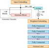 |
Fig. 10 Downstream classification head architecture. A weighted-average embedding from the Astromer encoder is passed through a feed-forward network (FFN) with three hidden layers to produce the final class prediction. Only the weights of this classifier head are trained on the labeled data. |
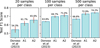 |
Fig. 11 Classification performance (F1-score) on the Alcock (MACHO Labeled) dataset. The plot compares Astromer 2 (A2) against Astromer 1 (A1) and the published results from Donoso-Oliva et al. (2023) across scenarios with 20, 100, and 500 labeled samples per class (SPC). Astromer 2 consistently outperforms previous versions, especially in low-data regimes. |
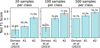 |
Fig. 12 Same as Fig. 11, but for the ATLAS dataset. The performance improvement of Astromer 2 is even more pronounced on this out-of-distribution dataset, where it significantly surpasses all previous results, even when trained with only 20 SPC. |
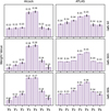 |
Fig. 13 Learned gamma (γ) weights for the weighted-average embedding. Each γi scales the contribution of the output from block i of the encoder (γ0 for the input). The classifier learns to assign higher importance to intermediate layers (2−5) rather than the initial or final layers, especially as more training data becomes available. |
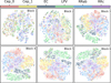 |
Fig. 14 t-SNE visualization of embeddings from each of the six encoder blocks for the Alcock (MACHO Labeled) test set. Each point is a light curve, colored by its true class. The plots show that class structure emerges and improves in the intermediate and deeper layers, even though the model was pretrained without any label information. |
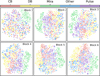 |
Fig. 15 Same as Fig. 14, but for the ATLAS test set embeddings. A similar trend is observed where embeddings from deeper layers provide better class separation, demonstrating the model’s ability to learn meaningful structures for different data distributions. |
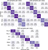 |
Fig. 16 Confusion matrices for classification on the Alcock test set, for models trained with 20, 100, and 500 samples per class (SPC). As more labeled data are used, the diagonal (correct classifications) becomes stronger. The most persistent confusion occurs between the RR Lyrae subtypes (RRab and RRc). |
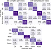 |
Fig. 17 Same as Fig. 16, but for the ATLAS test set. Performance improves with more SPC, but significant confusion remains involving the other class, which is inherently diverse and overlaps with defined classes in the feature space. |
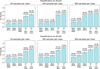 |
Fig. 18 Ablation study comparison. Classification performance (mean F1-score) on the MACHO labeled (top) and ATLAS (bottom) datasets across different training sizes (20, 100, and 500 samples per class). The study compares baseline architectures (MLP, GRU, Raw RNN) against the proposed Astromer 2 encoder (A2) equipped with different aggregation strategies: max pooling vs. skip connection. Error bars and values indicate the standard deviation over multiple runs. |
5.5 Ablation study
To rigorously assess the contribution of the proposed Astromer architecture, we conducted an ablation study comparing our method against three distinct baselines. These comparisons were designed to disentangle the benefits provided by the input representation (embedding) from those provided by the transformer-based encoder. The baselines are defined as follows:
Baseline raw: this model processes the raw input sequence (magnitudes and time) directly using a gated recurrent unit (GRU). It does not utilize the positional encoding or the magnitude projection introduced in this work. This setup mimics the baseline approach used in Donoso-Oliva et al. (2023) (Astromer 1), serving as a standard reference for recurrent neural networks operating on irregular time series without specialized embeddings;
Baseline MLP: this model utilizes the full Astromer input embedding layer (Sect. 3.1) to project magnitudes and encode time positions. However, instead of a temporal encoder (transformer or RNN), it applies a masked average pooling operation immediately after the embedding step, followed by an MLP classifier. This baseline tests the effectiveness of the input transformation alone, determining how much performance can be gained simply by properly encoding time and magnitude before aggregation;
Supervised GRU: this model also utilizes the Astromer input embedding layer but processes the sequence using a GRU instead of the transformer encoder. This serves as a robust baseline that benefits from the same initial feature engineering as Astromer, thereby isolating the performance difference between a recurrent architecture and the self-attention mechanism.
Furthermore, to validate the aggregation strategy used in our downstream classification head, we compared our proposed skip-connection weighted average (Sect. 5.4) against a standard max pooling strategy. In this setup, the max pooling variant reduces the sequence of embeddings from the final encoder layer into a single vector by computing the maximum value across the temporal dimension, discarding the hierarchical information from intermediate layers.
Figure 18 summarizes the F1-scores for these experiments. The most prominent result is the substantial impact of the Astromer input embedding on model performance. Regardless of whether the subsequent encoder is a GRU or a transformer, models equipped with our specialized magnitude projection and positional encoding consistently outperform the raw RNN baseline. This confirms that explicitly modeling the temporal geometry of the light curves via sinusoidal embeddings is far superior to feeding raw time intervals, providing a richer feature space that enhances the learning capability of any downstream architecture.
Crucially, the superiority of the Astromer embeddings is most decisive in data-scarce scenarios. In the 20 SPC experiment, the raw RNN fails to capture robust decision boundaries, displaying a significantly lower level of performance. In contrast, simply adopting the Astromer embedding (as seen in the supervised GRU and transformer variants) drastically improves the F1-score, enabling the models to generalize effectively even with very few examples. While the transformer encoder with skip-connections achieves the highest overall peak, this ablation demonstrates that the robustness in low-data regimes is fundamentally driven by our proposed input representation strategy, which effectively lowers the sample complexity required for convergence compared to raw inputs.
6 Conclusion
This paper presents the updated version of Astromer, a self-supervised model designed to extract general-purpose embeddings from light curve data. We demonstrate that Astromer 2 outperforms its predecessor, Astromer 1, across multiple scenarios, including both the Alcock and ATLAS datasets. The key improvements in classification performance, especially when trained with limited labeled samples, highlight the informative power of the embeddings in discriminating between different classes.
The results show that Astromer 2 achieves significant gains in F1 score, especially with small training sets, underscoring the effectiveness of the weighted per-sample embeddings and the model’s ability to generalize across different datasets. The analysis of attention weights further reveals that intermediate embeddings contribute meaningfully to the model’s performance, focusing more on certain parts of the input data during the classification task.
These findings confirm the potential of Astromer as a robust tool for light curve analysis, showing that self-supervised learning can provide valuable insights into astronomical data. Future works on Astromer will focus on incorporating multi-band data, either as an additional feature embedding or by directly constraining the embedding space. Additionally, we plan to train Astromer on the entire survey, bringing in more data during pretraining and potentially capturing more informative representations.
Data availability
The source code, model weights, and experimental results are available in our official GitHub organization: https://github.com/astromer-science. General information and practical documentation can be found on our website: https://www.stellardnn.org/projects/astromer/index.html. Supplementary materials, including the light curve reconstruction figures for Appendix B and the foundational model weights, are permanently archived on Zenodo at https://doi.org/10.5281/zenodo.18207945.
Acknowledgements
The authors acknowledge support from the National Agency for Research and Development (ANID) grants: FONDECYT Regular 1231877 (C.D.O., G.C.V., M.C.L., D.M.C.). G.C.V. acknowledges support from the Millennium Science Initiative through the Millennium Institute of Astrophysics (MAS) AIM23-0001. C.D.O. acknowledges support from the Millennium Nucleus on Young Exoplanets and their Moons (YEMS) through the Millennium Science Initiative Program (NCN2024_001). This work was also supported by the Center for Data and Artificial Intelligence at the Universidad de Concepción. We thank the MACHO and ATLAS collaborations for making their data publicly available. This research has made use of the VizieR catalogue access tool, CDS, Strasbourg, France.
References
- Alcock, C., Akerlof, C. W., Allsman, R. A., et al. 1993, Nature, 365, 621 [NASA ADS] [CrossRef] [Google Scholar]
- Alcock, C., Allsman, R. A., Alves, D. R., et al. 1999, PASP, 111, 1539 [NASA ADS] [CrossRef] [Google Scholar]
- Alcock, C., Allsman, R., Alves, D. R., et al. 2001, ApJ, 554, 298 [NASA ADS] [CrossRef] [Google Scholar]
- Awais, M., Naseer, M., Khan, S., et al. 2025, IEEE Trans. Pattern Anal. Mach. Intell., 47, 2245 [Google Scholar]
- Bommasani, R., Hudson, D. A., Adeli, E., et al. 2021, arXiv preprint [arXiv:2108.07258], Stanford HAI White Paper [Google Scholar]
- Chaini, S., Mahabal, A., Kembhavi, A., & Bianco, F. B. 2024, Astron. Comput., 48, 100850 [Google Scholar]
- Deb, S., & Singh, H. P. 2009, A&A, 507, 1729 [NASA ADS] [CrossRef] [EDP Sciences] [Google Scholar]
- Debosscher, J., Sarro, L. M., Aerts, C., et al. 2007, A&A, 475, 1159 [NASA ADS] [CrossRef] [EDP Sciences] [Google Scholar]
- Devlin, J., Chang, M.-W., Lee, K., & Toutanova, K. 2019, in Proceedings of the 2019 Conference of the North American Chapter of the Association for Computational Linguistics, 4171 [Google Scholar]
- Donoso-Oliva, C., Becker, I., Protopapas, P., et al. 2023, A&A, 670, A54 [NASA ADS] [CrossRef] [EDP Sciences] [Google Scholar]
- Heinze, A. N., Tonry, J. L., Denneau, L., et al. 2018, AJ, 156, 241 [Google Scholar]
- Lanusse, F., Parker, L., Golkar, S., et al. 2023, in NeurIPS 2023 AI for Science Workshop [Google Scholar]
- Liang, Y., Wen, H., Nie, Y., et al. 2024, in Proceedings of the 30th ACM SIGKDD Conference on Knowledge Discovery and Data Mining, 6555 [Google Scholar]
- Martínez-Galarza, J. R., Bianco, F. B., Crake, D., et al. 2021, MNRAS, 508, 5734 [CrossRef] [Google Scholar]
- Nun, I., Protopapas, P., Sim, B., et al. 2015, A&A, 583, A55 [NASA ADS] [CrossRef] [EDP Sciences] [Google Scholar]
- Pantoja, R., Catelan, M., Pichara, K., & Protopapas, P. 2022, MNRAS, 517, 3660 [Google Scholar]
- Parker, L., Lanusse, F., Golkar, S., et al. 2024, MNRAS, 531, 4990 [Google Scholar]
- Richards, J. W., Starr, D. L., et al. 2011, ApJ, 733, 10 [NASA ADS] [CrossRef] [Google Scholar]
- Rizhko, M., & Bloom, J. S. 2024, in NeurIPS 2024 Workshop Foundation Models for Science [Google Scholar]
- Sánchez-Sáez, P., Reyes, I., Valenzuela, C., et al. 2021, AJ, 161, 141 [CrossRef] [Google Scholar]
- Tonry, J. L., Denneau, L., Heinze, A. N., et al. 2018, PASP, 130, 064505 [Google Scholar]
- Wang, J., Jiang, H., Liu, Y., et al. 2025, Inform. Fusion, 115, 102710 [Google Scholar]
R2 (coefficient of determination) measures the proportion of variance in the observed data explained by the model. It ranges from −∞ to 1, with 1 indicating perfect prediction.
Appendix A Embedding visualization method
To select an optimal method for visualizing the class-based clustering of our pretrained encoder embeddings, we conducted a quantitative comparison of three distinct aggregation strategies. The methods evaluated were: averaging the token embeddings across the time dimension, concatenating all token embeddings, and applying max pooling across the time dimension.
We used the silhouette score with a cosine metric as the evaluation criterion to determine which method produced the most coherent and well-separated clusters. The score for each method was calculated at the output of each of the six attention blocks in the encoder.
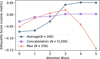 |
Fig. A.1 Silhouette score, calculated with a cosine metric, as a function of the attention block number for three embedding aggregation methods. The methods compared are averaging (blue circles), concatenation (purple squares), and max pooling (red triangles). The averaging method consistently achieves the highest score in the final layers, indicating it is the most suitable strategy for producing coherent visualizations of class clusters. |
The results of this analysis are presented in Fig. A.1. The key findings from this comparison are:
The averaging method consistently achieves the highest silhouette score in the later, more specialized layers of the encoder (blocks 3, 4, and 5), peaking at a score above 0.05. This indicates that averaging produces the most distinct visual clusters.
The max pooling method shows competitive performance in the middle layers but degrades sharply in the final blocks, suggesting it does not capture the final, refined embedding structure as effectively.
The concatenation method results in a score of approximately zero across all blocks, implying it does not produce a useful clustering structure for visualization.
Based on this evidence, we selected the averaging strategy for all embedding visualizations presented in this work.
Appendix B Examples of masked value reconstruction
To provide a qualitative assessment of the model’s ability to learn the underlying structure of the light curves, we present examples of its reconstruction performance on masked input data.
The analysis covers a selection of variable star classes: Cepheid (Cep 0, Cep 1), RR Lyrae (RRab, RRc), eclipsing binary (EC), and long period variable (LPV). For each class, the reconstruction is analyzed through three different views:
Time series reconstruction: This view displays the original light curve in the time domain, showing unmasked observations, the true values of masked points, and the model predictions.
Prediction versus true: A direct comparison of predicted versus true magnitudes for the masked data points, including the root mean square error (RMSE).
Folded reconstruction: The reconstruction of masked points in phase space, with the light curve folded by its dominant period to assess how the model captures periodic variability.
Detailed figures showing these reconstructions for each class have been moved to the Zenodo repository to streamline the paper layout, as specified in the data availability section.
All Tables
All Figures
|
Fig. 1 Self-supervised masking strategy used for pretraining. For each light curve, 50% of the observation points are selected as the probed subset, which the model must predict. This subset consists of three components: 30% of the points are fully masked (hidden), 10% are replaced with random magnitudes, and 10% remain visible. This strategy forces the model to learn from context rather than simply memorizing positions. |
| In the text | |
|
Fig. 2 Overview of the Astromer 1 architecture. An input embedding is formed by summing a positional encoding (PE) of the observation times and a linear projection of the magnitudes. This embedding is processed by an encoder composed of M=2 blocks, each containing H=4 self-attention heads, to produce the final light curve representation, which is derived from the output of the last block. |
| In the text | |
|
Fig. 3 Astromer 2 architecture, with an enhanced version of the model shown in Fig. 2. The primary architectural change is at the input stage: magnitudes designated for masking are now replaced by a single, trainable mask token. Additionally, the encoder’s depth is increased to M=6 blocks to improve its representational capacity. |
| In the text | |
|
Fig. 4 Magnitude distributions of the pretraining data (MACHO Labeled) and labeled sets (Alcock, ATLAS). The Alcock and MACHO distributions are similar, though Alcock is bimodal. The ATLAS data, from a different survey, shows a distinct distribution with higher variance. During training, all magnitudes are normalized, which removes the mean shifts shown here. |
| In the text | |
|
Fig. 5 Observation cadence (Δt, time between consecutive points) for the MACHO, Alcock, and ATLAS datasets. The boxplots show that MACHO and Alcock have similar, regular cadences (median ~3−4 days). The ATLAS dataset is distinct, with a much faster median cadence and greater variability in observation times. The y-axis uses a logarithmic scale to show the wide value range. |
| In the text | |
|
Fig. 6 Pretraining learning curves for Astromer 2, showing reconstruction loss (RMSE) versus training epochs. Both training (solid blue) and validation (orange) losses decrease and converge, indicating stable training. The final performance on the held-out test set is marked as a dotted line. |
| In the text | |
|
Fig. 7 Performance and computational cost comparison on test sets (three-fold cross-validation). The plots display the average performance in terms of RMSE (left y-axis) and training time in minutes (right y-axis) for the Alcock (left) and ATLAS (right) datasets, varying the number of samples per class (SPC). Red bars (pretrained) represent the pretrained model evaluated directly on the test set without fine-tuning. Turquoise bars (finetuned) show performance after fine-tuning with the indicated amount of data. Hatched beige bars indicate the fine-tuning time required. Error bars denote the range (minimum and maximum values) observed across the three folds. |
| In the text | |
|
Fig. 8 Visualization of attention weights from the first encoder block on sample light curves from the Alcock dataset. Each of the first eight plots shows the average attention from one head (colored bar, top), with the final plot showing the mean across all heads. The light curves are folded by their period for clarity. The model consistently focuses attention on points of maximum and minimum brightness. |
| In the text | |
|
Fig. 9 Same as Fig. 8, but for sample light curves from the ATLAS dataset. The model again learns to focus on the extrema of the light curves, demonstrating a consistent feature-learning strategy across different datasets. |
| In the text | |
|
Fig. 10 Downstream classification head architecture. A weighted-average embedding from the Astromer encoder is passed through a feed-forward network (FFN) with three hidden layers to produce the final class prediction. Only the weights of this classifier head are trained on the labeled data. |
| In the text | |
|
Fig. 11 Classification performance (F1-score) on the Alcock (MACHO Labeled) dataset. The plot compares Astromer 2 (A2) against Astromer 1 (A1) and the published results from Donoso-Oliva et al. (2023) across scenarios with 20, 100, and 500 labeled samples per class (SPC). Astromer 2 consistently outperforms previous versions, especially in low-data regimes. |
| In the text | |
|
Fig. 12 Same as Fig. 11, but for the ATLAS dataset. The performance improvement of Astromer 2 is even more pronounced on this out-of-distribution dataset, where it significantly surpasses all previous results, even when trained with only 20 SPC. |
| In the text | |
|
Fig. 13 Learned gamma (γ) weights for the weighted-average embedding. Each γi scales the contribution of the output from block i of the encoder (γ0 for the input). The classifier learns to assign higher importance to intermediate layers (2−5) rather than the initial or final layers, especially as more training data becomes available. |
| In the text | |
|
Fig. 14 t-SNE visualization of embeddings from each of the six encoder blocks for the Alcock (MACHO Labeled) test set. Each point is a light curve, colored by its true class. The plots show that class structure emerges and improves in the intermediate and deeper layers, even though the model was pretrained without any label information. |
| In the text | |
|
Fig. 15 Same as Fig. 14, but for the ATLAS test set embeddings. A similar trend is observed where embeddings from deeper layers provide better class separation, demonstrating the model’s ability to learn meaningful structures for different data distributions. |
| In the text | |
|
Fig. 16 Confusion matrices for classification on the Alcock test set, for models trained with 20, 100, and 500 samples per class (SPC). As more labeled data are used, the diagonal (correct classifications) becomes stronger. The most persistent confusion occurs between the RR Lyrae subtypes (RRab and RRc). |
| In the text | |
|
Fig. 17 Same as Fig. 16, but for the ATLAS test set. Performance improves with more SPC, but significant confusion remains involving the other class, which is inherently diverse and overlaps with defined classes in the feature space. |
| In the text | |
|
Fig. 18 Ablation study comparison. Classification performance (mean F1-score) on the MACHO labeled (top) and ATLAS (bottom) datasets across different training sizes (20, 100, and 500 samples per class). The study compares baseline architectures (MLP, GRU, Raw RNN) against the proposed Astromer 2 encoder (A2) equipped with different aggregation strategies: max pooling vs. skip connection. Error bars and values indicate the standard deviation over multiple runs. |
| In the text | |
|
Fig. A.1 Silhouette score, calculated with a cosine metric, as a function of the attention block number for three embedding aggregation methods. The methods compared are averaging (blue circles), concatenation (purple squares), and max pooling (red triangles). The averaging method consistently achieves the highest score in the final layers, indicating it is the most suitable strategy for producing coherent visualizations of class clusters. |
| In the text | |
Current usage metrics show cumulative count of Article Views (full-text article views including HTML views, PDF and ePub downloads, according to the available data) and Abstracts Views on Vision4Press platform.
Data correspond to usage on the plateform after 2015. The current usage metrics is available 48-96 hours after online publication and is updated daily on week days.
Initial download of the metrics may take a while.