| Issue |
A&A
Volume 707, March 2026
|
|
|---|---|---|
| Article Number | A259 | |
| Number of page(s) | 18 | |
| Section | Extragalactic astronomy | |
| DOI | https://doi.org/10.1051/0004-6361/202556109 | |
| Published online | 09 March 2026 | |
The dynamical lineage of ultra-diffuse galaxies from TNG50-1
Indian Institute of Science Education and Research Tirupati 517619, India
★ Corresponding authors: This email address is being protected from spambots. You need JavaScript enabled to view it.
, This email address is being protected from spambots. You need JavaScript enabled to view it.
Received:
26
June
2025
Accepted:
12
December
2025
Abstract
Context. The formation and evolution of ultra-diffuse galaxies (UDGs) continue to be a puzzle. Broadly, the formation scenarios of UDGs can be classified into two categories: a massive yet failed L*-type and a dwarf-like origin. The similarities and differences in the morphological and kinematical properties of the UDGs with their possible precursors may provide important constraints on their origin and evolutionary history.
Aims. We compared and contrasted structural, orbital, and kinematical properties of the UDGs with other galaxy populations, namely, low-surface brightness galaxies (LSBs), L*-type or high-surface brightness galaxies (HSBs), and the dwarf galaxies.
Methods. We selected a sample of UDG, LSB, HSB, and dwarf galaxies from the TNG50-1 box of the IllustrisTNG simulation. We first obtained a few possible scaling relations involving their mass properties and conducted Spearman’s rank correlation tests to analyse if the regression fits for UDGs are in compliance with those of the other galaxy samples. Then, we studied the cut-outs of the individual galaxies to investigate the intrinsic shapes of their dark matter (DM) and stellar components. We also investigated their orbital and kinematical properties by evaluating a few parameters composed of velocity dispersion components. Finally, we constructed mock integral field spectroscopic data using the publicly available software SimSpin to extract the kinematic moment maps of the line-of-sight velocity distribution and probe the stellar kinematic properties of our galaxy samples. In all the cases, we divided the samples in two subpopulations: isolated and tidally bound to study the effect of the local environment.
Results. We observed that the UDGs and the dwarf galaxies have nearly similar regression fits in the following parameter spaces: (a) stellar-to-gas mass ratio versus gas mass, (b) stellar-to-gas mass ratio versus total dynamical mass, and (c) total baryonic mass versus total dynamical mass. Further, we can infer that the isolated UDGs can be classified as prolate, while the tidally bound UDGs can exhibit both prolate and oblate shapes. The DM and stellar velocity anisotropy of the UDGs suggest that they reside in a cored low-mass halo and can be classified as early-type galaxies. Finally, their stellar kinematic properties suggest that the UDGs are slow-rotators exhibiting low to nearly no rotation.
Conclusions. The UDGs and the dwarf galaxies share similarities as far as the aforementioned possible scaling relations are concerned. Both the isolated UDGs and dwarf population can be characterised by prolate shapes, unlike other galaxy populations. However, the tidally bound UDGs exhibit both prolate as well as oblate shapes. The velocity anisotropy of the UDGs and the dwarfs hint at the fact that they may have originated in a dwarf-like halo, as opposed to the LSBs or the HSBs. Moreover, the UDGs and the dwarfs can be classified as early-type slow-rotating galaxies, in contrast to the late-type, disc-dominated, and fast-rotating LSBs and the HSBs. Therefore, we conclude that the UDGs and the dwarfs possibly have a common dynamical lineage.
Key words: galaxies: dwarf / galaxies: evolution / galaxies: formation / galaxies: halos / galaxies: kinematics and dynamics / galaxies: structure
© The Authors 2026
 Open Access article, published by EDP Sciences, under the terms of the Creative Commons Attribution License (https://creativecommons.org/licenses/by/4.0), which permits unrestricted use, distribution, and reproduction in any medium, provided the original work is properly cited.
This article is published in open access under the Subscribe to Open model. This email address is being protected from spambots. You need JavaScript enabled to view it. to support open access publication.
1. Introduction
Ultra-diffuse galaxies (UDGs) have attracted considerable attention since their discovery in the Coma cluster and then subsequently in almost all cosmological environments in the nearby Universe due to their remarkably faint yet extended appearance (van Dokkum et al. 2015a,b; Koda et al. 2015; Mihos et al. 2015; Muñoz et al. 2015; Yagi et al. 2016; Martínez-Delgado et al. 2016; van der Burg et al. 2017; Román & Trujillo 2017; Venhola et al. 2017; Janssens et al. 2017, 2019; Müller et al. 2018; Forbes et al. 2019; Prole et al. 2021; Zaritsky et al. 2019; Román et al. 2019; Barbosa et al. 2020). In fact, UDGs are defined as galaxies with a g-band central surface brightness of μg, 0 > 24 mag arcsec−2 and effective radii of Re > 1.5 kpc. In general, UDGs are dark matter (DM) dominated (Di Cintio et al. 2017; Toloba et al. 2018; van Dokkum et al. 2019; Forbes et al. 2021; Gannon et al. 2021; Kong et al. 2022; Benavides et al. 2023). Nevertheless, there exist some UDGs that are reportedly DM-free (Mancera Piña et al. 2022; van Dokkum et al. 2022). The diversity in DM content in these galaxies makes them ideal testing beds to constrain models of formation and evolution of galaxies in different cosmological paradigms.
A variety of physical mechanisms have been proposed in the literature to explain the formation and evolution of UDGs. Since UDGs consist of older stellar populations, they are primarily understood to originate from ‘failed’ L*-type galaxies that ceased star formation after gas loss driven by ram pressure stripping or harassment (van Dokkum et al. 2015a,b; Peng & Lim 2016; Toloba et al. 2018; Janssens et al. 2022). Alternatively, UDGs are believed to be formed from dwarf galaxies via transformation through several intrinsic or/and extrinsic physical mechanisms, such as (1) formation in dwarf-like yet high-spin DM halos (Amorisco & Loeb 2016); (2) expansion of DM and stellar halos due to feedback-driven gas outflows (Di Cintio et al. 2017); (3) mass loss or mass redistribution due to the group and cluster tidal field (Jiang et al. 2019; Carleton et al. 2019; Tremmel et al. 2020); (4) accretion or infall into a cluster environment (Sales et al. 2020); (5) origination in backsplash orbits (Benavides et al. 2021); (6) fall-outs of early mergers (Wright et al. 2021); and (7) redistribution of a fraction of star-forming gas to the outer region while undergoing galactic fountain, therefore triggering star-formation at extended radii (Zheng et al. 2025). Interestingly, while the alternative formation scenarios appear to be more viable, they can hardly explain the presence of a surprisingly greater number of globular clusters (GCs) in some UDGs (Toloba et al. 2023; Haacke et al. 2025). Moreover, recent studies have substantiated the validity of both the contrasting formation scenarios based on the number of GCs found in the UDGs (Forbes et al. 2020; Buzzo et al. 2022, 2024). Clearly, a general agreement is still lacking in the literature involving the formation of the UDGs.
To identify the fundamental formation mechanism of the UDGs, several observational and simulation studies have probed their intrinsic stellar morphology, which emerged as another subject of debate. While the Coma UDGs were observed to exhibit prolate morphologies (Burkert 2017), an extensive sample of UDGs, including the ones existing in the field as well as those located in several low-to-intermediate redshift galaxy clusters, exhibit stellar shapes that are well described by an oblate-triaxial model (Rong et al. 2020; Kado-Fong et al. 2021). On the other hand, the field UDGs found in the idealised zoom-in simulations were observed to display both prolate as well as oblate shapes (Jiang et al. 2019; Cardona-Barrero et al. 2020). In parallel, some studies have suggested that the UDGs display oblate shapes when they are in the field and prolate when in denser environments (Liao et al. 2019; Van Nest et al. 2022), while still other studies have reported no significant difference between the cluster and field UDGs as far as their intrinsic shapes are concerned (Kadowaki et al. 2021; Benavides et al. 2023). Although the intrinsic shapes of the DM halo may impact the stellar orbital distribution by modifying the underlying halo potential, this aspect has not received much attention in the literature in the context of UDGs. Furthermore, the stellar orbital and kinematic features may impose important constraints on the formation and evolutionary history of these galaxies. A number of field and cluster UDGs show lower circular velocities or nearly no significant rotation, while some of the cluster UDGs exhibit major, intermediate, or minor axis rotation (Leisman et al. 2017; Mancera Piña et al. 2019; Sengupta et al. 2019; Chilingarian et al. 2019). The integral field spectroscopic (IFS) observations of some cluster UDGs suggest the presence of both rotating (including NGC1052-DF2) and non-rotating (including DF44) UDGs (Emsellem et al. 2019; van Dokkum et al. 2019; Iodice et al. 2023; Buttitta et al. 2025). Similarly, based on analysis of the synthetic 2D stellar kinematic map of the field UDGs in the NIHAO zoom-in simulation, both rotation- and dispersion-supported UDGs have been observed to be present in the isolated environment with nearly equal probability (Cardona-Barrero et al. 2020). In fact, the higher-order Gauss-Hermite (GH) moments of the line-of-sight velocity distribution (LOSVD) extracted from the IFS data may describe the stellar kinematic properties of these galaxies in greater detail (van der Marel & Franx 1993; Gerhard 1993). However, due to their faintness, the observations require a longer exposure time to achieve a significant signal-to-noise ratio for a robust GH parametrisation. To date, DF44 is the only UDG for which the higher-order GH coefficients were derived from the IFS data gathered via a series of VLT/MUSE IFS observations over a span of a few months, amounting to an overall exposure time of 25.3 h (van Dokkum et al. 2019). One way to overcome this limitation is by simulating the mock IFS spectra of the UDGs by using galaxy cut-outs from state-of-the-art large-scale cosmological simulations as initial conditions. This will also help in studying and analysing a larger sample of galaxies, which is necessary from a statistical viewpoint to identify the possible trends, if any, present in their structural and morphological properties.
In our previous study, we observed that the isolated HI-rich UDGs and the dwarf irregular galaxies share similarities in their structural and kinematic properties, and we concluded that there is a possible dynamical lineage between these two galaxy populations, as opposed to the field late-type low-surface brightness galaxies (LSBs; Nandi et al. 2025). Nonetheless, the number of galaxy samples considered previously was limited due to the availability of the mass-modelling data in the literature. As an extension of the previous work, we aim to analyse the structural and kinematical properties of the UDGs and contrast them with those of the other galaxy populations that are possible precursors of the UDGs, namely, LSBs, dwarf galaxies (or dwarfs), as well as high-surface brightness galaxies (HSBs). For this study, we incorporated the galaxy samples selected from TNG50-1, the highest-resolution sub-box of the IllustrisTNG cosmological simulation (Nelson et al. 2019a; Pillepich et al. 2019). To begin, we studied some possible scaling relations while considering a few pairs of basic properties directly obtained from the TNG database. Further, we analysed the galaxy cut-outs to derive a few morphological and kinematical properties of the stellar and DM components of our galaxy samples. In this context, we note that Benavides et al. (2023) studied the stellar morphology of the UDGs from the TNG50 simulation box based on their projected axial ratios. In comparison, our methodology to study the intrinsic morphology is quite different and slightly more robust. Finally, we simulated the IFS data cubes of these galaxies and constructed the 2D maps of their higher-order GH moments (up to the fourth order) using the publicly available software SimSpin (Harborne et al. 2020, 2023). In all the cases, the galaxy samples were divided into two sub-samples of isolated and tidally bound galaxies based on the local environment in order to investigate the effect of the environment on their morphology and evolution.
The organisation of the paper is as follows. We introduce the samples of galaxies selected from TNG50-1 and the analysis techniques in Sects. 2 and 3, respectively. In Sect. 4, we present and discuss the results. Finally, we present the conclusions in Sect. 5.
2. Data
We selected the galaxy samples in our study from the TNG50-1 box of the IllustrisTNG simulation (Pillepich et al. 2018a,b; Naiman et al. 2018; Springel et al. 2018; Marinacci et al. 2018; Nelson et al. 2018, 2019b). The IllustrisTNG Project is a suite of gravo-magnetohydrodynamical simulation run separately for three different cosmological volumes of comoving box-length 51.7 Mpc, 110.7 Mpc and 302.6 Mpc (referred to as TNG50, TNG100 and TNG300, respectively) implementing the moving mesh code AREPO, assuming the cosmological parameters consistent with the Planck 2015 results (h = 0.6774, Ωm = 0.3089, ΩΛ = 0.6911, Ωb = 0.0486, ns = 0.9677, σ8 = 0.8159) and invoking prescriptions to account for a realistic baryonic physics (Springel et al. 2001a; Planck Collaboration XIII 2016; Weinberger et al. 2017; Pillepich et al. 2018b). Each simulation run has 100 snapshots corresponding to redshifts (z) equally spaced between z ∼ 20 and z = 0. At each snapshot, the Friends-of-Friends (FoF) algorithm (Davis et al. 1985) and, then, the SUBFIND subroutine (Springel et al. 2001b; Dolag et al. 2009) were implemented to identify individual galaxies (referred as sub-halos). The basic sub-halo properties have already been derived and catalogued in the TNG database that can be directly accessed using their web-based interface1.
Among all the simulation boxes, TNG50-1 (Nelson et al. 2019a; Pillepich et al. 2019) has the highest resolution with 21603 DM particles of mass 4.5 × 10⁵ M⊙ and baryonic particles of mass 8.5 × 10⁴ M⊙ originating from an initial number of 21603 Voronoi gas cells. The significantly higher particle resolution of the simulation box makes it best-suited for studying the intrinsic properties of high as well as low-mass galaxies at different cosmological settings. The individual sub-halo cut-outs of interest can be directly downloaded for further analysis. We chose our galaxy samples from the snapshot corresponding to z = 0. The process of sample selection is discussed below.
We selected a sample of UDGs, LSBs, HSBs, and the dwarf galaxies from TNG50-1 by implementing their well-accepted definitions in the literature:
-
UDGs: The g-band absolute magnitude, Mg, is greater than −17, and the effective radius, Re, is greater than 1.5 kpc (van Dokkum et al. 2015a,b).
-
LSBs: The maximum circular velocity, Vmax, is within the range 100−200 km s−1, and the B-band absolute magnitude, MB, is greater than −18 (de Blok et al. 1996; McGaugh et al. 1995).
-
HSBs: The Vmax is within the range 170−250 km s−1, and the stellar mass, M*, is greater than 109.7 M⊙ (Cooray & Milosavljević 2005; Pizzella et al. 2005).
-
Dwarfs: The stellar mass, M*, is within the range 106–109 M⊙; Mg is greater than −17; and Re is less than 1.5 kpc (Revaz & Jablonka 2018; Poulain et al. 2022).
We searched for all the galaxies in the z = 0 snapshot of TNG50-1 having stellar masses within 106 − 109 M⊙, DM mass, MDM > 108 M⊙ and non-zero gas cells. The latter two criteria were to eliminate the objects with non-cosmological origin and imposed on other galaxy populations as well. Further, to distinguish the UDGs from 15 714 dwarf galaxies identified in this process, we restricted the dynamical (Mdyn) and the gas mass (Mgas) within ranges that match the observed UDGs: 109 < Mdyn < 1011.2 M⊙ and 108 < Mgas < 109.4 M⊙ (Guo et al. 2020; Mancera Piña et al. 2020; Karunakaran et al. 2020; Marleau et al. 2021; Kong et al. 2022; Kado-Fong et al. 2022). The dynamical mass was obtained by summing a galaxy’s stellar, gas and DM masses. Next, to select our sample UDGs, we mapped the whole sample of galaxies in the g-band absolute magnitude (Mg) – effective radius (Re) plane such that they closely and proportionately match the distribution of the observed UDGs (for example, Leisman et al. 2017; Román & Trujillo 2017; Shi et al. 2017; Janowiecki et al. 2019; Marleau et al. 2021; Kadowaki et al. 2021; Poulain et al. 2022; Jones et al. 2023). Towards this end, we listed the Mg and stellar half-mass radius (R1/2) values from the TNG data archive and converted R1/2 to g-band optical Re by using the following power law:
 (1)
(1)
where Cg ∼ 1.58 (Baes et al. 2024)2. We implemented a criteria of Mg > −17 and Re ≳ 1.5 kpc and identified 2845 UDGs. Moreover, we limited the UDGs to consist of at least 3000 stellar particles to maintain a minimum resolution and thus selected 305 galaxies in our final UDG sample. In Fig. 1 we compare our final sample of UDGs with those available in the literature. In the left panel of Fig. 1, the Mg − Re distribution of our final UDG samples are shown in teal stars, while the remaining UDGs and the dwarf galaxies are shown in teal and grey dots, respectively. The observed UDG samples from Leisman et al. (2017), Román & Trujillo (2017), Shi et al. (2017), Janowiecki et al. (2019), Marleau et al. (2021), Kadowaki et al. (2021) and Jones et al. (2023) are superposed on this plane for comparison. In the middle and right panels of Fig. 1, the distributions the stellar, gas, and the dynamical masses are compared with the observations (Guo et al. 2020; Mancera Piña et al. 2020; Karunakaran et al. 2020; Marleau et al. 2021; Kong et al. 2022; Kado-Fong et al. 2022). We observe that the UDGs identified in this process represent the original UDG population fairly well. However, we note that our final UDG samples lie near the higher mass end of the observed M*-range, and we could not probe the fainter low-mass UDGs due to the resolution criterion.
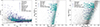 |
Fig. 1. Distribution of the TNG50-1 UDGs selected in our sample in the (left) Mg − Re, (middle) M* − Mdyn, and (right) M* − Mgas space marked in teal stars. To compare with the observed populations, the UDGs obtained from Leisman et al. (2017), Román & Trujillo (2017), Shi et al. (2017), Janowiecki et al. (2019), Marleau et al. (2021), Kadowaki et al. (2021), Poulain et al. (2022), and Jones et al. (2023) are superposed on the left panel. Similarly, on the middle and the right panel, the stellar, dynamical, and gas masses of the UDGs taken from Guo et al. (2020), Mancera Piña et al. (2020), Karunakaran et al. (2020), Marleau et al. (2021), Kong et al. (2022), and Kado-Fong et al. (2022) are shown for comparison. The teal dots represent the remaining UDGs identified in TNG50-1 while the grey dots denote the whole sample space from which the UDGs were selected. |
Our LSB sample consists of the non-dwarf subset of the low-surface brightness galaxies which are characterised by their higher asymptotic velocities (Vmax; de Blok et al. 1996; McGaugh et al. 1995). The UDGs and the LSBs are often considered and studied on an equal footing in the literature (see for example Martin et al. 2019; Kado-Fong et al. 2021; Pérez-Montaño et al. 2024) since the UDG formation scenario proposed by Amorisco & Loeb (2016) is analogous to that of the LSBs (de Blok et al. 1996; McGaugh et al. 1995; Jadhav Y & Banerjee 2019). In general, the LSBs are defined to be a class of galaxies with characteristically low stellar surface densities regardless of their masses, sizes and morphologies. While an overlap may exist between the two groups, the classical late-type LSBs are distinct from the classical dwarf galaxies (van den Hoek et al. 2000; Matthews et al. 2001; O’Neil et al. 2004; Kim & Lee 2013). This is the main reason to incorporate the LSBs in our classification study. To choose the LSBs in our sample, we limited the Vmax within the range 100−200 km s−1 and MB > −18.5 (Impey et al. 1996; de Blok et al. 1996; Matthews et al. 2001; Kniazev et al. 2004). In addition, we restricted the galaxies to have M* < 109.6 M⊙ following their observed stellar mass range. In this way, we selected the 251 galaxies in our final LSB sample.
We refer to the Milky Way-like L*-type galaxies as the HSBs in our study and identified them based on their M* and Vmax. We selected 300 galaxies in our final HSB sample, which satisfied the following selection criteria: M* > 109.7 M⊙ and 170 < Vmax < 250 km s−1 (Cooray & Milosavljević 2005; Pizzella et al. 2005; Robotham et al. 2013).
Finally, we chose our dwarf sample from the set of low-luminosity galaxies with Mg > −17 and M* ∼ 106 − 9 M⊙ (Revaz & Jablonka 2018; Poulain et al. 2022). To avoid overlap with the UDGs, our dwarf samples were chosen to have Re < 1.5 kpc. Similar to the case of the UDGs, we imposed a resolution criterion of 3000 stellar particles, therefore ending up with 538 dwarf galaxies in our final sample. Here, in all cases, M*, Mgas, and MDM represent the total stellar, gas, and DM masses of a galaxy. Therefore, to list the mass properties of our galaxy samples from the TNG data archive, we chose those definitions which consider all the (star or DM) particles/(gas) cells bound to a galaxy sub-halo. A similar argument holds for Mg and MB as well.
3. Methods
3.1. Analysis of the local environment
In TNG50, the usual convention to distinguish the field galaxies from the satellites relies on the FOF and SUBFIND algorithm. Although it provides a qualitative classification of galaxies as either ‘central’ or ‘satellite’3, it may not be sufficient to quantify the tidal influence of the local environment on a galaxy. For a robust classification of the environment, we employed an observationally motivated approach, i.e. by evaluating the dimensionless tidal index, Θ, for each galaxy (Karachentsev et al. 2004, 2013, 2018; Besla et al. 2018; Mutlu-Pakdil et al. 2024; Bhattacharyya et al. 2025). Θi determines the influence of the local tidal field on the i-th galaxy by finding out the maximum gravitational force (Fi, n) exerted on it by one of its 5 massive, nearest neighbours with a dynamical mass Mdyn, n located at a distance di, n (Fi, n ∼ Mn/di, n3). Θi can be expressed as follows:
 (2)
(2)
The galaxy with the strongest gravitational influence is termed as the main disturber (MD). The constant C = −10.96 is chosen such that the Keplerian period of a galaxy about its MD becomes equal to the Hubble time and the galaxy remains within a ‘zero velocity sphere’. Θi = 0 can also be regarded as the density enhancement about the i-th galaxy (Δρi, n ∼ Mn/di, n3) caused by its MD which reduces to the critical density of the universe for Θi = 0 (Karachentsev & Makarov 1999; Karachentsev et al. 2013). The galaxies with Θi < 0 can be termed as isolated and undisturbed by the environment and Θi > 0 can be considered as tidally bound to the MD; larger the Θ, stronger the local tidal influence.
To calculate Θ, we listed the 3D positions and the total dynamical masses of 18 850 galaxies with M* > 107 M⊙ and imposed the scipy.spatial.cKDTree algorithm to find the nearest neighbours with M* > 109.5 M⊙. To account for the periodic boundary conditions, the masses and positions of the galaxies within the TNG50 box were mirrored along all directions such that the original box at the centre was surrounded by 26 replicas (eight in the same plane as the original box, nine above, and nine below). Both the original and mirrored galaxies were considered when identifying the nearest massive neighbours to evaluate Θ using Eq. (2). Since the goal was to determine the nearest neighbours, the Θi values of most galaxies remain unaffected by this mirroring process, except for the relevant ones located near the boundaries. Furthermore, we labelled galaxies with Θ < 0.25 as isolated and those with Θ > 1.5 as tidally bound, while rejecting galaxies with Θ in the range 0.25−1.5. The rationale behind this selection criteria is two-fold: (1) to differentiate the isolated galaxies from the tidally bound ones, and (2) to eliminate galaxies possibly in the process of transitioning from isolated to tidally influenced scenarios. It is important to highlight that Θ = 0 is not a rigid boundary; galaxies with positive yet close-to-zero Θ values may not differ significantly from those with negative Θ values tending towards zero. A comparable argument holds for tidally bound galaxies as well: galaxies with smaller Θ, which can be referred to as transition populations, may be significantly different from highly tidally influenced galaxies (with higher Θ values). Hence, the aforementioned selection criteria in Θ allow the division of each sample into two fairly distinct sub-samples of isolated and tidally bound galaxies, thereby eliminating the transition populations. With this, the numbers of galaxies in our UDG, LSB, HSB, and dwarf samples are finalised as 235 (58 isolated, 177 tidally bound), 159 (103 isolated, 56 tidally bound), 213 (69 isolated, 144 tidally bound), and 368 (195 isolated, 173 tidally bound), respectively. The distributions of the tidal indices for our galaxy samples, along with their box plots (obtained using the python module PtitPrince) are presented in Fig. 2 (Allen et al. 2018). The light blue region represents the galaxies that were excluded from our samples. The overall distribution of our galaxy samples within the TNG50-1 box are presented in Fig. B.1. Here, it is worth noting that the UDGs are more prevalent in the tidally bound region compared to the other galaxy samples, suggesting that the tidal field may be an important factor in their origin. Finally, for a basic comparison among the chosen galaxies in our sample, we present the histograms of M*, Mgas, Mdyn and Mg in Fig. 3. The colour scheme of the histograms are as follows: UDGs in teal, LSBs in yellow, HSBs in blue, and dwarfs in pink. Furthermore, the solid and the dotted lines represent the isolated and the tidally bound sub-samples, respectively. The filled lower triangles at the top of each panel indicate the medians of the distributions for the isolated galaxy sub-samples, while the empty ones represent the medians for the tidally bound sub-samples. The same colour code and line styles are used throughout the paper.
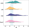 |
Fig. 2. Distribution of the tidal index, Θ, for our galaxy samples. The UDGs are in teal, LSBs are in yellow, HSBs are in blue, and the dwarfs are in pink, along with their box plots. The blue region shows the buffer region that we rejected from our study. |
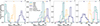 |
Fig. 3. Histograms of (a) M*, (b) Mgas, (c) Mdyn, and (d) Mg of the UDGs, LSBs, HSBs, and the dwarfs considered in our study presented in teal, yellow, blue, and pink, respectively. The solid histograms represent the isolated galaxies, and the dotted histograms denote the tidally bound sub-samples. The medians of the isolated and tidally bound sub-samples are respectively denoted with solid and hollow triangles at the top of the panels using the same colour scheme. |
3.2. Intrinsic morphology
We studied the intrinsic morphology of the DM and stellar components of our galaxy samples by solving eigenvalues and eigenvectors of the second moment of the mass distribution, the matrix known as the shape tensor in the literature (Tomassetti et al. 2016; Chua et al. 2019, 2022; Cataldi et al. 2021). The ij-component of the shape tensor is defined as  , where mn is the mass of the n-th particle,
  is the total mass, and rn, i and rn, j are the i-th and j-th component of its position vector (i, j = x, y, z). By construction, the shape tensor can be dominated by the particles located in the outer region, particularly in systems with smaller numbers of stellar and dark-matter particles (as in case of our UDG and dwarf samples). Therefore, we employed the reduced shape tensor,
 (3)
(3)
where each rn, i and rn, j is weighted by the radial distance of the particle,  . Theoretically, the eigenvalues of the shape tensor are proportional to the squares of the semi-major (a), semi-intermediate (b) and semi-minor (c) axes such that a > b > c and the corresponding eigenvectors align with the principal axes of the underlying ellipsoidal shape distribution. The shape tensor is solved iteratively in order to adopt the intrinsic shape of the matter distribution with each step.
For the shape estimation, we considered the DM (stellar) particles lying within a spherical volume of radius twice the DM (stellar) half-mass radius, Rh, DM (Rh, *), which was estimated based on the 3D particle distribution in a left-handed coordinate system centred at the galactic centre of mass. Here, we note that Rh and R1/2 (mentioned in Sect. 2) are different in the sense that R1/2 was directly noted from the TNG data archive; on the other hand, we calculated Rh based on the distribution of particles in the individual galaxy cut-outs. Following Tomassetti et al. (2016), first we computed eigenvalues and eigenvectors of the shape tensor of a spherical volume of radius R = 2Rh, fixing a = b = c = R. Then at each iteration, (a) the coordinate system was rotated such that it aligned along the eigenvectors from the previous iteration, (b) the eigenvalues were normalised with respect to the largest one (a) while fixing a = R, and (c) the particles within the ellipsoidal volume  were considered for the next iteration. The loop continued until the percentage error in b/a and c/a between two successive iterations decreased below 1% for the DM and 8% for the stellar component. In some cases, the shape tensors may fail to converge if two of the axes attain nearly equal lengths or when the convergence radius is not implemented (Allgood et al. 2006; Chua et al. 2019); also relaxing the convergence criterion may also aid in achieving convergence.
We obtained the elongation (e), flattening (f), and the triaxiality parameter (T) of the DM and stellar morphology by using the following formulae:
 (4)
(4)
All of these parameter can have values ranging between 0 and 1. Larger values of e and f represents highly elongated and flattened shapes, respectively. Further, T < 1/3, 1/3 < T < 2/3 and T > 2/3 corresponds to the oblate, triaxial and prolate shape.
3.3. Kinematical properties involving velocity dispersion
3.3.1. Velocity anisotropy parameter
To probe the orbital structure of the DM and stellar components of the galaxies in our sample, we studied their velocity anisotropy parameter (β) as a function of galactocentric radii following the definition (Binney 1980)
 (5)
(5)
Here, σr, σθ and σϕ represent the diagonal components of velocity dispersion tensor in the spherical rest-frame. We started with a coordinate transformation from Cartesian to a new left-handed orthogonal coordinate system where the z-axis aligned with the direction of angular momentum and the x − y lying arbitrarily in the plane perpendicular to z (essentially the galactic plane). Next, the Cartesian velocity components (vx, vy and vz) were converted to those in the spherical coordinates (vr, vθ and vϕ). Further, we used the following formula to calculate σr, σθ and σϕ at 15 radial points equally spaced between 0 and 2Rh by considering the particles within each spherical shell:
 (6)
(6)
From Eq. (5), it is evident that the β parameter is defined in such a manner that it can attain values between −∞ and 1. β = −∞ and β = 1 represent, purely tangential and purely radial orbits, respectively, while β = 0 describes an isotropic orbital structure.
3.3.2. Stellar velocity ellipsoid:
We further studied the components of the stellar velocity dispersion in the cylindrical rest-frame (σr, σθ, σz) whose ratios define the shape of the stellar velocity ellipsoid (Schwarzschild 1907; Gerssen et al. 1997; Shapiro et al. 2003; Gerssen & Shapiro Griffin 2012). In a similar manner as discussed in Sect. 3.3.1, we evaluated σr, σθ and σz in the cylindrical coordinates and evaluated their ratios – σz/σr, σθ/σr – as a function of galactocentric radius up to 2.5Rh. σz/σr > 0.5 and < 0.5 are suggestive of, respectively, dynamically hot and cold stellar components revealing key information about the underlying kinematic heating mechanisms. The effects of vertical disc heating agents (for example, galactic bars) increases the σz/σr, on the other hand, non-axisymmetric features such as spirals can cause decrease in σz/σr (Pinna et al. 2018 and the references therein). In general, σθ/σr only validates the epicyclic approximation projected to the plane of the galactic disc. However, σθ/σr may be crucial to understanding the variations in stellar orbital trajectories, therefore, inferring the differences in the underlying halo potential (Combes et al. 2002; Binney & Tremaine 2008). It may also indicate the presence of bulge or bar-like structures in a galaxy (Pinna et al. 2018; Chemin 2018; Walo-Martín et al. 2022).
3.4. Kinematical properties extracted from mock IFS data cubes
In our study, we employed the publicly available R-software framework SimSpin to simulate mock IFS data using the TNG50-1 galaxy cut-outs as initial conditions (Harborne et al. 2020, 2023). The LOSVD f(v) of a galaxy reveals the distribution of stellar motions projected along the line-of-sight and can be extracted from its IFS data cube. The LOSVD of a galaxy can be parametrised with a Gaussian and higher-order (> 2) GH functions (Gerhard 1993; van der Marel & Franx 1993) as
 (7)
(7)
Here, I0 is a normalisation constant; vfit and σfit are the measured radial velocity and velocity dispersion, respectively, while v is the mean radial velocity with  . ℋ3 and ℋ4 represent the third and fourth order Hermite polynomials. The coefficients associated with ℋ3 (h3) and ℋ4 (h4) in Eq. (7) quantify the deviation of the LOSVD from a standard Gaussian velocity distribution. In general, the IFS data cubes are binned by implementing the Voronoi 2D-binning algorithm vorbin (Cappellari & Copin 2003) and fitted using ppxf scheme (Cappellari & Emsellem 2004) to extract the pixel-by-pixel velocity moment maps. However, SimSpin offers a choice to generate the line-of-sight velocity (V), dispersion (σ), h3, and h4 moments directly (only up to the fourth order).
SimSpin generates the mock IFS spectra by implementing three main functions – (1) telescope that can be set to mimic the instrumental specifications of some well-known IFS survey like MUSE, CALIFA, MANGA, SAMI; (2) observing_strategy that defines the distance, inclination etc. of a galaxy; and (3) build_datacube that generates the spectral data cubes or kinematic moment maps specified by method for a given telescope specifications and observational conditions. In this work, we set the telescope type to match the MUSE survey while applying g-band SDSS filter bandpass function (filter = ‘g’) and adding some artificial ‘noise’ such that signal_to_noise ratio ∼30. The field-of-view (fov) was chosen suitably for different galaxy populations based on their radial extent. Next, the galaxies were specified to be observed at a projected redshift-distance (dist_z) of 0.05, inclined at angles (inc) 10° and 50°. Finally, the mass-weighted 2D maps of the velocity moments were constructed by setting method = velocity, mass_flag = T and turning on the particle-based Voronoi tessellation (voronoi_bin = T). To minimise the effect of shot-noise on the mock IFS data cubes, we restricted each Voronoi pixel to contain a minimum (voronoi_limit) of 200 particles (Harborne et al. 2024).
To avoid using effective radii obtained from the 3D stellar-particle distributions (as discussed in Sect. 2), we used the 2D-flux distribution of the datacubes inclined at angle 10° to obtain the effective radii. Additionally, the galaxy datacubes with 50°-inclination were employed to find the projected ellipticity. However, to extract the stellar kinematic properties, we used only the velocity moment map which were constructed for the 50° inclination. We fitted Sérsic model to the 2D-observed flux distribution of a galaxy at its face-on orientation while choosing the pixel with the highest mass as the centre of the 2D map. The R1/n model proposed by Sérsic (Sérsic 1963; Sersic 1968) expresses the intensity of light as a function of galactocentric radius as
![Mathematical equation: $$ \begin{aligned} I(R) = I_e \; \mathrm{exp} \bigg \{-b_n \bigg [\bigg (\frac{R}{R_{\mathrm{eff} }}\bigg )^{\frac{1}{n}} - 1\bigg ]\bigg \}, \end{aligned} $$](/articles/aa/full_html/2026/03/aa56109-25/aa56109-25-eq13.gif) (8)
(8)
where, Ie represents the intensity at the effective radius, Reff, n is the Sérsic index, and the constant bn = 2n − 1/3. Next, we constructed the inertia tensor of the 2D-flux distribution to estimate the alignment (ϑ) of the principal axes with respect to the 2D Cartesian x − y (following Carter & Metcalfe 1980). The formula for obtaining ϑ is given by
 (9)
(9)
Here, (xi, yi) and Fi represent the coordinate and the flux of the i-th pixel on the 2D map considering all the valid pixels. Further, we calculated the projected ellipticity of the galaxy inclined at an angle of 50° using the following expression (Emsellem et al. 2007):
 (10)
(10)
keeping x and y aligned along the photometric major and minor-axis, respectively. Here, N represents the total number of pixels within 2.5 Reff. We further extracted the kinematic properties such as ⟨V/σ⟩, proxy of the spin parameter (λRe), ⟨h3⟩, and ⟨h4⟩. For each of the aforementioned parameters, the ⟨ ⟩ symbol represents the flux-weighted mean evaluated within an elliptical region of semi-major axes, Reff, and ellipticity, ϵ, inclined at an angle, ϑ, with respect to x − y, as follows (Emsellem et al. 2007):
 (11)
(11)
Here, we note that the dwarfs in our sample are comparatively less extended than the other galaxy populations. Therefore, we considered 2 Reff for obtaining the flux-weighted averages for the dwarf sample. Further, the following formulae were implemented to calculate V/σ and λRe (Binney 2005; Emsellem et al. 2007; Cappellari et al. 2007):
 (12)
(12)
 (13)
(13)
Here, Ri is the distance to the i-th pixel in the elliptical region. In the Eqs. (12) and (13), we used the inclination-corrected velocity by substituting V with V/cos 50 to incorporate the circular velocity in these expressions. Equation (12) characterises the ratio of ordered to random motion: V/σ > 1 signifies the dominance of rotational motions observed in fast-rotating (FRs) galaxies and V/σ < 1 suggests the influence of dispersion suggestive of slow-rotating (SRs) galaxies. Moreover, λRe is a measure for the galaxy’s global rotation that can be employed to investigate the kinematic features of the galaxy. Similarly, λRe > and < 0.1 roughly indicates the FRs and the SRs, respectively. Finally, the average of the coefficient h3 measures the global asymmetry in the velocity distribution such that ⟨h3⟩ > 0 (< 0) describes skewness towards velocities lower (higher) than the mean velocity of the galaxy. Parallelly, the average of ⟨h4⟩> 0 corresponds to an overall heavy-tailed distribution with sharper peak, whereas ⟨h4⟩< 0 indicates an overall light-tailed blunt distribution compared to the standard Gaussian (Halliday et al. 2001; van de Sande et al. 2017).
4. Results and discussion
We present our results in three main segments divided based on the analysis techniques. In Sect. 4.1, we study possible scaling relations between a few pairs of mass properties which were directly noted from the TNG archive. In Sects. 4.2 and 4.3, we discuss the morphological, orbital and kinematical properties of our galaxy samples obtained by analysing the galaxy cut-outs. Finally, we explore the kinematic properties extracted from the mock IFS data cubes in Sect. 4.4. In all the cases, we primarily focus on the intrinsic properties of the UDGs and observe their similarities and differences with other galaxy populations.
4.1. Possible galaxy scaling relations
Galaxies may appear similar by means of individual parameters; however, the differences in their origin are reflected in the galaxy scaling relations, which are regulated by the underlying physical processes (da Costa & Renzini 1996). In Fig. 4 we present a set of possible scaling relations obtained separately for the isolated and tidally bound subsets of our galaxy samples. On each panel, scatter distributions and regression fits for the isolated galaxies are plotted with solid circles and solid lines, respectively; those of the tidally bound galaxies are denoted with empty circles and dotted lines. We followed the same colour scheme for our galaxy populations as discussed in Sect. 3.1. For each pair of parameters, we obtained the ordinary regression relation using the python module statsmodels and noted the coefficient of determination (R2) and the corresponding p-value. The null hypothesis in this case states that there exists no correlation between the independent and the dependent variables. p < 0.05 rejects the null hypothesis thereby suggesting a possible correlation, while, p > 0.05 offers no conclusion. In parallel, we examined validity and strength of the correlation between each pair of parameters by conducting Spearman’s rank correlation test by employing the python module scipy. Again, we wrote down Spearman’s correlation coefficient (hereafter denoted by S) and the corresponding p values. Similar to the previous case, p < 0.05 rejects the null hypothesis revealing a monotonic correlation between two physical parameters. For a statistically significant correlation, positive and negative signs of the S-coefficient denote, respectively, correlations and anti-correlations; the larger the absolute value of S, the stronger the (anti-)correlation. We assumed a threshold of 0.5 for S above which a correlation was termed to be stronger. The slopes (m), intercepts (c), R2 and the S-coefficients are listed in Table C.1. The p-values are smaller than 0.05 in all cases, unless mentioned. We observed that in cases of mild (anti-)correlations where S < 0.5, the R2 values are significantly smaller. Therefore, we considered the S-coefficients as the indicators of correlations and use the m and c-values to differentiate between the galaxy populations.
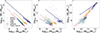 |
Fig. 4. Possible scaling relations of (a) stellar-to-gas mass ratio versus gas mass (log10M*/Mgas vs. log10Mgas), (b) stellar-to-gas mass ratio versus total dynamical mass (log10M*/Mgas vs. log10Mdyn), and (c) total baryonic mass versus total dynamical mass (log10Mb vs. log10Mdyn). The UDGs, LSBs, HSBs, and the dwarfs are shown in teal, yellow, blue, and magenta colours, respectively. Each of the galaxy samples are divided into two sub-samples – isolated (denoted with filled circles) and tidally bound (denoted with empty circles). The scaling relations are obtained for the two sub-samples of each galaxy classes separately and plotted with solid and dashed lines, respectively. |
Panel a of Fig. 4 presents the correlation between stellar-to-gas mass ratio, M*/Mgas and Mgas for our galaxy samples. The gas mass present in a galaxy constitutes the fuel for star formation and the stellar mass characterises the final outcome of the past star formation activities. The correlation between M*/Mgas and Mgas can be studied to understand how efficiently the gas is converted to stars for a given Mgas, and therefore, M*/Mgas may be considered as a proxy of star formation efficiency. We observed strong anti-correlations between these two parameters (S-values ≲ −0.6) for all the galaxy populations. Here, we note that the regression fits for the UDGs and the dwarfs are almost identical. It is also evident that the UDGs and the dwarfs have significantly lower M*/Mgas values for a given Mgas compared to the HSBs; this is similar to what has been suggested for the low-mass dwarf galaxies (Catinella et al. 2018; Dou et al. 2024, 2025). On the other hand, LSBs seem to constitute an intermediate population. Hence, we may infer that the star formation activities in the UDGs and the dwarfs are reasonably different than that of the LSBs and the HSBs.
Dark matter may have an important role in regulating the star formation activities in galaxies, especially in case the DM-dominated galaxy populations (Garg & Banerjee 2017). Therefore, we studied how M*/Mgas varies as a function of Mdyn in panel b of Fig. 4. M*/Mgas anti-correlates with Mdyn as suggested by their S-values. Here we observe that the p-values associated with R2 and S for the isolated UDGs and the isolated HSBs are greater than 0.05, making the correlation statistically insignificant. Hence, based on their distributions in this parameter space, we note that the UDGs and dwarfs cluster in a similar region in contrast to the other galaxy populations. This suggests that the influence of DM on the star formation activities in the UDGs and the dwarfs are almost alike.
Finally, in panel c of Fig. 4, we observe the correlation between the baryonic mass, Mb and Mdyn, analogous to the baryonic Tully-Fisher relation (McGaugh et al. 2000; McGaugh 2005). Here, we obtained the total baryonic mass as Mb = M* + Mgas. As expected, all the galaxy populations show a strong correlation between these two parameters with correlation coefficients > 0.6. The distribution of the UDGs and the dwarfs and their regression fits are nearly similar in this parameter space. Interestingly, the baryon content in the UDGs seems to be ‘normal’, in contrary to the baryon-rich field UDGs studied by Mancera Piña et al. (2019).
Therefore, we observe that the UDGs and the dwarfs follow nearly similar scaling relations which are significantly different from that of the HSBs. This corroborates the idea that the UDGs and the dwarfs share a common dynamical origin, in contrast to the failed L*-type galaxy formation scenario. Here, it is worth-noting that a clear bimodality is observable in the way the LSB galaxies are distributed in these spaces. Some of the LSBs lie closer to the regression fits for the UDGs and the dwarfs. These may represent the transition population between late-type classical LSBs and LSB-dwarfs. Thus, there is a possibility that UDGs are transformed from these type of LSBs.
4.2. Intrinsic morphology of the DM and stellar components
The intrinsic shape of the DM distribution reveals important insights to the halo and baryon assembly history, effects of the baryonic feedback mechanisms and the surrounding environment (see for example, Cataldi et al. 2021; Orkney et al. 2023; Rodriguez et al. 2024 and the references therein). The shape of the DM halo modifies the underlying halo potential and thus deeply impacts the stellar orbits as well as the stellar morphology of a galaxy (Zotos 2014; Zotos & Caranicolas 2014). Therefore, it is an important parameter to constraint the picture of galaxy formation and evolution. In Fig. 5 we present the intrinsic shapes of the DM halos of the UDGs, LSBs, HSBs, and the dwarfs from left to right panels, respectively. The distribution of the intermediate-to-major (b/a)DM and minor-to-major (c/a)DM axes ratios of the DM distribution is shown on the top row. The colour code has been maintained as described in Sect. 3.1. The histograms of x and y-data on each panel are shown on the top and right of the panel. For a better comparison, the histograms are plotted with same bin widths for all the galaxy classes and represent the fraction of occurrences in each bin. More than 70% of the UDGs, LSBs, HSBs, and the dwarfs (in both isolated and tidally bound conditions) have (b/a)DM values within the range 0.9−1 and (c/a)DM ranging between 0.75 and 0.95. For a clearer classification, the elongation (eDM) and flattening (fDM) of the DM distribution is shown in the bottom row of Fig. 5. The eDM − fDM spaces are divided into four quadrants with the following approximate ranges: (i) spherical (S) for 0 ≲ eDM ≲ 0.5 & 0 ≲ fDM ≲ 0.5; (ii) oblate (O) for 0 ≲ eDM ≲ 0.5 & 0.5 ≲ fDM ≲ 1; (iii) prolate (P) for 0.5 ≲ eDM ≲ 1 & 0 ≲ fDM ≲ 0.5 and (iv) triaxial (T) for 0.5 ≲ eDM ≲ 1 & 0.5 ≲ fDM ≲ 1 (Tomassetti et al. 2016). Most of the galaxies in UDG, LSB, HSB and dwarf samples are observed to reside in spherical DM halos as suggested by their eDM and fDM values. In both cases, no striking differences can be identified based on their distributions in the (b/a)DM–(c/a)DM and eDM − fDM spaces.
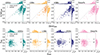 |
Fig. 5. Distribution of the (top) intermediate-to-major axes ratios versus minor-to-major axes ratios ((b/a)DM–(c/a)DM) and (bottom) elongation and flattening (eDM − fDM) of the DM component of our galaxy samples. The histograms of the x and y data are plotted on the top and right sides of each panel, respectively, with equal bin widths, showing the fraction of galaxies in each bin. The isolated galaxies are shown with filled circles and filled histograms, while the empty circles and empty histograms represent the tidally bound sub-samples. The same colour scheme as in Fig. 4 is adopted. |
Stellar morphology of a galaxy preserves imprints of its formation mechanisms and reveals important information about the intrinsic and extrinsic physical mechanisms influencing its evolution (Rodriguez-Gomez et al. 2017; Emami et al. 2021; Zhang et al. 2022; Kolesnikov et al. 2025 and the references therein). Based on the existing morphological classifications, galaxies can be broadly classified in two categories: elliptical or dispersion-supported early-type galaxies (ETGs) and disc or rotation-supported late-type galaxies (LTGs) – both being the relics of distinct formation mechanics (Hubble 1926, 1936; Liller 1966; Kormendy & Bender 1996). In Fig. 6, the stellar shape parameters for the UDG, LSB, HSB, and dwarf samples are shown, following the same colour scheme as earlier. As discussed in Sect. 3.2, the stellar shape tensor did not converge for 23 out of 235 UDGs (14 isolated, 9 tidally bound), 52 out of 159 LSBs (36 isolated, 16 tidally bound), 52 out of 213 HSBs (25 isolated, 27 tidally bound), and 160 out of 368 dwarfs (108 isolated, 52 tidally bound). Therefore, the results are presented only for the galaxies for which the stellar shape tensor converged. The axes ratios of the stellar shapes ((b/a)* and (c/a)*) are shown in the top row of Fig. 6. On each panel, the (b/a)*–(c/a)* space is divided into three sections relating to three different morphological types: (i) spherical (S) for a* ∼ b* ∼ c*; (ii) discy/oblate (D) for a* ∼ b* > c* and (iii) elongated/prolate (E) for a* > b* ∼ c* (van der Wel et al. 2014; Zhang et al. 2022). The bottom row of Fig. 6 shows the elongation and flattening of the stellar shape distributions (e* − f*). From the distributions of our galaxy samples in these two parameter spaces, we note that isolated UDGs predominantly exhibit prolate-to-triaxial shapes, whereas they display a wider range of morphologies under tidally bound conditions. In contrast, the stellar components of dwarfs are better described by prolate shapes. The LSBs and HSBs, on the other hand, are more likely to display triaxial shapes isolated and tidally bound environments.
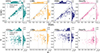 |
Fig. 6. Distribution of the stellar component of our galaxy samples in (top) (b/a)*–(c/a)* and (bottom) e* − f* spaces. The plotting scheme is similar to Fig. 5. |
For a comprehensive understanding of the overall picture, we show the distributions of the stellar (T*) and dark matter triaxiality parameters (TDM) in Fig. 7. To examine the similarities in the intrinsic dark matter and stellar shapes between the UDGs and the other galaxy samples, we performed two-sample Anderson–Darling (AD) tests using T* and TDM. For each parameter: (1) we randomly sampled 500 values with replacement from each galaxy class; (2) conducted AD tests between pairs of classes, subdivided into isolated and tidally bound sub-samples – (UDGs and LSBs), (UDGs and HSBs), and (UDGs and dwarfs) – and recorded the AD coefficients and corresponding p-values; and (3) repeated this process 5000 times and computed the median AD coefficients and p-values. The null hypothesis in this statistical test states that the shape parameters for the UDGs and the comparison galaxy samples (LSBs, HSBs, or dwarfs) follow the same continuous distribution. The null hypothesis was rejected if the AD coefficient ≥ critical value (ADcrit = 2.718 at a 2.5% significance level) with a p-value < 0.02, thereby indicating that the distributions of the corresponding parameters for the UDGs and the other galaxy samples are statistically distinct. We find that the median AD coefficients exceed ADcrit, and the p-values are below 0.02 for both T* and TDM across all pairs, except for the isolated UDGs and dwarfs. For these former cases, the null hypotheses are rejected, indicating that the distributions of the respective parameters are statistically distinct; in contrast, the null hypothesis cannot be rejected for the latter case. It may suggest that the UDGs and the dwarfs originate in DM halos of similar intrinsic shapes.
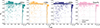 |
Fig. 7. Distribution of the stellar component of our galaxy samples in T* − TDM space. The plotting scheme is similar to Fig. 5. |
Our results for the isolated UDGs seem to be in compliance with the inferences drawn by Jiang et al. (2019) who studied the field UDGs in the NIHAO simulation and concluded that multiple stellar feedback episodes may be responsible for their non-rotating prolate shapes. On the contrary, follow-up studies incorporating the isolated UDGs in the NIHAO simulation conducted by Cardona-Barrero et al. (2020) suggest that the existence of dispersion-supported triaxial/prolate UDGs and rotation-supported oblate-discy UDGs are almost equally probable. Liao et al. (2019) also found that star-forming (blue) field UDGs in the Auriga simulation tend to have discy-shape similar to the classical low-surface brightness galaxies (LSBs), while the quenched (red) satellite UDGs acquire a prolate-shape possibly due to tidal effects. On a similar note, Van Nest et al. (2022) studied field UDGs from the ROMULUS25 and ROMULUS C simulation and observed that the isolated UDGs exhibit oblate-triaxial shapes in contrast to their non-UDG counterparts. Our results obtained for the isolated UDGs seem to be in contrast with these studies. On the other hand, the shapes of the tidally bound UDGs in our study are in compliance with the cluster UDGs studied in the literature. By studying the projected axial ratios of the Coma UDGs, Burkert (2017) observed that the UDGs exhibit more elongated, bar-like prolate shapes. Rong et al. (2020) observed that the low- and intermediate-redshift cluster UDGs display an oblate-triaxial shape and become puffier with (i) decreasing redshift, possibly indicating a ‘discy’ origin and (ii) decreasing cluster-centric distance, suggesting a crucial role of tidal interactions on their evolution. A somewhat similar observation was made by Kado-Fong et al. (2021) that the UDGs are well-characterised by the oblate-spheroid shape, irrespective of their colour or environment. Studying the cluster UDGs from the ROMULUS25 and ROMULUS C simulation, Van Nest et al. (2022) suggested that the tidal field make these galaxies relatively spherical. Therefore, we may infer that the UDGs have intrinsically prolate stellar distributions in isolation, possibly due to episodic stellar feedback. However, in a denser environment, the tidal field transforms their stellar distributions, therefore giving rise to a range of intrinsic shapes. In this context, it is important to note that our results are different compared to the inferences made by Benavides et al. (2023) on the morphologies of the UDGs in the TNG50; they found no significant difference in the shapes of the UDGs in different environments.
4.3. Orbital and kinematical properties from the galaxy cut-outs
Elements of the velocity dispersion tensor trace the dynamical status of a galaxy and are therefore crucial to probing its formation and evolution. In this section we study a few parameters constructed using the components of DM and stellar velocity dispersions that were evaluated from the individual galaxy cut-outs.
4.3.1. DM and stellar velocity anisotropy: An indicator of the underlying orbital structure
The velocity anisotropy parameter measures orbital structure of a galaxy’s DM and stellar components. The variation in β can be insightful to understand the concentration and radial distribution of DM halos (He et al. 2024 and the references therein); at the same time, the stellar velocity anisotropy may be employed to distinguish the ETGs from the LTGs (Agnello et al. 2014; Emami et al. 2022). In Fig. 8 we present the (top) DM anisotropy (βDM) as a function of galactocentric radii normalised by the DM half-mass radius. We mainly focus on the inner and middle region (up to nearly 1.5 Rh) of the DM halos as the number of particles near the outer region become significantly smaller. The solid (dashed) lines represent medians of the isolated (tidally bound) galaxy populations and the region shaded (with crossed diagonal lines) denote the 25th to 75th quartile range. By studying βDM as a function of R/Rh, we observe that the DM orbits are closer to isotropic (βDM ∼ 0) near the centre of the halo and become radial-biased (βDM > 0) with increasing radius for all the galaxy populations. In case of the UDGs, LSBs, and the dwarfs, the orbits become isotropic again while approaching the outer region. In contrast, the DM orbits continue to remain radially biased in case of the HSBs. Presence of more radial orbits near the outer halo of the HSBs may be indicative of the active radial infall of stars through accretion. On the other hand, the DM orbits of the tidally bound UDGs and dwarfs become rather tangentially biased (βDM < 0) near the outer halo maybe in response to the tidal-interactions (Vera-Ciro et al. 2014). He et al. (2024) observed that the variation in βDM depends on the total dynamical mass of the galaxies. Thus, we can conclude that the UDGs were possibly formed in lower-mass DM halos, consistent with their total dynamical mass. Similar observation can be made from the radial variation of stellar velocity anisotropies (β*) shown in the bottom row of Fig. 8. The β* profiles for the UDGs and the dwarf galaxies slowly increase with increasing radii, the LSBs displaying a slightly steeper rise. In contrast, the HSBs do not show such a gradual change: the increase in β* in their case seem to be quite steeper. The variation in β* depends on the concentration parameter (c) of the DM halo – galaxies with higher c exhibit more radially biased orbits for a given dynamical mass, therefore resulting in steeply rising radial profiles of β* – a possible signature of different assembly history or evolution (He et al. 2024). Therefore, we can speculate that the variations in the β* profiles of our galaxy samples could also be attributed to their DM c-values. However, a detailed analysis of the dark matter density distribution is necessary to confirm this hypothesis.
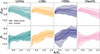 |
Fig. 8. Variation of (top) DM (βDM) and (bottom) stellar (β*) velocity anisotropy as a function of galactocentric radius normalised by the respective half-mass radius. Solid and dashed lines represent the median values of the isolated and tidally bound galaxy sub-samples, respectively. The 25th and 75th quartile regions are shown with shaded regions: solid-filled regions are for the isolated sub-samples and crossed diagonal lines are for the tidally bound ones. |
4.3.2. The components of the stellar velocity ellipsoid: Insights to the stellar kinematics
Stars in a galaxy are considered to be formed from a gas disc that settled down at the centre of a DM halo. The gas component has less velocity dispersion due to its collisional nature. However, the stars end up with gaining sufficient amount of velocity dispersion in response to the dynamical heating mechanisms. Such disc heating agents play an important role in the secular evolution of the galaxies and can be identified by the shape of the stellar velocity ellipsoid (Gerssen et al. 1997; Shapiro et al. 2003; Gerssen & Shapiro Griffin 2012). In the top and bottom panels of Fig. 9, we present the ratios of vertical-to-radial (σz/σr) and tangential-to-radial (σθ/σr) velocity dispersions as a function of galactocentric radius normalised by the stellar half-mass radius. The UDGs and the dwarfs have significantly higher values of σz/σr compared to the LSBs and the HSBs. The σz/σr values suggest that the UDGs and the dwarfs are dispersion-dominated ETGs while the LSBs and the HSBs are LTGs supported by their rotational motions (de Blok et al. 1996; Gerssen & Shapiro Griffin 2012; Adams et al. 2014). A similar observation was made in our earlier study where the HI-rich, isolated UDGs and the dwarf irregular galaxies were observed to be earlier-types compared to the LSBs (Nandi et al. 2025). We also note that range of σz/σr-values of the UDGs are quite similar to those of the Coma UDGs (Chilingarian et al. 2019). Further, the bottom row of Fig. 9 shows that the variation in σθ/σr as a function of radius. For the UDGs and the dwarfs, σθ/σr-values remain close to 1 throughout their galactic plane, indicating isotropically circular orbits. In comparison, the LSBs and the HSBs exhibit isotropic orbits near the galactic centres and the orbits become more radially biased while approaching the outer disc. The presence of increasingly radial orbits may indicate the presence of the underlying bulge or bar-like structures in the LSBs and the HSBs, which are rarer in case of the UDGs and the dwarfs (Chemin 2018; Mogotsi & Romeo 2019; Walo-Martín et al. 2022). Therefore, we conclude that the UDGs and the dwarfs exhibit similar kinematic properties, as suggested by their stellar velocity ellipsoids.
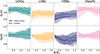 |
Fig. 9. Variation of stellar (top) vertical-to-radial (σz/σr) and (bottom) tangential-to-radial (σθ/σr) velocity dispersion ratios as a function of galactocentric radius normalised by the stellar half-mass radius. The plotting scheme is similar to Fig. 8. |
4.4. Stellar kinematics from the mock IFS spectra
The velocity (V), velocity dispersion (σ), and the higher order (h3 & h4) moment maps constitute a set of parameter space which directly explores the stellar kinematics of a galaxy (Gerhard 1993; Halliday et al. 2001; Bacon et al. 2001; de Zeeuw et al. 2002; Emsellem et al. 2004; Cappellari et al. 2007; Emsellem et al. 2007, 2011; Veale et al. 2017; Falcón-Barroso et al. 2017, 2019; van de Sande et al. 2017, 2021; Bernardi et al. 2019; Pinna et al. 2021). In this section we analysed the properties of the stellar kinematic moment maps obtained from the mock IFS spectra.
4.4.1. Stellar kinematics from first and second moments
Based on the degree of ordered motion, galaxies can be broadly classified into two categories: rotation-supported FRs and pressure-supported SRs. Emergence of these two distinct classes may be explained by the differences in their assembly histories (Cappellari et al. 2006; van de Sande et al. 2018). The top panel of Fig. 10 shows the distribution of our galaxy samples in rotation velocity-to-velocity dispersion (V/σ) versus projected ellipticity (ϵ) space. In all cases, the solid magenta and the dotted lines predict the theoretical distribution of the axisymmetric galaxies with anisotropy parameter βz = 0.7ϵ for different viewing angles – starting on the right with the solid magenta line for the edge-on galaxies to the left-most for the face-on viewing angles. The grey dashed lines, on the other hand, correspond to the theoretical distributions of galaxies with intrinsic ellipticities ϵ = 0.85 − 0.35 viewed in edge-on orientations (see Cappellari et al. 2007; Emsellem et al. 2007).
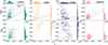 |
Fig. 10. Distribution of our galaxy samples in (top) the V/σ versus ϵ space and (bottom) the λRe versus ϵ space following the same plotting scheme as Fig. 5. The solid magenta line represents the predicted theoretical distribution of the axisymmetric galaxies with the anisotropy parameter βz = 0.7ϵ at an inclination of 90°, and dotted lines from right to left denote the theoretical distribution for decreasing inclinations. The leftmost dotted line corresponds to the face-on orientation. The grey dashed lines correspond to locations of galaxies at edge-on orientations with intrinsic ellipticities of ϵ = 0.85 − 0.35 (see Cappellari et al. 2007; Emsellem et al. 2007). |
Based on the distribution of the galaxies in the V/σ − ϵ space, we observed that the UDGs and the dwarfs are dispersion-supported systems with V/σ < 1, and therefore, they can be referred to as SRs. In comparison, the LSBs and HSBs seem to have both V/σ > 1 and < 1 with nearly equal probability suggesting that they can be both FRs and SRs. Here it is notable that the HSBs are attaining higher values of V/σ compared to the LSBs. Environment seems to have no significant impact on any of these galaxy populations as their distributions looks almost similar in case of isolated and tidally bound galaxies except for the isolated LSBs. In this context, we note that the Reff values for the UDGs obtained in Sect. 3.4 are consistent with their definition, i.e. > 1.5 kpc, with roughly 12% of the values falling below this threshold (maximum deviation being approximately 25%).
While V/σ can capture the contest between the rotation and the random motion of a galaxy in describing its stellar kinematics, it lacks the ability to identify its kinematic features and characterise the true nature of the galactic rotation. λRe, by definition, identifies the complex kinematic structures present in the stellar component and thus traces the true global rotation in the galaxy. In the bottom row of Fig. 10, we study the λRe-values of our galaxy samples with respect to their ellipticity, ϵ. The UDGs and the dwarfs are predominantly composed of slowly rotating galaxies, with nearly 50% of these populations exhibiting λRe < 0.2. In contrast, the LSBs are more strongly represented at higher values of λRe. The HSBs, on the other hand, display a broad range of λRe values, suggesting the presence of both FRs and SRs within the population. The distributions of the isolated and tidally bound galaxies in the λRe − ϵ space agrees with that of the V/σ − ϵ space, except for the isolated LSBs. The result obtained in this section is in line with what we observed in our previous study: The isolated HI-rich UDGs and the dwarf irregular galaxies are SRs compared to the LSBs, which are FRs (Nandi et al. 2025). A similar conclusion was made by Cardona-Barrero et al. (2020) by constructing projected line-of-sight velocity and velocity dispersion maps suggesting that nearly half of the field UDGs in the NIHAO simulation are FRs, the remaining half being SRs. Our results are also supported by the range of rotation properties spectroscopically observed in UDGs. Emsellem et al. (2019) conducted the first spectroscopic analysis of NGC1052-DF2 using the VLT/MUSE integral-field spectrograph and suggested it to be a prolate-rotator. van Dokkum et al. (2019) analysed the spatially resolved stellar kinematics of the Coma UDG DF44 using the Keck/DEIMOS spectrograph and observed almost no rotation. Iodice et al. (2023) reported the presence of a UDG in the Hydra I cluster, named UDG11, that shows no rotation. Additionally, Buttitta et al. (2025) investigated the stellar kinematics of 18 Hydra I UDGs and observed a range of kinematic signatures: five UDGs showed no rotation, three showed photometric major-axis rotation, and four were observed to rotate along the intermediate axis. Therefore, we infer that the UDGs and the dwarfs are distinguishable by their SR-nature as opposed to the LSBs. However, the distinction between the UDGs and the HSBs is still vague, and thus, we move one step further by investigating their higher-order velocity moments.
4.4.2. Stellar kinematics from the higher order GH moments
The correlation between h3 and V/σ varies based on the presence of rotating component in galaxies, while the presence of anisotropy in the rotation is reflected on h4. On the top row of Figure 11, we show the variation in h3 vs ⟨V/σ⟩. Here, ⟨V/σ⟩ denotes the ratio of flux-weighted average of velocity and velocity dispersion obtained by using Eq. (11). We interpret the correlation between h3 and ⟨V/σ⟩ as follows: (1) fast rotators are characterised by a strong anti-correlation between h3 and ⟨V/σ⟩; (2) non-regular or slowly rotating galaxies are distributed almost vertically in this parameter space; and (3) no clear conclusions can be drawn for galaxies that are distributed horizontally or show no particular pattern, possibly due to the coexistence of both correlation and anti-correlation arising from individual kinematic components (van de Sande et al. 2017; Naab et al. 2014). On visual inspection, a clear anti-correlation can be seen between h3 and V/σ for the LSBs and HSBs; in comparison, the distributions of the UDG and dwarf galaxies are more vertical in nature. Therefore, we may infer that the UDGs and dwarfs can be classified as slow or non-regular rotators, while the LSBs and HSBs are regular rotators, suggestive of the presence of prominent disc components. Finally, the distribution of h4 as a function of ⟨V/σ⟩ is shown in the bottom row of Fig. 11. A rounder, heart-shaped distribution in the h4 − ⟨V/σ⟩ space is observed for the regular rotators; in contrast, no such correlation is evident for the quasi- or non-regular rotators. Among our galaxy samples, the LSBs and HSBs predominantly form rounder distributions with positive h4 values, indicative of stronger rotation. Conversely, the UDGs and dwarfs show a more vertical distribution with two distinct clusters: (i) galaxies with positive h4 values spanning a range roughly half that of the LSBs and HSBs, and (ii) galaxies with negative h4 values, similar to non-rotating ellipticals (Bender et al. 1994). In this context, we note that van Dokkum et al. (2019) observed h3 = −0.03 ± 0.04 for DF44, which falls within the same range as the UDGs in our sample. However, they obtained h4 = 0.13 ± 0.05 for DF44, which is considerably higher than that of the UDGs in our sample, comparable to the HSBs. Overall, we can infer that the UDGs and the dwarfs are characterised by non-regular or slowly rotating stellar components, in contrast to the more regularly, fast-rotating LSBs and HSBs.
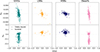 |
Fig. 11. Distribution of our galaxy samples in the (top) h3 and (bottom) h4 versus ratio of flux-weighted average of velocity and velocity dispersion (⟨V/σ⟩). A plotting scheme similar to that of the Fig. 5 has been adopted. |
5. Conclusions
In this work, we have studied the morphological and kinematical properties of the UDGs and compared them with those of the LSB, HSB, and dwarf galaxy samples. We incorporated a set of UDG, LSB, HSB, and dwarf galaxies from the TNG50-1 box for this classification study. We further divided the galaxy samples in two sub-samples of isolated galaxies and tidally bound galaxies based on their local environments. At first, we examined the correlations between the (a) stellar-to-gas mass ratio and gas mass, (b) stellar-to-gas mass ratio and total dynamical mass, and (c) total baryonic mass and total dynamical mass of our galaxy samples, and we studied their scaling relations in terms of these pairs of parameters. We observed that in most of the cases, the UDGs and the dwarfs share very similar regression relations as compared to the other galaxy populations. Next, we studied the intrinsic shape of the DM and stellar components of these galaxies by analysing their TNG50-1 galaxy cut-outs. All the galaxy classes were observed to have nearly spherical DM shapes. However, the isolated UDGs and dwarfs may follow statistically similar distributions in terms of the DM triaxiality parameter. Moreover, the isolated UDGs and the dwarf galaxies exhibit prolate shapes in comparison to the LSBs and the HSBs, which mostly have oblate-triaxial shapes. On the other hand, the UDGs in the tidally bound condition display a range of stellar morphology – from prolate to oblate. To investigate the orbital properties, we studied the DM and stellar velocity anisotropy of our galaxy samples. The variations in the DM and stellar velocity anisotropy are consistent with the differences in their dynamical mass, implying that UDGs reside in dwarf-like dark halos. Furthermore, the shapes of their stellar velocity ellipsoids suggest that the UDGs and the dwarfs are ETGs, while the LSBs and the HSBs can be characterised as LTGs. Finally, we employed the publicly available R-software SimSpin to construct the stellar kinematic moment maps of the galaxies considered in our study. Based on the flux-averaged values of the rotation-to-dispersion ratio (V/σ) and the spin parameter proxy (λRe) as functions of projected ellipticity, we can classify the UDGs and dwarfs as slow rotators, whereas the LSBs and HSBs can be identified as fast rotators. A similar inference is supported by their higher-order GH moments (h3 and h4), which indicate that the UDGs and dwarfs belong to non-regular or slowly rotating galaxy classes, in contrast to the regularly rotating LSBs and HSBs. Therefore, we can conclude that the kinematical properties of the UDGs and the dwarfs are almost alike, suggesting their common dynamical origin. We can also infer that the differences in the stellar morphologies of the UDGs and the dwarfs can be probed further to derive important constraints in explaining the evolution of the UDGs.
Acknowledgments
We acknowledge that the project is funded by the Prime Minister’s Research Fellowship with ID: 0902007. We thank the anonymous referee for his/her detailed, constructive suggestions which have improved the paper.
References
- Adams, J. J., Simon, J. D., Fabricius, M. H., et al. 2014, ApJ, 789, 63 [NASA ADS] [CrossRef] [Google Scholar]
- Agnello, A., Evans, N. W., & Romanowsky, A. J. 2014, MNRAS, 442, 3284 [NASA ADS] [CrossRef] [Google Scholar]
- Allen, M., Poggiali, D., Whitaker, K., Rhys Marshall, T., & Kievit, R. 2018, https://doi.org/10.5281/zenodo.1402959 [Google Scholar]
- Allgood, B., Flores, R. A., Primack, J. R., et al. 2006, MNRAS, 367, 1781 [NASA ADS] [CrossRef] [Google Scholar]
- Amorisco, N. C., & Loeb, A. 2016, MNRAS, 459, L51 [NASA ADS] [CrossRef] [Google Scholar]
- Bacon, R., Copin, Y., Monnet, G., et al. 2001, MNRAS, 326, 23 [Google Scholar]
- Baes, M., Mosenkov, A., Kelly, R., et al. 2024, A&A, 683, A182 [NASA ADS] [CrossRef] [EDP Sciences] [Google Scholar]
- Barbosa, C. E., Zaritsky, D., Donnerstein, R., et al. 2020, ApJS, 247, 46 [Google Scholar]
- Benavides, J. A., Sales, L. V., Abadi, M. G., et al. 2021, Nat. Astron., 5, 1255 [NASA ADS] [CrossRef] [Google Scholar]
- Benavides, J. A., Sales, L. V., Abadi, M. G., et al. 2023, MNRAS, 522, 1033 [NASA ADS] [CrossRef] [Google Scholar]
- Bender, R., Saglia, R. P., & Gerhard, O. E. 1994, MNRAS, 269, 785 [Google Scholar]
- Bernardi, M., Domínguez Sánchez, H., Brownstein, J. R., Drory, N., & Sheth, R. K. 2019, MNRAS, 489, 5633 [Google Scholar]
- Besla, G., Patton, D. R., Stierwalt, S., et al. 2018, MNRAS, 480, 3376 [NASA ADS] [CrossRef] [Google Scholar]
- Bhattacharyya, J., Peter, A. H. G., & Leauthaud, A. 2025, ArXiv e-prints [arXiv:2501.01946] [Google Scholar]
- Binney, J. 1980, MNRAS, 190, 873 [NASA ADS] [CrossRef] [Google Scholar]
- Binney, J. 2005, MNRAS, 363, 937 [Google Scholar]
- Binney, J., & Tremaine, S. 2008, Galactic Dynamics: Second Edition (Princeton: Princeton University Press) [Google Scholar]
- Burkert, A. 2017, ApJ, 838, 93 [NASA ADS] [CrossRef] [Google Scholar]
- Buttitta, C., Iodice, E., Doll, G., et al. 2025, A&A, 694, A276 [NASA ADS] [CrossRef] [EDP Sciences] [Google Scholar]
- Buzzo, M. L., Forbes, D. A., Brodie, J. P., et al. 2022, MNRAS, 517, 2231 [NASA ADS] [CrossRef] [Google Scholar]
- Buzzo, M. L., Forbes, D. A., Jarrett, T. H., et al. 2024, MNRAS, 529, 3210 [NASA ADS] [CrossRef] [Google Scholar]
- Cappellari, M., & Copin, Y. 2003, MNRAS, 342, 345 [Google Scholar]
- Cappellari, M., & Emsellem, E. 2004, PASP, 116, 138 [Google Scholar]
- Cappellari, M., Bacon, R., Bureau, M., et al. 2006, MNRAS, 366, 1126 [Google Scholar]
- Cappellari, M., Emsellem, E., Bacon, R., et al. 2007, MNRAS, 379, 418 [Google Scholar]
- Cardona-Barrero, S., Di Cintio, A., Brook, C. B. A., et al. 2020, MNRAS, 497, 4282 [NASA ADS] [CrossRef] [Google Scholar]
- Carleton, T., Errani, R., Cooper, M., et al. 2019, MNRAS, 485, 382 [NASA ADS] [CrossRef] [Google Scholar]
- Carter, D., & Metcalfe, N. 1980, MNRAS, 191, 325 [CrossRef] [Google Scholar]
- Cataldi, P., Pedrosa, S. E., Tissera, P. B., & Artale, M. C. 2021, MNRAS, 501, 5679 [NASA ADS] [CrossRef] [Google Scholar]
- Catinella, B., Saintonge, A., Janowiecki, S., et al. 2018, MNRAS, 476, 875 [NASA ADS] [CrossRef] [Google Scholar]
- Chemin, L. 2018, A&A, 618, A121 [NASA ADS] [CrossRef] [EDP Sciences] [Google Scholar]
- Chilingarian, I. V., Afanasiev, A. V., Grishin, K. A., Fabricant, D., & Moran, S. 2019, ApJ, 884, 79 [NASA ADS] [CrossRef] [Google Scholar]
- Chua, K. T. E., Pillepich, A., Vogelsberger, M., & Hernquist, L. 2019, MNRAS, 484, 476 [Google Scholar]
- Chua, K. T. E., Vogelsberger, M., Pillepich, A., & Hernquist, L. 2022, MNRAS, 515, 2681 [NASA ADS] [CrossRef] [Google Scholar]
- Combes, F., Boisse, P., Mazure, A., Blanchard, A., & Seymour, M. 2002, Galaxies and Cosmology (Springer Science& Business Media) [Google Scholar]
- Cooray, A., & Milosavljević, M. 2005, ApJ, 627, L89 [Google Scholar]
- da Costa, L. N., & Renzini, A. 1996, Galaxy Scaling Relations: Origins, Evolution and Applications (Berlin: Springer-Verlag) [Google Scholar]
- Davis, M., Efstathiou, G., Frenk, C. S., & White, S. D. M. 1985, ApJ, 292, 371 [Google Scholar]
- de Blok, W. J. G., McGaugh, S. S., & van der Hulst, J. M. 1996, MNRAS, 283, 18 [NASA ADS] [CrossRef] [Google Scholar]
- de Zeeuw, P. T., Bureau, M., Emsellem, E., et al. 2002, MNRAS, 329, 513 [Google Scholar]
- Di Cintio, A., Brook, C. B., Dutton, A. A., et al. 2017, MNRAS, 466, L1 [NASA ADS] [CrossRef] [Google Scholar]
- Dolag, K., Borgani, S., Murante, G., & Springel, V. 2009, MNRAS, 399, 497 [Google Scholar]
- Dou, J., Peng, Y., Gu, Q., et al. 2024, ApJ, 973, L23 [Google Scholar]
- Dou, J., Peng, Y., Gu, Q., et al. 2025, ApJ, 982, L12 [Google Scholar]
- Emami, R., Genel, S., Hernquist, L., et al. 2021, ApJ, 913, 36 [NASA ADS] [CrossRef] [Google Scholar]
- Emami, R., Hernquist, L., Vogelsberger, M., et al. 2022, ApJ, 937, 20 [Google Scholar]
- Emsellem, E., Cappellari, M., Peletier, R. F., et al. 2004, MNRAS, 352, 721 [Google Scholar]
- Emsellem, E., Cappellari, M., Krajnović, D., et al. 2007, MNRAS, 379, 401 [Google Scholar]
- Emsellem, E., Cappellari, M., Krajnović, D., et al. 2011, MNRAS, 414, 888 [Google Scholar]
- Emsellem, E., van der Burg, R. F. J., Fensch, J., et al. 2019, A&A, 625, A76 [NASA ADS] [CrossRef] [EDP Sciences] [Google Scholar]
- Falcón-Barroso, J., Lyubenova, M., van de Ven, G., et al. 2017, A&A, 597, A48 [NASA ADS] [CrossRef] [EDP Sciences] [Google Scholar]
- Falcón-Barroso, J., van de Ven, G., Lyubenova, M., et al. 2019, A&A, 632, A59 [Google Scholar]
- Forbes, D. A., Gannon, J., Couch, W. J., et al. 2019, A&A, 626, A66 [NASA ADS] [CrossRef] [EDP Sciences] [Google Scholar]
- Forbes, D. A., Alabi, A., Romanowsky, A. J., Brodie, J. P., & Arimoto, N. 2020, MNRAS, 492, 4874 [Google Scholar]
- Forbes, D. A., Gannon, J. S., Romanowsky, A. J., et al. 2021, MNRAS, 500, 1279 [Google Scholar]
- Gannon, J. S., Dullo, B. T., Forbes, D. A., et al. 2021, MNRAS, 502, 3144 [Google Scholar]
- Garg, P., & Banerjee, A. 2017, MNRAS, 472, 166 [NASA ADS] [CrossRef] [Google Scholar]
- Gerhard, O. E. 1993, MNRAS, 265, 213 [Google Scholar]
- Gerssen, J., & Shapiro Griffin, K. 2012, MNRAS, 423, 2726 [NASA ADS] [CrossRef] [Google Scholar]
- Gerssen, J., Kuijken, K., & Merrifield, M. R. 1997, MNRAS, 288, 618 [Google Scholar]
- Guo, Q., Hu, H., Zheng, Z., et al. 2020, Nat. Astron., 4, 246 [NASA ADS] [CrossRef] [Google Scholar]
- Haacke, L., Forbes, D. A., Gannon, J. S., et al. 2025, MNRAS, 539, 674 [Google Scholar]
- Halliday, C., Davies, R. L., Kuntschner, H., et al. 2001, MNRAS, 326, 473 [Google Scholar]
- Harborne, K. E., Power, C., & Robotham, A. S. G. 2020, PASA, 37, e016 [Google Scholar]
- Harborne, K. E., Serene, A., Davies, E. J. A., et al. 2023, PASA, 40, e048 [Google Scholar]
- Harborne, K. E., Lagos, C. D. P., Croom, S. M., et al. 2024, MNRAS, 535, 2844 [Google Scholar]
- He, J., Wang, W., Li, Z., et al. 2024, ApJ, 976, 187 [Google Scholar]
- Hubble, E. P. 1926, ApJ, 64, 321 [Google Scholar]
- Hubble, E. P. 1936, Realm of the Nebulae (New Haven: Yale University Press) [Google Scholar]
- Impey, C. D., Sprayberry, D., Irwin, M. J., & Bothun, G. D. 1996, ApJS, 105, 209 [Google Scholar]
- Iodice, E., Hilker, M., Doll, G., et al. 2023, A&A, 679, A69 [NASA ADS] [CrossRef] [EDP Sciences] [Google Scholar]
- Jadhav Y, V., & Banerjee, A. 2019, MNRAS, 488, 547 [NASA ADS] [CrossRef] [Google Scholar]
- Janowiecki, S., Jones, M. G., Leisman, L., & Webb, A. 2019, MNRAS, 490, 566 [NASA ADS] [CrossRef] [Google Scholar]
- Janssens, S., Abraham, R., Brodie, J., et al. 2017, ApJ, 839, L17 [NASA ADS] [CrossRef] [Google Scholar]
- Janssens, S. R., Abraham, R., Brodie, J., Forbes, D. A., & Romanowsky, A. J. 2019, ApJ, 887, 92 [Google Scholar]
- Janssens, S. R., Romanowsky, A. J., Abraham, R., et al. 2022, MNRAS, 517, 858 [NASA ADS] [CrossRef] [Google Scholar]
- Jiang, F., Dekel, A., Freundlich, J., et al. 2019, MNRAS, 487, 5272 [CrossRef] [Google Scholar]
- Jones, M. G., Karunakaran, A., Bennet, P., et al. 2023, ApJ, 942, L5 [CrossRef] [Google Scholar]
- Kado-Fong, E., Petrescu, M., Mohammad, M., et al. 2021, ApJ, 920, 72 [NASA ADS] [CrossRef] [Google Scholar]
- Kado-Fong, E., Kim, C.-G., Greene, J. E., & Lancaster, L. 2022, ApJ, 939, 101 [NASA ADS] [CrossRef] [Google Scholar]
- Kadowaki, J., Zaritsky, D., Donnerstein, R. L., et al. 2021, ApJ, 923, 257 [NASA ADS] [CrossRef] [Google Scholar]
- Karachentsev, I. D., & Makarov, D. I. 1999, IAU Symp., 186, 109 [Google Scholar]
- Karachentsev, I. D., Karachentseva, V. E., Huchtmeier, W. K., & Makarov, D. I. 2004, AJ, 127, 2031 [Google Scholar]
- Karachentsev, I. D., Makarov, D. I., & Kaisina, E. I. 2013, AJ, 145, 101 [Google Scholar]
- Karachentsev, I. D., Kaisina, E. I., & Makarov, D. I. 2018, MNRAS, 479, 4136 [Google Scholar]
- Karunakaran, A., Spekkens, K., Zaritsky, D., et al. 2020, ApJ, 902, 39 [CrossRef] [Google Scholar]
- Kim, J.-H., & Lee, J. 2013, MNRAS, 432, 1701 [Google Scholar]
- Kniazev, A. Y., Grebel, E. K., Pustilnik, S. A., et al. 2004, AJ, 127, 704 [NASA ADS] [CrossRef] [Google Scholar]
- Koda, J., Yagi, M., Yamanoi, H., & Komiyama, Y. 2015, ApJ, 807, L2 [NASA ADS] [CrossRef] [Google Scholar]
- Kolesnikov, I., Sampaio, V. M., de Carvalho, R. R., & Conselice, C. 2025, MNRAS, 539, 2765 [Google Scholar]
- Kong, D., Kaplinghat, M., Yu, H.-B., Fraternali, F., & Mancera Piña, P. E. 2022, ApJ, 936, 166 [NASA ADS] [CrossRef] [Google Scholar]
- Kormendy, J., & Bender, R. 1996, ApJ, 464, L119 [NASA ADS] [CrossRef] [Google Scholar]
- Leisman, L., Haynes, M. P., Janowiecki, S., et al. 2017, ApJ, 842, 133 [NASA ADS] [CrossRef] [Google Scholar]
- Liao, S., Gao, L., Frenk, C. S., et al. 2019, MNRAS, 490, 5182 [NASA ADS] [CrossRef] [Google Scholar]
- Liller, M. H. 1966, ApJ, 146, 28 [NASA ADS] [CrossRef] [Google Scholar]
- Mancera Piña, P. E., Fraternali, F., Adams, E. A. K., et al. 2019, ApJ, 883, L33 [CrossRef] [Google Scholar]
- Mancera Piña, P. E., Fraternali, F., Oman, K. A., et al. 2020, MNRAS, 495, 3636 [Google Scholar]
- Mancera Piña, P. E., Fraternali, F., Oosterloo, T., et al. 2022, MNRAS, 512, 3230 [CrossRef] [Google Scholar]
- Marinacci, F., Vogelsberger, M., Pakmor, R., et al. 2018, MNRAS, 480, 5113 [NASA ADS] [Google Scholar]
- Marleau, F. R., Habas, R., Poulain, M., et al. 2021, A&A, 654, A105 [NASA ADS] [CrossRef] [EDP Sciences] [Google Scholar]
- Martin, G., Kaviraj, S., Laigle, C., et al. 2019, MNRAS, 485, 796 [NASA ADS] [CrossRef] [Google Scholar]
- Martínez-Delgado, D., Läsker, R., Sharina, M., et al. 2016, AJ, 151, 96 [CrossRef] [Google Scholar]
- Matthews, L. D., van Driel, W., & Monnier-Ragaigne, D. 2001, A&A, 365, 1 [NASA ADS] [CrossRef] [EDP Sciences] [Google Scholar]
- McGaugh, S. S. 2005, ApJ, 632, 859 [Google Scholar]
- McGaugh, S. S., Schombert, J. M., & Bothun, G. D. 1995, AJ, 109, 2019 [Google Scholar]
- McGaugh, S. S., Schombert, J. M., Bothun, G. D., & de Blok, W. J. G. 2000, ApJ, 533, L99 [Google Scholar]
- Mihos, J. C., Durrell, P. R., Ferrarese, L., et al. 2015, ApJ, 809, L21 [Google Scholar]
- Mogotsi, K. M., & Romeo, A. B. 2019, MNRAS, 489, 3797 [Google Scholar]
- Müller, O., Jerjen, H., & Binggeli, B. 2018, A&A, 615, A105 [Google Scholar]
- Muñoz, R. P., Eigenthaler, P., Puzia, T. H., et al. 2015, ApJ, 813, L15 [Google Scholar]
- Mutlu-Pakdil, B., Sand, D. J., Crnojević, D., et al. 2024, ApJ, 966, 188 [NASA ADS] [CrossRef] [Google Scholar]
- Naab, T., Oser, L., Emsellem, E., et al. 2014, MNRAS, 444, 3357 [Google Scholar]
- Naiman, J. P., Pillepich, A., Springel, V., et al. 2018, MNRAS, 477, 1206 [Google Scholar]
- Nandi, N., Banerjee, A., & Narayanan, G. 2025, A&A, 693, A207 [NASA ADS] [CrossRef] [EDP Sciences] [Google Scholar]
- Nelson, D., Pillepich, A., Springel, V., et al. 2018, MNRAS, 475, 624 [Google Scholar]
- Nelson, D., Pillepich, A., Springel, V., et al. 2019a, MNRAS, 490, 3234 [Google Scholar]
- Nelson, D., Springel, V., Pillepich, A., et al. 2019b, Comput. Astrophys. Cosmol., 6, 2 [Google Scholar]
- O’Neil, K., Bothun, G., van Driel, W., & Monnier Ragaigne, D. 2004, A&A, 428, 823 [CrossRef] [EDP Sciences] [Google Scholar]
- Orkney, M. D. A., Taylor, E., Read, J. I., et al. 2023, MNRAS, 525, 3516 [NASA ADS] [CrossRef] [Google Scholar]
- Peng, E. W., & Lim, S. 2016, ApJ, 822, L31 [NASA ADS] [CrossRef] [Google Scholar]
- Pérez-Montaño, L. E., Cervantes Sodi, B., Rodriguez-Gomez, V., Zhu, Q., & Ogiya, G. 2024, MNRAS, 533, 93 [Google Scholar]
- Pillepich, A., Nelson, D., Hernquist, L., et al. 2018a, MNRAS, 475, 648 [Google Scholar]
- Pillepich, A., Springel, V., Nelson, D., et al. 2018b, MNRAS, 473, 4077 [Google Scholar]
- Pillepich, A., Nelson, D., Springel, V., et al. 2019, MNRAS, 490, 3196 [Google Scholar]
- Pinna, F., Falcón-Barroso, J., Martig, M., et al. 2018, MNRAS, 475, 2697 [NASA ADS] [CrossRef] [Google Scholar]
- Pinna, F., Neumayer, N., Seth, A., et al. 2021, ApJ, 921, 8 [NASA ADS] [CrossRef] [Google Scholar]
- Pizzella, A., Corsini, E. M., Dalla Bontà, E., et al. 2005, ApJ, 631, 785 [NASA ADS] [CrossRef] [Google Scholar]
- Planck Collaboration XIII. 2016, A&A, 594, A13 [NASA ADS] [CrossRef] [EDP Sciences] [Google Scholar]
- Poulain, M., Marleau, F. R., Habas, R., et al. 2022, A&A, 659, A14 [NASA ADS] [CrossRef] [EDP Sciences] [Google Scholar]
- Prole, D. J., van der Burg, R. F. J., Hilker, M., & Spitler, L. R. 2021, MNRAS, 500, 2049 [Google Scholar]
- Revaz, Y., & Jablonka, P. 2018, A&A, 616, A96 [NASA ADS] [CrossRef] [EDP Sciences] [Google Scholar]
- Robotham, A. S. G., Liske, J., Driver, S. P., et al. 2013, MNRAS, 431, 167 [Google Scholar]
- Rodriguez, F., Merchán, M., & Artale, M. C. 2024, A&A, 688, A40 [NASA ADS] [CrossRef] [EDP Sciences] [Google Scholar]
- Rodriguez-Gomez, V., Sales, L. V., Genel, S., et al. 2017, MNRAS, 467, 3083 [Google Scholar]
- Román, J., & Trujillo, I. 2017, MNRAS, 468, 4039 [Google Scholar]
- Román, J., Beasley, M. A., Ruiz-Lara, T., & Valls-Gabaud, D. 2019, MNRAS, 486, 823 [CrossRef] [Google Scholar]
- Rong, Y., Dong, X.-Y., Puzia, T. H., et al. 2020, ApJ, 899, 78 [NASA ADS] [CrossRef] [Google Scholar]
- Sales, L. V., Navarro, J. F., Peñafiel, L., et al. 2020, MNRAS, 494, 1848 [Google Scholar]
- Schwarzschild, K. 1907, Nachrichten von der Gesellschaft der Wissenschaften zu Goettingen, Mathematisch-Physikalische Klasse, 5, 614 [Google Scholar]
- Sengupta, C., Scott, T. C., Chung, A., & Wong, O. I. 2019, MNRAS, 488, 3222 [NASA ADS] [CrossRef] [Google Scholar]
- Sérsic, J. L. 1963, Boletin de la Asociacion Argentina de Astronomia La Plata Argentina, 6, 41 [Google Scholar]
- Sersic, J. L. 1968, Atlas de Galaxias Australes (Cordoba: Observatorio Astronomico) [Google Scholar]
- Shapiro, K. L., Gerssen, J., & van der Marel, R. P. 2003, AJ, 126, 2707 [NASA ADS] [CrossRef] [Google Scholar]
- Shi, D. D., Zheng, X. Z., Zhao, H. B., et al. 2017, ApJ, 846, 26 [Google Scholar]
- Springel, V., Yoshida, N., & White, S. D. M. 2001a, New Astron., 6, 79 [Google Scholar]
- Springel, V., White, S. D. M., Tormen, G., & Kauffmann, G. 2001b, MNRAS, 328, 726 [Google Scholar]
- Springel, V., Pakmor, R., Pillepich, A., et al. 2018, MNRAS, 475, 676 [Google Scholar]
- Toloba, E., Lim, S., Peng, E., et al. 2018, ApJ, 856, L31 [CrossRef] [Google Scholar]
- Toloba, E., Sales, L. V., Lim, S., et al. 2023, ApJ, 951, 77 [NASA ADS] [CrossRef] [Google Scholar]
- Tomassetti, M., Dekel, A., Mandelker, N., et al. 2016, MNRAS, 458, 4477 [NASA ADS] [CrossRef] [Google Scholar]
- Tremmel, M., Wright, A. C., Brooks, A. M., et al. 2020, MNRAS, 497, 2786 [Google Scholar]
- van de Sande, J., Bland-Hawthorn, J., Fogarty, L. M. R., et al. 2017, ApJ, 835, 104 [Google Scholar]
- van de Sande, J., Scott, N., Bland-Hawthorn, J., et al. 2018, Nat. Astron., 2, 483 [Google Scholar]
- van de Sande, J., Croom, S. M., Bland-Hawthorn, J., et al. 2021, MNRAS, 508, 2307 [NASA ADS] [CrossRef] [Google Scholar]
- van den Hoek, L. B., de Blok, W. J. G., van der Hulst, J. M., & de Jong, T. 2000, A&A, 357, 397 [NASA ADS] [Google Scholar]
- van der Burg, R. F. J., Hoekstra, H., Muzzin, A., et al. 2017, A&A, 607, A79 [NASA ADS] [CrossRef] [EDP Sciences] [Google Scholar]
- van der Marel, R. P., & Franx, M. 1993, ApJ, 407, 525 [Google Scholar]
- van der Wel, A., Chang, Y.-Y., Bell, E. F., et al. 2014, ApJ, 792, L6 [NASA ADS] [CrossRef] [Google Scholar]
- van Dokkum, P. G., Abraham, R., Merritt, A., et al. 2015a, ApJ, 798, L45 [NASA ADS] [CrossRef] [Google Scholar]
- van Dokkum, P. G., Romanowsky, A. J., Abraham, R., et al. 2015b, ApJ, 804, L26 [NASA ADS] [CrossRef] [Google Scholar]
- van Dokkum, P., Wasserman, A., Danieli, S., et al. 2019, ApJ, 880, 91 [Google Scholar]
- van Dokkum, P., Shen, Z., Keim, M. A., et al. 2022, Nature, 605, 435 [NASA ADS] [CrossRef] [Google Scholar]
- Van Nest, J. D., Munshi, F., Wright, A. C., et al. 2022, ApJ, 926, 92 [NASA ADS] [CrossRef] [Google Scholar]
- Veale, M., Ma, C.-P., Greene, J. E., et al. 2017, MNRAS, 471, 1428 [Google Scholar]
- Venhola, A., Peletier, R., Laurikainen, E., et al. 2017, A&A, 608, A142 [NASA ADS] [CrossRef] [EDP Sciences] [Google Scholar]
- Vera-Ciro, C. A., Sales, L. V., Helmi, A., & Navarro, J. F. 2014, MNRAS, 439, 2863 [Google Scholar]
- Walo-Martín, D., Pinna, F., Grand, R. J. J., et al. 2022, MNRAS, 513, 4587 [Google Scholar]
- Weinberger, R., Springel, V., Hernquist, L., et al. 2017, MNRAS, 465, 3291 [Google Scholar]
- Wright, A. C., Tremmel, M., Brooks, A. M., et al. 2021, MNRAS, 502, 5370 [NASA ADS] [CrossRef] [Google Scholar]
- Yagi, M., Koda, J., Komiyama, Y., & Yamanoi, H. 2016, ApJS, 225, 11 [CrossRef] [Google Scholar]
- Zaritsky, D., Donnerstein, R., Dey, A., et al. 2019, ApJS, 240, 1 [Google Scholar]
- Zhang, J., Wuyts, S., Witten, C., et al. 2022, MNRAS, 513, 4814 [NASA ADS] [CrossRef] [Google Scholar]
- Zheng, H., Liao, S., Gao, L., & Jiang, F. 2025, ArXiv e-prints [arXiv:2504.14973] [Google Scholar]
- Zotos, E. E. 2014, A&A, 563, A19 [NASA ADS] [CrossRef] [EDP Sciences] [Google Scholar]
- Zotos, E. E., & Caranicolas, N. D. 2014, JApA, 35, 649 [Google Scholar]
In this context we note that Baes et al. (2024) found no significant dependence of optical-to-stellar effective radii ratio on stellar mass for galaxies with M* ∼ 109.8 − 12 M⊙. Therefore, we assumed the same conversion relation for all the galaxy samples in our study regardless of their stellar mass.
See Appendix A.
Appendix A: Tidal indices for the ‘central’ and ‘satellite’ galaxies
Based on the FoF algorithm implemented in TNG50, each dark matter halo is assumed to host exactly one central galaxy, located at the position of the most-bound particle within the halo. In contrast, galaxies associated with any other particle within the same halo (i.e. not the most-bound one) are identified as satellite galaxies. Within this framework, ‘central’ galaxies are regarded as field galaxies that may eventually merge with a larger halo to become ‘satellites’ (Springel et al. 2001b). In the TNG50 data archive, the primary_flag parameter can be used for this classification, taking a value of 1 for centrals and 0 for satellites.
The main motivation behind introducing the tidal index Θ in our study (discussed in Sect. 3.1) is to differentiate isolated galaxies from tidally influenced ones. To compare this classification scheme with the conventional technique used in TNG50, we obtained the distribution of Θ values for all our galaxy samples, subdividing them into centrals (right-hand side of each violin plot) and satellites (left-hand side), as shown in Fig. A.1. For each distribution, the median is indicated by a dashed line, while the dotted lines denote the 25th and 75th percentiles. We note that, based on the Θ distributions, the central and satellite populations are distinguishable from each other. However, the median Θ values are greater than zero in both cases (theoretically expecting, Θ < 0 for central galaxies and Θ > 0 for satellite galaxies). In addition, there is a significant overlap between the distributions. Therefore, we argue that primary_flag alone cannot provide a robust distinction between central and satellite galaxies, highlighting the need for a more reliable determination of the local tidal field, as implemented in this work. However, instead of a rather rigid selection criterion, we relaxed the boundaries such that (1) galaxies with Θ < 0.25 were classified as isolated, and (2) galaxies with Θ > 1.5 were classified as tidally bound, while choosing Θ ∼ 2 as the indicator of significant tidal influence (following the distribution of Θ in Fig. A.1).
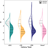 |
Fig. A.1. Distribution of the tidal index, Θ, for our galaxy samples divided into ‘central’ and ‘satellite’ sub-samples. The ‘central’ sample is shown on the right side (colour-filled), while the ‘satellite’ sample is shown on the left side (empty) of each violin plot. |
Appendix B: Distribution of galaxies in the TNG50-1 box
The distribution of our samples in the TNG50-1 box is shown in Fig. B.1. The UDGs, LSBs, HSBs, and the dwarfs are represented with ★, ▴, ▾, and ◼, respectively, following the same colour scheme as discussed in Sect. 3.1. Each of our samples are bordered with either yellow or orange colours - yellow for the isolated and orange for the tidally bound galaxies.
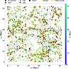 |
Fig. B.1. Distribution of the UDGs (★), LSBs (▴), HSBs (▾), and the dwarfs (◼) in the x-y plane of the TNG50-1 box. The isolated and tidally bound galaxies are represented with yellow and orange borders, respectively. The dots presented in grey scale represent the neighbouring galaxies in the TNG50-1 box. The variation in marker colour denotes the location of the galaxy on the z-axis (direction along the plane of the paper) - blue (black) denoting the nearest (∼ 0 Mpc) and green (fainter grey) denoting the farthest (∼ 50 Mpc comoving) galaxies of our sample (remaining in the box). |
Appendix C: Regression fitting coefficients
Slopes (m), intercepts (c), coefficients of determination (R2) and Spearman’s rank correlation coefficients (S) corresponding to each of the possible scaling relations for isolated (Iso) and tidally bound (Bound) subsets of the UDG, LSB, HSB and the dwarf samples obtained in Sect. 4.1 are enlisted in Table C.1. The p-values associated with R2 and S-coefficients are smaller than 0.05 in all cases except for the isolated UDGs and the isolated HSBs (denoted with *).
Values of m, c, R2 and S obtained in Sect. 4.1 for the UDGs, LSBs, HSBs, and dwarfs divided into isolated and tidally bound sub-samples.
All Tables
Values of m, c, R2 and S obtained in Sect. 4.1 for the UDGs, LSBs, HSBs, and dwarfs divided into isolated and tidally bound sub-samples.
All Figures
|
Fig. 1. Distribution of the TNG50-1 UDGs selected in our sample in the (left) Mg − Re, (middle) M* − Mdyn, and (right) M* − Mgas space marked in teal stars. To compare with the observed populations, the UDGs obtained from Leisman et al. (2017), Román & Trujillo (2017), Shi et al. (2017), Janowiecki et al. (2019), Marleau et al. (2021), Kadowaki et al. (2021), Poulain et al. (2022), and Jones et al. (2023) are superposed on the left panel. Similarly, on the middle and the right panel, the stellar, dynamical, and gas masses of the UDGs taken from Guo et al. (2020), Mancera Piña et al. (2020), Karunakaran et al. (2020), Marleau et al. (2021), Kong et al. (2022), and Kado-Fong et al. (2022) are shown for comparison. The teal dots represent the remaining UDGs identified in TNG50-1 while the grey dots denote the whole sample space from which the UDGs were selected. |
| In the text | |
|
Fig. 2. Distribution of the tidal index, Θ, for our galaxy samples. The UDGs are in teal, LSBs are in yellow, HSBs are in blue, and the dwarfs are in pink, along with their box plots. The blue region shows the buffer region that we rejected from our study. |
| In the text | |
|
Fig. 3. Histograms of (a) M*, (b) Mgas, (c) Mdyn, and (d) Mg of the UDGs, LSBs, HSBs, and the dwarfs considered in our study presented in teal, yellow, blue, and pink, respectively. The solid histograms represent the isolated galaxies, and the dotted histograms denote the tidally bound sub-samples. The medians of the isolated and tidally bound sub-samples are respectively denoted with solid and hollow triangles at the top of the panels using the same colour scheme. |
| In the text | |
|
Fig. 4. Possible scaling relations of (a) stellar-to-gas mass ratio versus gas mass (log10M*/Mgas vs. log10Mgas), (b) stellar-to-gas mass ratio versus total dynamical mass (log10M*/Mgas vs. log10Mdyn), and (c) total baryonic mass versus total dynamical mass (log10Mb vs. log10Mdyn). The UDGs, LSBs, HSBs, and the dwarfs are shown in teal, yellow, blue, and magenta colours, respectively. Each of the galaxy samples are divided into two sub-samples – isolated (denoted with filled circles) and tidally bound (denoted with empty circles). The scaling relations are obtained for the two sub-samples of each galaxy classes separately and plotted with solid and dashed lines, respectively. |
| In the text | |
|
Fig. 5. Distribution of the (top) intermediate-to-major axes ratios versus minor-to-major axes ratios ((b/a)DM–(c/a)DM) and (bottom) elongation and flattening (eDM − fDM) of the DM component of our galaxy samples. The histograms of the x and y data are plotted on the top and right sides of each panel, respectively, with equal bin widths, showing the fraction of galaxies in each bin. The isolated galaxies are shown with filled circles and filled histograms, while the empty circles and empty histograms represent the tidally bound sub-samples. The same colour scheme as in Fig. 4 is adopted. |
| In the text | |
|
Fig. 6. Distribution of the stellar component of our galaxy samples in (top) (b/a)*–(c/a)* and (bottom) e* − f* spaces. The plotting scheme is similar to Fig. 5. |
| In the text | |
|
Fig. 7. Distribution of the stellar component of our galaxy samples in T* − TDM space. The plotting scheme is similar to Fig. 5. |
| In the text | |
|
Fig. 8. Variation of (top) DM (βDM) and (bottom) stellar (β*) velocity anisotropy as a function of galactocentric radius normalised by the respective half-mass radius. Solid and dashed lines represent the median values of the isolated and tidally bound galaxy sub-samples, respectively. The 25th and 75th quartile regions are shown with shaded regions: solid-filled regions are for the isolated sub-samples and crossed diagonal lines are for the tidally bound ones. |
| In the text | |
|
Fig. 9. Variation of stellar (top) vertical-to-radial (σz/σr) and (bottom) tangential-to-radial (σθ/σr) velocity dispersion ratios as a function of galactocentric radius normalised by the stellar half-mass radius. The plotting scheme is similar to Fig. 8. |
| In the text | |
|
Fig. 10. Distribution of our galaxy samples in (top) the V/σ versus ϵ space and (bottom) the λRe versus ϵ space following the same plotting scheme as Fig. 5. The solid magenta line represents the predicted theoretical distribution of the axisymmetric galaxies with the anisotropy parameter βz = 0.7ϵ at an inclination of 90°, and dotted lines from right to left denote the theoretical distribution for decreasing inclinations. The leftmost dotted line corresponds to the face-on orientation. The grey dashed lines correspond to locations of galaxies at edge-on orientations with intrinsic ellipticities of ϵ = 0.85 − 0.35 (see Cappellari et al. 2007; Emsellem et al. 2007). |
| In the text | |
|
Fig. 11. Distribution of our galaxy samples in the (top) h3 and (bottom) h4 versus ratio of flux-weighted average of velocity and velocity dispersion (⟨V/σ⟩). A plotting scheme similar to that of the Fig. 5 has been adopted. |
| In the text | |
|
Fig. A.1. Distribution of the tidal index, Θ, for our galaxy samples divided into ‘central’ and ‘satellite’ sub-samples. The ‘central’ sample is shown on the right side (colour-filled), while the ‘satellite’ sample is shown on the left side (empty) of each violin plot. |
| In the text | |
|
Fig. B.1. Distribution of the UDGs (★), LSBs (▴), HSBs (▾), and the dwarfs (◼) in the x-y plane of the TNG50-1 box. The isolated and tidally bound galaxies are represented with yellow and orange borders, respectively. The dots presented in grey scale represent the neighbouring galaxies in the TNG50-1 box. The variation in marker colour denotes the location of the galaxy on the z-axis (direction along the plane of the paper) - blue (black) denoting the nearest (∼ 0 Mpc) and green (fainter grey) denoting the farthest (∼ 50 Mpc comoving) galaxies of our sample (remaining in the box). |
| In the text | |
Current usage metrics show cumulative count of Article Views (full-text article views including HTML views, PDF and ePub downloads, according to the available data) and Abstracts Views on Vision4Press platform.
Data correspond to usage on the plateform after 2015. The current usage metrics is available 48-96 hours after online publication and is updated daily on week days.
Initial download of the metrics may take a while.