| Issue |
A&A
Volume 707, March 2026
|
|
|---|---|---|
| Article Number | A330 | |
| Number of page(s) | 14 | |
| Section | Planets, planetary systems, and small bodies | |
| DOI | https://doi.org/10.1051/0004-6361/202556908 | |
| Published online | 20 March 2026 | |
Spatial variability of CH4 and C2H2 absorptions in Jupiter’s auroral regions from Juno-UVS observations
1
Laboratory for Planetary and Atmospheric Physics, STAR Institute, University of Liège, Liège, Belgium
2
Aix-Marseille Université, CNRS, CNES, Institut Origines, LAM, Marseille, France
3
Institute for Space Astrophysics and Planetology, National Institute for Astrophysics (INAF-IAPS), Rome, Italy
4
Southwest Research Institute, San Antonio, TX, USA
★ Corresponding author: This email address is being protected from spambots. You need JavaScript enabled to view it.
Received:
19
August
2025
Accepted:
5
February
2026
Abstract
Context. Ultraviolet (UV) auroral emissions on Jupiter offer a unique window into the coupling between the planet’s magnetosphere and upper atmosphere. Color ratios derived from molecular hydrogen emissions provide valuable diagnostics for the energy of precipitating electrons and the structure of the auroral atmosphere.
Aims. We aim to characterize the horizontal and vertical variability of hydrocarbon absorption in Jupiter’s auroral atmosphere using UV data from the Juno-UVS spectrograph and to investigate potential departures from the expected structure.
Methods. We constructed color ratio maps sensitive to CH4 and C2H2 absorptions for two of Juno’s close approaches to Jupiter, perijoves (PJs) 6 and 10, by integrating auroral H2 emission over hydrocarbon-sensitive spectral intervals. For CH4, we redefined the absorbed spectral band, replacing the traditionally used 125-130 nm interval with 135-140 nm to mitigate higher order calibration issues. In regions of intense auroral brightness, we developed a correction method to account for spectral distortion due to detector nonlinearities at high fluxes.
Results. The CH4 and C2H2 absorptions generally follow the expected vertical distribution, with the CH4 density extending to higher altitudes than C2H2. However, several localized regions show unexpected spatial distribution of the absorption. In PJ6, such anomalies are attributed to instrumental nonlinearities. Following the correction, the CR distributions become consistent with standard hydrocarbon vertical distributions. In PJ10, however, some anomalous patterns persist despite the correction. Spectral modeling studies indicate that these can be explained by modifying the relative abundances of CH4 and C2H2, suggesting horizontal compositional variability and possible deviations in the homopause altitude between species.
Conclusions. Our results confirm that hydrocarbon absorption in Jupiter’s aurora is vertically stratified, but that the altitude of this stratification itself varies horizontally with latitude and longitude. These findings underscore the importance of accounting for local atmospheric composition when interpreting UV auroral spectra and retrieving electron energy distributions. Juno-UVS thus provides a powerful diagnostic for probing both the auroral precipitation and upper atmospheric structure. The framework developed here enables more accurate retrievals of electron energies and provides new constraints on the spatial variability of Jupiter’s upper atmosphere. A systematic application to the full Juno dataset will offer deeper insights into the temporal and spatial dynamics of the Jovian aurora.
Key words: instrumentation: detectors / instrumentation: spectrographs / planets and satellites: atmospheres / planets and satellites: aurorae / planets and satellites: gaseous planets
© The Authors 2026
 Open Access article, published by EDP Sciences, under the terms of the Creative Commons Attribution License (https://creativecommons.org/licenses/by/4.0), which permits unrestricted use, distribution, and reproduction in any medium, provided the original work is properly cited.
This article is published in open access under the Subscribe to Open model. This email address is being protected from spambots. You need JavaScript enabled to view it. to support open access publication.
1 Introduction
Jupiter’s auroral emissions mostly originate from the precipitation of energetic electrons that have been accelerated within the planet’s magnetosphere. Upon entering the upper atmosphere, these electrons collide with atmospheric constituents, leading to excitation, dissociation, and ionization processes that generate characteristic ultraviolet (UV) emissions. As such, auroral emissions offer a remote diagnostic of magnetospheric dynamics and provide key insights into the physical mechanisms responsible for electron acceleration.
The first UV detection of Jovian aurorae was achieved during the Voyager 1 flyby, which revealed emissions from both atomic hydrogen (Lyman-α) and molecular hydrogen (H2) bands, specifically the Lyman ( ) and Werner (C1Πu → X1∑g+) transitions (Broadfoot et al. 1979). This discovery marked the beginning of several decades of continuous monitoring, notably by the International Ultraviolet Explorer (IUE), which provided valuable temporal coverage and spectral information (Clarke et al. 1980; Livengood 1992; Gladstone & Skinner 1989; Harris et al. 1996).
More recently, UV observations conducted with the Hubble Space Telescope (HST) have considerably enhanced our understanding of the aurora. Imaging instruments such as the Faint Object Camera (FOC) and the Wide Field and Planetary Camera 2 (WFPC2) have offered high-resolution views of auroral morphology (Dols et al. 1992; Gérard et al. 1994; Prangé et al. 1998; Clarke et al. 1996, 1998; Grodent et al. 1997), while the Space Telescope Imaging Spectrograph (STIS) has provided complementary spectroscopic diagnostics (Gustin et al. 2002). Despite the wealth of data collected, the spatial and temporal complexity of Jupiter’s auroral structures continues to pose challenges to compiling a complete characterization (Grodent 2015). Nonetheless, these observations have enabled a general classification of the main auroral components: a bright, partially closed main emission, dynamic emissions located poleward of this structure, and equatorward features including the auroral footprints of the Galilean moons: Io, Europa, and Ganymede.
Beyond the spatial morphology, spectroscopic measurements provide a powerful means of probing the energy of the precipitating electrons responsible for auroral emissions. In particular, the color ratio (CR) has proven to be a robust diagnostic for constraining the depth of electron penetration into Jupiter’s upper atmosphere.
The CR exploits the wavelength-dependent absorption of H2 emissions by atmospheric hydrocarbons, primarily methane (CH4). It is defined as the ratio of auroral brightness in a weakly absorbed spectral interval over that measured in a strongly absorbed interval. The most optimal definition of this ratio uses sufficiently wide bands with high signal, with close to no absorption for the numerator and strong absorption for the denominator. Theoretically, the earliest formulation of the color ratio (Yung et al. 1982) fits all these requirements. It is defined as
 (1)
(1)
The denominator was however later refined to 125-130 nm to avoid contamination by the instrumentally broadened Lyman-α line when using the Juno UltraViolet Spectrograph (Juno-UVS; Gérard et al. 2019). The currently adopted form is
 (2)
(2)
The CR can also be adapted to meet specific requirements. Alternative formulations of the CR can be used to probe the influence of other hydrocarbons. For example, to probe C2H2 absorption, we define
 (3)
(3)
where the 150-153 nm interval is particularly sensitive to C2H2. Additionnally, for instruments with limited spectral coverage at longer wavelengths, such as Hisaki/EXCEED (which extends only up to 148 nm), a modified ratio can be adopted. Tao et al. (2016) define CRexceed as
 (4)
(4)
where the chosen bands ensure differential CH4 absorption, avoid H2 self-absorption and fall within the instrument’s sensitivity range. This example illustrates how the CR framework can be adapted to different spectral instruments, while retaining its diagnostic value.
The CH4 color ratio provides a physically meaningful diagnostic because CH4 is confined below the homopause, which is the transition altitude between molecular diffusion and eddy diffusion. Below this level, heavier hydrocarbons are well-mixed due to turbulent mixing; above it, molecular diffusion dominates and their densities drop off sharply with altitude. Auroral H2 emissions generated above the homopause (by low-energy electrons) undergo very slight absorption, whereas emissions produced deeper in the atmosphere (by higher-energy electrons) are increasingly attenuated by CH4. Consequently, a higher CR
indicates deeper penetration of energetic particles and, thus, a higher characteristic electron energy.
A quantitative link between the CR and the characteristic energy of precipitating electrons has long been exploited as a remote sensing tool to constrain electron penetration depths in planetary aurorae (e.g., Trafton et al. 1994; Grodent et al. 2001; Gustin et al. 2002, 2016; Ajello et al. 2005; Gérard et al. 2014). This technique relies on the fact that CH4 resides predominantly below the homopause, so that increasing absorption in CH4-sensitive spectral bands reflects deeper energy deposition and, thus, higher energy electrons. The CR offers a relationship with the characteristic energy E0 of precipitating electrons, provided the emission geometry is fixed.
Building on this established principle, Benmahi et al. (2024a) presented a refined version of the CR—E0 relationship using the TransPlanet (Lilensten et al. 1989) electron transport model. This model combines electron transport and H2 excitation with detailed UV emission modeling through a hydrocarbon-rich atmosphere and includes the effect of photon emission angle, which modulates the atmospheric path length and, thus, the probability of absorption along the line of sight. By simulating auroral emissions for both monoenergetic and kappa electron energy distributions and computing the corresponding synthetic CRs, a calibration curve is derived, which can be inverted to estimate E0 from observed CRs.
Compared to in situ particle measurements from instruments such as JADE and JEDI onboard Juno, this spectroscopic method offers two main advantages. First, UVS spectro-imaging provides much broader spatial and temporal coverage than pointsampling particle detectors, enabling a global view of auroral precipitation. Second, in situ instruments sometimes probe electrons above the acceleration region (~1-2 RJ, where RJ is Jupiter’s equatorial radius, 71 492 km) and might not reflect their energy at atmospheric impact. The spectroscopic approach, in contrast, diagnoses the actual energy deposition in the upper atmosphere and, thus, it can more directly constrain the energy of the precipitating electrons, but with a strong reliance on models and assumptions.
This spectroscopic method, though powerful, inherently depends on the assumed vertical and horizontal distribution of CH4 in the atmosphere. In particular, any variation in the altitude of the homopause (above which CH4 is strongly depleted) can significantly impact the absorption depth of UV photons and, thus, bias the energy retrieval from CR measurements (Benmahi et al. 2024b).
Previous studies have shown that Jupiter’s auroral hydrocarbons density profiles show variations both vertically and horizontally. For instance, infrared (IR) observations, particularly from Juno and ground-based telescopes, have revealed vertical variability up to 100 km in the altitude of CH4 and other hydrocarbons across Jupiter’s auroral regions (Sinclair et al. 2017, 2018, 2020, 2025). In particular, variations in the altitude of the CH4 homopause have been observed, reaching up to 100 km between the regions poleward and equatorward of the main emission (Sinclair et al. 2025). UV color-ratio mapping with Juno/UVS also highlighted spatial structures in auroral emissions: Greathouse et al. (2021) identified two distinct CR regimes in the northern polar region: a high-CR “swirl region” and a lower-CR collar, both strongly controlled by the orientation of the magnetic dipole. They discuss the fact that the variation of these CRs cannot always be explained by different precipitation energy and could also be linked to changes in the atmospheric composition or geometry. Solar-reflected UV measurements have further expanded this picture. Giles et al. (2023) showed that the depth and shape of the C2H2 absorption band vary significantly across Jupiter’s south pole, revealing a localized enhancement within the auroral oval, where C2H2 abundances are ~3× higher than in adjacent longitudes. These results established that hydrocarbon abundances are not uniform, while also demonstrating that UV absorption features have the capacity to diagnose horizontal composition gradients. Recent JWST observations provide a more detailed view of this complexity. In the south, Rodríguez-Ovalle et al. (2024) found elevated temperatures at two pressure levels (0.01 and 1 mbar), an auroral homopause raised up to ~590 km compared to 350-460 km elsewhere and divergent spatial distributions of C2H2 and C2H6; the former is enhanced inside the oval, while the latter increasing smoothly toward the rotational pole. In the north, Melin et al. (2025) mapped CH4 and H3+ emission with NIRSpec, showing rapid temperature variability and CH4 emission along the main oval, likely linked to direct precipitation. They proposed that CH4 band ratios could constrain penetration depth, mirroring the physical principle behind UV color ratios. These compositional gradients likely result from magnetospheric particle precipitation, which alters both the chemical composition (Sinclair et al. 2019, 2023; Benmahi et al. 2020; Cavalié et al. 2023) and thermal structure (O’Donoghue et al. 2021) of the upper atmosphere (see Hue et al. (2024) for a comprehensive review). Together, these studies show that hydrocarbons density gradients are not only vertical: their altitude, abundance, and relative composition vary with latitude and longitude.
Since the CR depends critically on the amount of CH4 encountered by auroral photons (i.e., on the depth at which UV emissions are absorbed), such variability directly affects the inferred energy of precipitating electrons. For high-energy electrons, which deposit their energy deeper in the atmosphere, a higher homopause leads to increased absorption and thus a higher CR, potentially resulting in an overestimate of the characteristic energy, E0, if it is not properly accounted for. Conversely, a lower homopause altitude leads to less CH4 absorption and may cause an underestimation in terms of E0.
This effect can introduce systematic uncertainties of up to 200 keV in the inferred energies of the most energetic auroral electrons, as shown in Benmahi et al. (2024b). Therefore, any attempt to retrieve accurate particle energy distributions from CR measurements must take into account the horizontal variability of CH4 and the vertical structure of the atmosphere. This characterization motivates the present work, where we seek to refine hydrocarbon absorption diagnostics in Juno-UVS data, apply them to PJ6 and PJ10, and reveal new insights into the spatial distribution of CH4 and C2H2 in Jupiter’s auroral atmosphere.
2 Instrumentation and models
2.1 The Juno mission and the UVS instrument
The Juno spacecraft, part of NASA’s New Frontiers program, entered orbit around Jupiter on 4 July 2016 following its launch in 2011. The mission’s primary objectives include probing Jupiter’s internal structure, magnetic and gravitational fields, atmospheric composition, and dynamics, as well as investigating the nature and drivers of its auroral emissions (Bolton et al. 2017; Bagenal et al. 2017).
To fulfill these goals, Juno was placed on a highly elliptical polar orbit designed to minimize radiation exposure while enabling close approaches to the planet. Each orbit, referred to as a perijove (PJ), brings the spacecraft within approximately 4200 km of the cloud tops and extends out to over 100 RJ at apoapsis.
Among Juno’s nine scientific instruments is UVS, a key tool for auroral studies, comprising a far- and extreme-UV (FUV-EUV) spectrograph covering the 68-210 nm range (Gladstone et al. 2017). It uses a flat scanning mirror to direct incoming photons toward a primary mirror and a dogbone-shaped slit, composed of two wide segments at the ends (0.2°× 2.5°) and a narrower central segment (0.025°× 2.0°). Light passing through the slit is dispersed by a diffraction grating and detected on a two-dimensional (2D) sensor.
The spin-stabilized spacecraft completes one rotation every ~30 seconds, allowing UVS to sweep across the auroral regions and build up spatial coverage. Each rotation yields spectrally resolved photon counts associated with wavelength, time, and emission angle. The UV emissions observed by UVS primarily originate from atomic hydrogen (Lyman-α) and H2 transitions in the Lyman and Werner bands. These features result from electron-impact excitation of the upper atmosphere and provide critical diagnostics of auroral processes. For this study, we used UVS observations to investigate spectral and energetic characteristics of Jupiter’s aurora.
2.2 Atmospheric model: Grodent et al. (2001)
The structure of the auroral atmosphere assumed in this study is based on the 1D model described by Grodent et al. (2001). This model provides vertical profiles for the major neutral species in Jupiter’s upper atmosphere (H, H2, He, CH4, and C2H2) from the tropopause (near 100 mbar, approximately 50 km above the visible cloud tops) to the upper thermosphere (10−9 mbar, or about 2300 km altitude). Hydrogen (both molecular and atomic) and helium are present at all altitudes, while CH4 and C2H2 are mostly confined below the homopause.
The adopted model assumes a horizontally homogeneous atmosphere, which is a simplification. As discussed in the introduction, IR observations have revealed significant variability in the altitude of the CH4 homopause across auroral latitudes, which can impact the reliability of CR-based energy diagnostics. Despite this limitation, the Grodent et al. (2001) model remains widely used in auroral studies due to its physical consistency and compatibility with codes such as TransPlanet and it provides a reasonable baseline for investigating first-order effects in the auroral regions.
2.3 Electron transport and emission: TransPlanet
To simulate electron precipitation and the resulting UV emissions in Jupiter’s auroral atmosphere, we used the TransPlanet electron transport model. Originally developed by Lilensten et al. (1989), this model has since been adapted to various planetary environments, including studies of Jupiter’s auroral regions and the interaction between Triton’s atmosphere and Neptune’s magnetosphere (Benmahi 2022; Benmahi et al. 2024a,b; Benne et al. 2024). TransPlanet also includes a dedicated UV emission model to compute H2 emissions in the 80-210 nm range generated by excitation from precipitated magnetospheric electrons collisions with Jupiter’s atmosphere (Benmahi et al. 2024a,b).
TransPlanet solves the Boltzmann equation for each altitude bin for a suprathermal electron population precipitating into a model atmosphere. The equation accounts for both elastic and inelastic collisions with atmospheric species, including the production of secondary electrons. The Jovian atmospheric profile used is based on Grodent et al. (2001).
After solving the transport problem, the resulting altitudedependent electron energy flux is used as input for the UV emission model, which calculates the excitation and subsequent radiative de-excitation of H2 molecules. This process produces UV emissions primarily in the Lyman and Werner bands. The UV emission model includes direct excitation, cascade contributions and self-absorption effects, with photon redistribution toward lower-energy transitions (Benmahi et al. 2024a). Absorption by hydrocarbons such as CH4, C2H2, and C2H6 is also incorporated to yield realistic spectra. This UV emission model has been validated by Benmahi et al. (2024a) against laboratory data, notably the electron-impact excitation spectra of H2 from Liu et al. (1995), showing good agreement in line positions and relative intensities.
The final output from TransPlanet includes the total vertical energy flux profile of precipitating electrons and a synthetic UV spectrum by H2. This model spectrum serves as a basis for the comparison with UVS observations presented in Sect. 4.1.
3 Data processing and method
3.1 Spectral cubes
We constructed spectral cubes for PJ6 and PJ10 using the same method described in Benmahi et al. (2024a). The input data consist of time-tagged photon lists recorded by UVS, which scans the sky as the spacecraft spins, enabling coverage of Jupiter’s auroral regions in the FUV range (Bonfond et al. 2017). Each detected photon is associated with ancillary parameters such as its time of detection, wavelength (from detector position), detector coordinates (x, y), emission angle, and the corresponding projected location on Jupiter in System III coordinates (latitude and longitude), derived from the spacecraft’s orientation and the instrument’s pointing geometry (Acton et al. 2018; Acton 1996).
Photon counts are converted into physical units of spectral flux using the instrument’s effective area, which is determined from regular stellar calibration observations performed throughout the mission (Hue et al. 2021, 2018; Greathouse et al. 2013). To ensure consistent spectral resolution and maximize the S/N, only photons collected through the two wide slits of UVS are retained for analysis. These wide slits offer a spectral resolution of approximately 2.1 nm (Greathouse et al. 2013).
The calibrated photon lists are then binned into threedimensional (3D) spectral cubes defined over latitude, longitude (both in System III), and wavelength. The spatial grid is sampled every 1° in latitude and longitude. In the spectral dimension, we adopted a sampling of 0.1 nm, which satisfies the Nyquist criterion based on the UVS spectral point spread function. Photons are accumulated over selected time intervals. The resulting cubes span the 125-170 nm range and provide spatially and spectrally resolved maps of the auroral emission for each hemisphere.
From the spectral cubes, we derived brightness maps of Jupiter’s northern and southern auroral regions. In particular, we computed H2 emission maps by integrating the flux over the 155-162 nm wavelength band, which is minimally affected by hydrocarbon absorption and corresponds to the strongest Lyman and Werner band emissions. These maps reveal the large-scale morphology of the auroral emissions, including specific features such as the main emission, polar emissions, and transient features such as dawn storms or injection signatures.
Figure 1 shows the H2 brightness maps obtained during PJ6 (from 2017-May-19 01:01:05 UTC to 2017-May-19 10:39:48 UTC) and PJ10 (from 2017-Dec-16 13:45:18 UTC to 2017-Dec-16 22:57:00 UTC) for the southern pole. The main auroral emission appears as a bright arc encircling the pole, while all the emissions contained inside of the main emission are called the polar emissions. The emissions outside of the main emission contain signatures of injections as well as the footprints of the Jovian satellites.
The spectral cubes also enable the construction of hydrocarbon absorption maps based on CRs. In particular, we aim to compare the absorptions by CH4 and by C2H2, two hydrocarbons that dominate the optical depth in distinct UV intervals. Each CR is defined as the ratio of the integrated H2 brightness in an unabsorbed spectral band to that in a hydrocarbon-sensitive absorption band.
These ratios allow us to isolate the contribution of each hydrocarbon species. Figure 2 illustrates the spectral intervals used for the CR calculations: panel a shows a simulated unabsorbed H2 spectrum from TransPlanet, with absorption bands indicated, while panel b, from Benmahi et al. (2024a), displays the optical depth for CH4 and C2H2 highlighting the same spectral ranges. In the absence of strong dynamical or chemical perturbations, CRCH4 and CRC2H2 maps are expected to exhibit similar morphologies. This expectation is justified because both CH4 and C2H2 are primarily located below their respective homopauses, where molecular diffusion is slow and advective transport dominates, leading to comparable spatial distributions.
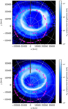 |
Fig. 1 Southern auroral H2 brightness maps integrated over the 155162 nm unabsorbed band for two perijoves: (a) PJ6 and (b) PJ10. |
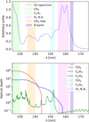 |
Fig. 2 Spectral diagnostics for hydrocarbon absorption and CR computation. Transparent green and cyan bands indicate the absorption spectral ranges used for CR calculations (125-130 nm for CH4, 150153 nm for C2H2), while the magenta band represents the nonabsorbed region assumed to be free of hydrocarbon absorption. The orange band is the new spectral range proposed for absorption of CH4 and the purple one is used to scale the color ratio in case of detector nonlinearity in the unabsorbed band (see Sect. 3.3). Upper panel: Simulated unabsorbed H2 spectrum from TransPlanet in dark blue. Lower panel: Corresponding optical depth for CH4, C2H2, and C2H6, showing the ranges used in CR calculations (from Benmahi et al. 2024a). |
3.2 Detector response at high flux levels
The photon detection process is characterized by the pulse height distribution (PHD), which characterizes the distribution of output signal amplitudes generated by photoelectron avalanches in the microchannel plates (MCPs) of the UVS detector (Hue et al. 2018; Greathouse et al. 2013). When a UV photon strikes the photocathode, it ejects a photoelectron that initiates a cascade of secondary electrons within the MCP channels. Each such cascade results in an electronic pulse and the amplitude (height) of these pulses depends on several factors, including gain uniformity, electron multiplication statistics, and the intrinsic variability of the MCP.
A PHD that is shown as a unimodal distribution centered at above a typical amplitude is indicative of stable gain and reliable photon counting. However, when observing very bright regions or when using instrumental configurations that increase the incoming flux (e.g., the wide slit), the PHD can become distorted. This distortion results in a shift of the peak to lower pulse heights and a broadening or flattening of the distribution. In practice, such degraded PHDs are indicative of lower detector gain, resulting in fewer detected photons. This effect is illustrated in Fig. 3, where we compare two PHDs recorded during the PJ10 flyby over the same auroral region: one in the 135-140 nm interval, yielding a normal PHD with a peak above 5 (which is the acceptable threshold) and one in the 125-130 m band, where the PHD is significantly degraded with the peak falling below the acceptable threshold.
This instrumental effect is spectrally dependent. Before constructing the CR maps, we assessed the reliability of the PHD in different spectral intervals. The detector regions receiving the highest photon flux (e.g., those associated with the Lyman-α line and the unabsorbed band: 155-162 nm) are the most susceptible to high flux-induced distortion of the PHD.
The commonly used CH4 absorption band at 125-130 nm lies close to the intense Lyman-α emission, which is known to suffer from instrumental scrubbing causing gain sag. To assess the impact of this effect, we performed a PHD analysis for the 125-130 nm range, the results of which are presented in Appendix A. This analysis shows that, in many regions, the PHD peak falls below the critical threshold of 5, indicating that the detector response deviates from the nominal calibration and that the corresponding measurements are likely unreliable.
The 155-162 nm interval, which corresponds to the unabsorbed region of the spectrum also typically exhibits high photon fluxes. In a particularly bright region of PJ6 corresponding to a dawn storm, we extracted two representative spectra. As shown in Fig. 4, the wide slit observation displays a strong flattening of the H2 emission continuum between 155-162 nm, suppressing the expected double-peaked structure characteristic of this unabsorbed spectral interval. In contrast, the spectrum from the narrow slit retains its expected shape, due to lower fluxes via the narrow slit.
These regions of high brightness show both spectral distortions and degraded PHDs, with the peak falling below a value of 5. This shift toward lower pulse amplitudes is consistent with the detector’s high flux nonlinearity, likely caused by high photon count rates exceeding the local charge recovery capability of the microchannel plate. As a result, photon events are underamplified, leading to gain suppression and spectral flattening, which could be mistakenly ascribed to atmospheric absorption. The detailed PHD analysis for the 155-162 nm range is presented in Appendix B.
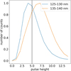 |
Fig. 3 Comparison of normalized PHDs in the 125-130 nm spectral band (blue) and the 135-140 nm spectral band (orange) during PJ10 for the region between 70°S and 73°S and between 30°W and 60°W. The orange histogram (135-140 nm) shows a well-calibrated distribution with a peak above 5. The blue histogram (125-130 nm) shows a PHD with a degraded shape and a peak below 5, indicating significant signal loss. |
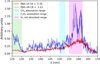 |
Fig. 4 Comparison between a spectrum affected by instrumental flattening (red) and an unaffected spectrum (blue), both extracted from the same auroral region during PJ6. The affected spectrum, observed with the wide slit in a very bright area, exhibits a flattened shape with missing emission features particularly in the unabsorbed band. In contrast, the narrow-slit spectrum in the same region clearly shows the characteristic double-peaked H2 continuum around 160 nm. |
3.3 Corrections for high flux-induced calibration issues
We want to find ways to create color ratio maps, while avoiding the spectral and spatial regions where the high fluxes compromise the detector. The objectives are preserving the diagnostic power of the color ratio and using spectral bands with the highest possible fluxes, while maintaining reliable photon counting.
The 125-130 band very often displays a degraded PHD due to its proximity to the Lyman-alpha band on the detector. To mitigate the impact of these calibration issues on the 125-130 band, we chose to change the absorbed band used in the CH4 CR calculation. We selected the 135-140 nm interval as a more robust alternative (see Figs. 2 and 3), which remains within the CH4 absorption range but is less affected by instrumental artifacts. A more detailed insight into the choice of this new interval is provided in Appendix A.
Accordingly, we adopted the revised definition,
 (5)
(5)
in place of Eq. (2).
In contrast to the absorbed band, which experiences an almost systematic effect, the unabsorbed band (155-162 nm) is subject to calibration issues only for very bright events. To address this, we developed a correction scheme (Appendix B) that detects and adjusts CR values only in regions affected by detector high-flux nonlinearity. In these regions, we also observed a flattening of the spectrum in the unabsorbed band. By comparing the intensities of two narrow diagnostic bands within the unabsorbed part of the H2 spectrum, we identified the regions where that spectrum is flattened. The ratio between band A (157-158.5 nm), which contains a sharp emission peak highly sensitive to spectral flattening and band B (163-165 nm), a nearby continuum region largely immune to nonlinearity effects will become smaller when the spectrum is flattened. Pixels where the observed A/B ratio falls significantly below the theoretical value from TransPlanet simulations are flagged as degraded and their unabsorbed-band flux is reconstructed from band B using the theoretical ratio, allowing the CH4 and C2H2 CRs to be corrected accordingly.
In the regions where A/B falls under a certain treshold, the corrected CH4 and C2H2 CRs are computed using the following formulas:
 (6)
(6)
 (7)
(7)
Here, CH4 CR is not affected as much by this instrumental effect. Indeed, the 135-140 nm range lies in a part of the detector that generally receives low local fluxes because H2 emissions are intrinsically weaker there and also because they are further attenuated by CH4 absorption. When the emission in the CH4 absorption band (135-140 nm) is strongly absorbed, the spectrum nearly flattens in this interval, leading to a very high CR, whatever the intensity of the emission in the unabsorbed range. This CR is thus minimally impacted by the flattening of the spectrum. Consequently, the conclusions drawn from CH4 CR maps regarding hydrocarbon absorption largely hold.
In contrast, the 150-153 nm range used for C2H2 absorption lies within a spectral region (150-165 nm) where H2 emissions are much stronger. Here, high local count rates occur across both the absorbed and unabsorbed portions of the spectrum, making the C2H2 CR much more sensitive to detector nonlinearities. These effects in the unabsorbed range can then artificially lower the C2H2 CR, even when substantial absorption is present in the 150-153 nm interval. As a result, the corrected CR values provide a more accurate diagnostic of hydrocarbon absorption in high-brightness auroral zones.
3.4 Modeling the CR-energy relationship with TransPlanet
To interpret the revised CH4 CR as a diagnostic of precipitating electron energy, we derived an empirical relationship between the CR and the characteristic energy, E0, of the electron distribution. Our approach follows the methodology developed by Benmahi et al. (2024a), who established a 2D functional dependence CR(E0, θ) using the TransPlanet code.
In our case, we applied this same method to the newly adopted CH4 CR (Eq. (5)). We simulated H2 auroral emission spectra using TransPlanet for both monoenergetic and kappatype electron energy distributions, over a grid of E0 values and emission angles, θ, (from 0° to 80°). Each spectrum was convolved with the Juno-UVS instrument line-spread function and the CR was computed accordingly. Following the formalism proposed by Benmahi et al. (2024a), the CR-energy-angle relationship was fitted using the following analytical expression,
![Mathematical equation: \begin{align}\text{CR}(E_0, \theta) =\& \left[A \cdot \left(\tanh\left(\frac{E_0 - E_c}{B \cdot (1 - C \cdot \sin(\theta))}\right) + 1\right)\right.\label{eq:cr_model} \\[-0.2em]& \left. \cdot \log\left(\left(\frac{E_0}{D}\right)^{\alpha} + e\right)^{\beta}\right] \notag\\[-0.2em]& \cdot \left[1 + \delta \cdot \left(\sin(\theta)\right)^{\gamma / (E_0 / 1.5 \times 10^5)}\right], \notag\end{align}](/articles/aa/full_html/2026/03/aa56908-25/aa56908-25-eq9.png) (8)
(8)
where E0 is the characteristic electron energy (in eV), θ is the emission angle, A is the amplitude scaling factor, Ec is a threshold energy (in eV), B and C modulate the smoothness and angular sensitivity of the tanh transition, D, α, and β define the logarithmic energy growth at high energies, δ and γ account for angular modulation at high energies, and e is Euler’s number, ensuring continuity at low energy. The fitting procedure uses a Markov chain Monte Carlo (MCMC) optimization with the emcee sampler (Foreman-Mackey et al. 2013), using 250 walkers and 2500 iterations to ensure convergence.
The best-fit parameters for Eq. (8) were determined separately for the northern and southern hemispheres and for both mono-energetic and kappa-type distributions, since the CR-energy relation depends explicitly on the magnetic dip angle, which differs between the two hemispheres. These parameters are summarized in Table 1 for the northern auroral region and Table 2 for the southern counterpart. The model is valid over the characteristic energy range of approximately 50 eV to 150 keV and across the magnetic latitudes covered by the auroral emissions.
Fit parameters for the CR-energy relationship in the northern hemisphere.
Fit parameters for the CR-energy relationship in the southern hemisphere.
4 Results
After applying the corrections detailed in Sect. 3.3, we built color ratio maps for both CH4 and C2H2 using Eqs. (5) and (3), respectively, for PJ6 and PJ10 for the southern aurora. The choice of these PJs is motivated by the color ratio maps that were produced before correction that are displayed in Appendix C. For both PJs, the absorption by CH4 and C2H2 are not consistent with each other in the uncorrected maps. From the vertical structure of the atmosphere, we assumed the spatial distribution of the color ratios to be correlated.
4.1 Perijove 6
Figure 5 illustrates the outcome of applying the spectral flattening correction to PJ6. The correction restores CR values that are coherent with those predicted by our reference atmospheric model (Grodent et al. 2001). This supports the idea that that the uncorrelated distributions of CH4 and C2H2 are not atmospheric in nature, but that they originated instead from instrumental effects linked to high flux nonlinearity detector effects.
4.2 Perijove 10
The same spectral flattening correction method was applied to PJ10 to assess whether the CR anomalies identified in the initial CR maps could be attributed to detector-induced effects. Pixels were flagged as saturated using the same diagnostic A/B ratio criterion and corrected CR maps were produced. As illustrated in Fig. 7, these corrected maps exhibit only minor differences compared to the original, uncorrected ones (Figs. C.2a and C.2b). This indicates that the apparent discrepancies between CH4 and C2H2 absorption features in PJ10 are not instrumental in origin.
Unlike PJ6, where the anomalous horizontal distribution of the CRs was fully resolved after correction, the persistent CR anomalies in PJ10 suggest a physical, rather than an instrumental, cause. These features could reflect real horizontal or vertical variations in hydrocarbon distributions, possible changes in the local atmospheric structure such as temperature, or mixing ratios. This result underscores the necessity of correcting for instrumental effects before interpreting spectral morphologies and points to a potential deviation from the atmospheric model in the auroral regions of PJ10.
5 Discussion
The results of this study validate the methodological advances introduced to improve hydrocarbon absorption diagnostics in Juno-UVS data. Redefining the CH4 CR with the 135-140 nm interval yields robust results that are consistent with observational trends in nonsaturated regions, while being less affected by instrumental artifacts than the traditional 125-130 nm band. It is worth noting that the qualitative interpretation of color-ratio maps in previous studies remains valid, as the overall morphology of the CH4 color ratio maps is only marginally affected by the change in the absorbed spectral interval. In parallel, the correction method applied to the unabsorbed 155-162 nm range restores reliable CR maps in high-brightness regions in PJ6 by identifying saturated pixels via the A/B band ratio (Appendix B) and mitigating nonlinearity effects related to the detector. This analysis further reveals that the brightness of H2 emission in the 155-162 nm band has been systematically underestimated in regions of highest flux, such as dawn storms (Bonfond et al. 2021). For example, the power of the PJ6 dawn storm was underestimated by approximately 10%.
However, despite the success of these corrections in PJ6, significant CR anomalies remain in PJ10. To assess their origin, we selected two polygonal regions (see Fig. 7), each exhibiting contrasting behaviors: one with high CH4, but low C2H2 CR and another with the opposite trend. For each polygon, we computed the average spectrum to evaluate whether these anomalies reflect genuine atmospheric structure.
Using the TransPlanet electron transport model, we simulated the FUV auroral spectra resulting from a kappa-distributed population of precipitating electrons passing through the Jovian atmosphere, using the Grodent et al. (2001) atmospheric reference model. The emission angle and mean electron energy for each simulation were fixed based on the median values derived from the data for each polygon and the CR(E0) relationship. We explored the sensitivity of the modeled spectra to changes in atmospheric composition by applying simple multiplicative adjustment factors (FCH4, FC2H2, FC2H6) to the vertical hydrocarbon profiles. This approach is intended as a proof of concept, rather than a formal inversion.
In the region with a high CH4 CR and mild C2H2 CR (see Fig. 7 left panel), the best fit (see Fig. 9) was obtained with adjustment factors of FCH4 = 2.0, FC2H2 = 0.3, and FC2H6 = 0.4. These values suggest a local enhancement of CH4 and a depletion of C2H2 compared to the reference atmosphere, consistent with the observed uncorrelated CRs. In contrast, for the second region (Fig. 7 right panel), where the CH4 CR is mild and the C2H2 CR is high, the best fit (see Fig. 9) was obtained with FCH4 = 1.0, FC2H2 = 1.0, and FC2H6 = 1.0, consistent with the nominal composition.
This exploratory fitting exercise shows that the anomalous spectral signature observed in PJ10 cannot be reproduced by known instrumental effects, such as detector nonlinearity at high flux. Matching the observed spectra requires substantial departures from the nominal hydrocarbon profiles (particularly an enhanced CH4 abundance and a depleted C2H2 column), indicating genuine horizontal variability in auroral composition. Because this procedure does not involve a formal retrieval or statistical exploration of parameter space, the inferred scaling factors should be viewed as indicative rather than definitive. A rigorous inversion, including error bars and parameter correlations, is beyond the scope of this work and will be addressed in future studies.
Our results therefore suggest genuine horizontal heterogeneities in auroral hydrocarbon abundances. This interpretation aligns with previous Juno-UVS solar reflection observations (Giles et al. 2023) and ground-based mid-infrared measurements (Sinclair et al. 2017, 2018, 2020, 2025), which revealed horizontal variability in CH4 and C2H2 homopauses. Using recent JWST measurements, Rodríguez-Ovalle et al. (2024) and Melin et al. (2025) also report elevated homopauses, strong temperature gradients, and distinct spatial patterns in C2H2 and C2H6 abundances. Solar-reflected UV observations from Juno/UVS (Giles et al. 2023) similarly revealed longitudinal variations in C2H2 absorption at the south pole, demonstrating that hydrocarbon abundances are not zonally symmetric. Our results add to these previous works by identifying localized variations of the color ratios of CH4 and C2H2 within the main auroral emission region.
The different observational techniques used so far to probe Jupiter’s upper atmosphere reach different pressure and altitude ranges, which explains why they do not always agree or trace the same atmospheric processes. The IR thermal spectroscopy (with CIRS, TEXES or JWST/MIRI) primarily senses the stratosphere at pressures from ~10 mbar down to ~10−3-10−4 mbar, constraining hydrocarbon abundances, aerosols, and temperature. The NIR auroral observations with JWST/NIRSpec, based on H3+ and CH4 emissions, probe much lower pressures in the thermosphere, typically ≲10−6-10−8 mbar (Melin et al. 2025). Solar-reflected UV observations (e.g., Giles et al. 2023) probe the absorption of solar photons in the upper stratosphere and near the homopause, typically around ~10-2-10−4 mbar. In contrast, auroral UV color-ratio diagnostics (as those used here) are sensitive to the hydrocarbon column above the H2 emission layer, which corresponds to pressures of roughly ~10−5 down to ~10−7 mbar for characteristic electron energies of ~1-100 keV. As a consequence, CR anomalies reveal not only compositional but also structural vertical changes (homopause altitude, vertical mixing, and energy deposition depth), making them a critical complement to IR and reflected-UV diagnostics.
Possible drivers of this variability include auroral-induced chemistry from electron precipitation, which can locally alter hydrocarbon abundances (Sinclair et al. 2019, 2023; Hue et al. 2024), combined with atmospheric transport through winds or vertical mixing, redistributing species laterally (Hue et al. 2024). Both processes affect the homopause altitude, which strongly influences UV absorption and, thus, the observed CRs.
The detection of robust, localized CR anomalies not attributable to instrumental effects demonstrates the diagnostic potential of CR maps beyond energy retrieval. In addition to constraining electron precipitation, they provide insights into atmospheric composition and dynamics, acting as tracers of both energy deposition and the atmospheric response to magnetospheric forcing.
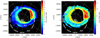 |
Fig. 5 CR maps for PJ6 in the southern auroral region after applying the corrections presented in Sect. 3.3. Right panel: CR map for CH4. Left panel: CR map for C2H2. The corrected regions are highlighted in Fig. 6. |
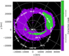 |
Fig. 6 Mask map showing the correction applied to CR maps of PJ6. The purple pixels have not been corrected and the green ones have been replaced by the corrected CRs (Eqs. (6) and (7)). |
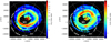 |
Fig. 7 CR maps for PJ10 in the southern auroral region after applying the corrections presented in Sect. 3.3. Right panel: CR map for CH4. Left panel: CR map for C2H2 The corrected regions are highlighted in Fig. 8. A region centered near 85°S, 180°W exhibits strong CH4 absorption but weak C2H2 absorption, while an opposite pattern (low CH4 and enhanced C2H2 absorption) is observed around 70°S, 30°W. Dashed white polygons outline regions with contrasting CR behaviors. |
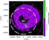 |
Fig. 8 Mask map showing the correction applied to CR maps of PJ10. The purple pixels have not been corrected, while the green ones have been replaced by the corrected CRs (Eqs. (6) and (7)). |
6 Conclusions
In this study, we investigated the use of UV CRs derived from Juno-UVS observations as diagnostics for both electron precipitation energies and atmospheric composition in Jupiter’s auroral regions. By redefining the CH4-sensitive CR to circumvent pulse height distribution anomalies in the 125-130 nm interval and by introducing a correction method for detector nonlinearity in high-brightness regions, we significantly improved the reliability of the retrieved CR maps. It is important to note that these corrections have been optimized for Juno-UVS. When using an instrument without these problems, we will still benefit from using the canonical color ratio.
Applying this methodology to PJ6 and PJ10, we show that some apparent CR anomalies such as unexpectedly low C2H2 absorption might, in fact, be artifacts of detector nonlinearity at high flux levels. In PJ6, our correction scheme successfully mitigates these effects, restoring physically consistent morphologies. However, in PJ10, the CR anomalies persist even after correction. A spectral fitting with the TransPlanet model suggests that these anomalies reflect true deviations from the reference atmospheric structure, requiring modified CH4 and C2H2 abundances to reproduce the observed spectra.
These results highlight the dual sensitivity of CR diagnostics to particle energy deposition and to atmospheric composition. They also emphasize the limitations of static, 1D models when interpreting auroral spectra, particularly in regions where horizontal gradients or aurora-driven chemistry are likely to play a role.
The framework developed in this work provides a robust path forward for extracting physical information from UV auroral emissions. Future efforts will expand this analysis to the full Juno mission dataset, enabling statistical studies of atmospheric variability and offering new constraints on magnetosphere-atmosphere coupling at Jupiter.
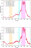 |
Fig. 9 Observed and modeled FUV spectra for two regions in PJ10. Upper panel: observed (red) and modeled (blue) FUV spectra for the region shown in the left panel of Fig. 7. The best fit is obtained with E0 = 54.23 keV and adjustment factors FCH4 = 2.0, FC2H2 = 0.3, FC2H6 = 0.4. This fit requires a CH4 enhancement and C2H2 depletion, suggesting a local atmospheric anomaly. Lower panel: observed (red) and modeled (blue) spectra for the region in the right panel of Fig. 7. The best fit is obtained with E0 = 15 keV and adjustment factors FCH4 = 1.0, FC2H2 = 1.0, and FC2H6 = 1.0. This configuration is consistent with the model atmosphere. |
Acknowledgements
V. Hue and B. Benmahi acknowledge support from the French government under the France 2030 investment plan, as part of the Initiative d’Excellence d’Aix-Marseille Université -- A*MIDEX AMX-22-CPJ-04. French authors acknowledge the support of CNES to the Juno and JUICE missions. This work was supported by the Fonds de la Recherche Scientifique --FNRS under Grant(s) No. T003524F. B. Bonfond is a Research Associate of the Fonds de la Recherche Scientifique - FNRS.
References
- Acton, C. H. 1996, Planet. Space Sci., 44, 65 [Google Scholar]
- Acton, C., Bachman, N., Semenov, B., & Wright, E. 2018, Planet. Space Sci., 150, 9 [Google Scholar]
- Ajello, J. M., Pryor, W., Esposito, L., et al. 2005, Icarus, 178, 327 [NASA ADS] [CrossRef] [Google Scholar]
- Bagenal, F., Adriani, A., Allegrini, F., et al. 2017, Space Sci. Rev., 213, 219 [Google Scholar]
- Benmahi, B. 2022, Theses, Université de Bordeaux [Google Scholar]
- Benmahi, B., Cavalié, T., Dobrijevic, M., et al. 2020, EPSC2020 [Google Scholar]
- Benmahi, B., Bonfond, B., Benne, B., et al. 2024a, A&A, 685, A26 [NASA ADS] [CrossRef] [EDP Sciences] [Google Scholar]
- Benmahi, B., Bonfond, B., Benne, B., et al. 2024b, A&A, 691, A91 [NASA ADS] [CrossRef] [EDP Sciences] [Google Scholar]
- Benne, B., Benmahi, B., Dobrijevic, M., et al. 2024, A&A, 686, A22 [NASA ADS] [CrossRef] [EDP Sciences] [Google Scholar]
- Bolton, S. J., Adriani, A., Adumitroaie, V., et al. 2017, Science, 356, 821 [Google Scholar]
- Bonfond, B., Gladstone, G., Grodent, D., et al. 2017, Geophys. Res. Lett., 44, 4463 [NASA ADS] [CrossRef] [Google Scholar]
- Bonfond, B., Yao, Z., Gladstone, G., et al. 2021, AGU Adv., 2, e2020AV000275 [CrossRef] [Google Scholar]
- Broadfoot, A. L., Belton, M. J. S., Takacs, P. Z., et al. 1979, Science, 204, 979 [NASA ADS] [CrossRef] [Google Scholar]
- Cavalié, T., Rezac, L., Moreno, R., et al. 2023, Nat. Astron., 7, 1048 [CrossRef] [Google Scholar]
- Clarke, J., Moos, H., Atreya, S., & Lane, A. 1980, ApJ, 241, L179 [NASA ADS] [CrossRef] [Google Scholar]
- Clarke, J. T., Ballester, G. E., Trauger, J., et al. 1996, Science, 274, 404 [Google Scholar]
- Clarke, J. T., Ballester, G., Trauger, J., et al. 1998, J. Geophys. Res.: Planets, 103, 20217 [NASA ADS] [CrossRef] [Google Scholar]
- Dols, V., Gérard, J.-C., Paresce, F., Prangé, R., & Vidal-Madjar, A. 1992, Geophys. Res. Lett., 19, 1803 [NASA ADS] [CrossRef] [Google Scholar]
- Foreman-Mackey, D., Hogg, D. W., Lang, D., & Goodman, J. 2013, PASP, 125, 306 [Google Scholar]
- Gérard, J.-C., Grodent, D., Dols, V., et al. 1994, Science, 266, 1675 [CrossRef] [Google Scholar]
- Giles, R. S., Hue, V., Greathouse, T. K., et al. 2023, J. Geophys. Res. (Planets), 128, e2022JE007610 [Google Scholar]
- Gladstone, G., & Skinner, T. 1989, NASA Special Publication Series, NASA-SP-494, 221, Document Section, 494 [Google Scholar]
- Gladstone, G., Versteeg, M., Greathouse, T., et al. 2017, Geophys. Res. Lett., 44, 7668 [NASA ADS] [CrossRef] [Google Scholar]
- Greathouse, T. K., Gladstone, G. R., Davis, M. W., et al. 2013, in UV, X-Ray, and Gamma-Ray Space Instrumentation for Astronomy XVIII, 8859, eds. O. H. Siegmund, International Society for Optics and Photonics (SPIE), 88590T [Google Scholar]
- Greathouse, T., Gladstone, R., Versteeg, M., et al. 2021, J. Geophys. Res.: Planets, 126, e2021JE006954 [CrossRef] [Google Scholar]
- Grodent, D. 2015, Space Sci. Rev., 187, 23 [CrossRef] [Google Scholar]
- Grodent, D., Gladstone, G., Gérard, J.-C., Dols, V., & Waite, J. 1997, Icarus, 128, 306 [NASA ADS] [CrossRef] [Google Scholar]
- Grodent, D., Waite Jr, J. H., & Gérard, J.-C. 2001, J. Geophys. Res.: Space Phys., 106, 12933 [Google Scholar]
- Gustin, J., Grodent, D., Gérard, J.-C., & Clarke, J. 2002, Icarus, 157, 91 [NASA ADS] [CrossRef] [Google Scholar]
- Gustin, J., Grodent, D., Ray, L., et al. 2016, Icarus, 268, 215 [NASA ADS] [CrossRef] [Google Scholar]
- Gérard, J.-C., Bonfond, B., Grodent, D., et al. 2014, J. Geophys. Res.: Space Phys., 119, 9072 [CrossRef] [Google Scholar]
- Gérard, J.-C., Bonfond, B., Mauk, B. H., et al. 2019, J. Geophys. Res.: Space Phys., 124, 8298 [Google Scholar]
- Harris, W., Clarke, J. T., McGrath, M. A., & Ballester, G. E. 1996, Icarus, 123, 350 [CrossRef] [Google Scholar]
- Hue, V., Kammer, J. A., Gladstone, G. R., et al. 2018, in Space Telescopes and Instrumentation 2018: Ultraviolet to Gamma Ray, eds. J.-W. A. Den Herder, K. Nakazawa, & S. Nikzad (Austin, United States: SPIE), 108 [Google Scholar]
- Hue, V., Giles, R. S., Gladstone, G. R., et al. 2021, J. Astron. Telesc. Instrum. Syst., 7, 044003 [Google Scholar]
- Hue, V., Cavalié, T., Sinclair, J. A., et al. 2024, Space Sci. Rev., 220, 85 [Google Scholar]
- Lilensten, J., Kofman, W., Wisemberg, J., Oran, E. S., & DeVore, C. R. 1989, Ann. Geophys., 7, 83 [NASA ADS] [Google Scholar]
- Liu, X., Ahmed, S. M., Multari, R. A., James, G. K., & Ajello, J. M. 1995, ApJ, 101, 375 [Google Scholar]
- Livengood, T. A. 1992, The Jovian Ultraviolet Aurora Observed with the IUE Spacecraft: Brightness and Color Distribution with Longitude (The Johns Hopkins University) [Google Scholar]
- Melin, H., Stallard, T. S., O’Donoghue, J., et al. 2025, J. Geophys. Res.: Space Phys., 130, e2025JA034261 [Google Scholar]
- O’Donoghue, J., Moore, L., Bhakyapaibul, T., et al. 2021, Nature, 596, 54 [CrossRef] [Google Scholar]
- Prangé, R., Rego, D., Pallier, L., et al. 1998, J. Geophys. Res.: Planets, 103, 20195 [CrossRef] [Google Scholar]
- Rodriguez-Ovalle, P., Fouchet, T., Guerlet, S., et al. 2024, J. Geophys. Res.: Planets, 129, e2024JE008299 [Google Scholar]
- Sinclair, J. A., Orton, G. S., Greathouse, T. K., et al. 2017, Icarus, 292, 182 [NASA ADS] [CrossRef] [Google Scholar]
- Sinclair, J. A., Orton, G. S., Greathouse, T. K., et al. 2018, Icarus, 300, 305 [Google Scholar]
- Sinclair, J. A., Orton, G. S., Fernandes, J., et al. 2019, Nat. Astron., 3, 607 [Google Scholar]
- Sinclair, J. A., Greathouse, T. K., Giles, R. S., et al. 2020, Planet. Sci. J., 1, 85 [NASA ADS] [CrossRef] [Google Scholar]
- Sinclair, J. A., West, R., Barbara, J. M., et al. 2023, Icarus, 406, 115740 [Google Scholar]
- Sinclair, J. A., Greathouse, T. K., Giles, R. S., et al. 2025, Planet. Sci. J., 6, 15 [Google Scholar]
- Tao, C., Kimura, T., Badman, S. V., et al. 2016, J. Geophys. Res.: Space Phys., 121, 4055 [Google Scholar]
- Trafton, L., Gerard, J.-C., Munhoven, G., & Waite Jr, J. 1994, ApJ, 421, 816 [NASA ADS] [CrossRef] [Google Scholar]
- Yung, Y. L., Gladstone, G. R., Chang, K. M., Ajello, J. M., & Srivastava, S. K. 1982, ApJ, 254, L65 [NASA ADS] [CrossRef] [Google Scholar]
Appendix A Justification for the redefinition of the CH4 absorption band
The standard CH4 CR uses the 125-130 nm interval as the absorption band (e.g., Gérard et al. 2019), due to its strong sensitivity to CH4. However, a detailed analysis of the Juno-UVS data revealed that this interval is frequently affected by detector calibration issues, notably due to distortions in the PHD. These artifacts primarily affect the wide slit measurements and manifest as underestimation of photon counts in high-brightness regions, leading to unreliable spectral intensities.
To mitigate these effects, several alternative intervals were tested and compared based on their correlation with the original CR and their intensity-to-noise ratio across multiple PJs (PJ1, PJ3, PJ6). Among these, the 135-140 nm band was found to offer the best compromise for the following reasons:
it lies within the CH4 absorption range;
it displays a intensity-to-noise ratio close to or higher than the original 125-130 nm interval in all tested regions (see Table A.1);
a comparative analysis of the PHD peak maps for PJ6 and PJ10 (Figs. A.1, A.2, A.3, A.4) shows that the 125-130 nm interval frequently exhibits PHD peaks below the nominal calibration threshold of 5, whereas the 135-140 nm interval remains within expected ranges. This confirms that the latter is significantly less affected by instrumental distortions.
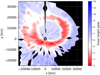 |
Fig. A.1 PHD peak map for the 125-130 nm interval during the whole duration of PJ6. Regions where the PHD peak falls below the nominal threshold of 5 are indicative of detector nonlinearity or calibration degradation. These pixels are considered unreliable for accurate spectral analysis. |
These conclusions were confirmed by comparing CR maps using different absorption intervals and by checking the PHD in regions where the correlation with the classical ratio broke down. In all cases, the 135-140 nm interval provided reliable and robust spectral behavior.
Thus, we adopted the following updated CH4 CR definition for this study:
 (A.1)
(A.1)
This redefinition ensures that the CR remains sensitive to CH4 absorption while minimizing instrumental biases due to nonlinearity and PHD degradation.
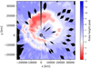 |
Fig. A.2 Same as Fig. A.1 but for PJ10. The PHD degradation in the 125-130 nm interval is also prominent here. |
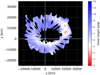 |
Fig. A.3 PHD peak map for the 135-140 nm interval during the whole duration of PJ6. Most regions exhibit PHD peaks above the calibration threshold, indicating reliable spectral response. |
INR comparison for different candidate absorption intervals in five representative auroral regions.
Appendix B Spectral flattening detection and correction method
The spectra gathered by Juno-UVS during PJ6 in the region of a dawn storm in the southern aurora are flattened and the CR maps that we construct from the spectral cube of this PJ cannot be used as a diagnostic for hydrocarbon absorption. To work around the high-flux nonlinearity effects that erode the spectral shape in high-brightness auroral regions, we develop a method to identify and correct the CR for pixels affected by this high-flux issue. Our approach relies on defining two narrow diagnostic bands within the unabsorbed portion of the H2 emission spectrum. These bands are selected based on both their spectral position and their sensitivity to instrumental degradation.
Band A: 157-158.5 nm, centered on the first of the two prominent peaks in the unabsorbed range of the H2 spectrum. This feature arises from strong Werner band emissions and is highly sensitive to spectral flattening in saturated observations.
Band B: 163-165 nm, located in a region of relatively smooth continuum, beyond the peak emission zone. This band serves as a stable normalization reference that is less susceptible to degradation of the PHD.
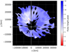 |
Fig. A.4 Same as Fig. A.3, but for PJ10. The 135-140 nm interval shows consistent detector performance across the auroral region. |
The motivation behind this selection is illustrated in Fig. B.1, which shows a representative H2 auroral spectrum obtained from PJ10 under nonsaturated conditions. Band A captures the height of a sharp spectral peak, making it a sensitive probe of any flattening due to gain compression. Band B, on the other hand, provides a reference baseline that is minimally affected by nonlinearities and changes in absorption.
Crucially, we also verified that the PHD in Band B remains systematically well-behaved, even in high-brightness regions where the unabsorbed 155-162 nm band is significantly degraded. This is demonstrated in Figs. B.2 and B.3, which show the PHD peak maps for band B during PJ6 and PJ10, respectively. In both cases, the PHD peak values remain above the nominal calibration threshold (typically set to 5), confirming that band B is less sensitive to detector high flux nonlinearity than the broader unabsorbed interval.
For comparison, the corresponding PHD peak maps for the 155-162 nm interval are shown in Figs. B.4 and B.5. These maps reveal extended regions with degraded PHDs (peak values below 5), especially within the brightest parts of the aurora. This contrast justifies the use of band B as a more reliable normalization anchor in our correction methodology.
We used TransPlanet simulations to compute the theoretical A/B intensity ratio under different auroral precipitation conditions. Specifically, six simulations were performed for electron energies of 1, 45, and 85 keV at both poles. The A/B ratios obtained are summarized in Table B.1. These values vary little across simulations, confirming that the 163-165 nm (band A) and 170-172 nm (band B) regions are minimally affected by hydrocarbon absorption. We therefore adopt the average ratio of 2.4639 as a reference baseline.
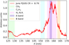 |
Fig. B.1 Example of an H2 auroral emission spectrum from PJ10, under nonsaturated conditions. The diagnostic bands A (violet) and B (orange) are highlighted. Band A captures the first emission peak, while band B provides a stable reference point. |
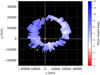 |
Fig. B.2 PHD peak values in band B (163-165 nm) during the whole duration of PJ6. The PHD remains within the nominal range across the entire auroral region, indicating that this spectral band is not significantly affected by detector nonlinearity during PJ6. |
Theoretical A/B intensity ratios from TransPlanet simulations.
Pixels exhibiting A/B ratios lower than 95% of the theoretical mean value are classified as degraded, provided that the B-band brightness exceeds 0.4 kR to limit the influence of photon noise. This dual criterion enables a robust detection of spectral distortions linked to detector nonlinearity in regions of high auroral brightness.
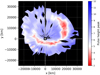 |
Fig. B.4 PHD peak values in the 155-162 nm band during the whole duration of PJ6. Regions with values below 5 (pink patches) are indicative of high flux and probable detector nonlinearity, particularly within the brightest parts of the aurora. |
For pixels flagged as spectrally degraded, the correction procedure relies on the assumption that the B band (163165 nm), located outside the main hydrocarbon absorption features, remains largely unaffected by detector nonlinearity for the studied perijoves. The observed intensity in this reference band is therefore considered reliable. By applying the theoretical A/B ratio, derived from TransPlanet simulations, we can reconstruct the expected intensity in Band A (155-162 nm), which is sensitive to detector nonlinearity.
This scaling allows us to estimate corrected CRs that more faithfully represent the true level of absorptions by CH4 and C2H2. Specifically, the corrected CH4 and C2H2 CRs are computed as
 (B.1)
(B.1)
 (B.2)
(B.2)
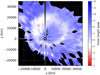 |
Fig. B.5 Same as Fig. B.4, but for PJ10. Spectral erosion is again apparent in the brightest auroral regions. |
This approach effectively compensates for the underestimation of flux in the unabsorbed band caused by detector nonlinearity, while preserving the integrity of the spectral information in unaffected regions.
Appendix C Uncorrected CR maps
The color ratio maps obtained using the standard color ratios for CH4 and C2H2 (Eqs. (2) and (3)) are displayed in Figs. C.1a and C.1b for PJ6 and in Figs. C.2a and C.2b for PJ10.
We identify unexpected absorption patterns in these maps. Indeed, several regions in both PJ6 and PJ10 exhibit apparent inconsistencies between CH4 and C2H2 absorptions. In each case, we identify two types of CR anomalies: zones where the CH4 CR is significantly elevated while the C2H2 CR remains low and conversely, zones with high C2 H2 CR but unexpectedly weak CH4 CR. These patterns pose a challenge to the expected vertical distribution of hydrocarbons, suggesting either instrumental effects or local variations in atmospheric composition. Comparing these maps to the ones obtained in Sect. 4 after applying the corrections presented in Sect. 3.3 is crucial to discriminate between these two hypotheses.
For PJ6, the CH4 CR map is largely unchanged compared to the corrected version, while the C2H2 CR map shows weak absorption in regions where pixels are affected by spectral flattening. After correction, these regions display stronger absorption, indicating that the anomalies were caused by instrumental effects.
On the other hand, for PJ10, both the spatial distributions of the CH4 CR and the C2 H2 CR remain largely unchanged between the corrected and uncorrected maps. This indicates that instrumental effects are not the main cause of anomalies and suggests the existence of real atmospheric heterogeneities rather than artifacts.
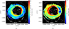 |
Fig. C.1 CR maps for PJ6 in the southern auroral region. Panels (a) and (b) show the uncorrected CH4 and C2H2 CR, respectively. A region centered near 70°S, 60°W (white arrow) exhibits strong CH4 absorption but weak C2H2 absorption, while an opposite pattern—low CH4 and enhanced C2H2 absorption—is observed around 75°S, 330°W (pink arrow). |
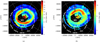 |
Fig. C.2 CR maps for PJ10 in the southern auroral region. Panels (a) and (b) show the uncorrected CH4 and C2H2 CR, respectively. A region centered near 85°S, 180°W (white arrow) exhibits strong CH4 absorption but weak C2H2 absorption, while an opposite pattern of low CH4 and enhanced C2H2 absorption is observed around 70°S, 30°W (pink arrow). |
All Tables
INR comparison for different candidate absorption intervals in five representative auroral regions.
All Figures
|
Fig. 1 Southern auroral H2 brightness maps integrated over the 155162 nm unabsorbed band for two perijoves: (a) PJ6 and (b) PJ10. |
| In the text | |
|
Fig. 2 Spectral diagnostics for hydrocarbon absorption and CR computation. Transparent green and cyan bands indicate the absorption spectral ranges used for CR calculations (125-130 nm for CH4, 150153 nm for C2H2), while the magenta band represents the nonabsorbed region assumed to be free of hydrocarbon absorption. The orange band is the new spectral range proposed for absorption of CH4 and the purple one is used to scale the color ratio in case of detector nonlinearity in the unabsorbed band (see Sect. 3.3). Upper panel: Simulated unabsorbed H2 spectrum from TransPlanet in dark blue. Lower panel: Corresponding optical depth for CH4, C2H2, and C2H6, showing the ranges used in CR calculations (from Benmahi et al. 2024a). |
| In the text | |
|
Fig. 3 Comparison of normalized PHDs in the 125-130 nm spectral band (blue) and the 135-140 nm spectral band (orange) during PJ10 for the region between 70°S and 73°S and between 30°W and 60°W. The orange histogram (135-140 nm) shows a well-calibrated distribution with a peak above 5. The blue histogram (125-130 nm) shows a PHD with a degraded shape and a peak below 5, indicating significant signal loss. |
| In the text | |
|
Fig. 4 Comparison between a spectrum affected by instrumental flattening (red) and an unaffected spectrum (blue), both extracted from the same auroral region during PJ6. The affected spectrum, observed with the wide slit in a very bright area, exhibits a flattened shape with missing emission features particularly in the unabsorbed band. In contrast, the narrow-slit spectrum in the same region clearly shows the characteristic double-peaked H2 continuum around 160 nm. |
| In the text | |
|
Fig. 5 CR maps for PJ6 in the southern auroral region after applying the corrections presented in Sect. 3.3. Right panel: CR map for CH4. Left panel: CR map for C2H2. The corrected regions are highlighted in Fig. 6. |
| In the text | |
|
Fig. 6 Mask map showing the correction applied to CR maps of PJ6. The purple pixels have not been corrected and the green ones have been replaced by the corrected CRs (Eqs. (6) and (7)). |
| In the text | |
|
Fig. 7 CR maps for PJ10 in the southern auroral region after applying the corrections presented in Sect. 3.3. Right panel: CR map for CH4. Left panel: CR map for C2H2 The corrected regions are highlighted in Fig. 8. A region centered near 85°S, 180°W exhibits strong CH4 absorption but weak C2H2 absorption, while an opposite pattern (low CH4 and enhanced C2H2 absorption) is observed around 70°S, 30°W. Dashed white polygons outline regions with contrasting CR behaviors. |
| In the text | |
|
Fig. 8 Mask map showing the correction applied to CR maps of PJ10. The purple pixels have not been corrected, while the green ones have been replaced by the corrected CRs (Eqs. (6) and (7)). |
| In the text | |
|
Fig. 9 Observed and modeled FUV spectra for two regions in PJ10. Upper panel: observed (red) and modeled (blue) FUV spectra for the region shown in the left panel of Fig. 7. The best fit is obtained with E0 = 54.23 keV and adjustment factors FCH4 = 2.0, FC2H2 = 0.3, FC2H6 = 0.4. This fit requires a CH4 enhancement and C2H2 depletion, suggesting a local atmospheric anomaly. Lower panel: observed (red) and modeled (blue) spectra for the region in the right panel of Fig. 7. The best fit is obtained with E0 = 15 keV and adjustment factors FCH4 = 1.0, FC2H2 = 1.0, and FC2H6 = 1.0. This configuration is consistent with the model atmosphere. |
| In the text | |
|
Fig. A.1 PHD peak map for the 125-130 nm interval during the whole duration of PJ6. Regions where the PHD peak falls below the nominal threshold of 5 are indicative of detector nonlinearity or calibration degradation. These pixels are considered unreliable for accurate spectral analysis. |
| In the text | |
|
Fig. A.2 Same as Fig. A.1 but for PJ10. The PHD degradation in the 125-130 nm interval is also prominent here. |
| In the text | |
|
Fig. A.3 PHD peak map for the 135-140 nm interval during the whole duration of PJ6. Most regions exhibit PHD peaks above the calibration threshold, indicating reliable spectral response. |
| In the text | |
|
Fig. A.4 Same as Fig. A.3, but for PJ10. The 135-140 nm interval shows consistent detector performance across the auroral region. |
| In the text | |
|
Fig. B.1 Example of an H2 auroral emission spectrum from PJ10, under nonsaturated conditions. The diagnostic bands A (violet) and B (orange) are highlighted. Band A captures the first emission peak, while band B provides a stable reference point. |
| In the text | |
|
Fig. B.2 PHD peak values in band B (163-165 nm) during the whole duration of PJ6. The PHD remains within the nominal range across the entire auroral region, indicating that this spectral band is not significantly affected by detector nonlinearity during PJ6. |
| In the text | |
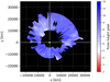 |
Fig. B.3 Same as Fig. B.2 but for PJ10. Again, band B exhibits consistently calibrated PHD values. |
| In the text | |
|
Fig. B.4 PHD peak values in the 155-162 nm band during the whole duration of PJ6. Regions with values below 5 (pink patches) are indicative of high flux and probable detector nonlinearity, particularly within the brightest parts of the aurora. |
| In the text | |
|
Fig. B.5 Same as Fig. B.4, but for PJ10. Spectral erosion is again apparent in the brightest auroral regions. |
| In the text | |
|
Fig. C.1 CR maps for PJ6 in the southern auroral region. Panels (a) and (b) show the uncorrected CH4 and C2H2 CR, respectively. A region centered near 70°S, 60°W (white arrow) exhibits strong CH4 absorption but weak C2H2 absorption, while an opposite pattern—low CH4 and enhanced C2H2 absorption—is observed around 75°S, 330°W (pink arrow). |
| In the text | |
|
Fig. C.2 CR maps for PJ10 in the southern auroral region. Panels (a) and (b) show the uncorrected CH4 and C2H2 CR, respectively. A region centered near 85°S, 180°W (white arrow) exhibits strong CH4 absorption but weak C2H2 absorption, while an opposite pattern of low CH4 and enhanced C2H2 absorption is observed around 70°S, 30°W (pink arrow). |
| In the text | |
Current usage metrics show cumulative count of Article Views (full-text article views including HTML views, PDF and ePub downloads, according to the available data) and Abstracts Views on Vision4Press platform.
Data correspond to usage on the plateform after 2015. The current usage metrics is available 48-96 hours after online publication and is updated daily on week days.
Initial download of the metrics may take a while.