| Issue |
A&A
Volume 707, March 2026
|
|
|---|---|---|
| Article Number | A241 | |
| Number of page(s) | 14 | |
| Section | Galactic structure, stellar clusters and populations | |
| DOI | https://doi.org/10.1051/0004-6361/202557046 | |
| Published online | 17 March 2026 | |
A closer look at the young stellar group around Sh 2-295
Universidade de São Paulo, Instituto de Astronomia, Geofísica e Ciências Atmosféricas,
Rua do Matão 1226,
São Paulo,
SP,
05508-090,
Brazil
★ Corresponding author: This email address is being protected from spambots. You need JavaScript enabled to view it.
Received:
30
August
2025
Accepted:
23
December
2025
Abstract
Context. Star formation is governed by multiple physical processes, making it inherently complicated. One excellent example is the Canis Major OB1/R1 association, whose complex history of star formation is related to different episodes. Three supernova (SN) events potentially altered the environment and impacted star formation and stellar evolution.
Aims. Prior investigations revealed two stellar groups of different ages associated with GU CMa and Z CMa. This work focusses on identifying the low-mass young stellar population near FZ CMa, located between these two groups and spatially related to the H II region Sh 2-295. Our main goal is to verify whether this group is age-mixed and characterise its physical properties.
Methods. We analysed multi-object spectroscopic data acquired with Gemini/GMOS to search for typical features of T Tauri stars (TTs) and to determine their spectral types. Lithium absorption line (λ6708 Å) was used as a youth indicator, while Hα emission was investigated to probe accretion activity. We also derived ages based on optical photometry from Gaia DR3 and compared the projected spatial distribution to diffuse infrared emission.
Results. We identified 29 TTs, including six new members of the association and three classical TTs. The equivalent width of the Li I absorption line suggests an age of 8.1−3.8+2.1 Myr, while optical photometric data indicate stellar ages ranging from ~1 to 14 Myr. Younger stars are concentrated around Sh 2-295, whereas the older ones are more widely dispersed.
Conclusions. We increased the number of known TTs related to the CMa association. Our results support a scenario of multiple star formation episodes, including a younger group that may have been triggered by the expansion of Sh 2-295. The influence of SN events appears limited in this context.
Key words: stars: formation / stars: fundamental parameters / stars: low-mass / stars: pre-main sequence / stars: variables: T Tauri, Herbig Ae/Be
© The Authors 2026
 Open Access article, published by EDP Sciences, under the terms of the Creative Commons Attribution License (https://creativecommons.org/licenses/by/4.0), which permits unrestricted use, distribution, and reproduction in any medium, provided the original work is properly cited.
This article is published in open access under the Subscribe to Open model. This email address is being protected from spambots. You need JavaScript enabled to view it. to support open access publication.
1 Introduction
The Canis Major OB1/R1 association is one of the most intriguing star-forming regions in our Galaxy. It is located approximately 1 kpc away (Gregorio-Hetem 2008; Santos-Silva et al. 2021; Dong et al. 2024) and spans a large area (over 80 sq. deg. Fernandes et al. 2019). The region encompasses several reflection and emission nebulae including the H II regions Sh 2-292, Sh 2-293, Sh 2-295, Sh 2-296, and Sh 2-297 (Sharpless 1959). These nebulae are mainly located in the central part of the association coinciding with the main molecular clouds (222 deg < l < 227 deg, −3 deg < b < 0 deg). This central region (hereafter CMa region), contains stellar groups spanning a wide age range (~1.5–18 Myr – Fernandes et al. 2015; Santos-Silva et al. 2021). Despite extensive studies, the star formation history of CMa remains unclear.
Sh 2-296 is the most notable nebula in CMa. It has an arc-like shape and, together with the absence of luminous stellar objects and the presence of the runaway star HD 54662, led Herbst & Assousa (1977) to propose that a supernova (SN) triggered star formation in CMa. Alternatively, Comeron et al. (1998) suggested that the star formation occurred in the pre-existing clouds, and that the stars were subsequently compressed and accelerated by the SN explosion.
More recently, Fernandes et al. (2019) proposed that Sh 2-296 is part of a larger, roughly ellipsoidal structure named CMa-shell, with a diameter of about 60 pc. They also identified three runaway stars likely ejected from a similar location within the shell. These features were interpreted as consequences of three successive SN explosions that happened ~6 Myr, 2 Myr, and 1 Myr ago. However, the formation of the older stellar population could not be linked to these events. Therefore, the authors suggested that the SNe had only a minimal role in triggering star formation.
In order to reconstruct a three-dimensional morphology and kinematics of gas distribution compared with the stellar population of the CMa region, Dong et al. (2024) used 12CO, 13CO, and C18O (1–0) along with astrometric data from Gaia Data Release 3 (DR3, Gaia Collaboration 2023). Their results support the presence of a slowly expanding shell (1.6 ± 0.7 km s−1), formed by at least two SN events, in agreement with the findings of Fernandes et al. (2019).
A 5 square degree X-ray survey conducted using the ROSAT satellite in the western part of the shell revealed the existence of two groups of differing ages, named after the nearest bright stars: GU CMa and Z CMa (Gregorio-Hetem et al. 2009). The GU CMa group lies further from the main molecular cloud, in contrast to the Z CMa group. Santos-Silva et al. (2018) revisited part of this area with more sensitive XMM-Newton observations. They found that most stars near Z CMa are younger than 5 Myr, whereas the bulk of the GU CMa population is older than 10 Myr. These results support a two-epoch formation scenario: the first episode occurred ~10 Myr ago across the entire region, and a second, more recent episode (<5 Myr) took place in areas where there was still molecular gas.
Fernandes et al. (2015) identified 58 objects – 41 confirmed T Tauri stars (TTs) and 17 young star candidates – close to Z CMa using X-ray detections and optical spectroscopy. Among the TTs, 17% are classical TTs (CTTs), while 83% are weak-lined TTs (WTTs). Based on infrared (IR) excess, they also estimated a low fraction (~25%) of disc-bearing stars compared to other young groups with similar ages (1–2 Myr). This fraction may be related to early dissipation due to shock waves from a SN.
Our main goal is to improve the census of the low-mass young stars towards the region between Z CMa and GU CMa (the ‘inter-cluster region’) that includes FZ CMa, a B2 IVn star (Shevchenko et al. 1999) associated with the H II region Sh 2-295. The stellar population in this area is likely to be mixed in age. Our goal is twofold: (i) to characterise this population to assess whether it is indeed mixed, and (ii) to better understand the possible effects of SNe on star formation in the region. This study aims to add another piece to the CMa puzzle. The paper is organised as follows. Section 2 describes Gemini spectroscopic data acquisition and reduction. Section 3 details the spectral analysis. In Sect. 4, we discuss the ages derived from photometry based on the colour-magnitude diagram (CMD), and compare them with dust distribution (mid-infrared emission). Finally, the main findings and conclusions are summarised in Sect. 5.
2 Observations and data reduction
Optical spectroscopy was performed in March 2017 using the 8 m Gemini South telescope with the Gemini Multi-Object Spectrograph (GMOS). The observations were part of programmes GS-2013A-Q-68 (pre-imaging and mask preparation) and GS-2017A-Q-23 (spectra acquisition).
The instrumental set-up consisted of the R831 grating centred at 6700 Å and 6750 Å, with a 1″ slit width and 2 × 2 pixel binning. Two central wavelengths were chosen to prevent spectral gaps between the detectors. According to Gemini grating specifications1, this configuration yields a resolving power of about 2200 at the blaze wavelength (λ7570 Å). Each spectrum covers different wavelength ranges due to the mask configuration and the resulting variation in incidence angle. However, the whole set of spectra covers, at least, wavelengths from 5995 Å to 7412 Å.
A total of 137 stars were observed across four distinct fields, each with a field of view (FoV) of 5.5′ × 5.5′. The fields were selected to encompass the majority of X-ray sources previously identified in the inter-cluster region. Approximately 18% of the sample have X-ray counterparts compatible with YSOs (Santos-Silva et al. 2018). The additional candidates were included to complete the observable field. Each target was observed with an exposure time of 1030 s. Figure 1 shows the GMOS fields and all observed stars in comparison with X-ray sources. A summary of the characteristics of each field is presented in Table 1.
GMOS spectroscopic data were reduced using the GEMINI/IRAF2 package. We followed a standard procedure, which is described in the GMOS data reduction cookbook3 (Merino et al. 2022) and is similar to that adopted by Stanghellini et al. (2014). The procedure consists of eight main steps: bias subtraction; flat-fielding; wavelength calibration; spectra cutting; cosmic ray and bad pixel rejection; spectra extraction; sky subtraction; and flux calibration.
In addition to the standard calibration process, a procedure was necessary to refine the astrometry. A crossmatch between GMOS, Gaia DR3 (Gaia Collaboration 2023), and the Two Micron All Sky Survey (2MASS – Skrutskie et al. 2006) was performed by selecting the nearest source within a maximum separation of 1″. We found quasi-systematic positional offsets relative to the candidate counterparts that varied (0.5–1.3″) across the fields. In order to correct these effects of telescope pointing, a constant shift was added to the equatorial co-ordinates of each source within a given field (ΔRA, ΔDec given in Table 1).
Characteristics of the observed GMOS fields.
3 Spectral analysis
After reducing and calibrating the GMOS spectra, we examined key spectral features typically used to identify low-mass pre-main-sequence (PMS) stars. These features allowed us to characterise our sample in terms of accretion activity and stellar youth. In this section, we describe the methodology adopted to analyse the spectroscopic data.
3.1 Identification of TTs
To identify TTs in our sample, we followed the methodology of Fernandes et al. (2015). The procedure consists of searching for typical spectroscopic features, such as Hα emission and absorption in the Li I line (λ6708 Å). Most of these features were identified in the individual spectra and in the combined spectrum, except in regions affected by artefacts such as cosmic rays.
Among the 137 spectra analysed, we found 24 objects showing both Hα emission and Li I absorption and 5 objects showing only Li I absorption. These 29 objects were classified as TTs. Table 2 presents the equivalent widths, W(Hα) and W(Li), of these objects, listed by their 2MASS counterpart identification. The spectrum of the object 2MASS J07033726-1131146 is presented in Fig. 2 as an example of TTs with Hα emission and Li I absorption. The spectra of the remaining 28 objects are presented in Appendix A. We also found seven objects with Hα emission but no lithium absorption. Since they are faint stars (G > 16 mag), these may be main-sequence dwarfs with Hα emission (dMe). A list of these objects is provided in Appendix B, but they will not be further discussed in this paper.
The signal-to-noise ratio (S/N) of all spectra centred at 6700 Å is reported in Table 2 as an indicator of spectral quality. These values were computed using the specutils Python package and represent mean values measured over the 6450–6550 Å and 6600–6700 Å intervals. The S/N for spectra centred at 6750 Å are similar.
To measure the equivalent width (W), we followed a procedure similar to that proposed by Martin et al. (1998) and Alcalá et al. (2002). We performed repeated measurements while varying the continuum level. The mean of these measurements was adopted as our W estimate.
Typical relative uncertainties (σW/W) range from 1% to 10%, corresponding to σW ~0.02 Å for Li and σW ~ 0.1 Å for Hα. These mainly arise from uncertainties in the continuum choice and line profile. Given the medium spectral resolution, unresolved blending with nearby lines – such as Fe I λ6710 Å – may have also affected the measurements.
Among the 29 TTs identified in this work, six are new discoveries, while 23 were previously reported in the literature as possible PMS stars. Table 2 summarises the available information indicating sources that are X-ray emitters (Santos-Silva et al. 2018); membership probability based on proper motions from Gaia DR2 (Gregorio-Hetem et al. 2021); IR classification suggesting Class II or Class III objects (Fischer et al. 2016; Santos-Silva et al. 2018); and Hα emission (Pettersson & Reipurth 2019).
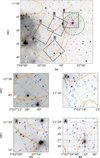 |
Fig. 1 Top panel: optical (Digitized Sky Survey – DSS2, F+R) image of the region studied in this work. The black squares indicate the GMOS 1–4 fields of Table 1. The dashed green circle shows the Sh 2-295 H II region (Sharpless 1959). Bottom panel: GMOS R pre-images used to prepare GMOS masks. To facilitate the identification of the co-ordinate system orientation in each image, the grid lines corresponding to RA and Dec are plotted in grey as dashed and solid lines, respectively. The position of the slits are shown by open blue squares. In both panels, orange lines represent AV = 1 and AV = 3 mag contours (Cambrésy, priv. commun.) and open magenta circles indicate X-ray sources (Santos-Silva et al. 2018). Note that not all X-ray sources were covered by the GMOS observations. |
List of TTs identified and parameters derived in this work.
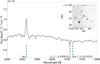 |
Fig. 2 Example of a GMOS spectrum highlighting Hα emission, and Li I (λ6708 Å) and Ca I (λ6718 Å) absorption features. The top right panel shows the angular position of a TTs (green circle) compared to X-ray sources (black circles – Santos-Silva et al. 2018), confirming it as an X-ray counterpart. |
3.2 Spectral classification
Spectral types were estimated using two different methods: (i) numerical and visual comparison with spectra of known spectral types; and (ii) spectral indices sensitive to spectral type. Both methods are described as follows.
In the first method, we compared the GMOS spectra with two libraries of young star templates. To perform it consistently, all spectra were degraded to the lower resolution of each pair, and comparisons were made using the template_match function from the specutils Python package (Earl et al. 2025) to calculate a goodness of fit expressed by
![Mathematical equation: $\[G=\sum_\lambda\left[\frac{C_{A_V}(\lambda)-\alpha T(\lambda)}{\sigma_C(\lambda)}\right]^2.\]$](/articles/aa/full_html/2026/03/aa57046-25/aa57046-25-eq2.png) (1)
(1)
CAV (λ) is the observed GMOS spectrum including the effects of visual extinction (AV), σC(λ) are the associated uncertainties, and T(λ) is the template spectrum. α is the flux-scaling factor determined by the function _normalize_for_template_matching from specutils as well. This method was adapted from Manjavacas et al. (2020) and Cushing et al. (2008).
Two distinct libraries of spectral types were used separately:
A sub-sample from Luhman et al. (2018, L18) with 14 spectra (from stars with ages ~11 Myr) covering K6–M7 types, with a typical uncertainty of 0.25 spectral types. The resolution varies between 3 and 4 Å and the extinction is relatively low (AV ≲ 1.0 mag). For spectral types earlier than K2, we included spectra of dwarfs (or subgiants when dwarfs were not available) from STELIB (Le Borgne et al. 2003). These objects have different surface gravities when compared to their younger counterparts and may exhibit significant extinction. Although this library is not specific to young stars, no systematic effect is introduced because our method for this range of earlier spectral types is based on the continuum shape, which is not affected by differences in surface gravity.
A grid of 28 spectra of photospheric templates from Claes et al. (2024, C24). This grid is dereddened and covers G5 to M9.5 spectral types, although it is incomplete, especially for G-type stars.
For each object the best-fitting spectral type and AV were estimated simultaneously by minimising G. To do this, the ![Mathematical equation: $\[A_{V}^{s t}\]$](/articles/aa/full_html/2026/03/aa57046-25/aa57046-25-eq3.png) that best fits each spectral type was first determined by varying it from 0 to 5.75 mag using 0.25 mag steps. This range was adopted according to the limits indicated by dust extinction maps available for the CMa region. Spectra were dereddened using the dust_extinction Python package and the extinction curve from Gordon et al. (2023). We adopted RV = AV/E(B − V) = 3.1 as a typical Galactic value, although larger values are possible in dense environments (e.g. Fitzpatrick 1999). The second step was to compare each pair (by spectral type,
that best fits each spectral type was first determined by varying it from 0 to 5.75 mag using 0.25 mag steps. This range was adopted according to the limits indicated by dust extinction maps available for the CMa region. Spectra were dereddened using the dust_extinction Python package and the extinction curve from Gordon et al. (2023). We adopted RV = AV/E(B − V) = 3.1 as a typical Galactic value, although larger values are possible in dense environments (e.g. Fitzpatrick 1999). The second step was to compare each pair (by spectral type, ![Mathematical equation: $\[A_{V}^{s t}\]$](/articles/aa/full_html/2026/03/aa57046-25/aa57046-25-eq4.png) ), in order to find the one that best reproduces the observed data. Visual inspection was used to confirm or refine the classification. An example of the spectral type and AV determined by this method is presented in Fig. 3. Comparisons between our AV estimates and other methodologies are presented in Appendix C.
), in order to find the one that best reproduces the observed data. Visual inspection was used to confirm or refine the classification. An example of the spectral type and AV determined by this method is presented in Fig. 3. Comparisons between our AV estimates and other methodologies are presented in Appendix C.
The wavelength intervals used in spectral comparison were selected to account for both temperature-sensitive features and/or the continuum. We considered the regions listed in C24 and those required to calculate the spectral indices from Herczeg & Hillenbrand (2014, HH14) – some of these regions were also used in the second method. Table 3 lists the ranges and corresponding spectral features. Regions affected by telluric bands, strong emission lines (e.g. Hα), or spectral defects were excluded.
In the second method, we computed three spectral indices: TiO 6800 (ideal for K5–M0.5) and TiO 7140 (for M0–M4.5) from HH 14, and the TiO index from Jeffries et al. (2007, J07 – designed to K5–M0 stars). These indices provide a method of spectral typing by comparing the flux of different spectral narrow ranges that are sensitive to temperature to continuum ranges. As was mentioned by HH 14, the conversion between spectral indices to spectral types is sensitive to S/N and to the relative flux calibration. Gravity and metallicity differences can also affect the results.
Typical discrepancies between the two methods were within one spectral subtype (see Appendix D), which we adopted as the uncertainty. However, the uncertainty could be larger for earlier type stars, where the grids are limited, molecular bands tend to disappear, and the spectral indices used are less discriminating. Some stars also showed degenerate combinations of AV and spectral type, introducing larger uncertainties. The results were cross-validated by using photometric data to construct a CMD (see Sect. 4.1). The adopted values are shown in Table 2.
Effective temperatures (Teff) were assigned as a function of spectral type by adopting the relationship obtained by Pecaut & Mamajek (2013) for stars between 5 and 30 Myr. The mean temperature step between adjacent spectral types is ~120 K, adopted as the uncertainty for one subtype. For stars with larger spectral type uncertainty, the maximum relative error adopted is about ~9%.
It is also important to mention that here we adopt a simple single-temperature model for the GMOS spectra. This may introduce biases in the derived stellar parameters of the spotted PMS, as has been shown by Pérez Paolino et al. (2025).
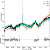 |
Fig. 3 Example of spectral typing via spectral comparison. The GMOS spectrum, normalised by the flux at 7050 Å, is shown in black in the regions used to calculated G and in grey elsewhere. The pair AV = 0.75 mag, and M2-type stellar spectrum (green line) represents the best fit to the object. For comparison, spectra of M-1 and M-3 type stars are shown in blue and orange, respectively. The bottom panel shows the residuals of the comparison between the GMOS object and the M2-type stellar spectrum. |
Spectral regions used for spectral classification.
3.3 Classification of CTTs and WTTs
In CTT, spectral features associated with the accretion process include an emission line spectrum, the presence of forbidden lines, and photospheric continuum excess (e.g. Barrado y Navascués & Martín 2003). In particular, Hα emission tends to be broad and may present asymmetries. The spectrum of WTTs can have Hα in emission as well; however, they show smaller equivalent widths when compared to CTTs (Barrado y Navascués & Martín 2003). In this case, the emission is associated with chromospheric activity (e.g. Fernandes et al. 2015).
Several criteria were proposed to distinguish between CTTs and WTTs in the literature. Here we adopt two criteria based on the equivalent width of the Hα emission line: the saturation criterion proposed by Barrado y Navascués & Martín (2003) and the empirical criterion to determine non-veiled TTs from White & Basri (2003).
Stars with W(Hα) above the thresholds proposed by these authors are classified as CTTs; otherwise, they are considered WTTs. Figure 4 shows the W(Hα) for the 24 stars with Hα emission compared to both these thresholds. For clarity, uncertainties in spectral type are not shown, while uncertainties in W(Hα) are typically of the same order as the symbol size.
Only three stars meet both criteria and are classified as CTTs. One additional star fulfils only the Barrado y Navascués & Martín (2003) criterion. We consider it as a WTT candidate (WTT?). Considering the adopted uncertainties, the object 07024945-1125470 can also fulfil the Barrado y Navascués & Martín (2003) criterion. Therefore, it is also considered a WTT candidate. Thus, 10% of the sample is confirmed as CTTs (excluding WTTs).
For comparison, Fig. 4 also shows the classification adopted by Fernandes et al. (2015) in a study of the region associated with the Z CMa system (grey symbols). These authors found a CTT fraction of 17% in a region where the gas is more concentrated than the region associated with FZ CMa. Indeed, these fractions should not be considered as representative of the whole region, since a small sample was analysed.
3.4 Lithium
One valuable indicator of youth in the stellar spectrum is the presence of lithium (e.g. Fernandes et al. 2015; Pecaut & Mamajek 2016; Jeffries et al. 2007). At very young ages, while the central temperatures are lower than 2.5 × 10⁶ K, lithium is preserved. As the star evolves to the main sequence, the central temperature increases, convective mixing transports Li to the inner regions, and the element is depleted via proton capture (Ushomirsky et al. 1998). Thus, in low-mass stars, a high photospheric lithium abundance is observed only in very young stars (Pecaut & Mamajek 2016). Therefore, this is a distance-independent indicator of youth (Soderblom et al. 2014). When various clusters in different evolutionary stages are compared, a trend of decreasing lithium abundance with age is clearly seen, as, for instance, in Pecaut & Mamajek (2016) and Jeffries et al. (2023).
In Fig. 5, we show W(Li) as a function of effective temperature for the FZ CMa and Z CMa groups. A scatter trend is similar for both, which may reflect an age dispersion, different rotation rates, or accretion history, as was pointed out by Fernandes et al. (2015).
Polynomial fits from Pecaut & Mamajek (2016, and references therein) for Sco-Cen (~10–16 Myr), IC 2602 (~45 Myr), and Pleiades (~125 Myr) are overplotted for comparison. Our sample lies between Sco-Cen and Z CMa in this diagram.
We also used the code ‘Estimating AGes from Lithium Equivalent widthS’ (EAGLES) v2 (Jeffries et al. 2023; Weaver et al. 2024) to infer the most probable age of the FZ CMa group based on W(Li). The code employs an artificial neural network model of the relationship between Teff, age, and W(Li) also including its intrinsic dispersion. The EAGLES v2 code estimates ![Mathematical equation: $\[8.1_{-3.8}^{+2.1}\]$](/articles/aa/full_html/2026/03/aa57046-25/aa57046-25-eq5.png) Myr for this group, which is in accordance with the age expected, as was mentioned before. However, precision is lower for clusters with log (age/yr) ≲ 7.1 when compared to slightly older clusters (Weaver et al. 2024).
Myr for this group, which is in accordance with the age expected, as was mentioned before. However, precision is lower for clusters with log (age/yr) ≲ 7.1 when compared to slightly older clusters (Weaver et al. 2024).
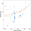 |
Fig. 4 Thresholds defining the CTT classification following White & Basri green dashed line (2003) and Barrado y Navascués & Martín orange dash-dotted line (2003). Blue symbols represent our sample; grey symbols are data from Fernandes et al. (2015). These criteria were used to classify the CTTs (indicated by circles), WTTs (triangles), and possible WTTs (crosses). |
4 Contrasting ages and angular distribution
After identifying TTs based on spectroscopic diagnostics, we characterised our sample in terms of age. This allowed us to assess whether the population is indeed mixed, as was suggested in previous works. To do that, we used optical photometric data from Gaia DR3 (Gaia Collaboration 2023) and compared it to theoretical models in CMD. This dataset, independent of the GMOS spectra, also served to verify the adopted spectral types. In Sect. 4.2, we explore the angular distribution of the sources to identify potential correlations between spatial location and stellar ages, which could shed light on the formation history of the region.
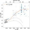 |
Fig. 5 W(Li) from the 6708 Å line vs Teff and spectral type. Symbols and colours are the same as in Fig. 4. Grey lines are polynomial fits for observed data in other young clusters: Sco-Cen (10–16 Myr), IC2602 (45 Myr), and Pleiades (125 Myr) – see Pecaut & Mamajek (2016) and references therein. The orange line represents the expected curve for a population of |
![Mathematical equation: $\[8.1_{-3.8}^{+2.1}\]$](/articles/aa/full_html/2026/03/aa57046-25/aa57046-25-eq6.png)
4.1 CMD ages
Determining an accurate age estimation for each star could be very challenging, but it is important to disentangle the history of star formation of different clusters. To constrain the age range of the TTs in our sample, we compared Gaia DR3 photometric data to PAdova and tRieste Stellar Evolutionary Code (PARSEC) isochrones (release v1.2S + COLIBRI S_37 + S_35 + PR16 – see Bressan et al. 2012; Chen et al. 2014, 2015; Tang et al. 2014; Marigo et al. 2017; Pastorelli et al. 2019, 2020, and references therein). Based on previous age estimates for this region, we adopted PARSEC isochrones ranging from 1 to 20 Myr equally spaced by 0.25 Myr.
Among 29 TTs, we found matching photometric data for 23 objects in a 1″ maximum separation. We only considered sources with RUWE4 ≤ 1.4, indicating good astrometric quality. This criterion was adopted to ensure that reliable counterparts were identified, from which we adopted the photometric data. The remaining six stars did not meet these criteria. To convert apparent magnitudes into absolute magnitudes, we relied on literature values. Two previously reported clusters lie along the same line of sight of the inter-cluster region: VdBerg 92 (e.g. He et al. 2022) and CMa 06 (Santos-Silva et al. 2021). Santos-Silva et al. (2021) argue that VdBerg 92 is only part of the CMa 06 group, which was suggested by the spatial distribution and number of members. The astrometric distance of CMa 06 is ![Mathematical equation: $\[1147_{-133}^{+77}\]$](/articles/aa/full_html/2026/03/aa57046-25/aa57046-25-eq7.png) pc. The inter-cluster region is also located in the direction of sub-region B studied by Dong et al. (2024) – d = (1087 ± 19) pc. Therefore, we adopted a mean distance of d = 1117 pc.
pc. The inter-cluster region is also located in the direction of sub-region B studied by Dong et al. (2024) – d = (1087 ± 19) pc. Therefore, we adopted a mean distance of d = 1117 pc.
Extinction corrections were applied to the CMD using the relations AG/AV = 0.83627, ABP/AV = 1.08337, and ARP/AV = 0.63439 (Cardelli et al. 1989; O’Donnell 1994), respectively, corresponding to the effective wavelengths 6390.21 Å, 5182.58 Å, and 7825.08 Å of the Gaia filter passbands. These relations are consistent with the extinction curve from Gordon et al. (2023). The AV values were adopted from the spectral fitting (Sect. 3.2).
As no degeneracies are present in the CMD region that encompasses our data, we estimated age ranges by finding the closest isochrones to each data point. They were determined by calculating the minimum distance between each source and each isochrone in the colour-magnitude space following the equation
![Mathematical equation: $\[d_{min }=\min _i \sqrt{\left(x-x_i^{i s o c}\right)^2+\left(y-y_i^{i s o c}\right)^2},\]$](/articles/aa/full_html/2026/03/aa57046-25/aa57046-25-eq8.png) (2)
(2)
in which x represents the colour (GBP − GRP)0, y is the absolute magnitude in the Gaia G band, and the subscript i denotes each individual point along the isochrone curve (which has been interpolated to improve accuracy).
The estimated age ranges are reported in Table 2. We caution that these results depend on multiple uncertainties regarding photometry, extinction estimates, unresolved multiplicity, distance, and model assumptions. The bottom panel of Fig. 6 shows the extinction-corrected CMD. Photometric uncertainties are typically symbol size and tend to be higher for faint sources. An illustration of the expected error bar due to large photometric uncertainties is shown in Fig. 6 for the faintest source of the sample.
The top panel of Figure 6 shows a histogram of the ages estimated for the FZ CMa group. The distribution of ages in our sample indicates that 13 stars (57%) are younger than 5 Myr, 7 (30%) are 5–10 Myr old, and 3 (13%) are 10–14 Myr old. It is worth noting that these few older objects are among the faintest, for which the age estimates are less reliable. These results are consistent with what was estimated via lithium depletion, and to what was found for the VdBerg 92 cluster (~5.6 Myr – He et al. 2022). It is also consistent with the fact that CMa 06 has a large spread in CMD (Santos-Silva et al. 2021), with most of the stars coinciding with isochrones from 1 Myr to 6 Myr.
4.2 Angular distribution
Figure 7 shows the projected spatial distribution of the TTs found in this work overlaid on a two-colour composite with mid-infrared widefield infrared survey explorer (WISE – Wright et al. 2010) W3 (12 μm) and W4 (22 μm) bands. The Sh 2-295 H II region is clearly seen as an arc-like structure. According to Anderson et al. (2014, and references therein), polycyclic aromatic hydrocarbon (PAH) molecules are the ones that mainly contribute to emission in the W3 band in H II regions, while the W4 band traces small dust grains that were stochastically heated.
A spatial correlation is apparent between the position of many TTs and the regions of enhanced IR emission, particularly around Sh 2-295. About half of our sample lies close to Sh 2-295, and this subset appears preferentially located in areas of stronger W3 emission, giving an idea of the PAH distribution. These results are similar to what was found in Sh 2-297 on the distribution of Class II objects and Hα emission line stars (Mallick et al. 2012).
To investigate possible subgroups, we colour-coded the symbols by CMD-derived age range (Sect. 4.1). Younger stars in our sample (<5 Myr) appear more concentrated around Sh 2-295: 10 out of 15 stars that are close to Sh 2-295 are ≲5 Myr, whereas only 2 of the very young stars are in the other portions of the region (considering only stars that have Gaia data available).
These results agree with the conclusions of Santos-Silva et al. (2018). The relatively old population (including FZ CMa) likely formed in an earlier star formation episode unrelated to the more recent SNe. The SNe may have contributed to triggering star formation (at least of the younger population), but their influence appears limited, as is stated by Fernandes et al. (2019). The projected distribution of the younger TTs around Sh 2-295 may indicate a local episode of star formation, possibly caused by the fragmentation of material around the H II region.
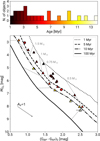 |
Fig. 6 Top panel: histogram of ages estimated for our sample. Bottom: extinction-corrected CMD. The isochrones from PARSEC for 1, 5, 10, and 100 Myr are shown in thick black lines for reference. Thin dotted grey lines connect the points with the same mass in each isochrone ranging from 0.5 M⊙ to 1.5 M⊙. In both panels, colour is used to indicate individual ages. |
5 Summary and conclusions
In this study, we have investigated the low-mass stellar population associated with the FZ CMa system. This region lies between two concentrations with different ages: one group with stars typically older than 10 Myr and another younger than 5 Myr. Therefore, this region was previously suggested to have a mixed-age population.
To verify this hypothesis, our team acquired multi-object spectroscopic data from more than a hundred objects using the Gemini-South Telescope. By identifying Hα emission and Li I absorption (λ 6708 Å) lines, we found 29 TTs, 20 of which are X-ray counterparts. We confirmed the youth of 23 objects previously studied in the literature and discovered 6 TTs that are new members.
We employed two different methods to determine spectral types: (i) comparison with template spectra, accounting for extinction, and (ii) spectral index measurements. By comparing the Hα emission with criteria proposed by White & Basri (2003) and Barrado y Navascués & Martín (2003), we found three CTTs and 18 WTTs. This yields a fraction of nCTT/nWTT = 10%. Previous results from the literature indicate only two Class II objects, one Class II/III, and seven Class III. No WISE classification is available for the remaining sources.
The youth in our sample was indicated by the presence of Li I (λ 6708 Å) in the spectra. A mean age of ![Mathematical equation: $\[8.1_{-3.8}^{+2.1}\]$](/articles/aa/full_html/2026/03/aa57046-25/aa57046-25-eq9.png) Myr was estimated for the whole group using an artificial neural network model. It correlates Li I equivalent width with the effective temperature of the stars to further infer the group’s age. On the other hand, a CMD compared Gaia DR3 photometric data with theoretical models from PARSEC. It revealed a spread in ages, with stars mainly distributed from ~1 to 14 Myr.
Myr was estimated for the whole group using an artificial neural network model. It correlates Li I equivalent width with the effective temperature of the stars to further infer the group’s age. On the other hand, a CMD compared Gaia DR3 photometric data with theoretical models from PARSEC. It revealed a spread in ages, with stars mainly distributed from ~1 to 14 Myr.
It is important to consider whether the stated ages and age spreads are realistic. As has been discussed by Pecaut & Mamajek (2016), evolutionary models often underperform in reproducing parameters for M-type stars, for instance. Moreover, as was discussed by Soderblom et al. (2014), for stars ≲20 Myr, model-dependent and observational uncertainties increase significantly, making it very difficult to estimate reliable absolute ages. In this context, the ages derived here should be regarded as indicators rather than precise absolute values.
Comparing the FZ CMa’s group with clusters of similar age, we found a CTT fraction consistent with what would be expected for the fraction of accreting stars (Fedele et al. 2010; Delfini et al. 2025). This is the opposite of what is observed in the region associated with Z CMa, where Fernandes et al. (2015) found a lower than expected CTT fraction of 17–24% despite a mean age of 1–2 Myr. However, our sample is very limited, and additional data are needed to draw reliable conclusions about it.
The projected spatial distribution of TTs, combined with age estimates, supports a scenario in which the SN events played a minor role in triggering star formation near FZ CMa. Instead, we identified an older, spatially dispersed population and a younger group concentrated near Sh 2-295. The latter may have formed due to localised triggering by the expanding H II region Sh 2-295.
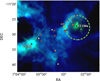 |
Fig. 7 WISE two colour composite: blue is W3, and green is W4. The dashed green circle indicates Sh 2-295 as in Fig. 1. Symbol shapes are the same as in Figs. 4 and 5, while colours follow the age scale from Fig. 6. FZ CMa and Z CMa are shown as a reference. The FoV is the same as in the top panel of the Fig. 1. |
Acknowledgements
We acknowledge the São Paulo Research Foundation (FAPESP) for the financial support (grants #2022/09374-0, #2023/08726-2). This study was financed in part by the Coordenação de Aperfeiçoamento de Pessoal de Nível Superior – Brasil (CAPES) – Finance Code 001. We also thank Rodrigo Carrasco for helping with data reduction of the GMOS spectra. Based on observations obtained at the international Gemini Observatory, a program of NSF NOIRLab, which is managed by the Association of Universities for Research in Astronomy (AURA) under a cooperative agreement with the U.S. National Science Foundation on behalf of the Gemini Observatory partnership: the U.S. National Science Foundation (United States), National Research Council (Canada), Agencia Nacional de Investigaci¡n y Desarrollo (Chile), Ministerio de Ciencia, Tecnología e Innovaci¡n (Argentina), Ministério da Ciência, Tecnologia, Inovações e Comunicações (Brazil), and Korea Astronomy and Space Science Institute (Republic of Korea). This publication makes use of data products from the Two Micron All Sky Survey, which is a joint project of the University of Massachusetts and the Infrared Processing and Analysis Center/California Institute of Technology, funded by the National Aeronautics and Space Administration and the National Science Foundation. This publication makes use of data products from the Wide-field Infrared Survey Explorer, which is a joint project of the University of California, Los Angeles, and the Jet Propulsion Laboratory/California Institute of Technology, funded by the National Aeronautics and Space Administration. The Digitized Sky Survey was produced at the Space Telescope Science Institute under U.S. Government grant NAG W–2166. The images of these surveys are based on photographic data obtained using the Oschin Schmidt Telescope on Palomar Mountain and the UK Schmidt Telescope. The plates were processed into the present compressed digital form with the permission of these institutions. This work has made use of data from the European Space Agency (ESA) mission Gaia (https://www.cosmos.esa.int/gaia), processed by the Gaia Data Processing and Analysis Consortium (DPAC, https://www.cosmos.esa.int/web/gaia/dpac/consortium). Funding for the DPAC has been provided by national institutions, in particular the institutions participating in the Gaia Multilateral Agreement. This work has made use of the VizieR catalogue access tool, Aladin sky atlas, and SIMBAD database operated at CDS, Strasbourg Astronomical Observatory, France. Software: Dustmaps (Green 2018), IRAF (Tody 1986), Numpy (Harris et al. 2020), Pandas (Wes McKinney 2010), Matplotlib (Hunter 2007), Scipy (Virtanen et al. 2020), Astropy (Astropy Collaboration 2022, 2018, 2013), dust_extinction (Gordon 2024), TOPCAT (Taylor 2005), Stilts (Taylor 2006).
References
- Alcalá, J. M., Covino, E., Melo, C., & Sterzik, M. F. 2002, A&A, 384, 521 [NASA ADS] [CrossRef] [EDP Sciences] [Google Scholar]
- Anderson, L. D., Bania, T. M., Balser, D. S., et al. 2014, ApJS, 212, 1 [Google Scholar]
- Andrae, R., Fouesneau, M., Sordo, R., et al. 2023, A&A, 674, A27 [CrossRef] [EDP Sciences] [Google Scholar]
- Astropy Collaboration (Robitaille, T. P., et al.) 2013, A&A, 558, A33 [NASA ADS] [CrossRef] [EDP Sciences] [Google Scholar]
- Astropy Collaboration (Price-Whelan, A. M., et al.) 2018, AJ, 156, 123 [Google Scholar]
- Astropy Collaboration (Price-Whelan, A. M., et al.) 2022, ApJ, 935, 167 [NASA ADS] [CrossRef] [Google Scholar]
- Barrado y Navascués, D., & Martín, E. L. 2003, AJ, 126, 2997 [Google Scholar]
- Bressan, A., Marigo, P., Girardi, L., et al. 2012, MNRAS, 427, 127 [NASA ADS] [CrossRef] [Google Scholar]
- Cardelli, J. A., Clayton, G. C., & Mathis, J. S. 1989, ApJ, 345, 245 [Google Scholar]
- Chen, Y., Girardi, L., Bressan, A., et al. 2014, MNRAS, 444, 2525 [Google Scholar]
- Chen, Y., Bressan, A., Girardi, L., et al. 2015, MNRAS, 452, 1068 [Google Scholar]
- Chen, X., Wang, S., Deng, L., et al. 2020, ApJS, 249, 18 [NASA ADS] [CrossRef] [Google Scholar]
- Claes, R. A. B., Campbell-White, J., Manara, C. F., et al. 2024, A&A, 690, A122 [NASA ADS] [CrossRef] [EDP Sciences] [Google Scholar]
- Comeron, F., Torra, J., & Gomez, A. E. 1998, A&A, 330, 975 [NASA ADS] [Google Scholar]
- Cushing, M. C., Marley, M. S., Saumon, D., et al. 2008, ApJ, 678, 1372 [NASA ADS] [CrossRef] [Google Scholar]
- Delfini, L., Vioque, M., Ribas, Á., & Hodgkin, S. 2025, A&A, 699, A145 [NASA ADS] [CrossRef] [EDP Sciences] [Google Scholar]
- Dobashi, K. 2011, PASJ, 63, S1 [NASA ADS] [CrossRef] [Google Scholar]
- Dobashi, K., Marshall, D. J., Shimoikura, T., & Bernard, J.-P. 2013, PASJ, 65, 31 [NASA ADS] [Google Scholar]
- Dong, Y., Xu, Y., Hao, C., et al. 2024, AJ, 168, 225 [Google Scholar]
- Earl, N., Tollerud, E., O’Steen, R., et al. 2025, astropy/specutils: v2.1.0 [Google Scholar]
- Fedele, D., van den Ancker, M. E., Henning, T., Jayawardhana, R., & Oliveira, J. M. 2010, A&A, 510, A72 [NASA ADS] [CrossRef] [EDP Sciences] [Google Scholar]
- Fernandes, B., Gregorio-Hetem, J., Montmerle, T., & Rojas, G. 2015, MNRAS, 448, 119 [Google Scholar]
- Fernandes, B., Montmerle, T., Santos-Silva, T., & Gregorio-Hetem, J. 2019, A&A, 628, A44 [NASA ADS] [CrossRef] [EDP Sciences] [Google Scholar]
- Fischer, W. J., Padgett, D. L., Stapelfeldt, K. L., & Sewiło, M. 2016, ApJ, 827, 96 [NASA ADS] [CrossRef] [Google Scholar]
- Fitzpatrick, E. L. 1999, PASP, 111, 63 [Google Scholar]
- Gaia Collaboration (Vallenari, A., et al.) 2023, A&A, 674, A1 [NASA ADS] [CrossRef] [EDP Sciences] [Google Scholar]
- Gordon, K. 2024, J. Open Source Softw., 9, 7023 [NASA ADS] [CrossRef] [Google Scholar]
- Gordon, K. D., Clayton, G. C., Decleir, M., et al. 2023, ApJ, 950, 86 [CrossRef] [Google Scholar]
- Green, G. M. 2018, J. Open Source Softw., 3, 695 [Google Scholar]
- Green, G. M., Schlafly, E., Zucker, C., Speagle, J. S., & Finkbeiner, D. 2019, ApJ, 887, 93 [NASA ADS] [CrossRef] [Google Scholar]
- Gregorio-Hetem, J. 2008, in Handbook of Star Forming Regions, Volume II, 5, ed. B. Reipurth, 1 [Google Scholar]
- Gregorio-Hetem, J., Montmerle, T., Rodrigues, C. V., et al. 2009, A&A, 506, 711 [CrossRef] [EDP Sciences] [Google Scholar]
- Gregorio-Hetem, J., Navarete, F., Hetem, A., et al. 2021, AJ, 161, 133 [NASA ADS] [CrossRef] [Google Scholar]
- Harris, C. R., Millman, K. J., van der Walt, S. J., et al. 2020, Nature, 585, 357 [NASA ADS] [CrossRef] [Google Scholar]
- He, Z., Wang, K., Luo, Y., et al. 2022, ApJS, 262, 7 [NASA ADS] [CrossRef] [Google Scholar]
- Herbst, W., & Assousa, G. E. 1977, ApJ, 217, 473 [NASA ADS] [CrossRef] [Google Scholar]
- Herczeg, G. J., & Hillenbrand, L. A. 2014, ApJ, 786, 97 [Google Scholar]
- Hunter, J. D. 2007, Comput. Sci. Eng., 9, 90 [NASA ADS] [CrossRef] [Google Scholar]
- Jeffries, R. D., Oliveira, J. M., Naylor, T., Mayne, N. J., & Littlefair, S. P. 2007, MNRAS, 376, 580 [NASA ADS] [CrossRef] [Google Scholar]
- Jeffries, R. D., Jackson, R. J., Wright, N. J., et al. 2023, MNRAS, 523, 802 [NASA ADS] [CrossRef] [Google Scholar]
- Le Borgne, J. F., Bruzual, G., Pell¡, R., et al. 2003, A&A, 402, 433 [CrossRef] [EDP Sciences] [Google Scholar]
- Luhman, K. L., Herrmann, K. A., Mamajek, E. E., Esplin, T. L., & Pecaut, M. J. 2018, AJ, 156, 76 [Google Scholar]
- Mallick, K. K., Ojha, D. K., Samal, M. R., et al. 2012, ApJ, 759, 48 [Google Scholar]
- Manjavacas, E., Lodieu, N., Béjar, V. J. S., et al. 2020, MNRAS, 491, 5925 [NASA ADS] [CrossRef] [Google Scholar]
- Marigo, P., Girardi, L., Bressan, A., et al. 2017, ApJ, 835, 77 [Google Scholar]
- Martin, E. L., Montmerle, T., Gregorio-Hetem, J., & Casanova, S. 1998, MNRAS, 300, 733 [Google Scholar]
- Merino, B., Placco, V., & Stanghellini, L. 2022, The NOIRLab Mirror, 3, 13 [Google Scholar]
- O’Donnell, J. E. 1994, ApJ, 422, 158 [Google Scholar]
- Pastorelli, G., Marigo, P., Girardi, L., et al. 2019, MNRAS, 485, 5666 [Google Scholar]
- Pastorelli, G., Marigo, P., Girardi, L., et al. 2020, MNRAS, 498, 3283 [Google Scholar]
- Pecaut, M. J., & Mamajek, E. E. 2013, ApJS, 208, 9 [Google Scholar]
- Pecaut, M. J., & Mamajek, E. E. 2016, MNRAS, 461, 794 [Google Scholar]
- Pérez Paolino, F., Bary, J. S., Hillenbrand, L. A., Horner, B., & Carvalho, A. 2025, ApJ, 990, 205 [Google Scholar]
- Pettersson, B., & Reipurth, B. 2019, A&A, 630, A90 [NASA ADS] [CrossRef] [EDP Sciences] [Google Scholar]
- Santos-Silva, T., Gregorio-Hetem, J., Montmerle, T., Fernandes, B., & Stelzer, B. 2018, A&A, 609, A127 [NASA ADS] [CrossRef] [EDP Sciences] [Google Scholar]
- Santos-Silva, T., Perottoni, H. D., Almeida-Fernandes, F., et al. 2021, MNRAS, 508, 1033 [NASA ADS] [CrossRef] [Google Scholar]
- Sharpless, S. 1959, ApJS, 4, 257 [Google Scholar]
- Shevchenko, V. S., Ezhkova, O. V., Ibrahimov, M. A., van den Ancker, M. E., & Tjin A Djie, H. R. E. 1999, MNRAS, 310, 210 [Google Scholar]
- Skrutskie, M. F., Cutri, R. M., Stiening, R., et al. 2006, AJ, 131, 1163 [NASA ADS] [CrossRef] [Google Scholar]
- Soderblom, D. R., Hillenbrand, L. A., Jeffries, R. D., Mamajek, E. E., & Naylor, T. 2014, in Protostars and Planets VI, eds. H. Beuther, R. S. Klessen, C. P. Dullemond, & T. Henning, 219 [Google Scholar]
- Stanghellini, L., Magrini, L., Casasola, V., & Villaver, E. 2014, A&A, 567, A88 [NASA ADS] [CrossRef] [EDP Sciences] [Google Scholar]
- Tang, J., Bressan, A., Rosenfield, P., et al. 2014, MNRAS, 445, 4287 [NASA ADS] [CrossRef] [Google Scholar]
- Taylor, M. B. 2005, in Astronomical Society of the Pacific Conference Series, 347, Astronomical Data Analysis Software and Systems XIV, eds. P. Shopbell, M. Britton, & R. Ebert, 29 [Google Scholar]
- Taylor, M. B. 2006, in Astronomical Society of the Pacific Conference Series, 351, Astronomical Data Analysis Software and Systems XV, eds. C. Gabriel, C. Arviset, D. Ponz, & S. Enrique, 666 [Google Scholar]
- Tody, D. 1986, SPIE Conf. Ser., 627, 733 [Google Scholar]
- Ushomirsky, G., Matzner, C. D., Brown, E. F., et al. 1998, ApJ, 497, 253 [NASA ADS] [CrossRef] [Google Scholar]
- Virtanen, P., Gommers, R., Oliphant, T. E., et al. 2020, Nat. Methods, 17, 261 [Google Scholar]
- Weaver, G., Jeffries, R. D., & Jackson, R. J. 2024, MNRAS, 534, 2014 [Google Scholar]
- Wes McKinney 2010, in Proceedings of the 9th Python in Science Conference, eds. S. van der Walt, & J. Millman, 56 [Google Scholar]
- White, R. J., & Basri, G. 2003, ApJ, 582, 1109 [Google Scholar]
- Wright, E. L., Eisenhardt, P. R. M., Mainzer, A. K., et al. 2010, AJ, 140, 1868 [Google Scholar]
IRAF is distributed by the National Optical Astronomy Observatory, which is operated by the Association of Universities for Research in Astronomy, Inc., under cooperative agreement with the National Science Foundation.
US National Gemini Office 2022, GMOS Data Reduction Cookbook (Version 2.0; Tucson: NSF’s National Optical-Infrared Astronomy Research Laboratory), available online at: https://noirlab.edu/science/programs/csdc/usngo/gmos-cookbook/
Re-normalised unit weight error.
Appendix A Spectra of the TTs in the GMOS sample
Here we present portions of the spectra of the remaining 28 TTs not shown previously in the main text, focussing on the spectral regions around Hα, Li I (λ 6708 Å) and Ca I (λ 6718 Å) features.
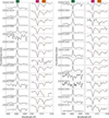 |
Fig. A.1 GMOS spectra of 28 TTs identified in this work. The Hα, Li I (λ 6708 Å) and Ca I (λ 6718 Å) features are highlighted. Each object is labelled with its 2MASS identifier. An artefact is present near the Ca I line in the spectrum of 2MASS J07025410-1125160. |
Appendix B List of additional Hα emitters
In this appendix, we present a list of objects with Hα emission, but without detectable Li I absorption. The six sources found are shown in Table B.1. One of them does not have an IR counterpart in the 2MASS catalogue, considering 1″ maximum separation.
None of them are in the lists of members previously determined by our team (Santos-Silva et al. 2021; Gregorio-Hetem et al. 2021), and only one was previously found in the survey for Hα emission conducted by Pettersson & Reipurth (2019) – object 07031171-1135369, which also shows the highest Hα emission among these six objects. These sources may be dMe stars; however, further investigation is required.
Hα emitters without Li absorption line.
Appendix C Extinction
We compared our extinction estimates, obtained from spectral fitting, with estimates from two-dimensional maps: one from Cambrésy (private communication), and another one from Dobashi (2011) and Dobashi et al. (2013), hereafter Dobashi+ (Fig. C.1). The resolution of these maps varies between 1′ and 12′. We also used a three-dimensional map (Bayestar19 – Green et al. 2019) with a typical scale of 3′ 4–13′ 7, as well as the estimates from Gaia DR3 – General Stellar Parametrizer from Photometry (GSP-Phot, Andrae et al. 2023).
None of the literature extinction values showed good agreement, either among themselves or with our values (Fig. C.2). The Spearman correlation coefficient between the distributions typically ranges from −0.08 to 0.2, indicating very weak or negligible correlations. The only exceptions are between this work and GSP-Phot, which yields a higher correlation (Spearman ~ 0.7), and between Dobashi+ and Cambrésy (Spearman ~0.6). Although our extinction values were rounded to 0.25 mag steps, this does not seem to explain the discrepancies. One possibility is that since the 2D and 3D maps cannot resolve individual stars, they do not represent the exact line-of-sight values for each star. In particular, the 2D maps do not take into account the distance to each object, which is important to objects that are not deeply embedded in the molecular clouds. Considering that the AV values of this work tend to be lower than the AV maps, we suggest that our sample is mainly found in the borders of the clouds, as can be noted in Fig C.1. On the other hand, GSP-Phot does not account for different physical process that happens in PMS, such as accretion. There is also a degeneracy between GSP-Phot temperature and extinction estimates (Andrae et al. 2023) which is another possible reason for the differences found.
Figure C.3 shows the amplitude of the extinction for each TTs in our sample. For approximately 55% of the sources, our estimates are lower than all the literature values. Conversely, our values are very conservative in most cases. Notably, the extinction distribution adopted here provides the best agreement with theoretical models in the CMD (Fig. 6). These results indicate that poor agreement among the extinction estimates is mainly due to differences in the adopted methods rather than wrong spectral type allocation.
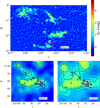 |
Fig. C.1 2D extinction maps from Dobashi+ and Cambrésy. The top panel indicates the CMa region while the bottom panel shows a zoom in the region highlighted in magenta in the top panel. Magenta star symbols indicate the position of all 29 TT stars studied in this work. |
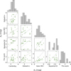 |
Fig. C.2 Comparison of extinction estimates for the TTs identified in this work with values from the literature. |
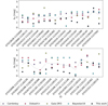 |
Fig. C.3 Visual extinction estimates for each TTs (identified by the 2MASS id) from different methods. |
Appendix D Spectral type estimates using different methodologies
Table D.1 lists the spectral types derived for each source using different methods (mentioned in Sect. 3.2) along with the final adopted values.
Different estimates of spectral type.
All Tables
All Figures
|
Fig. 1 Top panel: optical (Digitized Sky Survey – DSS2, F+R) image of the region studied in this work. The black squares indicate the GMOS 1–4 fields of Table 1. The dashed green circle shows the Sh 2-295 H II region (Sharpless 1959). Bottom panel: GMOS R pre-images used to prepare GMOS masks. To facilitate the identification of the co-ordinate system orientation in each image, the grid lines corresponding to RA and Dec are plotted in grey as dashed and solid lines, respectively. The position of the slits are shown by open blue squares. In both panels, orange lines represent AV = 1 and AV = 3 mag contours (Cambrésy, priv. commun.) and open magenta circles indicate X-ray sources (Santos-Silva et al. 2018). Note that not all X-ray sources were covered by the GMOS observations. |
| In the text | |
|
Fig. 2 Example of a GMOS spectrum highlighting Hα emission, and Li I (λ6708 Å) and Ca I (λ6718 Å) absorption features. The top right panel shows the angular position of a TTs (green circle) compared to X-ray sources (black circles – Santos-Silva et al. 2018), confirming it as an X-ray counterpart. |
| In the text | |
|
Fig. 3 Example of spectral typing via spectral comparison. The GMOS spectrum, normalised by the flux at 7050 Å, is shown in black in the regions used to calculated G and in grey elsewhere. The pair AV = 0.75 mag, and M2-type stellar spectrum (green line) represents the best fit to the object. For comparison, spectra of M-1 and M-3 type stars are shown in blue and orange, respectively. The bottom panel shows the residuals of the comparison between the GMOS object and the M2-type stellar spectrum. |
| In the text | |
|
Fig. 4 Thresholds defining the CTT classification following White & Basri green dashed line (2003) and Barrado y Navascués & Martín orange dash-dotted line (2003). Blue symbols represent our sample; grey symbols are data from Fernandes et al. (2015). These criteria were used to classify the CTTs (indicated by circles), WTTs (triangles), and possible WTTs (crosses). |
| In the text | |
|
Fig. 5 W(Li) from the 6708 Å line vs Teff and spectral type. Symbols and colours are the same as in Fig. 4. Grey lines are polynomial fits for observed data in other young clusters: Sco-Cen (10–16 Myr), IC2602 (45 Myr), and Pleiades (125 Myr) – see Pecaut & Mamajek (2016) and references therein. The orange line represents the expected curve for a population of |
| In the text | |
|
Fig. 6 Top panel: histogram of ages estimated for our sample. Bottom: extinction-corrected CMD. The isochrones from PARSEC for 1, 5, 10, and 100 Myr are shown in thick black lines for reference. Thin dotted grey lines connect the points with the same mass in each isochrone ranging from 0.5 M⊙ to 1.5 M⊙. In both panels, colour is used to indicate individual ages. |
| In the text | |
|
Fig. 7 WISE two colour composite: blue is W3, and green is W4. The dashed green circle indicates Sh 2-295 as in Fig. 1. Symbol shapes are the same as in Figs. 4 and 5, while colours follow the age scale from Fig. 6. FZ CMa and Z CMa are shown as a reference. The FoV is the same as in the top panel of the Fig. 1. |
| In the text | |
|
Fig. A.1 GMOS spectra of 28 TTs identified in this work. The Hα, Li I (λ 6708 Å) and Ca I (λ 6718 Å) features are highlighted. Each object is labelled with its 2MASS identifier. An artefact is present near the Ca I line in the spectrum of 2MASS J07025410-1125160. |
| In the text | |
|
Fig. C.1 2D extinction maps from Dobashi+ and Cambrésy. The top panel indicates the CMa region while the bottom panel shows a zoom in the region highlighted in magenta in the top panel. Magenta star symbols indicate the position of all 29 TT stars studied in this work. |
| In the text | |
|
Fig. C.2 Comparison of extinction estimates for the TTs identified in this work with values from the literature. |
| In the text | |
|
Fig. C.3 Visual extinction estimates for each TTs (identified by the 2MASS id) from different methods. |
| In the text | |
Current usage metrics show cumulative count of Article Views (full-text article views including HTML views, PDF and ePub downloads, according to the available data) and Abstracts Views on Vision4Press platform.
Data correspond to usage on the plateform after 2015. The current usage metrics is available 48-96 hours after online publication and is updated daily on week days.
Initial download of the metrics may take a while.