| Issue |
A&A
Volume 707, March 2026
|
|
|---|---|---|
| Article Number | A52 | |
| Number of page(s) | 16 | |
| Section | Extragalactic astronomy | |
| DOI | https://doi.org/10.1051/0004-6361/202557687 | |
| Published online | 25 February 2026 | |
Black holes in the shadows: The missing high-ionization lines in the earliest JWST active galactic nuclei
1
Dipartimento di Fisica “G. Occhialini”, Università degli Studi di Milano-Bicocca Piazza della Scienza 3 I-20126 Milano, Italy
2
Stockholm University, Department of Astronomy and Oskar Klein Centre for Cosmoparticle Physics AlbaNova University Centre SE-10691 Stockholm, Sweden
3
Kavli Institute for Cosmology, University of Cambridge Madingley Road Cambridge CB3 0HA, UK
4
Department of Astronomy & Astrophysics, University of California Santa Cruz 1156 High Street Santa Cruz CA 95064, USA
5
Cavendish Laboratory, University of Cambridge 19 JJ Thomson Avenue Cambridge CB3 0HE, UK
6
Department of Physics and Astronomy, University College London Gower Street London WC1E 6BT, UK
7
Waseda Research Institute for Science and Engineering, Faculty of Science and Engineering, Waseda University, 3-4-1 Okubo Shinjuku Tokyo 169-8555, Japan
★ Corresponding author: This email address is being protected from spambots. You need JavaScript enabled to view it.
Received:
14
October
2025
Accepted:
15
December
2025
Abstract
Observations with the James Webb Space Telescope (JWST) have uncovered a substantial population of high-redshift, broad-line active galactic nuclei (AGNs), whose properties challenge standard models of black-hole growth and AGN emission. We analyzed a spectroscopic sample of 34 Type 1 AGNs from the JWST Advanced Deep Survey (JADES) survey, spanning redshifts 1.7 < z < 9, to constrain the physical nature of the accretion flows powering these sources with broad-line diagnostics statistically for the first time. At z > 5, we find a marked suppression of high-ionization emission lines (HeII, CIV, NV) relative to prominent broad Hα and narrow [OIII] features. This contrast places strong constraints on the shape of the ionizing spectral energy distribution (SED) and on the physical conditions in the broad-line region (BLR). By comparing the observations to photoionization models based on SEDs of black holes accreting at sub-Eddington ratios, we show that standard AGN continua struggle to reproduce the observed broad-line ratios and equivalent widths (EWs) across a wide ionization parameter range. These results suggest the need for modified SEDs – either intrinsically softened due to super-Eddington accretion or radiative inefficiencies in the innermost disk, or externally filtered by intervening optically thick gas that absorbs or scatters the highest energy photons before they reach the BLR.
Key words: galaxies: active / galaxies: formation / galaxies: high-redshift / quasars: emission lines / quasars: supermassive black holes
© The Authors 2026
 Open Access article, published by EDP Sciences, under the terms of the Creative Commons Attribution License (https://creativecommons.org/licenses/by/4.0), which permits unrestricted use, distribution, and reproduction in any medium, provided the original work is properly cited.
This article is published in open access under the Subscribe to Open model. This email address is being protected from spambots. You need JavaScript enabled to view it. to support open access publication.
1. Introduction
Deep-field observations with the James Webb Space Telescope (JWST) have identified a substantial population of moderate-luminosity (Lbol ∼ 1043–1045 erg s−1), broad-line active galactic nuclei (AGNs) at redshifts z > 4 – with the full width at half maximum (FWHM) of broad Balmer lines usually being 1000–6000 km s−1 – with number densities that are nearly 100 times higher than those of ultraviolet (UV) -selected quasars at similar epochs (e.g., Harikane et al. 2023; Juodžbalis et al. 2025a). These AGNs are powered by accretion onto early massive black holes (MBHs) that appear overmassive with respect to the local black-hole-mass – stellar-mass relation (e.g., Cohn et al. 2025; Harikane et al. 2023; Kocevski et al. 2023; see also Geris et al. 2026). They also show unusually weak X-ray emission (e.g., Ananna et al. 2024; Kokubo & Harikane 2025; Maiolino et al. 2025; Yue et al. 2024; Sacchi & Bogdán 2025); faint high-ionization lines (Lambrides et al. 2024; Juodžbalis et al. 2025a; Wang et al. 2025), with only a few outliers reported by Tang et al. (2025); and in some cases Balmer line-absorption features (especially for those classified as “little red dots” (LRDs); e.g., Matthee et al. 2024; Juodžbalis et al. 2024; Kocevski et al. 2025; Ji et al. 2025; D’Eugenio et al. 2026; D’Eugenio et al. 2025b) that are suggestive of large column densities of neutral hydrogen in the nuclear region (e.g., Juodžbalis et al. 2024; Inayoshi & Maiolino 2025; Ji et al. 2025; de Graaff et al. 2025; Naidu et al. 2025; Taylor et al. 2025; D’Eugenio et al. 2025c). These properties present substantial challenges to current theories of MBH growth and the nature of broad-line AGNs at high redshift.
Rest-frame UV-optical emission lines in AGN spectra are highly sensitive diagnostics of the shape of the SED, particularly the part of the SED in the far-ultraviolet (FUV), extreme ultraviolet (EUV), and soft X-ray bands – wavelength ranges that are largely inaccessible due to interstellar and intergalactic absorption (e.g., Osterbrock & Ferland 2006). Variations in line ratios and equivalent widths (EWs) encode information about the physical conditions in the line-emitting gas, including ionization parameter, metallicity, covering factor, geometry, and – crucially – the Eddington ratio λEdd = Ṁ/ṀEdd and black-hole mass (Boroson & Green 1992; Ferland et al. 2020). The degeneracies inherent in this mapping have historically limited the diagnostic power of photoionization models, particularly due to the poorly constrained shape of the ionizing continuum between the Lyman limit and ∼ 0.3 keV (e.g., Done et al. 2012).
Recent advances in SED templates for sub-Eddington and super-Eddington accretion flows have enabled a more quantitative comparison between predicted and observed emission line trends (e.g., Capellupo et al. 2015; Hall et al. 2018; Kubota & Done 2019). Some of these models also incorporate geometric effects and the anisotropic radiation fields inherent to supercritical accretion flows (e.g., Wang et al. 2014; Pacucci & Narayan 2024; Madau & Haardt 2024; Madau 2025). Although bolometric luminosities and black-hole masses inferred from deep JWST surveys typically suggest sub-Eddington accretion rates for the general population of AGNs at z ≳ 4 (e.g., Maiolino et al. 2024; Juodžbalis et al. 2025a), large uncertainties in virial mass estimates as well as bolometric conversions, particularly at high redshift, leave the Eddington ratio poorly constrained (e.g., Lupi et al. 2024; Bertemes et al. 2025). There are only a few cases in which the black-hole masses were not measured through the single-epoch method, but more directly through dynamics in z > 2 AGNs, revealing both super-Eddington accretions (in a few luminous quasars; e.g., Abuter et al. 2024), and sub-Eddington accretions (in the case of a lensed LRD at z = 7, Juodžbalis et al. 2025b).
The anomalies observed in JWST AGNs raise key questions about the shape of the ionizing continuum, the structure and physical conditions of the BLR, and the nature of radiative transfer in early AGNs. The marked deficiency of high-ionization emission lines suggests a significant departure from the standard AGN photoionization paradigm. Two primary scenarios may account for this: either the ionizing SEDs are intrinsically soft or filtered, reducing the photon flux at energies ≳50 eV; or the AGNs are accreting in a super-Eddington regime, where geometric effects, inner obscuration, and radiation collimation lead to anisotropic emission and the selective suppression of high-ionization lines (Madau 2025). These possibilities carry important implications for the physical state of the BLR and the fueling mechanisms of early black holes.
To investigate the physical origin of the emerging spectroscopic trends in early AGNs, we analyzed a sample of 34 broad-line AGNs from the JWST JADES survey (Bunker et al. 2024; Rieke et al. 2023; Eisenstein et al. 2023; D’Eugenio et al. 2025a) selected by Juodžbalis et al. (2025a), spanning the 1.7 < z < 9 redshift range. Using both prism and grating spectroscopy, we examined rest-frame UV and optical emission-line diagnostics to constrain the ionization structure and continuum hardness across cosmic time. We constructed a grid of photoionization models varying in ionization parameter, gas density, and incident SED shape and compared predicted line ratios and equivalent widths to the observations. Special emphasis is placed on the z > 5 regime, where deviations from local AGN templates seem most pronounced and where constraints on the ionizing continuum are most urgently needed. In this work, we focused on the regime of sub-Eddington accretion and assessed whether standard SEDs representative of nearby AGNs can reproduce the observed line properties. The limitations of these models provide a benchmark for future investigations of super-Eddington accretion and SED filtering scenarios, which will be explored in a forthcoming paper.
2. Sample selection
We constructed our sample from the Type 1 AGNs selected by Juodžbalis et al. (2025a), which used JWST NIRSpec medium resolution spectra (R ∼ 1000) for identifications of BLR emission. Emission lines were fit using multiple Gaussian components to distinguish narrow-line emission from star formation or the narrow-line region, and broad emission from high-velocity virialized gas near the black hole. Hα was used as the primary tracer due to its high luminosity and visibility in JWST spectra over z ∼ 0.5 − 7.
In the following, we summarize the identification and selection criteria as performed by Juodžbalis et al. (2025a). In their analysis, for each source, the Hα + [NII] emission complex was fit with two models: one model with only narrow Hα and [NII] λλ6548,6583 emission (constrained to share velocity and width, with the [NII] doublet ratio fixed at 3), and the other model with an additional broad Hα component. Markov chain Monte Carlo (MCMC) sampling was used to fit parameters. The same method was applied to [OIII] λλ4959,5007 and Hβ to identify any ionized outflows and estimate dust attenuation via the Balmer decrement. In cases with significant outflow features, Hα was refit including an outflow component with priors derived from [OIII] to distinguish outflows from the BLR. Since BLRs do not have [OIII] emission, excess broad wings in Hα lacking [OIII] support were attributed to the BLR. Within the JADES sample, four sources require further analyses as noted by Juodžbalis et al. (2025a). These are listed below:
-
GN-200679 (z = 4.547) lacked [OIII] coverage in its NIRSpec spectra, so the broad Hα identified may also trace an outflow – it is thus flagged as tentative;
-
GN-23924 (z = 1.676) showed a weak BLR compared to outflows, also marked tentative;
-
GS-49729 (z = 3.189) and GS-159717 (z = 5.077) exhibited complex broad-line profiles only well fit with two Gaussians or an exponential model, with GS-159717 further requiring a strong rest-frame absorption component (Juodžbalis et al. 2025a; D’Eugenio et al. 2026). The complex profile potentially reflects non-Gaussian BLR kinematics (Kollatschny & Zetzl 2013), unresolved black-hole binaries (Maiolino et al. 2024), or radiative-transfer effects (Laor 2006; Rusakov et al. 2025; see, however, Brazzini et al. 2025 for a counterargument). For consistency, the two broad components were combined into a single one to estimate FWHM and luminosity.
Using the methodology described above, a total of 30 Type 1 AGNs were identified by Juodžbalis et al. (2025a), with 28 robust identifications based on the presence of a broad Hα component with a signal-to-noise ratio (S/N) > 5, and two tentative identifications that narrowly miss one of the selection thresholds. To compare the goodness-of-fit of models with and without a broad component, they also used the Bayesian information criterion (BIC) with ΔBIC > 5, which penalizes model complexity and is defined as BIC = χ2 + klnn, with k the number of free parameters and n the number of data points.
Visual inspections of the low-resolution NIRSpec/prism spectra (R ∼ 100) led to the identification of four additional Type 1 AGNs at 7 < z < 9 (GN-4685, GS-20030333, GS-20057765, GS-164055) showing hints of broad Hβ emission. While individually these sources did not meet formal significance thresholds, their stacked spectrum, weighted by inverse variance, revealed a statistically significant broad Hβ component. This detection was confirmed via jackknife resampling, and we include it following Juodžbalis et al. (2025a) for completeness. Therefore, these four objects were added to the Type 1 sample, raising the total number AGNs to 34 spanning the 1.7 < z < 9 redshift range. The sample is twice as large as that used in the JWST AGN SED study by Lambrides et al. (2024) and spans a nominal black-hole mass range of MBH ∼ 106–109 M⊙ and Eddington ratios from 0.02 to 0.4; these were derived from single-epoch virial black-hole mass estimates and bolometric luminosities based on Hα as described by Juodžbalis et al. (2025a) following the relation provided by Reines & Volonteri (2015). However, as we show later, despite the moderate nominal λEdd for the bulk of our sample, standard sub-Eddington SEDs do not provide a satisfactory fit to the observed emission.
Notably, all of these AGNs, except GS-49729 and GS-209777, are not detected in X-ray at roughly 2–10 keV in the rest frame, implying significant X-ray weakness compared to local AGNs (Maiolino et al. 2025; Juodžbalis et al. 2025a). As we show later, the two X-ray-detected sources also show drastically different broad-line spectra compared to other sources, and they are more similar to local sources. Next, we describe the spectral measurements we made on our sample.
3. Spectral measurements
3.1. Stacking
To better constrain intrinsically weak or low S/N spectral features, we performed spectral stacking across selected redshift intervals. We applied this method to both the low-resolution (R ∼ 100) NIRSpec prism spectra and the medium-resolution (R ∼ 1000) grating spectra within our sample, using the latest data products reduced with the NIRSpec GTO pipeline (see, e.g., Carniani et al. 2024; D’Eugenio et al. 2025a), which incorporates the most recent JWST calibration updates.
As we mentioned, two JADES AGNs (IDs GS-49729 and GS-209777) have X-ray detections, and we excluded them from the stack. Interestingly, they are more similar to X-ray-normal AGNs, or QSOs, in terms of other spectral features as well, with GS-49729 showing an extremely strong CIV line not visible in the rest of the sample, and both sources display QSO-like continua (Juodžbalis et al. 2025a). Their continuum shape would bias the stacked spectrum relative to the X-ray-undetected population studied here. In addition, GS-209777 shows a steeper Balmer decrement in the narrow lines compared to other objects (see Table 2 in Juodžbalis et al. 2025a), suggesting that its spectral properties differ from those of the bulk of the sample.
For the remaining X-ray-undetected sources, each prism/grating spectrum was first shifted to the rest frame using the spectroscopic redshift. The spectra were then resampled onto a common wavelength grid with a 2 Å step for grating and a 5 Å step for prism using SPECTRES (Carnall 2017). The chosen wavelength steps ensure consistent sampling across all spectra, enabling accurate alignment of spectral features and maximizing sensitivity to faint emission lines; using much finer sampling would only amplify noise fluctuations without adding information, whereas coarser sampling would risk smoothing out the spectral features. The stacking wavelength range in each redshift bin was chosen to ensure at least 70% spectral coverage throughout the sample. We found that the prism provides rest-frame UV coverage for all 32 objects, while among the gratings, only G140M sufficiently covers the UV, with 25 out of 32 spectra contributing. In the optical regime, no single grating spans the full range; instead, it is covered in sections by G140M, G235M, and G395M. Therefore, all measurements in the optical range are based on stacks that combine the spectra from these three gratings. Figure 1 shows the rest-frame wavelength coverage of each disperser for all individual targets.
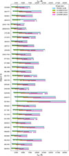 |
Fig. 1. Spectral wavelength coverage across dispersers for each object. Invalid or missing values are masked and shown as empty. The dashed vertical line at 3000 Å indicates a conventional division between the UV and optical regimes, though it is not used in the kinematic classification of emission lines. The treatment of lines near this boundary (e.g., [NeV] λ3426) is discussed in Section 3.2. |
Stacking was performed as an inverse-variance weighted average to maximize S/N, normalized by the flux F[OIII] λ5007, following Isobe et al. (2025). For grating spectra, line fluxes were measured by fitting Gaussian profiles, with uncertainties estimated via Monte Carlo resampling. For prism spectra, where the [OIII] doublet is blended and the low-resolution provides too few points for a reliable Gaussian fit, we measured the flux by direct summation of the continuum-subtracted line profile and derived the [OIII] λ5007 flux by scaling from the total doublet flux; the uncertainty was obtained by summing the per-pixel errors in quadrature over the same interval. The [OIII] flux measured from the prism spectrum was used for normalization when no grating-based measurement was available for a given object. These measurements were used solely for normalization purposes prior to stacking, while the detailed spectral fitting of the stacked spectra is described in Section 3.2. Normalized spectra and their associated normalized uncertainties were combined on a common grid, removing outlier pixels via 5σ clipping. Finally, the stacks and their formal errors were obtained as the inverse-variance weighted mean and the corresponding weighted standard error of the mean, respectively.
During stacking, we divided our sample into three redshift bins (z < 3.5, 3.5 < z < 5, and z > 5). Since, as described above, we stacked the prism, G140M grating, and combined gratings for different spectral ranges and for each redshift bin, we obtained a total of 3 × 3 = 9 stacked spectra, three at R ∼ 100 and six at R ∼ 1000. Figure 2 shows one of the resulting stacked spectra, the others are reported in Appendix B.
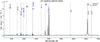 |
Fig. 2. Stack of JWST NIRSpec (G140M+G235M+G395M) grating spectra of JADES Type 1 AGNs in the high-redshift bin (z > 5). For visualization purposed, the normalized stack was multiplied by the mean [OIII] λ5007 flux of the 15 contributing objects; this rescaling is used only for the figure and not for any measurements. |
3.2. Spectral fitting
Building on the resolution-matched stacked spectra, we initiated the spectral fitting process of the stacked spectra to recover emission-line fluxes and kinematics, accounting for instrumental broadening by adopting the MSA line spread function (LSF) for point-like sources from De Graaff et al. (2024), evaluated at the average redshift of the sources in each stack. In the case of mixed grating stacks (G140M+G235M+G395M), where there are three different LSFs, we adopted the LSF of the grating that contributes most to each redshift bin (i.e., G235M as it covers the majority of objects).
We then performed a full-spectrum fitting using a modified version of the Python implementation of the Penalized PiXel-Fitting (pPXF; Cappellari & Emsellem 2004; Cappellari 2017, 2023) method customized for AGN analysis. The observed spectra were modeled as a combination of stellar-continuum templates and emission-line components, with the AGN continuum approximated by high-order Legendre additive polynomials rather than an explicit template (e.g., Marconcini et al. 2025; De Graaff et al. 2025) to optimize the fit of the continua and nebular emission simultaneously. For the stellar continuum, we used templates from the eMILES stellar population synthesis library (Vazdekis et al. 2016), which encompasses a broad range of stellar ages and metallicities, ensuring a realistic representation of stellar absorption features and continuum shapes in the 1680–50 000 Å wavelength range. We modeled emission-line profiles as Gaussians, including narrow emission lines and broader components associated with the BLR. For emission-line doublets that arise from the same upper energy level, the flux ratios are governed by atomic physics and held fixed1. We adopted the theoretical values computed with the PyNeb library (Luridiana et al. 2015), using them as fixed scaling factors during both the construction of the line templates and the measurement of integrated fluxes.
To evaluate emission-line detections, we applied a conservative 3σ threshold based on the formal uncertainties returned by pPXF. A line was considered detected if its integrated flux exceeded three times its uncertainty; otherwise, we report a 3σ upper limit. Integrated fluxes were computed by multiplying the best-fit amplitude of each line by the local spectral dispersion and the continuum normalization factor.
3.2.1. The G140M+G235M+G395M stack
The combined-grating stacked spectra – used for the measurements of optical emission lines – were modeled using additive and multiplicative Legendre polynomials. For the 3.5 < z < 5 and z > 5 stacks, we adopted a sixth-degree additive polynomial together with a second-degree multiplicative polynomial. Since our focus is on emission lines, the continuum modeling serves only as a baseline and is not interpreted physically. For the z < 3.5 stack, however, a higher degree of flexibility was required, and we used a 16th-degree additive polynomial and a fourth-degree multiplicative polynomial. This likely reflects the limited number of spectra contributing to this stack (only five objects), which made it more challenging to constrain the continuum shape. We also allowed for line asymmetry – broad emission lines were modeled with Gauss–Hermite profiles including the h3 and h4 terms, enabling deviations from purely Gaussian symmetric shapes, without attributing them to specific kinematic subcomponents such as outflows. The low-redshift stack demanded this additional freedom, likely due to the smaller sample size and the correspondingly more complex continuum and line profiles.
At this spectral resolution, we created the following three distinct kinematics groups:
-
Narrow components: Hα, Hβ, Hϵ, Hδ, Hγ, [OII] λλ3726,3729, HeI λ3889, [OIII] λ4363, HeII λ4686, HeI λ5876, [NII] λλ6548,6583, [SII] λλ6716,6731.
-
High-ionization narrow components: [NeV] λ3426, [NeIII] λλ3869,3968, [OIII] λλ4959,5007.
-
Broad components: Hα, Hβ, HeII λ4686.
High-ionization narrow lines likely originate closer to the AGN and are more susceptible to the kinematic effects of AGN-driven outflows or turbulent motions within the narrow-line region (NLR) and are generally found to be broader than the other narrow lines (e.g., Spoon & Holt 2009; Dasyra et al. 2011). Both a narrow and a broad HeII λ4686 component were included in the fit to ensure proper constraints on the BLR emission, as both narrow and broad HeII have been observed in JWST/NIRSpec studies of high-redshift AGNs (e.g., Übler et al. 2023), and the presence of a broad HeII feature is commonly observed in luminous Type 1 AGNs (e.g., Marziani et al. 2010). In the meanwhile, the narrow HeII has been proven to be a key diagnostic of EUV photon sources in galaxies and shown to be effective at distinguishing AGN from stellar ionization in low-metallicity environments (e.g., Shirazi & Brinchmann 2012; Katz et al. 2023; Übler et al. 2023; Cleri et al. 2025; Scholtz et al. 2025; Treiber et al. 2025).
Across both prism and grating stacked spectra, broad components were only fit for a restricted set of lines. Although in principle all permitted lines may display a broad component, in practice we limited our analysis to Hα, Hβ, CIV, and HeII. Broad components in other transitions are generally too weak or poorly constrained in our data to yield reliable results, whereas CIV and HeII were nonetheless included since establishing constraints (including upper limits) on these lines is a key goal of this work.
3.2.2. The prism stack
For the prism stacked spectra, we adopted a slightly modified fitting strategy. In this case, we employed a 12th-degree additive polynomial, allowing for line asymmetries to ensure sufficient flexibility. We also tested fits with different levels of high-order polynomials and found that the resulting line fluxes remained stable to within ∼10%.
The broader wavelength coverage of the prism spectra enabled us to fit UV emission lines, which could not be consistently accessed with the gratings except for the G140M stack – with the specific procedures for tying and treating these lines described later in this section. We restricted the fit range of prism-stack spectra to λrest > 1250 Å, thereby excluding the region affected by Lyα and potential damping wings. This conservative cut is motivated by the complex radiative transfer of Lyα photons, which are subject to resonant scattering and significant absorption by the intergalactic medium (IGM). We further divided the sample into the following three distinct kinematic groups:
-
Narrow components: Hα, Hβ, Hϵ, Hδ, Hγ,[OII] λλ3726,3729, [NeIII] λλ3869,3968, HeI λ3889, [OIII] λ4363, HeII λ4686, HeI λ5876, [NII] λλ6548,6583, [SII] λλ6716,6731.
-
UV narrow components: SiII λ1260, SiII λ1304, CIV λ1549, HeII λ1640, SiIII] λ1892, [NeIV] λ2424, OII] λ2471, NV λ1240, OIII] λλ1661,1666, CIII] λλ1907,1909, MgII λ2796, [NeV] λ3426.
-
Broad components: Hα, Hβ, CIV λ1549, HeII λ1640, HeII λ4686.
In this classification, we grouped [NeV] λ3426 with the UV narrow lines. High-ionization UV transitions such as CIV and NV are established tracers of BLR and AGN-driven outflows, often exhibiting broad, blueshifted profiles indicative of fast, ionized gas. Given its similarly high ionization potential, [NeV] λ3426 is commonly emitted from the inner NLR or coronal-line region and shows comparable kinematic signatures to these UV lines, supporting a shared origin (e.g., AGN photoionization, outflow, shocks, etc.; Thuan & Izotov 2005; Izotov et al. 2012, 2021; Feltre et al. 2016; Olivier et al. 2022; Cleri et al. 2023a,b; Negus et al. 2023; Richardson et al. 2025).
The line CIV λ1549 was included in both the broad and narrow groups to account for its emission from multiple regions: the fast, highly ionized gas near the supermassive black holes (SMBHs) and more extended, lower density outflows (e.g., Coatman et al. 2016). Similarly, HeII λ1640 was assigned to both the narrow and broad groups, consistently with our treatment of HeII λ4686 in the optical. Broad HeII λ1640 components are commonly observed in AGN samples at z ∼ 2 − 5, where they trace BLR emission, while narrower counterparts arise from more extended ionized gas (e.g., Nanayakkara et al. 2019; Saxena et al. 2020).
3.2.3. The G140M stack
Finally, G140M stacks were introduced to enable measurements in the UV portion of the spectra, allowing us to constrain emission lines down to NV λ1240. However, no stack was constructed for the z < 3.5 bin, as at least 70% of the spectral range must lie within the G140M instrumental bandpass for inclusion. As a result, only the 3.5 < z < 5 and z > 5 redshift bins are included in the analysis. For these spectra, we adopted the same kinematic groupings used in the prism stacks, but we excluded the optical emission lines, which fall outside the wavelength coverage of the G140M spectrum. Since the UV spectra are generally noisier compared to the optical spectra, to make the fit of weak lines more robust, the FWHM of each emission component was fixed to the values obtained from the corresponding optical fits.
To distinguish emission-line detections, unlike in other stack analyses, we complemented the formal pPXF uncertainties with an empirical estimate of the local continuum scatter in order to account for possible underestimation of the errors when the model does not adequately reproduce the observed line profile. Specifically, for each line, we measured the per-pixel root-mean-square (rms) of the residual noise in nearby, line-free continuum windows using a sigma-clipped median deviation. Comparing the formal and empirical error estimates revealed cases where the pPXF-based significance was likely overestimated. We therefore retained the pPXF fluxes but adopted the continuum-based S/N as our detection criterion, requiring a minimum of 3σ for a line to be considered detected.
3.3. Equivalent-width measurements
The EWs of each line were measured as the ratio between the integrated line flux and the underlying continuum level. For each line, we defined a spectral window centered on its expected wavelength, with a width adapted to the expected kinematic broadening – narrower for forbidden lines and broader for broad-line components. Within this window, the local continuum level was evaluated using a scale matched to the spectral resolution: for narrow lines, we adopted 20 Å windows for the gratings and 80 Å for the prism, while for broad lines we used 60 Å and 120 Å, respectively. To improve the reliability of the continuum estimate, we leveraged the higher S/N continuum from the prism spectra even when analyzing lines measured with the grating (see the JADES DR3 paper, D’Eugenio et al. 2025a). This choice was further motivated by spectral overlap in the more dispersed grating data, which can complicate a direct continuum determination from the gratings alone. Specifically, we evaluated the best-fit, prism continuum model on the grating wavelength grid via linear interpolation. This prism-derived continuum level was used for all EW calculations – regardless of the disperser – while the integrated line fluxes and their uncertainties were taken from either the prism or grating fit, depending on the spectrum.
An exception was made for the G140M stacks. At z > 5, the damped Lyα absorber (DLA) is poorly resolved in the prism data, leading to unreliable continuum estimates near certain UV lines, such as NV λ1240. Although the overall prism and G140M continua are broadly consistent, these localized issues motivated us to rely exclusively on the G140M continuum when computing EWs in the z > 5 and 3.5 < z < 5 bins.
To account for uncertainties in the continuum level and line integration window in the determination of the EW, we adopted a Monte Carlo approach that robustly quantifies EW variations. In each MC realization, we introduced small random shifts to both the line center and the integration window, and we reevaluated the continuum level as the median flux within the window on the best-fit continuum model. The EW was then calculated for each trial, and the resulting distribution was used to derive the mean EW value. To estimate EW uncertainties, we thus combined three contributions in quadrature: (i) the statistical uncertainty on the line flux returned by the spectral fit; (ii) the scatter in EW from Monte Carlo sampling of the continuum level and line window; and (iii) the uncertainty on the continuum level itself. The latter was estimated from the standard deviation of the residuals in a local window around the line, excluding known emission features to avoid contamination. For lines with both narrow and broad components, fluxes and uncertainties were summed in quadrature before computing the total EW and its associated error.
To estimate the continuum-noise contribution to the EW uncertainty, we used the residuals from the prism continuum fit (except for the G140M stacks). This approach ensures that uncertainties in the continuum normalization are consistently propagated across all spectra, while the line fluxes themselves remain anchored to the grating data. Because broad components are reliably measured only in the grating spectra – and not in the lower-resolution prism data – we report total (narrow + broad) fluxes in the prism case, but we decomposed the broad-line contributions where permitted by the grating fits.
Table A.1 reports the measured rest-frame EWs of emission lines from the stacked grating (G) and prism (P) spectra, separated into three redshift bins, distinguishing between narrow and broad components and providing upper limits where lines are undetected. In the z > 5 stacks, Balmer lines such as Hβ and Hα are clearly detected and remain strong. For example, the Hβ EW is measured at ∼37 Å (broad, grating) and ∼115 Å (total, prism), while Hα (broad) reaches ∼540–700 Å, indicating a substantial covering factor and efficient reprocessing of ionizing radiation in the BLR. The helium-recombination line, HeI λ5876, is also robustly detected with an EW of ∼16–22 Å, making it another tracer of low-ionization conditions.
In contrast, high-ionization lines such as CIV λ1549 and HeII λ1640 remain undetected or weak in the z > 5 stacks, for both the grating and prism data. Upper limits for HeII λ4686 (broad) are ≲13–35 Å, and no significant detections are reported for CIV – a line that is nearly ubiquitous in lower-redshift Type 1 AGNs (e.g., Vanden Berk et al. 2001; Richards et al. 2011; Wu & Shen 2022). This selective suppression of high-ionization lines suggests a low-ionization parameter, a soft or filtered AGN SED, or possibly super-Eddington accretion scenarios in which the ionizing continuum is anisotropic or collimated away from the BLR.
The forbidden narrow lines further constrain the shape and reach of the ionizing spectrum. [NeIV] λ2424 (ionization potential of ∼63 eV) is undetected in the grating stacks but appears weakly in prism data at z > 5 (EW ≲ 4.2 Å), while [NeV] λ3426 (ionization potential of ∼97 eV), a classical tracer of very hard continua, is absent above z > 3.5. The [OIII] λ5007 line, by contrast, is detected at all redshifts, with EWs of ∼570–600 Å even at z > 5. Although [OIII] is not a very-high-ionization tracer – its ionization potential is ∼35 eV, lower than the 54 eV that is usually used for defining very high-ionization lines (e.g., Berg et al. 2021; Olivier et al. 2022) – its persistence indicates a significant moderate-energy photon flux, even when the FUV or soft X-rays appear suppressed.
For comparison with our high-redshift composite, we adopted the median EWs from the SDSS DR16 broad-line quasar sample analyzed by Wu & Shen (2022). Their study, based on over 7.5 × 10⁵ quasars spanning 0.1 < z < 6 and bolometric luminosities in the range of 44 ≲ log(Lbol/erg s−1)≲48, provides robust emission-line measurements for luminous AGNs across cosmic time. As shown in Figure 3, the EW of broad Hβ in the z > 5 stack (37 ± 5 Å) is significantly lower than the SDSS median of 55 ± 1.5 Å. Even more striking is the non-detection of CIV, with an upper limit of EW < 13 Å compared to a typical SDSS value of 47 Å, indicating a marked suppression of high-ionization UV lines. Upper limits for NV, HeII, and [NeV] are comparable to or only slightly above their SDSS counterparts, suggesting that these lines are at most as strong as in local quasars.
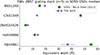 |
Fig. 3. Comparison of emission-line EWs in the JWST grating stack for the z > 5 sample (purple) with median values from the SDSS quasar catalog of Wu & Shen (2022) (green). Circles and squares represent measured lines with 1σ uncertainties, while left-pointing arrows denote 3σ upper limits for undetected lines in the JWST stack. Only the broad components are considered for C IV, He II, and Hβ. In most cases, error bars are smaller than the marker symbols and are not visually apparent. |
These results highlight a systematic difference in the ionizing spectra and BLR conditions of high-redshift AGNs compared to their lower redshift analogs. The weakness or absence of high-ionization lines (CIV, HeII, [NeV]) – relative to the robust Balmer and [OIII] emission – places strong constraints on the shape of the ionizing SED and the BLR geometry. As we discuss below, such trends may favor either (1) soft, filtered continua due to radiative-transfer effects or shielding in the inner disk; or (2) super-Eddington accretion scenarios in which the ionizing output is intrinsically anisotropic and collimated, illuminating only portions of the BLR.
4. Accretion flow diagnostics at z > 5 from BLR emission
The extreme distances and early cosmic epochs probed by z > 5 JWST-selected AGNs offer a unique opportunity to test whether broad-line diagnostics – developed primarily for low-redshift AGNs or bright QSOs – can still constrain the physical nature of accretion flows in the low-metallicity, rapidly evolving environments of the early Universe. To model the emission-line response to different accretion scenarios, we used a spectral synthesis code. Calculations were performed with version 23.01 of CLOUDY (Chatzikos et al. 2023; Gunasekera et al. 2023). It self-consistently computes the thermal, ionization, and emission-line structure of gas exposed to an AGN continuum.
In this work, we focused on sub-Eddington models for the AGN SED, specifically in the context of their ionizing continua. Two representative families of SEDs are considered, whose spectral shapes are compared in Figure 4. These are the following:
-
The empirical SED model of Jin et al. (2012), constructed from a statistically significant sample of local, unobscured Type 1 AGNs observed with both XMM-Newton and SDSS. This model captures the average broadband emission properties across the optical, UV, and X-ray regimes, and incorporates contributions from the accretion disk, soft excess, and hot corona. Its data-driven nature makes it especially suitable for anchoring the ionizing output of AGNs in the nearby Universe under moderate accretion conditions.
-
The theoretical framework developed by Pezzulli et al. (2017), which combines a thin accretion disk with a Comptonizing corona to self-consistently model the SED as a function of the black-hole mass and accretion rate. Designed to probe the growth of early SMBHs, this model is tailored for high-redshift AGNs, offering predictions for how the shape and hardness of the ionizing spectrum evolve with redshift and fueling conditions. While the model formally includes photon trapping, this effect only becomes important near the Eddington limit; for sub-Eddington accretion rates, photon trapping is negligible, and the emergent SED reflects the intrinsic disk-corona emission.
Both SED families were selected to represent sub-Eddington accretion regimes around moderate-mass black holes, with Eddington ratios of L/LEdd ≲ 0.1 and typical black-hole masses of 107–108 M⊙; these are consistent with expectations for radiatively efficient but moderately accreting AGNs (see also the discussion of a low L/Ledd SED in Ferland et al. 2020) and consistent with the average black-hole mass of our sample, ⟨MBH⟩≃107.2 M⊙. While single-epoch black-hole mass estimates at high redshift might be subject to systematic uncertainties (see, e.g., Rusakov et al. (2025), Greene et al. (2026); but see also, e.g., Juodžbalis et al. (2025b) for evidence supporting the locally calibrated single-epoch method), we verified that adopting an AGN SED with a lower black-hole mass (in our test the Pezzulli et al. (2017) SED with (MBH = 106 M⊙, i.e., assuming the black-hole masses were overestimated by 1–2 dex; e.g., Greene et al. 2026) does not change our conclusions. Indeed, as noted by Abuter et al. (2024), single-epoch virial estimators may overestimate black-hole masses, but this bias is minimized when using Hα, for which the error is comparable to the intrinsic scatter of the scaling relation. Also, as recently shown by Juodžbalis et al. (2025b) for a JWST-selected AGN at z = 7, the black-hole mass independently measured through kinematics is consistent with the single-epoch mass within a 1σ scatter. These templates provide essential input for modeling the ionizing photon budgets and radiative feedback of AGNs during cosmic reionization and structure formation.
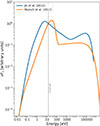 |
Fig. 4. νFν SEDs of Jin et al. (2012) and Pezzulli et al. (2017) families, normalized at 13.6 eV. The normalization energy is marked by the vertical dashed line; amplitudes are in arbitrary units and are used solely to compare spectral shapes. The Pezzulli et al. (2017) SED is harder near the hydrogen-ionization edge, leading to stronger excitation of high-ionization lines such as He II, whereas the Jin et al. (2012) SED exhibits a more prominent soft X-ray tail, contributing extra ionizing photons above the He II edge (54.4 eV). |
We constructed a grid of photoionization models tailored to conditions typical of the BLR (parameters are summarized in Table 1). All models assume constant-pressure conditions and a metallicity of 0.1 Z⊙, which is broadly consistent with what is inferred for these AGNs at z ≳ 5 (see Maiolino et al. 2024; Trefoloni et al. 2025). We adopted the solar reference from Grevesse et al. (2010) with variable He/H, C/O, and N/O according to the metallicity. Helium enrichment follows a primary-production from Dopita et al. (2000), and nitrogen and carbon follow a primary + secondary prescription from Groves et al. (2004). Dust and molecules were excluded, which is consistent with the BLR being within the sublimation radius. Each cloud was truncated at log(NH/cm−2) = 23, and models were terminated when the electron fraction fell below 10−2 or the temperature dropped below 4000 K. The hydrogen gas density was fixed at log (nH/cm−3) = 10, and the ionization parameter, i.e., the dimensionless ratio between the density of hydrogen-ionizing photons and the hydrogen number density, was varied across the log U = −3.5 to −1.0 range. The inclusion of low-ionization parameters (down to log U ≃ −3.5) allowed us to probe BLR conditions where the number of hydrogen-ionizing photons per particle is minimal.
Physical parameters adopted for the BLR photoionization CLOUDY models setup.
At fixed gas density, decreasing log U causes the zone of doubly ionized helium (HeIII) and other high-ionization regions to contract, thereby reducing the luminosity of recombination lines such as HeII λ4686 and high-ionization collisionally excited lines such as CIV λ1549. In contrast, low-ionization lines (e.g., Hβ) remain less affected or may even increase in relative strength. If the observed weakness of high-ionization features is primarily driven by a low-ionization parameter, models with log U ≲ −3 should reproduce the observed Hβ/HeII λ4686 broad-line ratios. Failure to reproduce these ratios at low log U would instead support alternative explanations.
In parallel, we compared the EWs of Hβ, HeII λ4686, and CIV λ1549 predicted by the models to those observed. In CLOUDY, EWs were computed by integrating the emergent line flux and referencing it to the transmitted continuum at the line wavelength. To isolate geometric effects, we ran models across a range of BLR covering factors (CFs). If the observed EWs of all broad emission lines are reproduced by a common CF envelope, the variations can be attributed to a non-unity CF rather than intrinsic differences in the ionizing continuum. Conversely, if the observed values require different CFs for different lines, or lie outside the model envelope altogether, then a purely geometric interpretation is insufficient. This would instead point to intrinsic shortcomings in the assumed SEDs, ionization structure, or BLR physics. For upper and lower limits, we consider models to be consistent if their CF envelope intersects the region allowed by the observations. A persistent mismatch across the full ionization grid would favor scenarios involving a soft or filtered SED, or super-Eddington accretion.
Figures 5–8 compare the model predictions from the two sub-Eddington SED templates against four key spectroscopic diagnostics in the z > 5 stack:
-
Hβ EW (Fig. 5). The observed Hβ EW of ∼37 Å is matched only by the Jin et al. (2012) soft SED, and only within a narrow region at low ionization (log U ≲ −3) and a low CF (CF ≲0.2). For a higher log U, the predicted EW exceeds the observed value unless the CF is reduced to unrealistically low levels. The Pezzulli et al. (2017) SED fails to reproduce the observed Hβ strength at any log U or CF combination, consistently overpredicting the line flux even at minimal covering. These constraints strongly disfavor harder SEDs and point to the need for both soft ionizing spectra and small BLR covering factors.
-
HeII λ4686 EW (Fig. 6). The 3σ upper limit on the broad HeII EW (∼13 Å) rules out the Pezzulli et al. (2017) SED for models with CFs ≳0.2, where it predicts HeII strengths exceeding 15 Å. The Jin et al. (2012) model, with a softer ionizing continuum, yields substantially lower HeII EWs and remains consistent with the observational upper limit across the entire log U–CF space (except for the highest CFs at log U ≳ −3). These results disfavor hard, unfiltered SEDs unless the BLR is shielded from high-energy photons, such as in geometries with inner absorption or anisotropic emission.
-
Hβ/HeII λ4686 ratio (Fig. 7). The observed lower limit on the broad Hβ/HeII ratio (> 2.7) is met by both models across the entire log U space. While this diagnostic does not strongly distinguish between the two SEDs, it supports the same region in log U–CF space favored by the individual-line EWs.
-
CIV λ1549 EW (Fig. 8). The 3σ upper limit of ∼13 Å on the CIV EW provides stringent constraints. Both the Pezzulli et al. (2017) and Jin et al. (2012) SEDs overpredict CIV emission at log U ≳ −2.5 – −2 and CF ≳0.4, and they are therefore strongly disfavored in that regime.
Together, these four diagnostics favor a model with a soft ionizing continuum (e.g., Jin et al. 2012), moderate ionization parameter (log U ∼ −2.5), and a covering factor of ∼0.1–0.5. Harder SEDs, such as Pezzulli et al. (2017), are incompatible with the combined observational constraints unless implausibly low BLR covering factors are invoked.
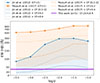 |
Fig. 5. Broad Hβ EWs as function of ionization parameter log U, derived from sub-Eddington CLOUDY models (parameters listed in Table 1). Different line styles indicate varying broad-line-region CFs, ranging from 1.0 to 0.1; models with the same SED share the same color. The shaded region for each SED represents the envelope spanned by CF values from 1.0 down to 0.1. The horizontal dark violet line marks the observed EW of broad Hβ measured in the z > 5 grating stack. The vertical axis uses a symlog scale (linear below 200 Å, logarithmic above). |
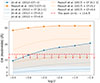 |
Fig. 6. Broad HeII λ4686 EWs as function of ionization parameter log U, derived from sub-Eddington CLOUDY models (parameters listed in Table 1). Different line styles indicate varying broad-line-region CFs, from 1.0 to 0.1; models with the same SED share the same color. The shaded region for each SED shows the envelope spanned by varying CF. The downward-pointing red arrows indicate the 3σ upper limit on the EW of broad HeII λ4686 measured in the z > 5 grating stack. The vertical axis uses a symlog scale (linear below 25 Å, logarithmic above). |
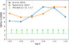 |
Fig. 7. Predicted ratio of broad Hβ to HeII λ4686 emission as function of ionization parameter log U, based on the sub-Eddington CLOUDY models listed in Table 1. Blue and orange curves correspond to the Jin et al. (2012) and Pezzulli et al. (2017) SEDs, respectively. As the ratio is independent of the covering factor, only one curve is shown per SED. The upward-pointing green arrow marks the 3σ lower limit on the broad-line Hβ/HeII ratio measured in the z > 5 grating stack. |
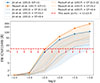 |
Fig. 8. Broad C IV λ1549 EWs versus ionization parameter log U from sub-Eddington CLOUDY models (parameters in Table 1). Line styles indicate different broad-line region CFs; colors distinguish SEDs. The downward-pointing red arrows mark the 3σ upper limit from the z > 5 grating stack. For consistency with our measurements, only the stronger CIV λ1549 component from CLOUDY is shown. The vertical axis uses a symlog scale (linear below 10 Å, logarithmic above). |
5. Summary and discussion
We have presented a spectroscopic analysis of 32 broad-line AGNs identified in JWST/NIRSpec observations from the JADES survey, spanning a redshift range of 1.7 < z < 9. The initial parent sample contained 34 objects, but two X-ray–detected AGNs were excluded from the present analysis. Emission-line diagnostics from both prism and grating stacks were used to characterize the ionizing spectra and physical conditions of the BLR, with particular focus on the high-redshift (z > 5) regime, where AGNs show puzzling deviations from standard photoionization expectations. While EWs for all redshift bins are listed in Table A.1, Figures 5–8 focus exclusively on the z > 5 stacks and their corresponding photoionization models. This work is primarily concerned with the high-redshift AGN population; the lower redshift stacks (z < 3.5, based on only five objects, and 3.5 < z < 5) are included mainly for completeness rather than detailed analysis. Moreover, these data are not constraining, and their inclusion in the plots would not yield any additional insight. A comparison between models and these lower-redshift bins is beyond the scope of this study. Consequently, our discussion and conclusions are restricted to the z > 5 sample, and EWs from the lower-redshift stacks are not used in any physical interpretation.
At z > 5, we find a suppression of high-ionization rest-frame UV lines such as HeII λ1640, CIV λ1549, and NV λ1240. These lines are either undetected or appear with extremely low EWs, while Balmer lines (Hα, Hβ) and low-ionization lines such as HeI λ5876 remain strong and well detected. Narrow forbidden lines such as [NeV] λ3426 (ionization potential ∼97 eV) and [NeIV] λ2424 (∼63 eV) are also weak or absent at high redshift, further supporting a soft ionizing photon field.
To interpret these trends, we constructed a suite of CLOUDY photoionization models using two sub-Eddington SEDs: the empirical template of Jin et al. (2012), representative of nearby AGNs with moderate Eddington ratios; and the theoretical disk-corona model of Pezzulli et al. (2017), designed for high-redshift black-hole growth. We varied the ionization parameter log U from −3.5 to −1.0 and explored a range of CFs between 0.1 and 1.0. All models assumed constant-pressure clouds with nH = 1010 cm−3 and Z = 0.1 Z⊙ and included realistic prescriptions for helium, nitrogen, and carbon enrichment. Dust and molecules were excluded.
Four key diagnostics were compared against the z > 5 observations: the EWs of Hβ, HeII λ4686, and CIV λ1549; and the Hβ/HeII λ4686 broad-line ratio. These constraints jointly delineate a narrow region of viable model space. 1) The observed Hβ EW (∼37 Å) is never matched by the Pezzulli et al. (2017) SED across the full log U and CF space. The Jin et al. (2012) SED reproduces the observed value only at very low ionization (log U ∼ −3) and low CFs (CF ∼0.1–0.3). This indicates a strong preference for soft ionizing continua and limited BLR coverage. 2) The 3σ upper limit on HeII (∼13 Å) excludes the Pezzulli et al. (2017) model at log U ≳ −2.5, where predicted EWs exceed 15 Å even at CF ≳0.2. The softer Jin et al. (2012) SED predicts significantly lower HeII emission and remains fully consistent with the observational limit across the full log U-CF parameter space. These results disfavor hard SEDs unless the BLR is substantially shielded from high-energy photons. 3) The observed lower limit on the broad Hβ/HeII ratio (> 2.7) is not a strong discriminator among SEDs and is satisfied by both models across the whole log U space. Finally, 4) the 3σ upper limit of ∼13 Å on the C IV EW provides a stringent constraint. Both the Pezzulli et al. (2017) and Jin et al. (2012) SEDs tend to overpredict C IV emission for log U ≳ −2 and CF ≳ 0.4, and they are therefore disfavored in that region of parameter space.
Taken together, these four diagnostics favor a model with a soft ionizing continuum (e.g., Jin et al. 2012), moderate-to-low ionization parameter (log U ∼ −2.5 to −3), and a CF of ∼0.1–0.5. Harder SEDs such as those of Pezzulli et al. (2017) are incompatible with the combined observational constraints unless implausibly low BLR covering factors are invoked. We verified that these conclusions are not sensitive to the adopted gas density. We performed additional tests using photoionization models with log (nH/cm−3) = 8 and 12. While varying nH shifts the absolute EW values and can slightly modify the preferred ionization parameter, log U, it does not resolve the key discrepancies between model predictions and observed data. Even within the preferred regime, some tension remains in simultaneously reproducing all observed EWs, highlighting possible limitations of static, sub-Eddington photoionization models. These discrepancies may motivate the need for alternative physical scenarios. One such possibility is the presence of a filtered or anisotropic ionizing continuum, as may occur in super-Eddington accretion flows. In this case, the far-UV and soft X-ray continuum can be shielded from the BLR by inner disk structures or collimated outflows, selectively suppressing high-ionization lines while leaving Balmer emission relatively unaffected. This interpretation is consistent with both the observed-line EWs and the known X-ray weakness of many high-z JWST AGNs.
Super-Eddington accretion flows are expected to yield emergent spectra that differ markedly from the standard thin-disk paradigm. Recent calculations by Madau (2025) model the radiative output of such flows, incorporating the effects of radiation pressure and funnel-like geometries. In this framework, the inner disk inflates to form an optically thick funnel along the rotation axis, collimating ionizing photons toward polar directions. Equatorial sightlines are dominated by reprocessed emission, resulting in highly anisotropic SEDs: the escaping radiation becomes significantly harder and more luminous at low inclination angles, while the extreme UV and soft X-ray output is strongly suppressed for θ ≳ 60°. This anisotropy has important consequences for emission-line diagnostics. The angular dependence of the ionizing continuum leads to a reduced production of HeII-ionizing photons at large viewing angles, even though the hydrogen-ionizing luminosity remains high when averaged over a solid angle. Such directionally filtered SEDs may provide a compelling explanation for the observed combination of strong Balmer lines and weak, high-ionization emission in many JWST-selected broad-line AGNs. Detailed implications for BLR line ratios and covering factors will be explored in a companion paper.
An alternative explanation for the observed suppression of high-ionization lines in JWST AGNs invokes obscuration or filtering of the ionizing continuum by intervening material. Tang et al. (2025) suggest that the absence of lines such as HeII and CIV in many high-redshift sources may be due to attenuation by dense neutral gas and dust, which absorb the EUV and soft X-ray photons required to excite these transitions. Similarly, Ishibashi et al. (2025) propose that X-ray weakness arises from radiative feedback and obscuration by dust-poor, high-column-density gas, which can absorb high-energy photons while allowing lower-energy emission (e.g., Balmer lines) to escape. These scenarios imply that the BLR may not be illuminated uniformly, and that anisotropic or filtered radiation fields – rather than intrinsically soft SEDs or extreme accretion physics – could account for the observed spectroscopic trends. Future constraints on the geometry, composition, and ionization state of the absorbing medium will be key to distinguishing between these possibilities.
Our photoionization analysis assumes that the observed EWs directly reflect the underlying ionizing SED, with no differential dust extinction between the BLR and the continuum source. If the dust acts as a uniform screen at large distances, EWs remain unchanged and our CLOUDY modeling remains valid. However, the observed Balmer decrements (Hα/Hβ > 10) suggest significant reddening (see Table A.1 and Brooks et al. 2025), which could imply non-negligible, wavelength-dependent attenuation. If dust is patchy or mixed within the BLR, or if it affects line and continuum emission differently, then our assumptions may break down. Alternatively, the large broad-line Balmer decrement could be a result of strong collisional excitation in the BLR, as observed and suggested for some lower redshift AGNs (Ilić et al. 2012), or a radiative-transfer effect when Balmer lines become optically thick (Chang et al. 2026; Ji et al. 2026). We will explore alternative BLR models to investigate the above scenarios in future work.
Acknowledgments
XJ and RM acknowledge ERC Advanced Grant 695671 “QUENCH” and support by the Science and Technology Facilities Council (STFC) and by the UKRI Frontier Research grant RISEandFALL. This work is based on observations made with the NASA/ESA/CSA James Webb Space Telescope. The data are available at the Mikulski Archive for Space Telescopes (MAST) at the Space Telescope Science Institute, which is operated by the Association of Universities for Research in Astronomy, Inc., under NASA contract NAS 5-03127 for JWST. The reduced spectra used in this work are from the public data release of the JADES survey, available at https://jades-survey.github.io/scientists/data.html.
References
- Abuter, R., Allouche, F., Amorim, A., et al. 2024, Nature, 627, 281 [NASA ADS] [CrossRef] [Google Scholar]
- Ananna, T. T., Bogdán, Á., Kovács, O. E., Natarajan, P., & Hickox, R. C. 2024, ApJ, 969, L18 [NASA ADS] [CrossRef] [Google Scholar]
- Berg, D. A., Chisholm, J., Erb, D. K., et al. 2021, ApJ, 922, 170 [CrossRef] [Google Scholar]
- Bertemes, C., Wylezalek, D., Rupke, D. S. N., et al. 2025, A&A, 693, A176 [NASA ADS] [CrossRef] [EDP Sciences] [Google Scholar]
- Boroson, T. A., & Green, R. F. 1992, ApJS, 80, 109 [Google Scholar]
- Brazzini, M., D’Eugenio, F., Maiolino, R., et al. 2025, MNRAS, 544, L167 [Google Scholar]
- Brooks, M., Simons, R. C., Trump, J. R., et al. 2025, ApJ, 986, 177 [Google Scholar]
- Bunker, A. J., Cameron, A. J., Curtis-Lake, E., et al. 2024, A&A, 690, A288 [NASA ADS] [CrossRef] [EDP Sciences] [Google Scholar]
- Capellupo, D. M., Netzer, H., Lira, P., Trakhtenbrot, B., & Mejía-Restrepo, J. 2015, MNRAS, 446, 3427 [NASA ADS] [CrossRef] [Google Scholar]
- Cappellari, M. 2017, MNRAS, 466, 798 [Google Scholar]
- Cappellari, M. 2023, MNRAS, 526, 3273 [NASA ADS] [CrossRef] [Google Scholar]
- Cappellari, M., & Emsellem, E. 2004, PASP, 116, 138 [Google Scholar]
- Carnall, A. C. 2017, ArXiv e-prints [arXiv:1705.05165] [Google Scholar]
- Carniani, S., Venturi, G., Parlanti, E., et al. 2024, A&A, 685, A99 [NASA ADS] [CrossRef] [EDP Sciences] [Google Scholar]
- Chang, S.-J., Gronke, M., Matthee, J., & Mason, C. 2026, MNRAS, 545, staf2131 [Google Scholar]
- Chatzikos, M., Bianchi, S., Camilloni, F., et al. 2023, Rev. Mex. Astron. Astrofis., 59, 327 [Google Scholar]
- Cleri, N. J., Olivier, G. M., Hutchison, T. A., et al. 2023a, ApJ, 953, 10 [NASA ADS] [CrossRef] [Google Scholar]
- Cleri, N. J., Yang, G., Papovich, C., et al. 2023b, ApJ, 948, 112 [NASA ADS] [CrossRef] [Google Scholar]
- Cleri, N. J., Olivier, G. M., Backhaus, B. E., et al. 2025, ApJ, 994, 146 [Google Scholar]
- Coatman, L., Hewett, P. C., Banerji, M., & Richards, G. T. 2016, MNRAS, 461, 647 [NASA ADS] [CrossRef] [Google Scholar]
- Cohn, J. H., Durodola, E., Casey, Q. O., Lambrides, E., & Hickox, R. C. 2025, ApJ, 988, L61 [Google Scholar]
- Dasyra, K. M., Ho, L. C., Netzer, H., et al. 2011, ApJ, 740, 94 [NASA ADS] [CrossRef] [Google Scholar]
- De Graaff, A., Rix, H.-W., Carniani, S., et al. 2024, A&A, 684, A87 [NASA ADS] [CrossRef] [EDP Sciences] [Google Scholar]
- de Graaff, A., Rix, H.-W., Naidu, R. P., et al. 2025, A&A, 701, A168 [NASA ADS] [CrossRef] [EDP Sciences] [Google Scholar]
- De Graaff, A., Setton, D. J., Brammer, G., et al. 2025, Nat. Astron., 9, 280 [Google Scholar]
- D’Eugenio, F., Cameron, A. J., Scholtz, J., et al. 2025a, ApJS, 277, 4 [Google Scholar]
- D’Eugenio, F., Maiolino, R., Perna, M., et al. 2025b, MNRAS, submitted [arXiv:2503.11752] [Google Scholar]
- D’Eugenio, F., Nelson, E., Ji, X., et al. 2025c, ApJ, submitted [arXiv:2510.00101] [Google Scholar]
- D’Eugenio, F., Juodžbalis, I., Ji, X., et al. 2026, MNRAS, 545, staf2117 [Google Scholar]
- Done, C., Davis, S. W., Jin, C., Blaes, O., & Ward, M. 2012, MNRAS, 420, 1848 [Google Scholar]
- Dopita, M. A., Kewley, L. J., Heisler, C. A., & Sutherland, R. S. 2000, ApJ, 542, 224 [NASA ADS] [CrossRef] [Google Scholar]
- Eisenstein, D. J., Willott, C., Alberts, S., et al. 2023, ArXiv e-prints [arXiv:2306.02465] [Google Scholar]
- Feltre, A., Charlot, S., & Gutkin, J. 2016, MNRAS, 456, 3354 [Google Scholar]
- Ferland, G. J., Done, C., Jin, C., Landt, H., & Ward, M. J. 2020, MNRAS, 494, 5917 [Google Scholar]
- Geris, S., Maiolino, R., Isobe, Y., et al. 2026, MNRAS, 545, staf1979 [Google Scholar]
- Greene, J. E., Setton, D. J., Furtak, L. J., et al. 2026, ApJ, 996, 129 [Google Scholar]
- Grevesse, N., Asplund, M., Sauval, A. J., & Scott, P. 2010, Ap&SS, 328, 179 [Google Scholar]
- Groves, B. A., Dopita, M. A., & Sutherland, R. S. 2004, ApJS, 153, 75 [NASA ADS] [CrossRef] [Google Scholar]
- Gunasekera, C. M., van Hoof, P. A. M., Chatzikos, M., & Ferland, G. J. 2023, Res. Notes Am. Astron. Soc., 7, 246 [Google Scholar]
- Hall, P. B., Sarrouh, G. T., & Horne, K. 2018, ApJ, 854, 93 [Google Scholar]
- Harikane, Y., Zhang, Y., Nakajima, K., et al. 2023, ApJ, 959, 39 [NASA ADS] [CrossRef] [Google Scholar]
- Ilić, D., Popović, L. Č., La Mura, G., Ciroi, S., & Rafanelli, P. 2012, A&A, 543, A142 [NASA ADS] [CrossRef] [EDP Sciences] [Google Scholar]
- Inayoshi, K., & Maiolino, R. 2025, ApJ, 980, L27 [Google Scholar]
- Ishibashi, W., Fabian, A. C., Maiolino, R., Gursahani, Y., & Reynolds, C. S. 2025, MNRAS, 544, 726 [Google Scholar]
- Isobe, Y., Maiolino, R., D’Eugenio, F., et al. 2025, MNRAS, 541, L71 [Google Scholar]
- Izotov, Y. I., Thuan, T. X., & Privon, G. 2012, MNRAS, 427, 1229 [NASA ADS] [CrossRef] [Google Scholar]
- Izotov, Y. I., Thuan, T. X., & Guseva, N. G. 2021, MNRAS, 508, 2556 [NASA ADS] [CrossRef] [Google Scholar]
- Ji, X., Maiolino, R., Übler, H., et al. 2025, MNRAS, 544, 3900 [Google Scholar]
- Ji, X., D’Eugenio, F., Juodžbalis, I., et al. 2026, MNRAS, 545, staf2235 [Google Scholar]
- Jin, C., Ward, M., Done, C., & Gelbord, J. 2012, MNRAS, 420, 1825 [Google Scholar]
- Juodžbalis, I., Ji, X., Maiolino, R., et al. 2024, MNRAS, 535, 853 [CrossRef] [Google Scholar]
- Juodžbalis, I., Maiolino, R., Baker, W. M., et al. 2025a, MNRAS, submitted [arXiv:2504.03551] [Google Scholar]
- Juodžbalis, I., Marconcini, C., D’Eugenio, F., et al. 2025b, ArXiv e-prints [arXiv:2508.21748] [Google Scholar]
- Katz, H., Kimm, T., Ellis, R. S., Devriendt, J., & Slyz, A. 2023, MNRAS, 524, 351 [CrossRef] [Google Scholar]
- Kocevski, D. D., Onoue, M., Inayoshi, K., et al. 2023, ApJ, 954, L4 [NASA ADS] [CrossRef] [Google Scholar]
- Kocevski, D. D., Finkelstein, S. L., Barro, G., et al. 2025, ApJ, 986, 126 [Google Scholar]
- Kokubo, M., & Harikane, Y. 2025, ApJ, 995, 24 [Google Scholar]
- Kollatschny, W., & Zetzl, M. 2013, A&A, 549, A100 [NASA ADS] [CrossRef] [EDP Sciences] [Google Scholar]
- Kubota, A., & Done, C. 2019, MNRAS, 489, 524 [NASA ADS] [CrossRef] [Google Scholar]
- Lambrides, E., Garofali, K., Larson, R., et al. 2024, ArXiv e-prints [arXiv:2409.13047] [Google Scholar]
- Laor, A. 2006, ApJ, 643, 112 [Google Scholar]
- Lupi, A., Trinca, A., Volonteri, M., Dotti, M., & Mazzucchelli, C. 2024, A&A, 689, A128 [NASA ADS] [CrossRef] [EDP Sciences] [Google Scholar]
- Luridiana, V., Morisset, C., & Shaw, R. A. 2015, A&A, 573, A42 [NASA ADS] [CrossRef] [EDP Sciences] [Google Scholar]
- Madau, P. 2025, ApJ, submitted [arXiv:2501.09854] [Google Scholar]
- Madau, P., & Haardt, F. 2024, ApJ, 976, L24 [Google Scholar]
- Maiolino, R., Scholtz, J., Curtis-Lake, E., et al. 2024, A&A, 691, A145 [NASA ADS] [CrossRef] [EDP Sciences] [Google Scholar]
- Maiolino, R., Risaliti, G., Signorini, M., et al. 2025, MNRAS, 538, 1921 [Google Scholar]
- Marconcini, C., D’Eugenio, F., Maiolino, R., et al. 2025, A&A, 699, A154 [NASA ADS] [CrossRef] [EDP Sciences] [Google Scholar]
- Marziani, P., Sulentic, J. W., Negrete, C. A., et al. 2010, MNRAS, 409, 1033 [Google Scholar]
- Matthee, J., Naidu, R. P., Brammer, G., et al. 2024, ApJ, 963, 129 [NASA ADS] [CrossRef] [Google Scholar]
- Naidu, R. P., Matthee, J., Katz, H., et al. 2025, ArXiv e-prints [arXiv:2503.16596] [Google Scholar]
- Nanayakkara, T., Brinchmann, J., Boogaard, L., et al. 2019, A&A, 624, A89 [NASA ADS] [CrossRef] [EDP Sciences] [Google Scholar]
- Negus, J., Comerford, J. M., Sánchez, F. M., et al. 2023, ApJ, 945, 127 [NASA ADS] [CrossRef] [Google Scholar]
- Olivier, G. M., Berg, D. A., Chisholm, J., et al. 2022, ApJ, 938, 16 [NASA ADS] [CrossRef] [Google Scholar]
- Osterbrock, D. E., & Ferland, G. J. 2006, Astrophysics of Gaseous Nebulae and Active Galactic Nuclei [Google Scholar]
- Pacucci, F., & Narayan, R. 2024, ApJ, 976, 96 [NASA ADS] [CrossRef] [Google Scholar]
- Pezzulli, E., Valiante, R., Orofino, M. C., et al. 2017, MNRAS, 466, 2131 [NASA ADS] [CrossRef] [Google Scholar]
- Reines, A. E., & Volonteri, M. 2015, ApJ, 813, 82 [NASA ADS] [CrossRef] [Google Scholar]
- Richards, G. T., Kruczek, N. E., Gallagher, S. C., et al. 2011, AJ, 141, 167 [Google Scholar]
- Richardson, C. T., Wels, J., Garofali, K., et al. 2025, ApJ, 993, 154 [Google Scholar]
- Rieke, M. J., Robertson, B., Tacchella, S., et al. 2023, ApJS, 269, 16 [NASA ADS] [CrossRef] [Google Scholar]
- Rusakov, V., Watson, D., Nikopoulos, G. P., et al. 2025, Nature, submitted [arXiv:2503.16595] [Google Scholar]
- Sacchi, A., & Bogdán, Á. 2025, ApJ, 989, L30 [Google Scholar]
- Saxena, A., Pentericci, L., Mirabelli, M., et al. 2020, A&A, 636, A47 [NASA ADS] [CrossRef] [EDP Sciences] [Google Scholar]
- Scholtz, J., Maiolino, R., D’Eugenio, F., et al. 2025, A&A, 697, A175 [NASA ADS] [CrossRef] [EDP Sciences] [Google Scholar]
- Shirazi, M., & Brinchmann, J. 2012, MNRAS, 421, 1043 [NASA ADS] [CrossRef] [Google Scholar]
- Spoon, H. W. W., & Holt, J. 2009, ApJ, 702, L42 [NASA ADS] [CrossRef] [Google Scholar]
- Tang, M., Stark, D. P., Plat, A., et al. 2025, ApJ, 991, 217 [Google Scholar]
- Taylor, A. J., Kokorev, V., Kocevski, D. D., et al. 2025, ApJ, 989, L7 [Google Scholar]
- Thuan, T. X., & Izotov, Y. I. 2005, ApJS, 161, 240 [NASA ADS] [CrossRef] [Google Scholar]
- Trefoloni, B., Ji, X., Maiolino, R., et al. 2025, A&A, 700, A203 [NASA ADS] [CrossRef] [EDP Sciences] [Google Scholar]
- Treiber, H., Greene, J. E., Weaver, J. R., et al. 2025, ApJ, 984, 93 [Google Scholar]
- Übler, H., Maiolino, R., Curtis-Lake, E., et al. 2023, A&A, 677, A147 [Google Scholar]
- Vanden Berk, D. E., Richards, G. T., Bauer, A., et al. 2001, AJ, 122, 549 [Google Scholar]
- Vazdekis, A., Koleva, M., Ricciardelli, E., Röck, B., & Falcón-Barroso, J. 2016, MNRAS, 463, 3409 [Google Scholar]
- Wang, J.-M., Qiu, J., Du, P., & Ho, L. C. 2014, ApJ, 797, 65 [NASA ADS] [CrossRef] [Google Scholar]
- Wang, B., Leja, J., Katz, H., et al. 2025, ApJ, submitted [arXiv:2508.18358] [Google Scholar]
- Wu, Q., & Shen, Y. 2022, ApJS, 263, 42 [NASA ADS] [CrossRef] [Google Scholar]
- Yue, M., Eilers, A.-C., Ananna, T. T., et al. 2024, ApJ, 974, L26 [CrossRef] [Google Scholar]
The fixed ratios were applied to the [OIII] λλ4959,5007, [NII] λλ6548,6583, [NeV] λλ3346,3426, [NeIII] λλ3869,3968, CIV λλ1548,1551, NV λλ1238,1242, and MgII λλ2796,2803 doublets, with the fluxes of the fainter lines scaled from the brightest component in each pair.
Appendix A: Equivalent width table
Rest-frame equivalent widths (in Å) of prominent emission lines measured in stacked JWST/NIRSpec spectra of Type 1 AGNs.
Appendix B: Stack spectra
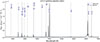 |
Fig. B.1. Stack of the rest-frame (G140M+G235M+G395M) grating spectra in the low-redshift bin (z < 3.5). The black line represents the best-fit from our pPXF fitting procedure, while the blue line shows the observed stacked spectrum. For visualization, the normalized stack was multiplied by the mean [OIII]λ5007 flux of the 5 contributing objects; this rescaling is used only for the figure and does not affect any measurements. |
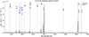 |
Fig. B.2. Stack of the rest-frame (G140M+G235M+G395M) grating spectra in the intermediate redshift bin (3.5 < z < 5). Color coding as figure above. For visualization purposes, the normalized stack has been multiplied by the mean [OIII]λ5007 flux of the 12 contributing objects. This rescaling affects only the plotted figure and not the underlying measurements. |
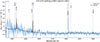 |
Fig. B.3. Stack of the rest-frame G140M grating spectra in the intermediate-redshift bin (3.5 < z < 5). Color coding as figures above. For visualization, the normalized stack was multiplied by the mean [OIII]λ5007 flux of the 11 contributing objects; this rescaling is used only for the figure and does not affect any measurements. The gray band masks a probable oversampling error, thus it has been removed from the fitting. |
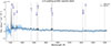 |
Fig. B.4. Stack of the rest-frame G140M grating spectra in the high-redshift bin (z > 5). Color coding as figures above. For visualization, the normalized stack was multiplied by the mean [OIII]λ5007 flux of the 14 contributing objects; this rescaling is used only for the figure and does not affect any measurements. |
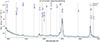 |
Fig. B.5. Stack of the rest-frame prism spectra in the low-redshift bin (z < 3.5). Color coding as figures above. For visualization purposes, the normalized stack has been multiplied by the mean [OIII]λ5007 flux of the 5 contributing objects. This rescaling affects only the plotted figure and not the underlying measurements. |
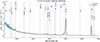 |
Fig. B.6. Stack of the rest-frame prism spectra in the intermediate-redshift bin (3.5 < z < 5). Color coding as figures above. For visualization purposes, the normalized stack has been multiplied by the mean [OIII]λ5007 flux of the 12 contributing objects. This rescaling affects only the plotted figure and not the underlying measurements. |
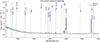 |
Fig. B.7. Stack of the rest-frame prism spectra in the high-redshift bin (z > 5). Color coding as figures above. For visualization purposes, the normalized stack has been multiplied by the mean [OIII]λ5007 flux of the 15 contributing objects. This rescaling affects only the plotted figure and not the underlying measurements. |
All Tables
Rest-frame equivalent widths (in Å) of prominent emission lines measured in stacked JWST/NIRSpec spectra of Type 1 AGNs.
All Figures
|
Fig. 1. Spectral wavelength coverage across dispersers for each object. Invalid or missing values are masked and shown as empty. The dashed vertical line at 3000 Å indicates a conventional division between the UV and optical regimes, though it is not used in the kinematic classification of emission lines. The treatment of lines near this boundary (e.g., [NeV] λ3426) is discussed in Section 3.2. |
| In the text | |
|
Fig. 2. Stack of JWST NIRSpec (G140M+G235M+G395M) grating spectra of JADES Type 1 AGNs in the high-redshift bin (z > 5). For visualization purposed, the normalized stack was multiplied by the mean [OIII] λ5007 flux of the 15 contributing objects; this rescaling is used only for the figure and not for any measurements. |
| In the text | |
|
Fig. 3. Comparison of emission-line EWs in the JWST grating stack for the z > 5 sample (purple) with median values from the SDSS quasar catalog of Wu & Shen (2022) (green). Circles and squares represent measured lines with 1σ uncertainties, while left-pointing arrows denote 3σ upper limits for undetected lines in the JWST stack. Only the broad components are considered for C IV, He II, and Hβ. In most cases, error bars are smaller than the marker symbols and are not visually apparent. |
| In the text | |
|
Fig. 4. νFν SEDs of Jin et al. (2012) and Pezzulli et al. (2017) families, normalized at 13.6 eV. The normalization energy is marked by the vertical dashed line; amplitudes are in arbitrary units and are used solely to compare spectral shapes. The Pezzulli et al. (2017) SED is harder near the hydrogen-ionization edge, leading to stronger excitation of high-ionization lines such as He II, whereas the Jin et al. (2012) SED exhibits a more prominent soft X-ray tail, contributing extra ionizing photons above the He II edge (54.4 eV). |
| In the text | |
|
Fig. 5. Broad Hβ EWs as function of ionization parameter log U, derived from sub-Eddington CLOUDY models (parameters listed in Table 1). Different line styles indicate varying broad-line-region CFs, ranging from 1.0 to 0.1; models with the same SED share the same color. The shaded region for each SED represents the envelope spanned by CF values from 1.0 down to 0.1. The horizontal dark violet line marks the observed EW of broad Hβ measured in the z > 5 grating stack. The vertical axis uses a symlog scale (linear below 200 Å, logarithmic above). |
| In the text | |
|
Fig. 6. Broad HeII λ4686 EWs as function of ionization parameter log U, derived from sub-Eddington CLOUDY models (parameters listed in Table 1). Different line styles indicate varying broad-line-region CFs, from 1.0 to 0.1; models with the same SED share the same color. The shaded region for each SED shows the envelope spanned by varying CF. The downward-pointing red arrows indicate the 3σ upper limit on the EW of broad HeII λ4686 measured in the z > 5 grating stack. The vertical axis uses a symlog scale (linear below 25 Å, logarithmic above). |
| In the text | |
|
Fig. 7. Predicted ratio of broad Hβ to HeII λ4686 emission as function of ionization parameter log U, based on the sub-Eddington CLOUDY models listed in Table 1. Blue and orange curves correspond to the Jin et al. (2012) and Pezzulli et al. (2017) SEDs, respectively. As the ratio is independent of the covering factor, only one curve is shown per SED. The upward-pointing green arrow marks the 3σ lower limit on the broad-line Hβ/HeII ratio measured in the z > 5 grating stack. |
| In the text | |
|
Fig. 8. Broad C IV λ1549 EWs versus ionization parameter log U from sub-Eddington CLOUDY models (parameters in Table 1). Line styles indicate different broad-line region CFs; colors distinguish SEDs. The downward-pointing red arrows mark the 3σ upper limit from the z > 5 grating stack. For consistency with our measurements, only the stronger CIV λ1549 component from CLOUDY is shown. The vertical axis uses a symlog scale (linear below 10 Å, logarithmic above). |
| In the text | |
|
Fig. B.1. Stack of the rest-frame (G140M+G235M+G395M) grating spectra in the low-redshift bin (z < 3.5). The black line represents the best-fit from our pPXF fitting procedure, while the blue line shows the observed stacked spectrum. For visualization, the normalized stack was multiplied by the mean [OIII]λ5007 flux of the 5 contributing objects; this rescaling is used only for the figure and does not affect any measurements. |
| In the text | |
|
Fig. B.2. Stack of the rest-frame (G140M+G235M+G395M) grating spectra in the intermediate redshift bin (3.5 < z < 5). Color coding as figure above. For visualization purposes, the normalized stack has been multiplied by the mean [OIII]λ5007 flux of the 12 contributing objects. This rescaling affects only the plotted figure and not the underlying measurements. |
| In the text | |
|
Fig. B.3. Stack of the rest-frame G140M grating spectra in the intermediate-redshift bin (3.5 < z < 5). Color coding as figures above. For visualization, the normalized stack was multiplied by the mean [OIII]λ5007 flux of the 11 contributing objects; this rescaling is used only for the figure and does not affect any measurements. The gray band masks a probable oversampling error, thus it has been removed from the fitting. |
| In the text | |
|
Fig. B.4. Stack of the rest-frame G140M grating spectra in the high-redshift bin (z > 5). Color coding as figures above. For visualization, the normalized stack was multiplied by the mean [OIII]λ5007 flux of the 14 contributing objects; this rescaling is used only for the figure and does not affect any measurements. |
| In the text | |
|
Fig. B.5. Stack of the rest-frame prism spectra in the low-redshift bin (z < 3.5). Color coding as figures above. For visualization purposes, the normalized stack has been multiplied by the mean [OIII]λ5007 flux of the 5 contributing objects. This rescaling affects only the plotted figure and not the underlying measurements. |
| In the text | |
|
Fig. B.6. Stack of the rest-frame prism spectra in the intermediate-redshift bin (3.5 < z < 5). Color coding as figures above. For visualization purposes, the normalized stack has been multiplied by the mean [OIII]λ5007 flux of the 12 contributing objects. This rescaling affects only the plotted figure and not the underlying measurements. |
| In the text | |
|
Fig. B.7. Stack of the rest-frame prism spectra in the high-redshift bin (z > 5). Color coding as figures above. For visualization purposes, the normalized stack has been multiplied by the mean [OIII]λ5007 flux of the 15 contributing objects. This rescaling affects only the plotted figure and not the underlying measurements. |
| In the text | |
Current usage metrics show cumulative count of Article Views (full-text article views including HTML views, PDF and ePub downloads, according to the available data) and Abstracts Views on Vision4Press platform.
Data correspond to usage on the plateform after 2015. The current usage metrics is available 48-96 hours after online publication and is updated daily on week days.
Initial download of the metrics may take a while.