| Issue |
A&A
Volume 707, March 2026
|
|
|---|---|---|
| Article Number | A251 | |
| Number of page(s) | 17 | |
| Section | Stellar atmospheres | |
| DOI | https://doi.org/10.1051/0004-6361/202557770 | |
| Published online | 17 March 2026 | |
A modeling perspective on the diversity of red supergiant stars exploding within circumstellar material
1
Institut d’Astrophysique de Paris, CNRS-Sorbonne Université,
98 bis boulevard Arago,
75014
Paris,
France
2
Cahill Center for Astrophysics, California Institute of Technology,
Pasadena,
CA
91125,
USA
★ Corresponding author: This email address is being protected from spambots. You need JavaScript enabled to view it.
Received:
20
October
2025
Accepted:
9
February
2026
Abstract
With the ever faster cadence of untargeted surveys of the sky, the supernova (SN) community will capture a growing number of shock breakouts in red supergiant (RSG) stars in the coming years. Expecting a high frequency of breakouts within circumstellar material (CSM), we have produced an extended regular and cubic grid of models covering low- to high-energy explosions, compact to extended CSM, and moderate- to high-density CSM. We document the main results from the radiation-hydrodynamics and nonlocal thermodynamic equilibrium radiative-transfer calculations over the first 15 d of evolution, including the bolometric and multiband light curves and the salient features from spectra. As before, CSM interaction is found to boost the UV brightness and shorten the optical rise time if compact. Higher ionization (e.g., as seen with O VI 3820 Å) is obtained for more compact CSM, and is maximum for explosions in a vacuum. CSM interaction also diversifies the spectral evolution as seen in line profile morphology, with electron-scattering broadening dominating during the IIn phase. In the absence of CSM, Doppler broadening dominates immediately after shock breakout and leads to strongly blueshifted emission in lines such as He II 4685.70 Å or C IV 5804.86 Å. This treasury of models will be used to analyze and predict future observations of RSG shock breakouts in CSM.
Key words: line: formation / radiative transfer / stars: mass-loss / supernovae: general
NASA Hubble Fellow
© The Authors 2026
 Open Access article, published by EDP Sciences, under the terms of the Creative Commons Attribution License (https://creativecommons.org/licenses/by/4.0), which permits unrestricted use, distribution, and reproduction in any medium, provided the original work is properly cited.
This article is published in open access under the Subscribe to Open model. This email address is being protected from spambots. You need JavaScript enabled to view it. to support open access publication.
1 Introduction
In recent years, high-cadence optical surveys of the sky have enabled us to routinely discover red supergiant (RSG) star explosions closer to shock breakout than ever before (see, e.g., Gal-Yam et al. 2011). Prompt photometric and spectroscopic follow-up have revealed the heterogeneity of these early-time properties. They include a range in UV brightness as captured by Swift (Irani et al. 2024; Jacobson-Galán et al. 2024b). They also include the frequent detection of events with spectral lines that instead of being Doppler broadened (as expected for emission from a fast-expanding photosphere), show a narrow core and extended, symmetric, electron-scattering broadened wings (e.g., Yaron et al. 2017; Zhang et al. 2020; Terreran et al. 2022; Jacobson-Galán et al. 2022). These spectral signatures were observed in hydrogen-rich (also known as Type II) core-collapse supernovae (SNe) as early as the 1980s (see, e.g., Niemela et al. 1985) and led to the creation of the new Type IIn class (Schlegel 1990). SN 1998S has become the prototype for this class because of its extraordinary luminosity, but also because of its unprecedented dataset that includes both low-resolution and high-resolution spectra, spectropolarimetry, and early- to late-time observations (e.g., Fassia et al. 2000, 2001; Leonard et al. 2000; Shivvers et al. 2015).
The general consensus is that these IIn signatures indicate the presence of circumstellar material (CSM) immediately at the surface of the exploding star, which causes the spectroscopic anomaly (Chugai 2001; Dessart et al. 2009; Groh 2014; Dessart et al. 2017; Boian & Groh 2020), but is also at the origin of a bolometric boost affecting the light curve for days or weeks (Moriya et al. 2011; Dessart et al. 2015; Morozova et al. 2017). More recent observations covering the earliest times immediately after the shock emergence at the progenitor surface suggest that the IIn signatures persist over different durations and with ionization properties that span from high values with SN 2013fs (e.g., lines of OVI) to low values with SN 1998S (e.g., lines of N III). A compendium of these events is presented in Jacobson-Galán et al. (2024b). Today, observations indicate that a significant fraction (i.e., several dozen percent) of Type II SNe are enshrouded in some CSM (Bruch et al. 2021, 2023), which warrants further study of the origin and implications of this material.
The nature of this material remains unclear today. It might arise from intense mass loss in the final years prior to core collapse, perhaps from core-rooted instabilities (Shiode & Quataert 2014; Fuller 2017) or mass exchange in interacting binaries (e.g., Ercolino et al. 2024). When the CSM is compact and directly present at the surface of the RSG progenitor, however, the material might simply correspond to the fundamental structure of RSG atmospheres, which are characterized by a sizable mass content and finite extent (Dessart et al. 2017; Soker 2021; Fuller & Tsuna 2024), perhaps affected by pulsational mass loss (e.g., Yoon & Cantiello 2010). One- and three-dimensional hydrodynamical simulations of RSG star envelopes have indeed revealed a complex structure and numerous instabilities that are not typically produced by standard stellar evolution calculations (see, e.g., Goldberg et al. 2022a; Ma et al. 2024, 2025; Bronner et al. 2025).
We extend our previous explorations (Dessart et al. 2017; Dessart & Jacobson-Galán 2023) to produce a cubic grid that regularly samples ejecta kinetic energy, CSM density, and CSM extent. By adopting a single progenitor (i.e., a solar metallicity 15 M⊙ star), we no doubt fall short of the probable diversity in SNe II exploding in CSM, in particular, because we miss partially stripped RSG progenitors. As is apparent from the results, however, this regular grid captures the properties not only of most of the events that have been observed, but also makes predictions beyond the current frontiers for what may be to come with future observations, in particular, with the strategically scheduled survey between the Vera Rubin Large Synoptic Survey Telescope and the Zwicky Transient Factory (Kasliwal et al. 2025). This grid of models will also be used to create a library of UV light curves and spectra (Dessart et al., in prep.) in anticipation of the hoped-for future observations with the Ultraviolet Transient Astronomy Satellite (i.e., ULTRASAT; Shvartzvald et al. 2024) and the Ultraviolet Explorer (i.e., UVEX; Kulkarni et al. 2021).
In the next section, we present the numerical setup for the calculations, including the choice of progenitor model, the simulations of the explosion until shock breakout, the radiation-hydrodynamics calculations of the shock breakout phase out to 15 d, and the postprocessing of these results at multiple epochs with radiative transfer. We then present the results from the radiation-hydrodynamics calculations in Sect. 3. We discuss the results for the multiband light curves in Sect. 4. Section 5 then discusses the properties of the model spectra, in particular, how Hα can be used as a probe of the evolving dynamical properties (Sect. 5.1), the wide range in ionization properties inferred from the spectra (Sect. 5.2), and the distinct signatures between the CSM and No-CSM cases (Sect. 5.3). We present our conclusions in Sect. 6.
2 Numerical setup
We performed radiation-hydrodynamics calculations with the code HERACLES (González et al. 2007; Vaytet et al. 2011; Dessart et al. 2015) for a variety of configurations corresponding to Type II SN ejecta interacting with the CSM. For each configuration, we postprocessed snapshots with the nonlocal thermodynamic equilibrium (NLTE) radiative transfer code CMFGEN (Hillier & Dessart 2012) using the Sobolev nonmonotonic solver (Dessart et al. 2015). The main asset in this approach is that the complex temperature, density, and (nonmonotonic) velocity structure of the interaction is retained, with the disadvantage of a nonopti-mal treatment of the radiative transfer (e.g., a more simplistic treatment of lines and the coupling between gas and radiation; see, e.g., the comparison in Dessart et al. 2025). This limitation means that the strength of some lines is uncertain (e.g., the emission blueward of He II 4685.70 Å due to C III 4647.42 Å and N III 4640.64 Å tends to be underestimated by the nonmonotonic solver relative to observations), and thus, more weight is given in this work on the line profile morphology and the relative strength between lines (e.g., to be used as an ionization diagnostic).
The goal of this study is thus to document the evolution of the gas and radiation over time (i.e., light curves and spectra) by starting at the time when the shock crosses the progenitor surface radius R∗. We thus cover in detail the rise to peak luminosity, the peak phase, and the subsequent decline until the interaction is over or until 15 d of physical time, whichever comes first. We limited the study to the cases of relatively short-lived interactions rather than enduring interactions lasting many weeks or months and producing bona fide Type IIn SNe. However, we mapped the parameter space more systematically than in our previous work, in particular, by considering explosions that produce a lower and higher ejecta kinetic energy than the canonical 1.2 × 1051 erg. The overall approach is identical to that presented in Dessart et al. (2017) and more recently in Dessart & Jacobson-Galán (2023), to which we refer for additional details. To avoid redundancy, we thus only describe what distinguishes the present simulations from these previous studies, namely the initial conditions for the progenitor and the explosion, and the numerical setup for the HERACLES and the CMFGEN simulations.
The current simulations are based on a grid of massive-star models evolved with MESA (Paxton et al. 2011, 2013, 2015) as part of a separate project studying dependences of preSN and SN properties on metallicity (the MESA simulations were performed in 2020 with version 10108). The original grid includes masses 12, 15, 20, and 25 M⊙ on the zero-age main sequence (ZAMS), but the subtle differences between the preSN models (largely limited to the envelope composition at the 10% level for what matters in this work; see, however, Davies & Dessart 2019) led us to focus on the 15 M⊙ model alone. Specifically, our 15 M⊙ model dies with a final mass of 12.4 M⊙ (the Dutch mass-loss recipe is used with a scaling of 0.6), an effective temperature of 3980 K, a luminosity of 96 000 L⊙, a surface radius R∗ of 652 R⊙, an H-rich envelope mass of 7.85 M⊙, an He-core mass of 4.55 M⊙, and an Fe-core mass of 1.59 M⊙.
The explosion was simulated with the radiation-hydrodynamics code V1D (Livne 1993; Dessart et al. 2010) by uniformly injecting a fixed power within the inner 0.05 M⊙ above the Fe core and over a duration of 0.5 s. The total deposited energy included the binding energy of the overlying envelope (i.e., whose absolute value is 3.7 × 1050 erg) and the desired asymptotic kinetic energy of 0.6, 1.2, and 1.8 × 1051 erg. The explosion phase was followed with V1D until the shock was within a few tens of R⊙ below the R∗ of the original MESA model.
At this stage, the ejecta were remapped into the multigroup radiation-hydrodynamics code HERACLES and some CSM was stitched to cover the region between R∗ and a maximum radius set at 4 × 1015 cm. This CSM corresponds to a wind mass-loss rate of 0.001, 0.01, or 0.1 M⊙ yr−1 out to RCSM and smoothly declines within a few 1014 cm down to a standard RSG mass-loss rate of 10−6 M⊙ yr−1. The wind velocity profile is given by v(r) = v0 + (v∞ − v0)(1 − R∗/r), where v∞ is the terminal wind velocity (set to 50 km s−1 in all cases)1\ and v0 is the base velocity, which we adjusted so that the density profile smoothly connected with the density of the MESA model at R∗. The resulting density profiles used as initial conditions for our grid of HERACLES simulations is shown in Fig. 1. Models of lower or higher Ekin differ only below R∗, although mostly in postshock temperature (not shown) and also correspond to different elapsed times since core bounce (i.e., reflecting different envelope shock-crossing times).
Finally, the composition was treated in a simplified manner in the HERACLES simulations with the use of only five species (i.e., H, He, O, Si, and Fe), mostly to capture the composition stratification and select the appropriate opacity table (20 pre-computed tables cover from solar composition to pure iron; for details, see Dessart et al. 2015). This matters little here because we focused on the early-time properties, for which only the outer ejecta composition was probed (the CSM composition was set to the surface mixture of the preSN model). In CMFGEN, we adopted a uniform composition set to the MESA model at R∗. Specifically, we used XH = 0.698, XHe = 0.287, XC = 0.00152, XN = 0.00228, and XO = 0.00593, with all other abundances set to solar. Variations in metallicity have little effect on the early-time spectra discussed here because for the corresponding high gas temperatures, iron-group elements contribute mostly opacity in the UV and far-UV. The optical spectra thus only contain lines of H, He, C, N, and O plus continuum and essentially nothing else.
In our nomenclature, model ekin1p8_mdot0p001_rcsm2e14 corresponds to an ejecta with a kinetic energy of 1.8 × 1051 erg combined with a CSM consisting of a wind with a mass-loss rate of 0.001 M⊙yr−1 and extending out to 2 × 1014 cm. A summary of the whole model grid is given in Table 1.
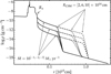 |
Fig. 1 Preshock breakout density profiles used as initial conditions for the radiation-hydrodynamics calculations. The model is for a progenitor star of 15 M⊙ initially and evolved at solar metallicity, which after explosion yielded an ejecta with a kinetic energy of 1.2 × 1051 erg. The CSM configurations are characterized by a different extent (RCSM values of 2, 6, and 10 × 1014 cm, indicated by solid, dotted, and dashed lines) and density (Ṁ values of 0.1, 0.01, and 0.001 M⊙yr−1). The same velocity law is used in all cases. For details, see Sect. 2. |
Summary of the CSM properties we adopted as initial conditions for our model grid.
3 Results from the radiation-hydrodynamics simulations with HERACLES
Figure 2 summarizes the results from the HERACLES simulations. It specifically shows the variations in peak bolometric luminosity relative to the rise time to peak, the time-integrated bolometric luminosity up to 15 d relative to the maximum ejecta velocity at 15 d, and the cold dense shell (CDS) velocity versus the CDS mass at 15 d (see also Table 2). Similar properties were shown in Dessart & Jacobson-Galán (2023) for a model set limited to just a few CSM (or associated mass-loss rate) configurations.
The wide range in ejecta kinetic energy of our model sample yields a broad range of outcomes (e.g., broader than in the simulations of Dessart & Jacobson-Galán 2023) because the ejecta kinetic energy is the energy source for the system (left panel of Fig. 2). The rise time to peak covers from a small fraction of a day (cases of small Ṁ, small RCSM, and high Ekin) to about 12 d, and reflects both the variation in shock-crossing time through the CSM and the diffusion time. The model ekin0p6_mdot0p1_rcsm1e15 has the longest rise time not only because the SN shock is slow to start with, but it is also strongly decelerated by a dense and extended CSM. The peak luminosity is typically about 1044 erg s−1. All else being kept the same, a greater RCSM or a greater M˙ have a qualitatively similar effect. The enhanced diffusion time tends to decrease Lpeak (the stored radiation energy is released over a longer duration), but the greater extraction of ejecta kinetic energy tends to increase Lpeak. The results in practice are case dependent, but in our simulations, all configurations with a CSM have a lower peak luminosity than in the No-CSM case (which is about 1045 erg s−1; the rise time in the No-CSM case is only about one hour and the peak is very narrow). For models mdot0p1 and rcsm1e15, the rise time is ∼10 d, and thus, the interaction is still ongoing at 15 d. These models belong to Type IIn SNe, in which interaction may continue for weeks and produce a superluminous transient.
Extraction of the ejecta kinetic energy implies a deceleration of the outer ejecta and a reduction of the maximum ejecta velocity (middle panel of Fig. 2). It covers from ~6300 to 3500 km s−1 in models with ekin0p6, from ∼9000 to 4800 km s−1 in models with ekin1p2, and from 11 500 to 5800 km s−1 in models with ekin1p8. All else being kept fixed, a greater CSM extent or higher mass causes a greater reduction in Vej,max,15d. Commensurate with this reduction of Vej,max,15d (or outer ejecta kinetic energy) is the time-integrated bolometric luminosity. In the ekin0p6 model set, the value relative to the No-CSM case (i.e., 4.39 × 1048 erg) spans from 4.75 × 1048 erg up to 3.19 × 1049 erg. In the ekin1p2 model set, the value relative to the No-CSM case (i.e., 7.67 × 1048 erg) spans from 8.35 × 1048 erg up to 6.42 × 1049 erg. In the ekin1p8 model set, the value relative to the No-CSM case (i.e., 1.08 × 1049 erg) spans from 1.22 × 1049 erg up to 1.28 × 1050 erg. In models mdot0p1 and rcsm1e15, the time-integrated bolometric luminosity still grows significantly at 15 d due to the persisting interaction (the value at 15 d may thus be close to or below that of the corresponding model with rcsm6e14).
The CDS mass at 15 d spans a wide range of values, from ∼0.01 M⊙ in the mdot0p001 cases (barely above the No-CSM case) to ∼1 M⊙ in the mdot0p1 cases, wherein the interaction is still ongoing at 15 d (right panel of Fig. 2). The greater the value of MCDS,15d, the lower the value of the CDS velocity at 15 d, which spans 6300 down to 3100 km s−1 in the model set ekin0p6, 8900 to 4300 km s−1 in the model set ekin1p2, and 11 300 to 5300 km s−1 in the model set ekin1p8.
Bolometric light curves for the full set of simulations with HERACLES are shown in Fig. 3. The morphology is similar in all cases, with a peak broadened over a diffusion time (i.e., broader for greater CSM mass or extent), and a luminosity that settles onto a ledge as the shock progresses through the outer regions of the dense CSM before marking an abrupt drop as the shock exits this dense CSM around RCSM. An interesting feature that is particularly visible in models mdot0p1 and rcsm1e15 is the break in light-curve slope that occurs after a few days, hence on the rise to peak, at a power of about 1042 erg s−1. This change in slope arises from the arrival (at the outer grid radius where the luminosity is recorded) of photons with a wavelength longer than the Balmer edge. It also coincides with the time when the CSM is ionized throughout. Thus, prior to this kink, the luminosity of the SN arises exclusively from low-energy (nonionizing) photons beyond 3670 Å, and the kink signals a sudden change not just in luminosity, but also in color (i.e., bluer) and ionization (i.e., ionized species start to appear). This transition may be at the origin of the similar light-curve kink and color change observed in SN 2024ggi (Shrestha et al. 2024a; Zhang et al. 2024; Jacobson-Galán et al. 2024a).
Although the dense CSM has been swept up in most simulations at 15 d (tag “Thin” in the column τCSM,15d), which corresponds to the end of the IIn phase (Dessart et al. 2017; Dessart & Jacobson-Galán 2023; Jacobson-Galán et al. 2024b), there remains some residual optically thick unshocked CSM in models mdot0p1 and rcsm1e15. In all other cases, the system is in the CDS phase, meaning that the photosphere (and the spectrum formation region) lies in the CDS (Dessart et al. 2016; Dessart 2026; Zheng et al. 2025). This is expected because even in RSG star explosions occurring in a vacuum, the photosphere lies no more than a few 0.01 M⊙ below the progenitor surface within the first 15 d after explosion (Bersten et al. 2011; Dessart & Hillier 2011).
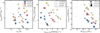 |
Fig. 2 Results from the radiation-hydrodynamics calculations for our sample of 27 ejecta and CSM configurations. Left: peak luminosity vs. rise time to peak. Middle: Time-integrated bolometric luminosity vs. maximum ejecta velocity, both evaluated at 15 d. Right: CDS velocity vs. CDS mass at 15 d. The colors signify different model kinetic energies, the symbols show the mass-loss rate, and the filling style shows the CSM extent. These indications, which apply to all panels, are given separately, one panel at a time for better visibility. For comparison, we also show the results for the three No-CSM cases (empty diamonds). The interaction phase is not concluded in models with a high CSM mass and extent, so the values are not yet converged at 15 d in these cases. |
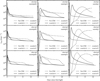 |
Fig. 3 Bolometric light curves calculated with the multigroup radiation-hydrodynamics code HERACLES and tiled according to the model ejecta kinetic energy (one value per row), CSM density (one value of M˙ per column), and CSM extent (three values per panel, with the No-CSM counterpart shown as a dotted line). The x-axis origin is chosen to be when each model first brightens to a luminosity of 1040 erg s−1, as recorded at the outer grid boundary. |
4 Multiband light curves computed with CMFGEN
In this section, we discuss the results from the radiative-transfer calculations performed with CMFGEN on selected snapshots of the 27 ejecta and CSM configurations modeled with HERACLES, with a focus on the photometric properties. As indicated in Sect. 2 and in Dessart et al. (2015, 2017), the Sobolev nonmonotonic-velocity solver in the NLTE code CMFGEN was used to postprocess the simulations from the radiation-hydrodynamics code HERACLES. Because the temperature structure is strongly affected by the dynamics (e.g., the location of the shock, its propagation, and the optical depth of the surrounding material), we imported this temperature in CMFGEN and held it fixed. Unlike HERACLES, however, which assumes LTE for the gas (e.g., its ionization level is fully known from the composition, the temperature, and the electron density), CMFGEN does not typically find that cooling and heating rates are equal with this adopted temperature. This inconsistency is the main reason for the systematic offset of up to about 80% of the luminosity obtained with CMFGEN compared to that of HERACLES for a given snapshot. Figure 4 illustrates this offset between the two codes for model ekin1p2_mdot0p01_rcsm6e14. Thus, the magnitudes obtained with CMFGEN are likely underestimated by 0.5–1.0 mag, and mostly in the UV range. We present a more quantitative discussion of this luminosity offset and its ramifications in Appendix C.
Figure 5 illustrates the UVW2-band light curves for the full model grid and using a similar tiling as for the bolometric light curves obtained with HERACLES and shown in Fig. 3. Compared to the No-CSM counterparts, models with interaction exhibit a significant boost to the UVW2 brightness and by extension to the UV luminosity, and the more so for denser and more extended CSM. Models with a modest CSM mass or extent peak at about −18.5 mag, whereas models with a high CSM mass or extent peak at about −20.5 mag. This boost persists for a few days in rcsm2e14 models but for one to two weeks in rcsm1e15 models. This overall pattern is mitigated by at least two factors, however. First, the diffusion of SN radiation through the optically thick CSM can delay the initial (i.e., the actual breakout) brightening by several days compared to the No-CSM counterpart, in which the breakout signal peaks within about an hour of shock emergence. The subsequent signal is then not just composed of the broadened diffuse breakout burst, but also augmented by the continuous supply of power from the interaction of the ejecta with this CSM, as well as the release of shock-deposited energy from the outermost ejecta layers. Second, the formation of the dense shell can lead to enhanced blanketing at later times that eventually causes a drop of the UVW2 brightness. This feature of the model is sensitive to the adopted CSM density profile; we imposed a strong and prompt reduction of the CSM density beyond RCSM. A more smoothly declining CSM density profile would produce a more smoothly declining UVW2-band brightness, as observed (Jacobson-Galán et al. 2024b).
Figure 5 indicates that the UVW2 brightness is a sensitive probe of ejecta interaction with the CSM, with a magnitude modulation that typically persists over the shock-crossing time through the dense CSM and scales by ≲1 mag, ~1.5 mag, and even ≳2 mag as the wind mass-loss rate is increased from 0.001 to 0.01 and 0.1 M⊙ yr−1. The results for the V-band light curves (shown in Fig. E.1) reveal a weaker effect of the CSM, likely because the optical range probes the Rayleigh–Jeans tail of the spectral energy distribution (i.e., the hot emitting plasma mostly radiates in the UV). Nonetheless, one important effect of the CSM is to shorten the rise time in the optical. The short V-band rise time of even standard Type II SNe suggests that some CSM, even if compact, is likely present in most or all exploding RSG stars (González-Gaitán et al. 2015; Morozova et al. 2017; Hinds et al. 2025).
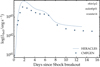 |
Fig. 4 Comparison between the HERACLES and CMFGEN bolometric light curves for model ekin1p2_mdot0p01_rcsm6e14. The HERACLES light curve has been shifted in time to correct for the light-travel time to the outer grid boundary. |
5 Results for the spectroscopic properties
In this section, we discuss the results from the radiative-transfer calculations performed with CMFGEN but with a focus on the spectral evolution for the full model grid. The main focus is on the IIn phase, which varies in duration depending on the ejecta kinetic energy, CSM mass, and extent of the configuration.
5.1 Hα as a diagnostic of the dynamics
In all the simulations we performed, the only line present and strong at all epochs (either in emission or absorption) was Hα (and to a lesser extent, Hβ). Compared to other species, there is only one higher-ionization state (the same applies to He II), and consequently, H I lines are present regardless of the ionization level or temperature of the gas. This property also implies that H I lines might form over a wide range of depths even in the presence of an ionization stratification. These properties thus make Hα an ideal diagnostic of the dynamics of the interaction of SN ejecta with the CSM. We primarily focus the discussion on the broad component of Hα, as would be observed in low-resolution spectra. The narrow component (observable in high-resolution spectra) is discussed in Dessart (2025).
Figure 6 illustrates in the left column the Hα evolution in model ekin1p2_mdot0p01_rcsm6e14 over the first week as the SN evolves through the IIn phase (first two epochs) into the CDS phase (last two epochs), together with the corresponding ejecta and CSM structure (velocity, density, and temperature) from the HERACLES simulation at the corresponding epoch in the right column. Using a colored shading, we indicate the spatial regions (right) at the origin of the emission or absorption regions in Hα (left). For the first epoch, Hα exhibits a symmetric electron-scattering broadened emission profile with a narrow core. The flux in the extended line wings arises from slow-moving (<50 km s−1) relatively cool (~10 000 K) unshocked CSM wherein the radiation from the shock is absorbed and reemitted, as well as scattered by free electrons. The narrow-line core arises from an external region at a low electron-scattering optical depth where photons are essentially not redistributed in frequency by free electrons. Thus, at this first epoch, the entire line emission arises from unshocked CSM. Radiative acceleration of the unshocked CSM also leads to the disappearance of the SN shock at this early time.
At the second epoch of 2.5 d shown in the second row of Fig. 6, the configuration is essentially unchanged, except for a clear radiative acceleration of the unshocked CSM, with velocities as high as ∼2000 km s−1 at τ ∼ 10 (just exterior to the SN shock, which is now visible), 220 km s−1 at τ ~ 0.1, and 170 km s−1 at τ ∼ 0.01, where the narrow-line core (though now broadened) forms (see discussion in Dessart 2025).
At the third epoch of 5.0 d shown in the third row of Fig. 6, the configuration is now qualitatively changed because the profile combines emission from unshocked CSM (whose volume decreased due to the shock expansion) and absorption from the fast-moving dense shell located at an optical depth of a few (red shading). This well-formed dense shell is easily identifiable as the density bump with a representative velocity of 6000 km s−1 (right column of Fig. 6).
At the last epoch of 6.67 d shown in the bottom row of Fig. 6, the unshocked CSM is now entirely optically thin (in electron scattering) and only contributes narrow emission at the line center. The SN radiation, however, has accelerated this material around τ = 0.01 up to 500 km s−1, so that this narrow-line core is much broader than in the first epoch (top row). The bulk of the spectrum (around the photosphere) now forms in the dense shell (red shading), causing an extended absorption out to −6000 km s−1 on the blue side of the Hα profile.
Our set of 27 models exhibits evolving dynamical configurations and thus evolving Hα profile morphologies, but the basic features discussed above apply in all cases. In the appendix, we show in Fig. E.2 the corresponding results for model ekin1p2_mdot0p1_rcsm2e14, in which the high CSM density but smaller CSM extent lead to a much stronger radiative acceleration of the unshocked material (see discussion in Dessart 2025). This acceleration is so strong that the SN shock essentially disappears during the first few days after the shock crosses the progenitor R∗. It leads to Hα emission out to about 4000 km s−1, essentially all blueshifted relative to the line center because of optical depth effects.
The Hα evolution observed in SN 1998S (Leonard et al. 2000; Fassia et al. 2001) shows a qualitatively similar behavior to that shown above for model ekin1p2_mdot0p01_rcsm6e14, with a somewhat longer IIn phase of about a week and a prolonged CDS phase lasting until about three weeks. The high CDS mass in SN 1998S facilitates the identification of the blueshifted absorption from the CDS, which is observed simultaneously at day 25 (see Fig. 5 of Leonard et al. 2000) with the narrow emission and absorption from distant unshocked CSM. More frequently, this hybrid profile morphology is less obvious (see, e.g., for SNe 2023ixf and 2024ggi; Bostroem et al. 2023; Jacobson-Galán et al. 2023; Singh et al. 2024; Jacobson-Galán et al. 2024a; Zhang et al. 2024; Zheng et al. 2025), which may arise from a combination of a lower CDS mass and departures from spherical symmetry, as well as insufficient data quality (i.e., signal-to-noise ratio and spectral resolution).
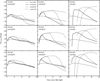 |
Fig. 5 Same as Fig. 3, but now showing the UVW2-band light curves computed with CMFGEN for our model set. |
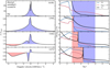 |
Fig. 6 Correspondence between the Hα evolution (left column; only H I lines are included in the displayed range) and the dynamical properties in the spectrum formation region (right column) for model ekin1p2_mdot0p01_rcsm6e14. The shading differentiates emission from the unshocked CSM (blue) and the shocked material (red), which corresponds here to the dense shell. The spectrum forms preferentially over regions in which log τ is between −1 and 1, except for the narrow-line core arising from regions at log τ of about −2. Here, V8 refers to the velocity in units of 108 cm s−1 and T4 is the gas (or electron) temperature in units of 104 K (log ρ is the base-10 logarithm of the density, shown with an additive constant for better visibility). |
5.2 Lines of He, C, N, and O as diagnostics of the ionization evolution
Shock breakout from a RSG star is an extreme phenomenon that causes a change in the surface temperature of the exploded star from a few 103 to about 105 K, although this jump is reduced for a higher CSM mass or extent (Moriya et al. 2011; Dessart et al. 2017); this breakout phase also comes with a change in luminosity by a factor of ∼105, leading to a sudden and extended migration of the exploded star in the Hertzsprung–Russell diagram. With our set of 27 different ejecta and CSM configurations, we obtained a high diversity, as evidenced by the range in peak luminosities, rise times, or time-integrated bolometric luminosity (see Table 2 and Fig. 2). In this section, we turn to the corresponding spectral changes, in particular, we study the variation in the emission lines during the IIn phase in nature and strength. The IIn phase corresponds to all times when some optically thick unshocked although potentially radiatively accelerated CSM remained.
To conduct this analysis, we produced rectified spectra for all configurations and epochs (corresponding to a total of about 500 individual spectra). For each model set, we noted the epochs over which we were able to identify the presence of He I 5875.66 Å, He II 4685.70 Å, C III 5695.92 Å, C IV 5804.86 Å, “N III–C III” (this term corresponds here to the blend of multiplets due to both N III and C III, and in particular, N III 4640.64 Å and C III 4647.42 Å), N IV 7109.35 Å, N V 4612.72 Å, O V 5597 Å, and O VI 3820 Å. The results from this analysis are stored in Table A.1. These results have obvious limitations because the spectral sequences only inform us on the actual times of the computed spectra. In particular, computations at the earliest times when the CSM is still cold are challenging, so we make no claim on the presence or absence of any lines prior to the first spectrum of each sequence. Finally, we tried to use a high enough cadence to properly sample the spectral evolution. A higher cadence (meaning computing many more models and their spectra; doubling the cadence would mean computing 1000 models rather than 500) might reveal more subtle variations in some cases.
The first fundamental property of all simulations is the systematic rise and decline in ionization through the shock-breakout phase and beyond. This is easily explained from the preSN conditions characterized by a cool RSG atmosphere and CSM, the progressive heating and photoionization of this environment during breakout and shock propagation, and eventually, the cooling and recombination of this material (CSM or shocked ejecta and CSM) through expansion and radiative losses. As long at the SN shock is deeply embedded in the optically thick unshocked CSM, the optical depth in the Lyman continuum and X-ray range is gigantic (i.e., the associated opacities are many orders of magnitude greater than that of electron scattering). Hence, photoionization during the IIn phase is entirely controlled by secondary photons, that is, by photons emitted within the CSM. All primary photons from the SN shock are essentially absorbed on the spot. This photoionization is then caused by (quasi) black-body radiation at an equilibrium temperature of a few 104 K, and this gas or radiation temperature in the optically thick CSM arises from the absorption of radiation and particles emitted by the shock (gas properties from HERACLES simulations of similar configurations are shown in Dessart et al. 2015, 2017; Dessart & Jacobson-Galán 2023).
Because of this rise and decline in ionization, the He lines of the model spectra evolve with He I → He II He I (and eventually, no He I lines at all), C lines with C III → C IV C → III (and eventually, no C lines, at least in the optical), N lines with N III → N IV → NV → N IV → N III (and eventually, no N lines at all). For O, the situation is more complicated since the models tend to only predict lines of OV and OVI (i.e., O V 5597 Å and O VI 3820 Å), so they are only present when the ionization (or temperature) is high. To observe this sequence in ionization (i.e., rise and decline) rather than a continuous decline requires an early discovery and prompt spectroscopic follow-up, and this was successfully achieved for SN 2024ggi (see, e.g., Zhang et al. 2024) and was obtained here in models rcsm6e14 and mdot0p01/mdot0p1. In some events characterized by a confined CSM, the surge in ionization is so short that only a decline can be observed (see, e.g., SN 2013fs; Yaron et al. 2017), as in models rcsm2e14 or mdot0p001 (i.e., computing models prior to this phase of high ionization is numerically challenging). At the opposite end (i.e., dense and very extended CSM), the ionization change through the shock-breakout phase is much more moderate, with species remaining once or twice ionized at most (in the optical range). Finally, our simulations do not typically predict the simultaneous presence of lines (of a given element) from two consecutive ionization levels, such as N III and N IV lines or OV and OVI lines (there are some exceptions; e.g., model ekin1p2_mdot0p01_rcsm2e14 at 1 d and shown in Fig. 7). This mostly arises from the fact that although the unshocked CSM might have an ionization stratification, the bulk of the emission arises from a region of essentially uniform ionization. A natural way to break this property is asymmetry, as might result from an asymmetric shock breakout or an asymmetric stellar environment (see, e.g., Gabler et al. 2021; Goldberg et al. 2022b; Vartanyan et al. 2025).
A related feature is that lines arising from ions that have a similar ionization potentials tend to be present at the same epochs. Again, this does not apply to H I lines, which are present regardless of the ionization level, and thus, in all model configurations and epochs. He I lines tend to be present along with N III lines, however. He II lines (just like H I lines) are present over a wide range, although of relatively high ionization (e.g., present together with N III, N IV, or NV lines). N IV lines tend to be present along with C IV lines, and for the same reason, NV lines tend to be present along with OV lines (there are no CV lines because of the huge associated ionization potential). Throughout our full set, the ion that is only present for the highest ionizations is OVI. In models with a CSM, we find that the temperature/ionization of the unshocked CSM is never high enough to produce complete ionization, so the optical spectra are never featureless (this occurs at the earliest post-breakout times in the No-CSM models).
Following Table A.1, we can discuss the spectral properties during the IIn phase in terms of explosion or CSM properties more specifically. The presence of He I lines such as He I 5875.66 Å is favored in models with a dense and extended CSM (model mdot0p1 and rcsm1e15), or a low explosion energy; He I lines are present at later times when He II disappears, but this tends to occur in these cases during the CDS phase or after. He II lines are present in all models at some stage, but its subsistence requires high ionization, so it vanishes more quickly in models with a lower explosion energy. In models with a compact CSM (i.e., rcsm2e14), the ionization is high throughout the IIn phase in essentially all cases, and thus, electron-scattering broadened He II 4685.70 Å is present (the weaker line He II 5411.52 Å is also a useful diagnostic because it is isolated). C III 5695.92 Å is typically rarely seen and quite weak, and instead, all models predict strong C IV 5804.86 Å at some stage in the IIn phase, essentially for a subset of the epochs at which He II 4685.70 Å is also predicted. N III lines are mostly present in models with massive extended CSM (rcsm6e14 and rcsm1e15 or mdot0p1), and it tends to be present early on and later on following the rise and fall of the ionization. The strongest N III line in the optical (i.e., N III 4640.64 Å) produces an emission bump on the blue side of He II 4685.70 Å, but our models predict even more flux from the overlapping contribution due to C III 4647.42 Å (this finding is not surprising given the presence of both N IV 7109.35 Å and C IV 5804.86 Å at some epochs and despite the overabundance of N relative to C). The models predict N IV lines unless the ionization remains too low (i.e., cases of dense or extended CSM). NV and OV lines require high gas ionization, and thus, they shy away from the cases of dense and extended CSM. A higher kinetic energy boosts the CSM ionization and favors their presence. The most extreme of all is O VI 3820 Å, which is the most short-lived of all lines and requires the highest ionization. This situation is only met for a compact and tenuous CSM. Such a CSM tends to be optically thin sooner or strongly radiatively accelerated, so seeing an electron-scattering broadened O VI 3820 Å is challenging.
To summarize some of these properties, Fig. 7 presents a selection of spectra from different ejecta and CSM configurations and post-breakout epochs and stacked in order of increasing ionization from top to bottom. At the top, a cool model spectrum shows the simultaneous presence of He I, C III, and N III lines (model ekin0p6_mdot0p1_rcsm1e15 at 10 d), followed by a warm model spectrum having He II, C IV and N IV lines (model ekin1p2_mdot0p01_rcsm6e14 at 2.5 d), then a warm/hot model spectrum with He II, NV and OV lines (model ekin1p8_mdot0p001_rcsm6e14 at 12 hr), and then two hot model spectra with simultaneously NV, OV, and OVI (model ekin1p2_mdot0p01_rcsm2e14 at 1 d) or just OVI (model ekin1p8_mdot0p001_rcsm2e14 at 8 hr). As described above, H I lines (and He II lines to a smaller extent) tend to be present over a wide range of ionization and temperature.
Light-curve and ejecta properties from the HERACLES simulations for our model grid.
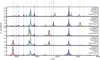 |
Fig. 7 Spectral morphology during the IIn phase that results from a range of ionization of the unshocked CSM, from cool weakly ionized conditions at the top to hot and highly ionized conditions at the bottom. The models shown here differ in ejecta and CSM configuration and in post-breakout time. In all cases, He II 6560.1 Å is a contaminant to the Hα emission. |
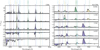 |
Fig. 8 Comparison of the spectral evolution of model ekin1p2 with a CSM (left; case mdot0p01 and rcsm6e14) and without CSM (right). The rest wavelength of the main lines is indicated and is also color-coded to differentiate different species. The lines that are affected by Doppler broadening exhibit a strong blueshift and can primarily appear in absorption (later epochs in the CSM case during the CDS phase) or primarily in emission (No-CSM case). See Sect. 5.3 for a discussion. |
5.3 Comparison of results for configurations with and without CSM
In the preceding sections, we have discussed the effect of the CSM on the dynamical and radiative properties of our Type II SN models. Corresponding results were compared to the No-CSM case in Fig. 2 (empty diamond symbols), as well as Figs. 3–5 (dotted lines) and are stored in Table 2. We discuss the contrast in the associated spectroscopic properties in detail below.
Figure 8 illustrates the fundamental change in spectral evolution, and in particular, in the level of ionization and line profile morphology when a CSM is present and instead when the RSG star explodes in a vacuum (the CSM model used here is ekin1p2_mdot0p01_rcsm6e14, and the No-CSM counterpart just adopts a uniform wind mass-loss rate of 10−6 M⊙ yr−1). These results were already shown and discussed in Dessart et al. (2017) with models r1w1 (wind mass-loss rate of 10−6 M⊙ yr−1) and, for example, r1w6 (high-mass CSM density corresponding to a wind mass-loss rate of 10−2 M⊙ yr−1), but are repeated here and reinforced with a more direct comparison. Our results are still the same in nature as those from 10 years ago.
The first important prediction is the presence of lines from ionized species in both cases. In contrast to common belief, the highest ionization is reached in the model without CSM, but it is short-lived. For example, at 16 hr, the No-CSM model exhibits lines of C IV and N IV, at a time when the model with a CSM is cool and mostly shows lines of He I. The No-CSM model eventually cools and exhibits lines of C III and N III, followed after a few days by lines mostly of H I and He I. In contrast, the model with a CSM heats up during the first 1–2 days, switching from He I to He II lines and so on, followed at later times after some cooling and recombination to a spectrum with He I lines and H I lines only, as in the No-CSM case. The different evolution followed by each model reflects the complex interplay between expansion and radiative cooling, on the one hand, and photo-ionization heating, on the other hand (for the CSM case). Clearly, however, the presence of He II 4685.70 Å is common to both CSM and No-CSM cases. This line has been observed for decades, and models without CSM could explain its presence at early times in SN 2006bp or SN 1999gi (Dessart et al. 2008). Today, it is often referred to as a ledge feature (see, e.g., Hosseinzadeh et al. 2022, Pearson et al. 2023, Shrestha et al. 2024b).
The other difference, which is more striking, concerns the line profile morphology. With a CSM, the model exhibits IIn signatures as long as there is an optically thick unshocked CSM, followed by a phase during which the spectrum is quasi-featureless (i.e., when the photosphere is in the CDS). Over the 15 d period shown, all lines evolve from having a narrow core with symmetric extended wings that are electron-scattering broadened to being Doppler broadened with mostly blueshifted absorption. In contrast, without a CSM, the lines are broad, Doppler broadened, and strongly blueshifted immediately at shock breakout as the progenitor surface is promptly accelerated after shock passage (the No-CSM model is in the ejecta phase at all epochs). This blueshift of all lines is an optical depth effect and persists until the end of the photospheric phase, hence for several months in a typical Type II plateau SN (Dessart & Hillier 2005; Anderson et al. 2014).
The differences in profile morphology between the CSM and No-CSM cases are not limited to the initial 15 d covered by Fig. 8. Models predict that differences persist at later times (Hillier & Dessart 2019), with a bluer optical color and an excess Hα emission with reduced absorption (see also, e.g., Gutiérrez et al. 2014, 2017b,a). Additional signatures such as a UV excess might arise when weak power is injected in the outer ejecta by persisting interaction with the progenitor wind (Dessart & Hillier 2022; Dessart et al. 2023; Jacobson-Galán et al. 2024b), as observed in SN 2023ixf (Bostroem et al. 2024, 2025; Jacobson-Galán et al. 2025). When the (outer) ejecta structure has been modified by interaction with the CSM, it indeed carries the imprint of this interaction for weeks, months, and years, and this is typically only modified by further interaction with additional CSM at greater distances.
6 Conclusions
We have presented radiation-hydrodynamics and radiative-transfer calculations of Type II SNe interacting with the CSM with a focus on the first 15 d after the SN shock crosses R∗. Compared to our previous work, we covered a broader range of explosion and CSM properties in a systematic way, specifically, by modeling the explosion of a 15 M⊙ star characterized by an ejecta kinetic energy of 0.6, 1.2, and 1.8 × 1051 erg, a CSM corresponding to a wind mass-loss rate of 0.001, 0.01, and 0.1 M⊙ yr−1, and a CSM extent of 2, 6, and 10 1014 cm. The results of this work agree with Dessart et al. (2017) and Dessart & Jacobson-Galán (2023), but this new extended regular grid of models offers an unprecedented treasury for the analysis of future observations. A brief comparison of these simulations to observations is presented in Appendix B. Additional information on the numerical setup, approximations, and limitations is provided in Appendices C and D.
Compared to explosions in a vacuum (i.e., the No-CSM counterpart), the presence of the CSM alters the dynamics and the escaping radiation from the SN by reducing the peak luminosity, broadening the light curve, and potentially extending the initial high-brightness phase through the extraction of ejecta kinetic energy. Consequently, decelerated ejecta material and swept-up CSM pile up into a dense shell, whose velocity is slightly lower than the maximum ejecta velocity. We discussed the relation of these various quantities to each other. A wide range of radiative acceleration of the unshocked CSM was also obtained.
We illustrated the importance of Hα for inferring the dynamical evolution of the interaction, in part because H I lines are present regardless of the ionization. High-cadence monitoring, preferentially at high or moderate spectral resolution, can provide information on the size and density of the optically thick CSM during the IIn phase, the velocity and mass of the dense shell in the CDS phase, or the acceleration of the unshocked CSM located at and beyond the photosphere.
We also described the potential range in spectral diversity during the IIn phase, which is primarily driven by the variation in ionization of the unshocked CSM. These modulations in ionization are a function of the post-breakout time, the CSM density and extent, and of the explosion energy, such that much degeneracy prevails. With our model grid, we identified spectral properties reflecting a low ionization (He I and N III lines), a moderate ionization (He II, C IV, and N IV lines), a high ionization (He II, CV, and NV), and a very high ionization (He II and OVI lines). We found that lines of C, N, and O are systematically present at the same time (e.g., C IV 5804.86 Å and N IV 7109.35 Å) because of the similarity in the corresponding ionization potential and despite the differences in abundances. We also found that N III 4640.64 Å and C III 4647.42 Å are both contributors to the narrow emission on the blue side of He II 4685.70 Å.
Finally, we commented on the critical differences brought in with the presence of the CSM. With the CSM, the rise in ionization is delayed and the evolution of the profile morphology exhibits at least three phases (IIn phase, CDS phase, and ejecta phase; see also Dessart 2026); our simulations were mostly limited to the first two phases. During the IIn phase, the line profiles all exhibit symmetric emission with a narrow core and extended electron-scattering broadened wings. During the CDS phase, the profiles are hybrid, with a narrow P-cygni profile near the line center from the distant unshocked CSM and a blueshifted absorption arising from the CDS. In contrast, without the CSM, the rise in ionization is prompt and the profile morphology is immediately dominated by Doppler-broadened lines with a strong blueshift caused by optical depth effects. In particular, He II 4685.70 Å is present in both the CSM and No-CSM cases, but it is systematically broad and blueshifted in the No-CSM case.
Our work has a number of limitations. The radiative transfer technique uses the Sobolev approximation. We also adopted the temperature structure from HERACLES in order to capture the temperature structure, controlled by the dynamics and the presence of the shock, but this temperature is compromised by the assumption of LTE for the gas (e.g., Saha ionization equilibrium) in HERACLES. We also adopted a parametrized approach in which the ejecta kinetic energy, the CSM mass, and the CSM extent were set without any global physical consistency. For example, the wind mass loss might be higher in higher-mass progenitors, whereas we used a fixed progenitor mass of 15 M⊙ for all simulations. The wind mass loss might also correlate with the preSN mass, for example, enhanced mass loss producing partially stripped progenitors. The underlying assumption here was that regardless of the adopted mass loss, only negligible stripping results. Resolving these limitations will require code developments, but also a much better understanding of mass loss in massive stars. Until then, a parameterized approach is the only practical way to proceed.
Data availability
These simulations will be compared to the current sample of SNe II exploding in CSM in Jacobson-Galán et al. (in prep.) and subsequently uploaded at https://zenodo.org/communities/snrt as tar-zipped multicolumn ascii files. This includes the results from the radiation-hydrodynamics calculations (light curves and dynamical properties) and the results from the NLTE radiative transfer (light curves and multi-epoch spectra) for the whole model set with and without a CSM (i.e., 30 configurations).
Acknowledgements
LD acknowledges support from the ESO Scientific Visitor Program for a visit to ESO-Garching during the summer 2025. This work was granted access to the HPC resources of TGCC under the allocation 2024 – A0170410554 on Irene-Rome made by GENCI, France. This research has made use of NASA’s Astrophysics Data System Bibliographic Services.
References
- Anderson, J. P., Dessart, L., Gutierrez, C. P., et al. 2014, MNRAS, 441, 671 [NASA ADS] [CrossRef] [Google Scholar]
- Bersten, M. C., Benvenuto, O., & Hamuy, M. 2011, ApJ, 729, 61 [NASA ADS] [CrossRef] [Google Scholar]
- Blondin, S., Blinnikov, S., Callan, F. P., et al. 2022, A&A, 668, A163 [NASA ADS] [CrossRef] [EDP Sciences] [Google Scholar]
- Boian, I., & Groh, J. H. 2020, MNRAS, 496, 1325 [CrossRef] [Google Scholar]
- Bostroem, K. A., Pearson, J., Shrestha, M., et al. 2023, ApJ, 956, L5 [NASA ADS] [CrossRef] [Google Scholar]
- Bostroem, K. A., Sand, D. J., Dessart, L., et al. 2024, ApJ, 973, L47 [NASA ADS] [CrossRef] [Google Scholar]
- Bostroem, K. A., Valenti, S., Sand, D. J., et al. 2025, ApJ, submitted [arXiv:2508.11756] [Google Scholar]
- Bronner, V. A., Laplace, E., Schneider, F. R. N., & Podsiadlowski, P. 2025, A&A, 703, A61 [NASA ADS] [CrossRef] [EDP Sciences] [Google Scholar]
- Bruch, R. J., Gal-Yam, A., Schulze, S., et al. 2021, ApJ, 912, 46 [NASA ADS] [CrossRef] [Google Scholar]
- Bruch, R. J., Gal-Yam, A., Yaron, O., et al. 2023, ApJ, 952, 119 [NASA ADS] [CrossRef] [Google Scholar]
- Chugai, N. N. 2001, MNRAS, 326, 1448 [NASA ADS] [CrossRef] [Google Scholar]
- Davies, B., & Dessart, L. 2019, MNRAS, 483, 887 [NASA ADS] [CrossRef] [Google Scholar]
- Dessart, L. 2025, A&A, 694, A132 [NASA ADS] [CrossRef] [EDP Sciences] [Google Scholar]
- Dessart, L. 2026, Encyclopedia of Astrophysics, 2, 706 [Google Scholar]
- Dessart, L., & Hillier, D. J. 2005, A&A, 437, 667 [NASA ADS] [CrossRef] [EDP Sciences] [Google Scholar]
- Dessart, L., & Hillier, D. J. 2011, MNRAS, 410, 1739 [NASA ADS] [Google Scholar]
- Dessart, L., & Hillier, D. J. 2022, A&A, 660, L9 [NASA ADS] [CrossRef] [EDP Sciences] [Google Scholar]
- Dessart, L., & Jacobson-Galán, W. V. 2023, A&A, 677, A105 [NASA ADS] [CrossRef] [EDP Sciences] [Google Scholar]
- Dessart, L., Blondin, S., Brown, P. J., et al. 2008, ApJ, 675, 644 [NASA ADS] [CrossRef] [Google Scholar]
- Dessart, L., Hillier, D. J., Gezari, S., Basa, S., & Matheson, T. 2009, MNRAS, 394, 21 [NASA ADS] [CrossRef] [Google Scholar]
- Dessart, L., Livne, E., & Waldman, R. 2010, MNRAS, 405, 2113 [NASA ADS] [Google Scholar]
- Dessart, L., Audit, E., & Hillier, D. J. 2015, MNRAS, 449, 4304 [Google Scholar]
- Dessart, L., Hillier, D. J., Audit, E., Livne, E., & Waldman, R. 2016, MNRAS, 458, 2094 [Google Scholar]
- Dessart, L., Hillier, D. J., & Audit, E. 2017, A&A, 605, A83 [NASA ADS] [CrossRef] [EDP Sciences] [Google Scholar]
- Dessart, L., John Hillier, D., & Kuncarayakti, H. 2022, A&A, 658, A 130 [Google Scholar]
- Dessart, L., Gutiérrez, C. P., Kuncarayakti, H., Fox, O. D., & Filippenko, A. V. 2023, A&A, 675, A33 [NASA ADS] [CrossRef] [EDP Sciences] [Google Scholar]
- Dessart, L., Leonard, D. C., Vasylyev, S. S., & Hillier, D. J. 2025, A&A, 696, L12 [NASA ADS] [CrossRef] [EDP Sciences] [Google Scholar]
- Ercolino, A., Jin, H., Langer, N., & Dessart, L. 2024, A&A, 685, A58 [NASA ADS] [CrossRef] [EDP Sciences] [Google Scholar]
- Fassia, A., Meikle, W. P. S., Vacca, W. D., et al. 2000, MNRAS, 318, 1093 [Google Scholar]
- Fassia, A., Meikle, W. P. S., Chugai, N., et al. 2001, MNRAS, 325, 907 [NASA ADS] [CrossRef] [Google Scholar]
- Fuller, J. 2017, MNRAS, 470, 1642 [NASA ADS] [CrossRef] [Google Scholar]
- Fuller, J., & Tsuna, D. 2024, Open J. Astrophys., 7, 47 [CrossRef] [Google Scholar]
- Gabler, M., Wongwathanarat, A., & Janka, H.-T. 2021, MNRAS, 502, 3264 [CrossRef] [Google Scholar]
- Gal-Yam, A., Kasliwal, M. M., Arcavi, I., et al. 2011, ApJ, 736, 159 [NASA ADS] [CrossRef] [Google Scholar]
- Goldberg, J. A., Jiang, Y.-F., & Bildsten, L. 2022a, ApJ, 929, 156 [NASA ADS] [CrossRef] [Google Scholar]
- Goldberg, J. A., Jiang, Y.-F., & Bildsten, L. 2022b, ApJ, 933, 164 [NASA ADS] [CrossRef] [Google Scholar]
- González, M., Audit, E., & Huynh, P. 2007, A&A, 464, 429 [Google Scholar]
- González-Gaitán, S., Tominaga, N., Molina, J., et al. 2015, MNRAS, 451, 2212 [CrossRef] [Google Scholar]
- Groh, J. H. 2014, A&A, 572, L11 [NASA ADS] [CrossRef] [EDP Sciences] [Google Scholar]
- Gutiérrez, C. P., Anderson, J. P., Hamuy, M., et al. 2014, ApJ, 786, L15 [CrossRef] [Google Scholar]
- Gutiérrez, C. P., Anderson, J. P., Hamuy, M., et al. 2017a, ApJ, 850, 90 [CrossRef] [Google Scholar]
- Gutiérrez, C. P., Anderson, J. P., Hamuy, M., et al. 2017b, ApJ, 850, 89 [CrossRef] [Google Scholar]
- Hillier, D. J., & Miller, D. L. 1998, ApJ, 496, 407 [NASA ADS] [CrossRef] [Google Scholar]
- Hillier, D. J., & Dessart, L. 2012, MNRAS, 424, 252 [CrossRef] [Google Scholar]
- Hillier, D. J., & Dessart, L. 2019, A&A, 631, A8 [NASA ADS] [CrossRef] [EDP Sciences] [Google Scholar]
- Hosseinzadeh, G., Kilpatrick, C. D., Dong, Y., et al. 2022, ApJ, 935, 31 [NASA ADS] [CrossRef] [Google Scholar]
- Irani, I., Morag, J., Gal-Yam, A., et al. 2024, ApJ, 970, 96 [Google Scholar]
- Jacobson-Galán, W. V., Dessart, L., Jones, D. O., et al. 2022, ApJ, 924, 15 [CrossRef] [Google Scholar]
- Jacobson-Galán, W. V., Dessart, L., Margutti, R., et al. 2023, ApJ, 954, L42 [CrossRef] [Google Scholar]
- Jacobson-Galán, W. V., Davis, K. W., Kilpatrick, C. D., et al. 2024a, ApJ, 972, 177 [CrossRef] [Google Scholar]
- Jacobson-Galán, W. V., Dessart, L., Davis, K. W., et al. 2024b, ApJ, 970, 189 [CrossRef] [Google Scholar]
- Jacobson-Galán, W. V., Dessart, L., Kilpatrick, C. D., et al. 2025, ApJ, 994, L14 [Google Scholar]
- Kasliwal, M. M., Bellm, E., & Graham, M. 2025, Trans. Name Server AstroNote, 238, 1 [Google Scholar]
- Kulkarni, S. R., Harrison, F. A., Grefenstette, B. W., et al. 2021, arXiv e-prints [arXiv:2111.15608] [Google Scholar]
- Kumar, A., Dastidar, R., Maund, J. R., Singleton, A. J., & Sun, N.-C. 2025, MNRAS, 538, 659 [Google Scholar]
- Leonard, D. C., Filippenko, A. V., Barth, A. J., & Matheson, T. 2000, ApJ, 536, 239 [Google Scholar]
- Livne, E. 1993, ApJ, 412, 634 [Google Scholar]
- Ma, J.-Z., Chiavassa, A., de Mink, S. E., et al. 2024, ApJ, 962, L36 [NASA ADS] [CrossRef] [Google Scholar]
- Ma, J.-Z., Justham, S., Pakmor, R., et al. 2025, ApJ, submitted [arXiv:2510.14875] [Google Scholar]
- Moriya, T., Tominaga, N., Blinnikov, S. I., Baklanov, P. V., & Sorokina, E. I. 2011, MNRAS, 415, 199 [NASA ADS] [CrossRef] [Google Scholar]
- Morozova, V., Piro, A. L., & Valenti, S. 2017, ApJ, 838, 28 [NASA ADS] [CrossRef] [Google Scholar]
- Niemela, V. S., Ruiz, M. T., & Phillips, M. M. 1985, ApJ, 289, 52 [NASA ADS] [CrossRef] [Google Scholar]
- Paxton, B., Bildsten, L., Dotter, A., et al. 2011, ApJS, 192, 3 [Google Scholar]
- Paxton, B., Cantiello, M., Arras, P., et al. 2013, ApJS, 208, 4 [Google Scholar]
- Paxton, B., Marchant, P., Schwab, J., et al. 2015, ApJS, 220, 15 [Google Scholar]
- Pearson, J., Hosseinzadeh, G., Sand, D. J., et al. 2023, ApJ, 945, 107 [NASA ADS] [CrossRef] [Google Scholar]
- Roussel-Hard, L., Audit, E., Dessart, L., Padioleau, T., & Wang, Y. 2025, A&A, 696, A201 [NASA ADS] [CrossRef] [EDP Sciences] [Google Scholar]
- Schlegel, E. M. 1990, MNRAS, 244, 269 [NASA ADS] [Google Scholar]
- Shiode, J. H., & Quataert, E. 2014, ApJ, 780, 96 [Google Scholar]
- Shivvers, I., Groh, J. H., Mauerhan, J. C., et al. 2015, ApJ, 806, 213 [NASA ADS] [CrossRef] [Google Scholar]
- Shrestha, M., Bostroem, K. A., Sand, D. J., et al. 2024a, ApJ, 972, L15 [Google Scholar]
- Shrestha, M., Pearson, J., Wyatt, S., et al. 2024b, ApJ, 961, 247 [Google Scholar]
- Shvartzvald, Y., Waxman, E., Gal-Yam, A., et al. 2024, ApJ, 964, 74 [NASA ADS] [CrossRef] [Google Scholar]
- Singh, A., Teja, R. S., Moriya, T. J., et al. 2024, ApJ, 975, 132 [CrossRef] [Google Scholar]
- Soker, N. 2021, ApJ, 906, 1 [Google Scholar]
- Terreran, G., Jacobson-Galán, W. V., Groh, J. H., et al. 2022, ApJ, 926, 20 [NASA ADS] [CrossRef] [Google Scholar]
- Vartanyan, D., Tsang, B. T. H., Kasen, D., et al. 2025, ApJ, 982, 9 [Google Scholar]
- Vaytet, N. M. H., Audit, E., Dubroca, B., & Delahaye, F. 2011, J. Quant. Spec. Radiat. Transf., 112, 1323 [NASA ADS] [CrossRef] [Google Scholar]
- Yaron, O., Perley, D. A., Gal-Yam, A., et al. 2017, Nat. Phys., 13, 510 [NASA ADS] [CrossRef] [Google Scholar]
- Yoon, S.-C., & Cantiello, M. 2010, ApJ, 717, L62 [NASA ADS] [CrossRef] [Google Scholar]
- Zhang, J., Wang, X., József, V., et al. 2020, MNRAS, 498, 84 [NASA ADS] [CrossRef] [Google Scholar]
- Zhang, J., Dessart, L., Wang, X., et al. 2024, ApJ, 970, L18 [NASA ADS] [CrossRef] [Google Scholar]
- Zheng, W., Dessart, L., Filippenko, A. V., et al. 2025, ApJ, 988, 61 [Google Scholar]
Other values of v∞ and different acceleration length scales were studied in Dessart (2025), but have little importance for the present work, in which we focus on the information encoded in moderate- to low-resolution spectra. Furthermore, configurations with the same  yield the same light curve and spectral evolution because primarily, the CSM density matters.
Appendix A Summary table of spectral-line diagnostics
Table A.1 presents a summary of spectral-line diagnostics for our 27 ejecta and CSM configurations. For each model set, we noted the epochs over which we were able to identify the presence of He I 5875.66 Å, He II 4685.70 Å, C III 5695.92 Å, C IV 5804.86 Å, “N III–C III” (this term corresponds here to the blend of multiplets due to both N III and C III, and in particular, N III 4640.64 Å and C III 4647.42 Å), N IV 7109.35 Å, N V 4612.72 Å, O V 5597 Å, and O VI 3820 Å.
Appendix B Comparison to observations
While the detailed comparison of these simulations to observations is deferred to Jacobson-Galán et al. (in prep), we show in Fig. B.1 the broad compatibility with the distribution of SNe II that exhibit signatures of interaction in their multiband light curves and spectra. This is not surprising given that the current set of simulations is merely an extension of previous similar simulations that match the key properties of various SNe II with CSM interaction (see, for example, Dessart et al. 2017; Jacobson-Galán et al. 2022; Jacobson-Galán et al. 2024a; Zhang et al. 2024). The complexity of these transients, and the simulations carried out to model them, require a detailed investigation to be presented in a separate future study.
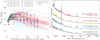 |
Fig. B.1 Left: Swift-UVOT UVW2 band light curves from Jacobson-Galán et al. (2024b) for SNe II with (solid red lines) and without (dashed blue lines) early-time IIn-like spectral features. Model light curves are shown for mass-loss rates of 0.1 M⊙yr−1 (circles), 0.01 M⊙ yr−1 (stars), and 0.001 M⊙yr−1 (squares). Varying model CSM radii of 2, 6, and 10 ×1014 cm shown as grey, magenta and cyan symbols. Low kinetic energy model (Ekin = 6 × 1050 erg) with varying mass-loss rates are shown as orange symbols. Right: Optical spectra of SNe 2013fs (red), 2020pni (yellow), 2022pgf (blue) and 2018zd (green) from the SN II sample compiled by Jacobson-Galán et al. (2024b) compared to best-match spectra (black) from current model grid at a similar phase. All models shown have consistent IIn timescales to the SNe being compared. |
Appendix C The luminosity offset between HERACLES and CMFGEN
Our methodology for the modeling of SN ejecta that interact with the CSM is to postprocess the results from radiation-hydrodynamics simulations (e.g., with HERACLES) with NLTE radiative transfer (e.g., with CMFGEN). The goal is to combine the distinct assets of each code to handle the complicated dynamics of these configurations while providing detailed observables that can be confronted to observations. In past works, we provided direct comparison to specific SNe of both light curves and spectra (i.e., the interacting SN 2010jl, Dessart et al. 2015; SN 1998S or SN 1994W, Dessart et al. 2016) or model grids falling in the parameter space of certain types of SNe (e.g., Type II SNe exploding within confined CSM, Dessart et al. 2017), and including polarization (e.g., SN 2010jl, Dessart et al. 2015; SN 1998S, Dessart et al. 2025). With this method, we made a critical improvement over our first effort at modeling an interacting SN in which we ignored the hydrodynamics and treated the radiative transfer for an idealized, simplistic configuration limited to the photospheric region (Dessart et al. 2009).
The crux of the method, which was laid out in Dessart et al. (2015) is to import the hydrodynamical variables from HERACLES into CMFGEN and solve for the radiative transfer by fixing the temperature of the gas (i.e., the electron temperature). We justified this choice by arguing that in interacting SNe the shock is the main power source (combined with weaker power diffusing from deeper layers, either from previous shock passage or radioactive decay) such that the temperature structure has a complicated profile with multiple peaks, with radiative energy diffusing inward and outward from those peaks etc. Hence, the configuration is time dependent and out of radiative equilibrium. In our approach, we also imported into CMFGEN the complicated velocity structure, with distinct regions being accelerated or decelerated, possibly with multiple shocks. To handle this essential feature, a new solver was designed in CMFGEN that no longer requires homologous expansion but instead can treat nonmonotonic flows (although in expansion, i.e., V > 0). The downside is the use of the Sobolev approximation rather than the more accurate blanketing mode (Hillier & Miller 1998), but this is worthwhile since CMFGEN can then make detailed predictions for the line profile morphology and its evolution in time, in particular concerning the relative importance of electron scattering versus Doppler broadening. These signatures are essential for characterizing the fundamental properties of SNe with CSM interaction.
Times over which specific optical electron-scattering broadened emission lines are present in the model spectra computed for our 27 ejecta and CSM configurations characterized by different values of Ekin, Ṁ, and Rcsm.
One limitation of this approach is that the temperature imported from HERACLES into CMFGEN leads to a lower luminosity prediction in CMFGEN, which arises from the influence of lines, in particular in the UV. Some level of disagreement is expected since the two codes have completely different approaches for solving the radiative transfer, with a treatment in LTE in HERACLES and in NLTE in CMFGEN. And the level of complexity of each code is totally different: HERACLES does this calculation about a million times in the course of a simulation covering the shock breakout phase out to 15 d, taking about five hours with 128 processors (MPI parallelization). In contrast, each snapshot (i.e., one time) simulated with CMFGEN takes about 24 hours with 16 processors (OpenMp parallelization).
There are only few comparisons of radiative-transfer codes in the literature. In Blondin et al. (2022), different codes were tested for Type Ia SN ejecta conditions and compared in their predictions for the light curve, ejecta temperature, ionization etc. Although applied to a different SN type, this comparison is very informative. Indeed, despite the simplicity of the configuration (i.e., smooth homologous flow, radioactive decay power source only etc), the codes differed in their predictions, and in particular did not yield the same temperature (see their Fig. 7). In other words, if we were to feed into these various codes the same temperature structure at a given time and recomputed the radiative transfer with that temperature fixed, each code would predict a different luminosity and a different spectrum, even in this idealized configuration.
Dessart et al. (2025) also compared the prediction of the blanketed solver and the Sobolev, nonmonotonic solver in CMFGEN for a configuration suitable for the interacting SN 1998S. The calculations were performed at times when the shock was still deep in the CSM so that most of the CSM was unshocked and optically thick. In this situation, one may in the blanketed solver assume homologous expansion by resetting the velocity so that the whole configuration is at the same age of Rphot/Vphot (for additional details, see Appendix A of Dessart et al. 2025). We then found that the blanketed solver yielded a similar optical spectrum to the nonmonotic solver, with a better agreement of the blanketed solver for the N III-C III blend at 4600 Å in SN 1998S. The blanketed solver also yielded a 40% higher luminosity than the nonmonotonic solver (with the offset arising primarily in the UV where the bulk of the escaping radiation falls), although both used the same temperature (which was held fixed). Again, this is not surprising given the simplified treatment of lines in the Sobolev approximation.
This implies that the luminosity obtained by CMFGEN based on the HERACLES temperature is not very accurate, with a typical offset of ≲ 80%. This is representative only since the offset is often smaller (see other examples in Fig. C.1), and comes as well with a time offset. Indeed, in those luminosity comparisons, we have to shift the HERACLES light curve in time because of the light-travel time of 1.5 d to the outer grid boundary (this is also augmented by an additional offset reflecting the diffusion time through the CSM). This arises because HERACLES is time dependent (and uses a eulerian grid) whereas the present CMFGEN solver is steady state (and lagrangian). These light-curve comparisons should thus be considered with these limitations in mind – we are not seeking nor claiming 1% accuracy but instead aim at developing a conceptual understanding of these complicated ejecta configurations. But one should also bear in mind that all radiation-hydrodynamics codes in the SN community assume LTE for the gas and have limitations (often aggravated by the use of grey transport and flux-limited diffusion). Importantly, none of these other works provide detailed spectroscopic information of the kind delivered by our method.
 |
Fig. C.1 Same as Fig. 4 but for the models ekin1p2_mdot1em6 (left), ekin1p2_mdot0p01_rcsm2e14 (middle) and ekin1p2_mdot0p01_rcsm1e15 (right). |
In the context of blackbody radiation in which the luminosity goes as the fourth power of the temperature, an 80% offset in luminosity corresponds to a 15% offset in temperature. This is rather small given the large differences in luminosity for our model set, both in terms of time (e.g., rise and decline time scales) and magnitude (factor of 10–100 in bolometric luminosities at a given post-breakout time). We show in Fig. C.2 the counterpart of Fig. 3 for the photospheric temperature versus time for the whole model set, including the cases without CSM (this photospheric temperature is a proxy for the complicated temperature profile, which cannot easily be shown for all simulations and all times). Evidently, the variation between these different curves far exceeds a 15% offset responsible for the luminosity offset reported above. But it also shows that importing this complex variation into CMFGEN (in reality importing the whole temperature profile) is critical to capture the associated variations in ionization. Indeed, the differences in line profile morphology or species ionization are driven by temperature differences of more than a factor of ten, encoded as well in a temporal variation that differs strongly between CSM configurations.
We believe that our approach is still appropriate given the challenges. Indeed, the complex temperature structure resulting from the presence of a shock is critical. Iterating between HERACLES and CMFGEN would not help since the two codes differ (i.e., LTE vs NLTE for the gas) – the iteration would never converge. The computational burden is also unmanageable because HERACLES requires up to a million timesteps for a full calculation (the explicit solver is used because of the presence of a strong shock – the implicit solver is not stable enough for the task). Iterating with CMFGEN, which takes about a day for one calculation, is unthinkable.
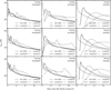 |
Fig. C.2 Counterpart of Fig. 3 showing the evolution of the photospheric temperature obtained with the multigroup radiation-hydrodynamics code HERACLES for our model set. The x-axis origin corresponds to the time when the shock crossed R∗. |
But solutions have been found for some CSM configurations. Indeed, if the CSM density is low (i.e., the CSM is optically thin), one may ignore the dynamical effects of the interaction with the CSM with the exception of the power released at the shock. Assuming homologous expansion holds (which it approximately does), the full-blanketed CMFGEN solver can then be used to evolve the ejecta time-dependently to late times, even out to several years (Dessart & Hillier 2022; Dessart et al. 2023), with compelling results when confronted to observations like SN 2023ixf (Bostroem et al. 2024; Kumar et al. 2025; Jacobson-Galán et al. 2025; Zheng et al. 2025). A similar approach was also used for the modeling of SNe Ibn and yielded a compelling match to their unique post-peak spectral characteristics (Dessart et al. 2022). This method, however, does not work for dense, extended, optically thick CSM affecting both the diffusion of radiation and the ejecta dynamics.
Despite this shortcoming, the predictions of HERACLES and CMFGEN in this combination and approximations are robust for the spectral evolution (ionization of species, profile morphology, radiative acceleration of the unshocked CSM etc). The dynamics is sound, as well as the predictions of HERACLES for the bolometric light curve. As discussed in Sect. 4, we expect the magnitudes predicted by CMFGEN to be underestimated by 0.5–1.0 mag, and this primarily in the UV where the bulk of the flux is radiated at early times. HERACLES is run with just eight energy groups in order to capture the large opacity differences between the various photoionization jumps of hydrogen (see discussion in Dessart et al. 2015). Running with more energy groups was tested back in 2015 but this was found to make little difference, the critical benefit being to avoid the grey approximation (i.e., a single-group calculation) because any opacity mean may vastly underestimate the opacity in some spectral regions (e.g., the opacity in the Lyman continuum for a cold gas). The rational was instead to limit the HERACLES simulations to a small number of energy groups, but then postprocess the results with CMFGEN, which solves the radiative transfer at 105–106 frequency points from the extreme UV to the infrared.
Appendix D Grid resolution
Our work employs a combination of four different codes and thus, as discussed in the preceding section, there are inevitable diffi-culties when importing the results of one code into another. The transition from MESA to V1D is straightforward because both codes are lagrangian. The explosion in V1D is treated with a thermal bomb and treated essentially with pure hydrodynamics until the shock approaches the progenitor surface (typically within 100 R⊙ of R∗). That is, the radiation is trapped behind the shock and there is no diffusion of radiation at the time of remapping into HERACLES. In this remapping, we take the structure of the V1D ejecta up to a radius just external to the shock, paste the outer structure from the progenitor in MESA, and augment it with a CSM configuration that extends out to 4 × 1015 cm (see Fig. 1). Finally, when postprocessing the HERACLES simulations with CMFGEN, we limit the whole configuration to the region located between an electron-scattering optical depth of about 10−4 up to about 50 – most of the emission arises from regions between optical depths of 0.1 and 10.
The number of grid points differs vastly between codes. In the MESA and V1D calculations, which are lagrangian, we used 1000–2000 points for the whole star, with a mass resolution covering from about 10−6 to 10−2 M⊙. In all HERACLES calculations, we used a total of 14336 grid points (i.e., a multiple of 128) which are arranged linearly from 1013 (regions near and below this radius have no importance over the 15 d of physical time covered in the present work) up to 5 × 1014 cm, and transitions smoothly (i.e., the radial increment is equal on each side of the transition) to a logarithmic spacing out to the maximum radius at 4 × 1015 cm. This ensures high resolution near and beyond R∗ where the density drops steeply. Finally, we use 80–100 grid points in the CMFGEN calculations but the gridding is adaptive to capture the jumps in density, temperature, and allocate 5–7 depth points per optical-depth decade (see, for example, Fig. A.1 in Dessart et al. 2025). This gridding is critical to obtain convergence of the radiative transfer. This choice of gridding was the result of convergence tests done in 2017 to improve the earlier, lower-resolution calculations presented in Dessart et al. (2015).
There is mild shock smoothing in V1D because the code uses artificial viscosity (see, e.g., the simulations shown in Paxton et al. 2015 and more recently in Roussel-Hard et al. 2025) but no additional smearing is introduced when remapping into HERACLES given the huge resolution employed. The adaptive gridding on an optical-depth scale in CMFGEN ensures a proper resolution on the scale that truly matters for radiative transfer, typically delivering a much higher resolution than in radiation-hydrodynamics codes, whether they grid in mass or in radius.
Seeking for the highest resolution is meritorious as far as internal consistency is concerned, in particular when going from one code to another. However, there is also a conceptual danger in doing this since one then resolves accurately 1D structures that typically do not exist in 3D or in nature. The dense shell created in the interaction of ejecta with the CSM is accurately compressed into a thin layer in our 1D HERACLES simulations, and the more so the higher the resolution. But this structure is an artifact of 1D. The dense shell should break-up in 3D. Similarly, shock breakout would appear very differently in a 3D progenitor, 3D explosion, 3D CSM (see, for example, Goldberg et al. 2022b). The approximation of spherical symmetry is likely the largest source of uncertainty in our work (i.e., not a numerical uncertainty but one related to the overall realism when comparing to observations), even though we employ a much higher resolution than possible in 3D. For example, our 1D HERACLES simulations employ 14336 radial grid points whereas the 3D simulations of Goldberg et al. (2022b) have only ∼400 radial grid points.
Appendix E Additional illustrations
In this section we present additional illustrations to complement the main text. Figure E.1 illustrates the V-band light curve for our model set as computed with CMFGEN (see Fig. 5 for the UVW2-band countpart). We also show in Fig. E.2 the simultaneous evolution of the Hα region and the structure of the spectrum formation region in model ekin1p2_mdot0p1_rcsm2e14. Finally, Fig. E.3 shows the step-by-step evolution of the rectified spectra for model ekin1p2_mdot0p01_rcsm6e14 (all computed epochs are shown).
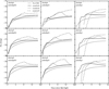 |
Fig. E.1 Same as Fig. 5 but now showing the V-band light curves computed with CMFGEN for our model set. |
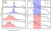 |
Fig. E.2 Same as Fig. 6 but for model ekin1p2_mdot0p1_rcsm2e14. All contributing lines are included in this figure, including He I at 6678.15 and He II at 6560.09 Å (this line dominates the emission seen at 2.0 d and remains a strong contributor at 2.5 and 3.0 d). This configuration with a more compact and denser CSM fosters a strong radiative acceleration of the unshocked CSM (causing the disappearance of the SN shock at all epochs shown), visible in the blue-shifted emission for the last two epochs (i.e., two bottom rows). |
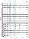 |
Fig. E.3 Evolution of the total flux normalized to the continuum flux for model ekin1p2_mdot0p01_rcsm6e14. |
All Tables
Summary of the CSM properties we adopted as initial conditions for our model grid.
Light-curve and ejecta properties from the HERACLES simulations for our model grid.
Times over which specific optical electron-scattering broadened emission lines are present in the model spectra computed for our 27 ejecta and CSM configurations characterized by different values of Ekin, Ṁ, and Rcsm.
All Figures
|
Fig. 1 Preshock breakout density profiles used as initial conditions for the radiation-hydrodynamics calculations. The model is for a progenitor star of 15 M⊙ initially and evolved at solar metallicity, which after explosion yielded an ejecta with a kinetic energy of 1.2 × 1051 erg. The CSM configurations are characterized by a different extent (RCSM values of 2, 6, and 10 × 1014 cm, indicated by solid, dotted, and dashed lines) and density (Ṁ values of 0.1, 0.01, and 0.001 M⊙yr−1). The same velocity law is used in all cases. For details, see Sect. 2. |
| In the text | |
|
Fig. 2 Results from the radiation-hydrodynamics calculations for our sample of 27 ejecta and CSM configurations. Left: peak luminosity vs. rise time to peak. Middle: Time-integrated bolometric luminosity vs. maximum ejecta velocity, both evaluated at 15 d. Right: CDS velocity vs. CDS mass at 15 d. The colors signify different model kinetic energies, the symbols show the mass-loss rate, and the filling style shows the CSM extent. These indications, which apply to all panels, are given separately, one panel at a time for better visibility. For comparison, we also show the results for the three No-CSM cases (empty diamonds). The interaction phase is not concluded in models with a high CSM mass and extent, so the values are not yet converged at 15 d in these cases. |
| In the text | |
|
Fig. 3 Bolometric light curves calculated with the multigroup radiation-hydrodynamics code HERACLES and tiled according to the model ejecta kinetic energy (one value per row), CSM density (one value of M˙ per column), and CSM extent (three values per panel, with the No-CSM counterpart shown as a dotted line). The x-axis origin is chosen to be when each model first brightens to a luminosity of 1040 erg s−1, as recorded at the outer grid boundary. |
| In the text | |
|
Fig. 4 Comparison between the HERACLES and CMFGEN bolometric light curves for model ekin1p2_mdot0p01_rcsm6e14. The HERACLES light curve has been shifted in time to correct for the light-travel time to the outer grid boundary. |
| In the text | |
|
Fig. 5 Same as Fig. 3, but now showing the UVW2-band light curves computed with CMFGEN for our model set. |
| In the text | |
|
Fig. 6 Correspondence between the Hα evolution (left column; only H I lines are included in the displayed range) and the dynamical properties in the spectrum formation region (right column) for model ekin1p2_mdot0p01_rcsm6e14. The shading differentiates emission from the unshocked CSM (blue) and the shocked material (red), which corresponds here to the dense shell. The spectrum forms preferentially over regions in which log τ is between −1 and 1, except for the narrow-line core arising from regions at log τ of about −2. Here, V8 refers to the velocity in units of 108 cm s−1 and T4 is the gas (or electron) temperature in units of 104 K (log ρ is the base-10 logarithm of the density, shown with an additive constant for better visibility). |
| In the text | |
|
Fig. 7 Spectral morphology during the IIn phase that results from a range of ionization of the unshocked CSM, from cool weakly ionized conditions at the top to hot and highly ionized conditions at the bottom. The models shown here differ in ejecta and CSM configuration and in post-breakout time. In all cases, He II 6560.1 Å is a contaminant to the Hα emission. |
| In the text | |
|
Fig. 8 Comparison of the spectral evolution of model ekin1p2 with a CSM (left; case mdot0p01 and rcsm6e14) and without CSM (right). The rest wavelength of the main lines is indicated and is also color-coded to differentiate different species. The lines that are affected by Doppler broadening exhibit a strong blueshift and can primarily appear in absorption (later epochs in the CSM case during the CDS phase) or primarily in emission (No-CSM case). See Sect. 5.3 for a discussion. |
| In the text | |
|
Fig. B.1 Left: Swift-UVOT UVW2 band light curves from Jacobson-Galán et al. (2024b) for SNe II with (solid red lines) and without (dashed blue lines) early-time IIn-like spectral features. Model light curves are shown for mass-loss rates of 0.1 M⊙yr−1 (circles), 0.01 M⊙ yr−1 (stars), and 0.001 M⊙yr−1 (squares). Varying model CSM radii of 2, 6, and 10 ×1014 cm shown as grey, magenta and cyan symbols. Low kinetic energy model (Ekin = 6 × 1050 erg) with varying mass-loss rates are shown as orange symbols. Right: Optical spectra of SNe 2013fs (red), 2020pni (yellow), 2022pgf (blue) and 2018zd (green) from the SN II sample compiled by Jacobson-Galán et al. (2024b) compared to best-match spectra (black) from current model grid at a similar phase. All models shown have consistent IIn timescales to the SNe being compared. |
| In the text | |
|
Fig. C.1 Same as Fig. 4 but for the models ekin1p2_mdot1em6 (left), ekin1p2_mdot0p01_rcsm2e14 (middle) and ekin1p2_mdot0p01_rcsm1e15 (right). |
| In the text | |
|
Fig. C.2 Counterpart of Fig. 3 showing the evolution of the photospheric temperature obtained with the multigroup radiation-hydrodynamics code HERACLES for our model set. The x-axis origin corresponds to the time when the shock crossed R∗. |
| In the text | |
|
Fig. E.1 Same as Fig. 5 but now showing the V-band light curves computed with CMFGEN for our model set. |
| In the text | |
|
Fig. E.2 Same as Fig. 6 but for model ekin1p2_mdot0p1_rcsm2e14. All contributing lines are included in this figure, including He I at 6678.15 and He II at 6560.09 Å (this line dominates the emission seen at 2.0 d and remains a strong contributor at 2.5 and 3.0 d). This configuration with a more compact and denser CSM fosters a strong radiative acceleration of the unshocked CSM (causing the disappearance of the SN shock at all epochs shown), visible in the blue-shifted emission for the last two epochs (i.e., two bottom rows). |
| In the text | |
|
Fig. E.3 Evolution of the total flux normalized to the continuum flux for model ekin1p2_mdot0p01_rcsm6e14. |
| In the text | |
Current usage metrics show cumulative count of Article Views (full-text article views including HTML views, PDF and ePub downloads, according to the available data) and Abstracts Views on Vision4Press platform.
Data correspond to usage on the plateform after 2015. The current usage metrics is available 48-96 hours after online publication and is updated daily on week days.
Initial download of the metrics may take a while.