| Issue |
A&A
Volume 707, March 2026
|
|
|---|---|---|
| Article Number | A253 | |
| Number of page(s) | 20 | |
| Section | Stellar atmospheres | |
| DOI | https://doi.org/10.1051/0004-6361/202557856 | |
| Published online | 24 March 2026 | |
X-Shooting ULLYSES: Massive stars at low metallicity
XIV. Properties of SMC late-O and B supergiants reveal the metallicity dependence of winds in the Magellanic Clouds
1
Astrophysics Research Cluster, School of Mathematical and Physical Sciences, University of Sheffield,
Hicks Building, Hounsfield Road,
Sheffield
S3 7RH,
UK
2
School of Chemical, Materials and Biological Engineering, University of Sheffield,
Sir Robert Hadfield Building, Mappin Street,
Sheffield
S1 3JD,
UK
3
Institute of Astronomy,
KU Leuven, Celestijnenlaan 200D,
3001
Leuven,
Belgium
4
Departamento de Astrofísica, Centro de Astrobiología, (CSIC-INTA),
Ctra. Torrejón a Ajalvir, km 4,
28850
Torrejón de Ardoz, Madrid,
Spain
5
Armagh Observatory and Planetarium,
College Hill,
Armagh
BT61 9DG,
UK
6
Zentrum für Astronomie der Universität Heidelberg, Astronomisches Rechen-Institut,
Mönchhofstr. 12–14,
69120
Heidelberg,
Germany
7
Interdisziplinäres Zentrum für Wissenschaftliches Rechnen, Universität Heidelberg,
Im Neuenheimer Feld 225,
69120
Heidelberg,
Germany
8
Institut für Physik und Astronomie, Universität Potsdam,
Karl-Liebknecht-Str 24/25,
14476
Potsdam,
Germany
9
Lennard-Jones Laboratories, Keele University
ST5 5BG,
UK
10
Faculty of Physics, University of Duisburg-Essen,
Lotharstraße 1,
47057
Duisburg,
Germany
★ Corresponding author: This email address is being protected from spambots. You need JavaScript enabled to view it.
Received:
27
October
2025
Accepted:
28
January
2026
Abstract
Context. Hot massive stars lose mass through radiation-driven winds, producing significant chemical, radiative, and mechanical feedback in the surrounding environment. The properties of these winds play a crucial role in determining the star’s evolutionary path. Considering the physics of radiation-driven winds, the wind properties should depend on the metal content of the stellar atmosphere. Therefore, studying the wind properties of massive stars in different metallicities (Z) provides a sanity check on prescriptions that are widely used in evolutionary calculations.
Aims. We first aim to obtain the stellar and wind properties of a sample of late-O and B supergiants in the Small Magellanic Cloud (SMC). Using these properties, we aim to quantify the dependence of wind properties on metallicity by comparing them with those of a Large Magellanic Cloud (LMC) counterpart study, which has a similar sample and data, and employed the same modelling techniques used in this study.
Methods. Spectroscopic modelling of UV and optical data from ULLYSES and XShootU was performed using the radiative transfer code CMFGEN. We also employed an updated Bayesian inference method similar to BONNSAI to explore the evolutionary history of our sample.
Results. We derived the stellar and wind properties of 20 late-O and B supergiants. We derived the following metallicity-dependent recipe for wind momentum: log Dmom = (1.64 − 0.75 log Z/Z⊙) log (Lbol/106 L⊙) + 1.38 log Z/Z⊙ + 29.17, which is applicable for 5.4 ≤ log Lbol/L⊙ ≤ 6.1 and 14 ≤ Teff/kK ≤ 32.
Conclusions. We find a significant dependence of the wind momentum on the metallicity, which is largely due to the mass-loss rates. We do not find any evidence of a discontinuity in either the mass-loss rate or the ratio of the terminal wind velocity to the escape velocity, v∞/vesc, between 25 and 21 kK, which could be attributed to the bi-stability jump, although when taking into account the effect of luminosity in the transformed mass-loss rate, the behaviour appears to be different. Stellar parameters are consistent across different methods and radiative transfer codes, whereas mass-loss rates differ significantly with our values being generally lower. We find a discrepancy between the evolutionary and spectroscopic masses in 40% of our sample, with the evolutionary mass usually being systematically higher. The mass-loss rates of blue supergiants are far too low to strip the stellar envelope and the subsequent formation of classical Wolf-Rayet (WR) stars, leading to the conclusion that luminous blue variable eruptions or binary interactions are necessary to explain characteristics of the WR population in the SMC.
Key words: stars: atmospheres / stars: early-type / stars: massive / stars: mass-loss / supergiants / stars: winds, outflows
© The Authors 2026
 Open Access article, published by EDP Sciences, under the terms of the Creative Commons Attribution License (https://creativecommons.org/licenses/by/4.0), which permits unrestricted use, distribution, and reproduction in any medium, provided the original work is properly cited.
This article is published in open access under the Subscribe to Open model. This email address is being protected from spambots. You need JavaScript enabled to view it. to support open access publication.
1 Introduction
Massive stars (M > 8 M⊙) possess strong outflows of material, which form due to the immense radiative pressure overtaking the force of gravity at the outer layers of the star. This allows the star’s atmosphere to expand beyond the boundaries of the photosphere. The properties of these outflows are strongly correlated to the ratio of luminosity to mass of the star (Eddington 1926). To overcome gravity, the acceleration due to free electrons has to be combined with so-called ‘line-driving’, i.e. momentum transfer from radiation absorbed (and re-emitted) in spectral lines (Lucy & Solomon 1970; Castor et al. 1975). This means that the momentum driving the winds of massive stars is transferred via spectral lines. This leads to the conclusion that the chemical content of the star, or the metallicity (Z), plays an important role in determining the properties of the winds (Abbott 1982). This is particularly true for metals, and especially iron-like species, which account for the majority of line driving. This is due to their complex atomic structure and the large number of line transitions in their ions.
The theory of line-driven wind and its implications for the Z dependence of wind properties have been studied in the literature. It is taken into account in the various numerical mass-loss recipes (e.g. Vink et al. 1999, 2001; Krtička et al. 2021). The Z dependence of mass-loss and wind velocity has also been well established observationally (e.g. Kudritzki et al. 1987; Prinja & Crowther 1998; Mokiem et al. 2007; Ramachandran et al. 2019; Hawcroft et al. 2024b). Nevertheless, there is a persistent discrepancy between the Z dependence that is predicted in theory and what is empirically derived from observations of blue supergiants in low-Z environments (Krtička et al. 2024).
The effects of Z extend beyond the academic interest in the wind properties of massive stars. Mass loss in massive stars is one of the factors that determines the evolutionary path of the star, including whether it is fated to explode in a type of core-collapse supernova (ccSNe II/Ib/Ic) and leave behind a black hole (BH) or a neutron star (NS) remnant (Smartt 2009), or whether it would experience direct collapse into a BH in a failed-nova scenario (for a review of the effects of mass-loss on the evolution of massive stars, see e.g. Smith 2014).
The winds of massive stars also play an important role in the chemical evolution of their host galaxies by enriching the interstellar medium (ISM) with heavy elements that are synthesised in their interiors and are transported to the surface of the star via efficient internal mixing processes (Langer 2012). The mass ejected via stellar winds propagates through the ISM at supersonic speeds, leading to strong mechanical feedback to the surroundings of massive stars. This, in addition to the enrichment of the ISM in heavy elements, leads to an increase in its opacity, affecting the star formation rate in the host galaxy (for a general review on massive star feedback see e.g. Geen et al. 2023).
Due to the abundant metal lines in B-type supergiants, they have been used to constrain heavy metal content in extragalactic environments (Urbaneja et al. 2005a,b; Trundle et al. 2004; Trundle & Lennon 2005; Bresolin et al. 2022). They have also been successfully used as distance indicators in external galaxies due to their high visual brightness (Kudritzki et al. 2003, 2024).
This study was made possible by the advent of the Hubble Ultra-violet Legacy Library of Young Stars as Essential Standards (HST ULLYSES, Roman-Duval et al. 2025). The HST ULLYSES programme dedicated 500 orbits to obtain high-resolution UV spectra of OB stars in low-Z environments, mainly the Large Magellanic Cloud (LMC) and Small Magellanic Cloud (SMC). The UV range is critical for determining the properties of the wind, but it lacks information about the underlying photosphere. For a fuller picture of the stellar and wind properties, we made use of the XShooting/ULLYSES optical spectroscopic legacy library (XShootU, Sana et al. 2024).
Recent efforts have been made by Marcolino et al. (2022), Backs et al. (2024), and Pauli et al. (2025) to constrain the Z dependence of wind properties and to produce empirical recipes for mass loss and wind momentum. These recipes, although very insightful, suffer from different issues. In particular, these recipes are produced using assumptions inferred from numerical recipes (Leitherer et al. 1992; Vink et al. 2001; Krtička et al. 2021; Björklund et al. 2023). Furthermore, luminosity classes are not taken into account in these recipes. Lastly, empirical recipes usually use results from the literature, which use different atmosphere codes and various datasets, some UV and optical, and some only optical, subjecting the derived parameters to large variance (Sander et al. 2024).
The present study may be viewed as the second in a series of papers, following Alkousa et al. (2025, henceforth Paper XIII), in which a sample of LMC late-O and B supergiants was analysed. In the present study, we expand our analysis of OB stars to the SMC. We aim to quantify the effect of Z on the properties of the wind. We do not aim to produce a full empirical recipe dependent on Z of mass loss, as doing this without forcing any assumptions from numerical simulations would require another Z environment, such as the Milky Way (MW), which we aim to undertake in a future study.
The XShootU and ULLYSES datasets have been used in recent studies of OB supergiants in the SMC, employing various radiative transfer codes and fitting techniques for different purposes. We compare our derived photospheric and wind parameters to those obtained by Bestenlehner et al. (2025), Backs et al. (2024), and Bernini-Peron et al. (2024) in Appendix F.
In Section 2, we present the dataset that was used in this study, our sample, and our selection criteria. In Section 3, we give a summary of our methodology, which was presented in Paper XIII in thorough detail. In Section 4, we introduce the results of our analysis. In Section 5, we discuss the implications of our results, including the effects of Z and the bi-stability jump.
2 Observations
In Table 1, we present the stars in our sample, along with their classification, which was adopted from Bestenlehner et al. (2025). In this table, we also include the telescope, instrument, and wavelength coverage available for each star.
This sample was selected in such a way that it would cover a spectral range similar to that of Paper XIII. We cover a wide range of spectral classes, from O9 to B8, which includes the region of the theorised bi-stability jump. We attempted to include more than one star per spectral class, ideally with different luminosity classifications (Ia+, Ia, Iab, Ib). This allowed us to explore the Z dependence of wind properties while avoiding selection bias, which we discussed in Paper XIII when contrasting our results for the LMC sample with the results of Bernini-Peron et al. (2024) in the SMC, whose sample was made up almost exclusively of Ia supergiants. We have ten stars in common with Bernini-Peron et al. (2024), who include eight stars that are not covered in our study, while we include ten stars not covered in Bernini-Peron et al. (2024). That makes the two studies complementary, although with slightly varying modelling techniques (X-rays and micro-turbulence), and an excellent opportunity to compare the results in our overlapping samples.
A subset of our sample has been included in the BLOeM survey (Shenar et al. 2024). Britavskiy et al. (2025) did not find evidence of significant radial velocity shifts across nine epochs of this subset, indicating that these stars are apparently single. They report that AzV 242 (BLOeM 4-078) and AzV 96 (BLOeM 8-008) show intrinsic line profile variability, with the possibility that AzV 242 is an SB1 spectroscopic binary.
List of the stars included in our analysis and the respective wavelength coverage.
2.1 ULLYSES
The ULLYSES programme (Roman-Duval et al. 2025) made use of two instruments aboard HST ; namely, the Cosmic Origins Spectrograph (COS, Green et al. 2012) in the G130M/1291, G160M/1611, and G185M/1953 wavelength settings, achieving a minimum spectral resolving power of R ≈ 12 000, R ≈ 13 000, and R ≈ 16 000, respectively, and the Space Telescope Imag ing Spectrograph (STIS, Woodgate et al. 1998) E140M/1425 (R ≈ 46 000), and E230M/1978 (R ≈ 30 000) gratings in the far-and near-UV. New COS and STIS spectra were obtained for a subset of our targets between July 2020 and Sept 2022, and were combined with archival HST spectra drawn from GO 7437 (PI: Lennon), GO 9116 (PI: Lennon), GO 12581 (PI: Roman-Duval), GO 13778 (PI: Jenkins), and GO 15837 (PI: Oskinova) obtained between Oct 2001 and Jun 2020. A subset of HST spectra have previously been presented by Walborn et al. (2000) and Evans et al. (2004).
Archival spectra from the Far Ultra-violet Spectroscopic Explorer (FUSE, Moos et al. 2000) cover the wavelength range of ≈900–1160 Å and uniformly involve the LWRS (30′′ × 30′′) aperture for our sample, providing R ≈ 15 000. These are drawn from various Principal Investigator Team and Guest Investigator programmes obtained between May 2000 and July 2003. FUSE spectroscopy of a subset of the current sample has previously been presented by Walborn et al. (2002). We note that AzV 327 lies in a crowded region, such that other sources, including [M2002] SMC 55495, contribute to the FUSE spectrum (Danforth et al. 2002).
2.2 XShootU
ULLYSES targets were observed using the X-shooter instrument (Vernet et al. 2011), which is mounted on the Very Large Telescope (VLT). This slit-fed spectrograph (11′′ slit length) provides simultaneous coverage of the wavelength region between 3000–10 200 Å, across two arms: UVB (3000 ≤ λ ≤ 5600 Å) and VIS (5600 ≤ λ ≤ 10 200 Å). The observations were carried out between October and December 2020 with a slit width 0.8′′ for the UBV arm, achieving R ≈ 6700, and 0.7′′ for the VIS arm, with R ≈ 11 400 (Vink et al. 2023). All science-ready optical spectra used in this study were combined, flux-calibrated, corrected for telluric contamination, and normalised by Sana et al. (2024, DR1), except for archival X-shooter spectroscopy of AzV 187 from November 2013, which we normalised using a higher-order polynomial fit of points selected around regions of clean continuum.
2.3 Photometry
The photometric magnitudes used in this study were taken from the compilation in Vink et al. (2023) to derive the bolometric luminosities by fitting the SED spectral energy distribution. The UBV photometry was taken from Ardeberg & Maurice (1977), Azzopardi et al. (1975), Ardeberg (1980), and Massey (2002), and the JKs photometry was drawn from the VISTA near-infrared YJKS survey of the Magellanic System (VMC, Cioni et al. 2011), with H-band photometry taken from the Two Micron All Sky Survey (2MASS, Cutri et al. 2003; Skrutskie et al. 2006; Cutri et al. 2012).
2.4 MIKE spectroscopy
High-resolution optical spectroscopy used to extract the rotational properties of slow rotators was collected between Decem-ber 2021 and December 2022 using the Magellan Inamori Kyocera Echelle (MIKE) spectrograph mounted on the Magellan Clay 6.5 m Telescope, covering the wavelengths 3350 to 5000 Å in the blue arm and 4900 to 9500 Å in the red arm, achieving R ≈ 35 000–40 000 (Crowther 2024).
3 Methods
In this section, we present a summary of the modelling and fitting techniques used in our analysis. In the present study, we employ the same strategies as in Paper XIII. Therefore, for a comprehensive and detailed description of our methodology, we refer the reader to Paper XIII.
3.1 Model atmosphere and grid
We employed the 1D radiative transfer code CMFGEN (Hillier 1990; Hillier & Miller 1998), which solves the radiative transfer equations in spherical symmetry in non-local thermodynamic equilibrium (non-LTE), taking into account the effects of mass loss under the assumption of purely radial outflows. CMFGEN also accounts for the effects of extreme UV blanketing caused by millions of lines of iron-like species and other elements on populations and the ionisation structure in the wind. This is implemented using super-levels (Anderson 1985, 1989), which allow for the bundling of levels with similar energies and properties into a single or a super-level. This significantly reduces the number of statistical equilibrium equations that must be explicitly solved.
CMFGEN does not calculate the velocity stratification in the wind consistently with radiative acceleration, but rather superimposes a velocity law with a simple β parametrisation. Additionally, wind inhomogeneities are considered under the ‘optically thin clumping’ approximation, or micro-clumping, assuming that these optically thin clumps are smaller than the mean free path of the photons (Hillier 1996) and that the medium between the clumps is completely void of matter (Hillier 1997; Hillier & Miller 1999).
In Table 2, we present the properties of our grid. The effective temperature, Teff, surface gravities, log (g/cm s−2), and mass-loss rates,  , were refined starting from the preferred grid model. Other parameters, such as elemental abundances (ϵX = log X/H + 12), wind acceleration parameter, β, volume filling factor, fvol,∞, and terminal wind velocity, v∞, were fixed in the grid, but were later fine-tuned for each star. Stars that have Teff or log g values outside of the range covered by the grid were handled by building miniature grids and using those grids to fine-tune the model parameters.
The atomic model and data used in this study are identical to those shown in Table C.1 in Paper XIII. We included 14 species and 50 different ions. In cooler models (<25 kK), we omitted higher ionisation stages and included the lower ionisation stages. This is important for model convergence and for the iron forest in the UV spectra of B stars.
Also, similarly to Paper XIII, we excluded X-rays from our fitting procedure to guarantee a homogeneous analysis without variations in the techniques. X-rays, which were included in Bernini-Peron et al. (2024), increase the population of high ionisation stages (super-ionisation), affecting the strength of P Cygni resonance lines in the UV, such as N V λ1238, 1242, Si IVλλ1394, 1403, and C IV λλ1548, 1551. The super-ionisation comes at the expense of depopulating the lower ionisation stages, affecting lines of Al III and C ii.
In our grid, we choose a simple modified β velocity law that was introduced in Castor & Lamers (1979):
 (1)
(1)
where v∞ is the terminal wind velocity, v0 is the connection velocity, which is estimated as two-thirds the speed of sound ≈10 km s−1, and R∗ is the radius of the star, which is defined at the Rosseland optical depth τ = 100. The velocity adopted for each point on the grid was obtained via the Teff and Z-dependent empirical recipe from Hawcroft et al. (2024b):
![Mathematical equation: $\eqalign{& {v_\infty }\left( {{\rm{km}}{{\rm{s}}^{ - 1}}} \right) = \left[ {0.092( \pm 0.003){T_{{\rm{eff}}}}({\rm{K}})} \right. \cr & - 1040( \pm 100)]Z/Z_ \odot ^{(0.22 \pm 0.03)}, \cr}$](/articles/aa/full_html/2026/03/aa57856-25/aa57856-25-eq4.png) (2)
(2)
which was derived from Sobolev with exact integration (SEI) modelling of the P Cygni resonance doublet C iv λλ1548–1551 to measure the terminal wind velocity. We adopted Z = 0.2 Z⊙ in Equation (2) (Vink et al. 2023).
To account for wind inhomogeneity, we adopted an exponential clumping law of the form
 (3)
(3)
where fvol,∞ is the terminal volume-filling factor and vcl is the onset clumping velocity. We adopted the values fvol,∞ = 0.1 and β = 1 in the grid, both of which were later modified in the fine-tuning process to obtain satisfactory fits for the Hα and UV P Cygni lines.
The grid spans a range for the transformed radius, log Rt (Schmutz et al. 1989), of between 2.1 and 4.0 on a logarithmic scale, where  , with smaller values relating to denser winds. This log Rt range corresponds to a range of optical depth-invariant wind-strength parameters,
  (Puls et al. 1996), of −15.0 to −12.5, where larger values of log Q correspond to denser winds. We employed Rt to scale
  to the derived bolometric luminosity of the star.
CMFGEN SMC-metallicity grid parameters.
3.2 Fitting procedure and diagnostics
We first used the results of Bestenlehner et al. (2025) to pinpoint the closest fitting model on the grid in log Teff-log g-log  parameter space, after which we start the fine-tuning procedure. The analysis in Bestenlehner et al. (2025) is based on the model de-idealisation pipeline, which applies a minimisation and interpolation routine using a large grid of FASTWIND models (Puls et al. 2005; Rivero González et al. 2011). This allows for the estimation of stellar parameters and the mass-loss rates and model uncertainties using only optical spectroscopy (Bestenlehner et al. 2024).
Once we selected the nearest grid model, we started by fine-tuning the values of Teff, log g, and the helium abundance iteratively until a satisfactory fit was achieved. Then we iteratively fine-tuned log  , β, fvol,∞, and v∞ to fit Hα and the UV P Cygni lines. Finally, the CNO mass fractions were fine-tuned for each star.
Here, we give a summary of the fitting procedure. The approach for determining the goodness of the fit was ‘χ-by-eye’. For an extensive description of the fitting techniques, diagnostics, and uncertainty determination, we refer the reader to Section 3 of Paper XIII.
Effective temperature, Teff. We obtained the effective temperature from the principle of ionisation equilibrium. In O supergiants the primary Teff diagnostics are He i λ4471–He ii λ4542 (Martins 2011). For early and mid-B supergiants, we used ratios of adjacent ions of silicon as primary diagnostics (McErlean et al. 1999); namely, Si iv λλ4088–4116 versus Si III λλλ4553–4568– 4575 for B0 to B2 stars, and Si iii λλλ4553–4568–4575 versus Si ii λλ4128–4131 for B2.5–B3 stars. Note that in early B stars the Si iv λ4088.96 line is blended with O ii λ4089.29 (Hardorp & Scholz 1970; de Burgos et al. 2024b), so we ensured that this transition is accounted for in the adopted atomic model. For B8 supergiants, we used the ratio of He iλ4471 to Mg ii λ4481 to determine Teff.
Surface gravity log g. We determined the surface gravity by fitting the wings of Balmer lines, which are very sensitive to Stark broadening. The primary log g diagnostics for all stars in our sample are Hγ, Hη, and Hζ. These lines are relatively isolated – in contrast with Hδ – and are usually not contaminated by wind effects (Lennon et al. 1992).
Luminosity. To determine the bolometric luminosity, Lbol, of stars, we used the model fluxes (which were calculated for log Lmodel/L⊙ = 5.8). The reddening law from Gordon et al. (2003) was then applied to the model fluxes. We then fitted the relative extinction, RV, and other parameters that determine the shape of the UV extinction curve (Fitzpatrick & Massa 1990). Then the intrinsic colours were obtained (Bm, Vm, and K sm) by applying filter functions from PYPHOT (Fouesneau 2025) to the model SED using the Vega magnitude system photometric zero-point (for more details on PYPHOT, see Table 3 in Paper XIII). The colour excess E(B V) was calculated as (B − V) − (Bm − Vm). The model SED− was then scaled to match observations using a factor equal to the ratio of Ks fluxes  . The bolometric correction, BCV, was calculated as −2.5 log Lmodel + 4.74 − Vm. The final Lbol was calculated as
  , where AV = RV·E(B − V), and assuming a distance modulus of DM = 18.96 (corresponding to a distance d = 62 kpc) for the SMC (Scowcroft et al. 2016). In other relevant XShootU studies, a value of 18.98 for the distance modulus was adopted from Graczyk et al. (2020).
Helium mass fraction. We obtained the helium abundance by fitting He I and He II lines relative to hydrogen lines. The diagnostic lines used across the sample are He I λ4026, He I λ4471, and He I λ4922 for O and B supergiants, and He II λ4542 and He II λ5411 for O supergiants. We also used He I λ6678, He I λ7065, and He I λ7281 as a sanity check.
Wind density parameters. The wind density, ρ, is defined by v∞,  , fvol,∞, β, and vcl. The primary optical diagnostic line for
  and β is Hα (∝ ρ2). The UV unsaturated P Cygni profiles provide valuable information on wind inhomogeneities (Massa et al. 2008; Searle et al. 2008; Puls et al. 2008). The UV lines that we used to constrain
  and fvol,∞ are S ivλλ1063–73, C iiiλ1176, Si ivλλ1394–1403, C iv λλ1548–51, and Al iiiλλ1856–62. 3cl was adopted as two times the speed of sound of the model. v∞ was obtained from either (i) direct measurements of the black velocity, 3black (the velocity measured at the bluest extent of fully saturated P Cygni absorption (Prinja et al. 1990)), or (ii) as a fraction of vedge (the velocity measured at the point where the blue trough of the P Cygni profile intersects the local continuum (Beckman & Crivellari 1985)). We present the results of the velocity measurement in Table. E.1.
Line broadening parameters. Absorption lines are broadened by the effect of rotation (Slettebak 1956), photospheric macro-turbulence, vmac (Conti & Ebbets 1977; Simón-Díaz et al. 2010; Simón-Díaz & Herrero 2014), and micro-turbulence, vmic (McEr-lean et al. 1998). We fixed vmic = 20 km s−1 and vmic = 10 km s−1, and only determined the projected rotational velocity, vrot sin i, using metal lines. For O stars, our primary diagnostic is O iii λ5592. For early B stars, we used C iii λ4267 and Si iii λ4553. For mid- to late-B stars, we fitted the N ii λ3995 line and, as a sanity check, we used Si ii λ6347, the Mg ii λ4481 doublet, and C ii λ4267.
CNO abundances, ϵX. The abundances of carbon, nitrogen, and oxygen were constrained by fitting multiple optical absorption lines of each element. The selection of lines depends on the ion that dominates the photosphere in each spectral type. In Table D.1, we present our choice of diagnostic lines. The CNO abundances (among other metals) are arguably the most sensitive parameters to changes in photospheric micro-turbulent velocity, vmic (Urbaneja et al. 2005b). Fixing vmic in our analysis reduces the precision of our derived CNO abundances. This is due to the effect that changing the photospheric vmic has on the opacity, and therefore on the line strength of different components of multiplets (McErlean et al. 1998).
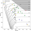 |
Fig. 1 Hertzsprung–Russell diagram for our sample. Overlaid in solid black lines are non-rotating SMC isochrones for different ages (≈0−10 Myr). Dashed black lines are the SMC rotating evolutionary tracks for stellar masses in the range of ≈10–60 M⊙ with a rotational velocity of 110 km s−1. Both the isochrones and evolutionary tracks are adopted from Brott et al. (2011). The shaded area is defined by the HD limit (Humphreys & Davidson 1979; Smith et al. 2004; Davies et al. 2018). |
4 Results
In this section, we present an overview of the results of our analysis. We compare our results with those from previous studies of SMC blue supergiants. In addition, we compare the derived wind parameters with predictions from numerical recipes. In Table A.1, we present the derived physical parameters and the inferred evolutionary masses and ages. In Appendix F, we compare our derived stellar and wind parameters to values from the literature. Comments on the spectral fitting quality are provided for each star individually in Appendix G. The SED fits, individual line fits, and overall spectral fits can be found in Appendix H, I, and J, respectively.
4.1 Hertzsprung-Russell diagram
Fig. 1 shows the Hertzsprung-Russell diagram (HRD) for our sample, superimposed on SMC isochrones (solid black lines) and evolutionary models (dashed black lines) (Brott et al. 2011). Our sample spans a wide range of log (Lbol/L⊙), from 4.65 (AzV 343) to 5.91 (AzV 456), and a Teff range of 12.0 kK (AzV 343) to 32.0 kK (AzV 469). The shaded area in Fig. 1 is defined by the upper limit on the observed luminosities of SMC cool supergiants, also known as the Humphreys-Davidson (HD) limit (Humphreys & Davidson 1979; Smith et al. 2004; Davies et al. 2018).
As a sanity check of Teff, we compared the predicted Balmer jump strengths to observations (Kudritzki et al. 2008; Urbaneja et al. 2017). We find that the strength of the predicted Balmer jumps – the Teff of which was obtained from the ionisation balance – agrees well with observations within a few hundred Kelvin.
The O supergiants in our sample occupy the region log Teff/kK > 4.48 (or Teff > 30 kK), and according to the isochrones of Brott et al. (2011) are still in their main-sequence (MS) phase. In contrast, the distribution of the cooler B super-giants (log Teff/kK < 4.3) on the HRD hints at them being post-MS objects, according to Brott et al. (2011) single-star evolutionary models. The evolutionary status of hot BSGs (4.3 < log Teff/kK < 4.48) remains ambiguous, as they are in close proximity to the terminal-age main sequence (TAMS).
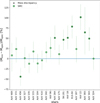 |
Fig. 2 Relative (percentage) difference of the evolutionary and spectroscopic masses (Mevo − Mspec)/Mspec. Mevo was obtained using a Bayesian inference method applied to SMC evolutionary models of Brott et al. (2011). The diagonal black crosses indicate the presence of a mass discrepancy. |
4.2 Stellar masses
Spectroscopic masses, Mspec, presented in Table. A.1, were calculated via  . Since our stars are generally slow rotators, the centrifugal-force corrected gravity, log (gc/cm s−2) = log (g + vrot sin i2/R∗) (Herrero et al. 1992), is very similar to log g. By way of example, log gc log g = 0.02 dex for AzV 372, which has the largest vrot sin i of−our sample (100 km s−1). We also present evolutionary masses, Mevo, and ages, which were obtained using a Bayesian inference method (V. Bronner et al., in prep.) that is similar to BONNSAI (Schneider et al. 2014), applied to Brott et al. (2011) rotating single-star evolutionary models for SMC metallicity.
In Fig. 2, we present the relative difference between Mspec and Mevo for our sample. The error bars representing the uncertainties in Fig. 2 take into account in quadrature the uncertainty of Mevo, which was obtained from the Bayesian inference method, and the uncertainty of Mspec, which in relative terms sits between 25% and 35%. Generally, Mevo is larger than Mspec in our sample. We find that 40% of our sample shows a significant discrepancy between Mspec and Mevo. For these stars, Mevo is larger than Mspec, except for AzV 456, for which we find that Mspec (≈ 83 ± 12 M⊙) is significantly larger than  .
.
Derived wind parameters.
4.3 Wind properties
In Table 4.3, we present the derived wind parameters for our sample. The diverse nature of our sample is shown in the variety of  , covering a range of ≈−8.20 to −5.94 dex. The highest mass-loss rate is attributed to the mid-B hypergiant AzV 393, and the lowest to the late-B supergiant AzV 343.
In Fig. 3, we present our best fits to (red solid line) Hα profiles from XShootU spectra (Sana et al. 2024, DR1). We also include Hα profiles from MIKE observations (Crowther 2024) to illustrate the typical variability of this wind line. We quantify the  variability via test fits to MIKE Hα observations, and obtain
  , which was taken into account when calculating the uncertainties of
  .
.
We obtain satisfactory fits for cases in which the Hα is fully or partially in emission, except for Sk 191, the Hα of which shows a redward radial velocity shift that is not present in other photo-spheric lines. In the cases in which Hα is fully in absorption, we focus on fitting the wings. In any case, when determining  , we take into account the level of saturation of P Cygni profiles. Nevertheless, for cases in which Hα is fully in absorption, we consider the
  presented in Table 4.3 as an upper limit on mass loss.
In Fig. 4, we present a comparison between our derived  and the mass-loss rates predicted by the numerical recipe of Vink & Sander (2021), Björklund et al. (2023), and Krtička et al. (2024), assuming Z = 0.2 Z⊙. We find that for Teff ⪆ 22 kK all recipes perform well and match our derived log M˙ within the uncertainties. For Teff ⪅ 22 kK, which is believed to be the region where the predicted bi-stability jump occurs (Vink et al. 2001), the
  from the recipe of Vink & Sander (2021) predictably become much higher than ours by ≈ 1.5 dex. The recipe of Krtička et al. (2024) continues to perform well on the cool side of the bi-stability jump, whereas the values from the recipe of Björklund et al. (2023) gradually become much smaller than our measurements.
In general,  predictions from numerical recipes agree reasonably well with each other and with empirically derived
  in the O star regime, but deviate greatly from one another and from empirical
  in the B star regime. Recalling the discussion of the evolutionary status of our sample in Section 4.1, we conclude that predictions from numerical recipes are valid for stars on the MS, where massive stars spend most of their lives and where most mass loss takes place. However for post-MS stars, the empirical mass loss rates behave differently than what is predicted by these numerical recipes.
Our sample spans a wide range of v∞ ≈ 160–1800 km s−1. In Fig. 5 we show v∞ versus Teff, with∞our results compared to the empirical recipe of Hawcroft et al. (2024b), results from Bernini-Peron et al. (2024), and velocities calculated from the numerical recipes of Vink & Sander (2021) and (Krtička et al. 2021). We find a difference in the slopes with similar offsets. The main caveat of this comparison is that Hawcroft et al. (2024b) obtained their results by employing the SEI method, fitting only the C iv λ1548 P Cygni for stars no later than B1 and with various luminosity classes. v∞ prediction for Teff values below 21 kK, therefore, should not be considered as reliable.
We fitted our results with a simple linear fit of the form
![Mathematical equation: ${v_\infty }\left[ {{\rm{km}}{{\rm{s}}^{ - 1}}} \right] = a{T_{{\rm{eff }}}}[{\rm{kK}}] - b\left[ {{\rm{km}}{{\rm{s}}^{ - 1}}} \right].$](/articles/aa/full_html/2026/03/aa57856-25/aa57856-25-eq31.png) (4)
(4)
In Table 4, we present the slope, a, and intercept, b, from Equation (4), and compare them to the results of Hawcroft et al. (2024b) and Bernini-Peron et al. (2024). We find that our derived fitting parameters are in excellent agreement with the parameters from (Hawcroft et al. 2024b) when considering only O and B supergiants. We also find excellent agreement with the results of Bernini-Peron et al. (2024).
Our velocities agree with predictions from the recipe of Vink & Sander (2021) below 25 kK, but are lower by ≈30% for temperatures above that threshold. We also find that the recipe from Krtička et al. (2021) systematically overpredicts the velocities by an average of ≈500 km s−1.
Our results in Table 4.3 show that a high β (≈2.5 ± 0.6) is preferred to obtain a satisfactory fit for Hα in the cases in which it is fully or partially in emission. This agrees with the findings of Bernini-Peron et al. (2024), who require β > 2 for most of their SMC sample. Similarly, Crowther et al. (2006) obtained an average β = 2 from a sample of early Galactic B supergiants.
Due to the weakness of the winds of SMC supergiants, and consequently the lack of broad saturated P Cygni profiles in the UV and Hα emission, we were able to constrain fvol,∞ for only nine stars in our sample. We did not find any correlation between fvol,∞ and Teff, Lbol, or  . This is similar to our findings in Paper XIII, and has been the case in recent studies conducting UV and optical spectroscopic analysis of OB stars in multiple environments and utilising various codes with different clumping implementations (Hawcroft et al. 2024a; Bernini-Peron et al. 2024; Verhamme et al. 2024; Brands et al. 2025).
Fitting parameter a (slope) and b (intercept) for Equation (4).
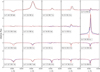 |
Fig. 3 Best fits (solid red lines) to XShootU Hα (+ C ii λ6578) profiles (solid black lines). Magellan/MIKE spectra are also shown (dashed blue lines), where available, to illustrate line variability. |
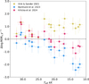 |
Fig. 4
|


4.4 Rotation
In Table A.1, we present vrot sin i of our sample. Our sample spans a range of vrot sin i from 25 km s−1 to 100 km s−1, with a mean vrot sin i of 51 km s−1 and a standard deviation of 19 km s−1. This agrees with the findings of Dufton et al. (2006), who analysed a sample of 24 SMC and Galactic B supergiants and found a linear correlation between vrot and Teff with a value of vrot sin i of ≈60 and 30 km s−1 for Teff = 28 and 12 kK, respectively.
In Table 5, we compare our derived vrot sin i to the vrot sin i and vmac that were obtained from the IACOB-BROAD tool, which employs a combined Fourier transform and goodness-of-fit approach that allows for the extraction of line-broadening parameters (Simón-Díaz & Herrero 2014). We applied IACOB-BROAD to a subsample of our stars with high-resolution MIKE data. The line we used to extract the rotational properties is Si iii λ4552 for the entire subsample, except for the late B super-giants AzV 324 and AzV 343, for which we used Si ii λ6347.
We find that our derived vrot sin i agree with those obtained from IACOB-BROAD within 10 km s−1, except for AzV 104 and AzV 327, where the IACOB-BROAD vrot sin i is 15 and 20 km s−1 higher than ours, respectively. On the other hand, we tend to underestimate vmac on average by ≈20 km s−1. The largest difference in vmac are observed in AzV 327 and AzV 96, for which the values obtained from IACOB-BROAD are higher by 67 and 39 km s−1, respectively.
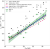 |
Fig. 5 v∞ vs Teff. The green dots represent our results. The green line is the linear fit. The dashed magenta line is the Z-dependent v∞–Teff relation from Hawcroft et al. (2024b). The solid magenta line was obtained from fitting Hawcroft et al. (2024b) results for O and B supergiants only. The solid blue line was obtained from fitting the results of Bernini-Peron et al. (2024). The grey crosses are v∞ calculated from Vink & Sander (2021) recipe. The black triangles represent v∞, calculated from the recipe in Krtička et al. (2021). |
Comparison of our adopted broadening parameters with those obtained via IACOB-BROAD (Simón-Díaz & Herrero 2014) applied to high-resolution MIKE data.
Best-fitting helium (Y, by mass) and CNO (ϵX, by number) abundances.
4.5 Chemical composition
We present the best-fitting chemical abundances for our sample in Table 6. We find moderate helium enhancement for our sample relative to the SMC baseline (Y∼0.25, Russell & Dopita 1990), which is to be expected in a sample comprised of blue super-giants. Fig. 6 shows that all stars in our sample exhibit significant nitrogen enrichment. According to the rotating single-star evolutionary models of Brott et al. (2011) that include rotational mixing, this enrichment can be explained by the high initial rotational velocities (vrot sin i > 300 km s−1), which cause nitrogen synthesised in the interior of the star to be transported to the surface. However, Dufton et al. (2006) found that vrot sin i of SMC B supergiants falls in the range of ≈60–30 km s−1, whereas Mokiem et al. (2006) found that vrot sin i falls in the range of ≈150–180 km s−1 from a diverse sample of SMC O and early B stars.
Spectroscopic studies of the rotational properties of O stars in the SMC, LMC, and the MW show that most early O stars, which are the progenitors of B supergiants, are not fast rotators. Ramachandran et al. (2019) find that ≈75% of SMC O stars have vrot sin i < 200 km s−1. In the Tarantula nebula, Ramírez-Agudelo et al. (2013) find that the distribution of vrot sin i of O stars peaks at ≈80 km s−1. Similarly, (Holgado et al. 2022) find that the distribution of vrot sin i of O stars across all luminosity classes in the MW peaks at ≈80 km s−1.
These observed distributions challenge the assumption that extremely high initial or current rotational velocities are the explanation for the nitrogen enhancement. Only about ≈25% of the massive stars are effectively single, with the overwhelming majority of the fastest rotators being the product of binary interaction (de Mink et al. 2013; Britavskiy et al. 2025; Villaseñor et al. 2025; Bodensteiner et al. 2025; Sana et al. 2025). Therefore, other processes should be considered to explain the nitrogen enhancement, such as binary interaction in the history of the star or the potential existence of a currently undetected companion.
Fig. 7 shows the ratio N/C versus N/O. Following the analytical solution of Maeder et al. (2014), the upper and lower CNO limits (dashed black lines) were calculated using the baseline CNO abundance averages of the SMC from Vink et al. (2023). The majority of our sample falls between the two boundaries and agrees with the expected yield of elements processed by the CNO cycle. The exceptions are AzV 324 and AzV 343, for which we obtained the oxygen abundance by fitting the O i λλλ7772– 7774–7775 multiplet, due to the absence of any other oxygen lines in the optical range. We found that a satisfactory fit to this complex line requires a reduction in the oxygen mass fraction in the model by a factor of four, which explains the high N/O ratios in Fig. 7 for these objects. As is explained in Paper XIII, the O i λλλ7772–7774–7775 multiplet is extremely sensitive to Teff variations at this range; therefore, the oxygen content obtained by fitting those lines is highly uncertain.
Our sample has two stars (AzV 469 and AzV 327) in common with Martins et al. (2024), who employed CMFGEN to obtain the chemical abundances of a sample of SMC and LMC O stars using spectroscopy from ULLYSES and XShootU. We find that our obtained ϵN for these stars agrees within 0.1 dex with their derived nitrogen abundances, whereas carbon and oxygen do not agree so well, though they match within the quoted uncertainties.
We find that the total CNO mass fraction is conserved for most of our sample, except AzV 469, AzV 372, and AzV 215. In the case of these stars, enhanced nitrogen abundances were required to obtain a satisfactory match to the diagnostic lines, and oxygen mass fractions slightly larger than baseline were also required to obtain satisfactory fits for oxygen lines. This explains the implausibly large ratio of cumulative CNO mass fraction to the cumulative solar CNO mass fraction, ΣCNO/ΣCNO⊙. We use these example as a reminder of the large uncertainties associated with the determination of abundances in supergiants from our approach, which are in part due to the sensitivity of the ionisation structure of CNO lines to variations in Teff and log g, but also the fixed micro-turbulent velocity, and the extent of the atomic model adopted in the calculation (number of important levels and superlevels), and the incompleteness of the atomic data.
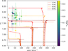 |
Fig. 6 ϵN vs vrot sin i. The colour scheme corresponds to the value of Γe. The solid pink, brown, orange, and red lines represent SMC evolutionary tracks for initial masses of 12 M⊙, 25 M⊙, 40 M⊙, and 60 M⊙, respectively, with initial rotational velocities of 110, 250, 350 km s−1 (Brott et al. 2011). We multiplied by a factor of π/4 to take into account the inclination of the rotation axis (Hunter et al. 2008). The dashed black line represents the baseline ϵN in the SMC (Vink et al. 2023). The dots along the evolutionary tracks represent time steps of 0.1 Myr. |
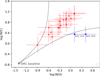 |
Fig. 7 log N/C vs log N/O. The red triangles show the distribution of our sample. The stars for which the oxygen abundance was obtained from fitting the O i λλλ7772–7774–7775 multiplet are shown in blue squares. The dashed black lines represent the upper and lower boundaries adopted from Maeder et al. (2014). |
Slopes, x, and vertical offsets, log D0, of Equation (5) of this study and from Paper XIII.
5 Discussion
5.1 Metallicity effect
Fig. 8 shows the modified wind momentum, which was introduced by Kudritzki et al. (1999) as  , as a function of Lbol. We fitted our derived values using the relation
 (5)
(5)
In Fig. 8, solid lines are fits to the stars (circles) that show both P Cygni profiles in the UV and Hα in emission, making their determined wind parameters the most reliable. We can see that including stars with Hα in absorption (triangles) in the linear fit slightly changes the slope of the fit for the LMC sample from Paper XII (dash-dotted green line). Doing the same for our SMC sample decreases the vertical offset of the fit (dash-dotted yellow line), albeit very slightly.
In Table 7, we present the best fitting parameters of Equation (5) (slopes, x, and offsets, log D0). Comparing the Dmom of the current SMC sample to the LMC sample analysed in Paper XIII, we find that the slope of the SMC is slightly steeper than the LMC, albeit quite similar. We also find a large difference in the intercepts between the two samples, which can be attributed to the Z dependence of wind properties.
In Figure 9, we show v∞ as a function of Teff of the present study compared to the results from Paper XIII. Figure 10 shows  vs log Lbol from this study compared to Paper XIII. 3 does not show signs of Z dependence, whereas
  shows a clear offset between the two samples, indicating a strong Z dependence. Therefore, we can assume that the Z dependence of Dmom is dominated by the Z dependence of
  .
.
In parallel with our study, Verhamme et al. (2025) have recently undertaken an analysis of ULLYSES/XShootU SMC B supergiants. To investigate the effect of metallicity, they compare their analysis to an earlier study of LMC B supergiants (Verhamme et al. 2024). Despite our overlapping samples, they arrived at different conclusions, which is discussed further in Appendix B.
Following Krtička & Kubát (2018) and Backs et al. (2024), we obtained an equation for the Z-dependent log Dmom of the form
 (6)
(6)
where from Equation (5)  , and a, b, c, and d are fitting parameters. fitting are presented in Table 8, assuming that ZLMC = 0.5Z⊙ and ZSMC = 0.2Z⊙. We also include values from Backs et al. (2024) in Table 8.
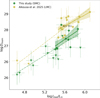 |
Fig. 8 Dmom vs logLbol. The green symbols represent the SMC sample. The yellow symbols represent the LMC sample from Paper XIII. Circles indicate stars with reliable UV and optical wind diagnostics. Triangles indicate upper limits. Solid lines are fits to the circles. Dash-dotted lines are fits for the entire sample. |

Fitting parameter of Equation (6).
5.2 Bi-stability jump
In Fig. 11, we present our derived  in terms of Teff. This confirms that AzV 393 possesses much higher
  , not just compared to objects with similar Teff, but even compared to the hotter OB supergiants in our sample. We do not find any sign of a large increase in
  around 25–21 kK, which could be attributed to the bi-stability jump. Using a simple linear regression, we find that
  is constant with Teff (solid blue line). Excluding the hyper-giant AzV 393 from the fit (dashed blue line), we find that log M˙ decreases with Teff.
To investigate the effect of luminosity, we calculated the transformed mass-loss rate, which is defined as
 (7)
(7)
In Fig. 12, we compare  to Teff. We find that when including or excluding AzV 393 in the linear fit,
  increases with temperature. This is in contrast to the results of Bernini-Peron et al. (2024), which hint at a constant behaviour of the mass-loss rate with temperature. The reason for this trend could be our comparably low values of fvol,∞ < 0.2 (i.e. a high degree of clumping in the winds), which lowers the mass-loss rates required to obtain a satisfactory fit to Hα and to the UV P Cygni profiles.
In Fig. 13, we present the ratio v∞ to the escape velocity vesc as a function of Teff, which was calculated using Mevo. From our results, we derive a relation of
 (8)
(8)
Where  , and Γe is the Eddington parameter, which was calculated using Mevo.
We do not notice any drastic decrease in v∞/vesc below Teff = 25-21 kK, indicative of the theorised bi-stability jump. We find that v∞/vesc decreases monotonically with Teff. These results show a lack of evidence for the existence of the bi-stability jump, which is similar to the findings of Paper XIII, as well as the findings of de Burgos et al. (2024a) in the MW, Bernini-Peron et al. (2024) in the SMC, and Verhamme et al. (2024) in the LMC. In Appendix C, we include some additional discussion on the bi-stability jump.
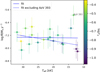 |
Fig. 11
|


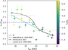 |
Fig. 13 Ratio (v∞/vesc) as a function of temperature. The solid green line represents the linear fit to our sample. The dashed black line is the relation presented in Krtička et al. (2021). The dotted red lines represent the ratios from Lamers et al. (1995). The colour gradient correlates with the value of Γe. |
5.3 Implications for the population of blue supergiants
Recalling the HRD in Fig. 1, the shaded region is defined by the observed HD limit (Humphreys & Davidson 1979, 1994) in the SMC, which has a value of log Lbol/L⊙≈ 5.5 (Davies et al. 2018). The diagonal blue edge of this region is inferred from the distribution of known luminous blue variables (LBVs) and LBV candidates on the HRD (Smith et al. 2004).
The HD limit suggests that the most massive stars with luminosities higher than log Lbol/L⊙ ≈ 5.5 remain as blue super-giants, and end their lives as blue hypergiants and classical Wolf-Rayet (WR) stars, rather than evolving into luminous red supergiants. This means that, at least in theory, they should have sufficiently high mass-loss rates to shed their hydrogen-rich atmospheres and proceed to a classical WR phase. The existence of a considerable non-binary population of WRs in the SMC (e.g. Hainich et al. 2015; Schootemeijer et al. 2024) with high luminosity, for which Shenar et al. (2020) finds a non-binary fraction of ≈60-70%, in addition to a lower limit on WR luminosity of log Lbol/L⊙ = 5.6, which is comparable to the uppermost part of our sample and could, in principle, be seen as an argument for a self-stripping evolutionary scenario via extreme LBV eruptions.
However, aligning this evolutionary scenario with the mass-loss rates obtained in studies of blue supergiants in the SMC (This study, Bernini-Peron et al. 2024; Trundle & Lennon 2005; Trundle et al. 2004) poses a challenge for explaining the formation of WR stars from radiation-driven mass loss alone in the single-star regime. By way of example, AzV 242 has an evolutionary mass of  , a luminosity of log Lbol/L⊙ = 5.71 ± 0.1, and a mass-loss rate of
  . AzV 242 closely corresponds to the minimum initial mass of WR stars in the SMC (Shenar et al. 2020), yet the mass-loss rate of this supergiant is far too low to result in the stripping of the outer hydrogen-rich layers within its remaining ∼0.5 Myr lifetime.
The low current mass-loss rates, together with the observed properties of WR populations and the lack of luminous red supergiants in the SMC, leads to the following conclusion: to form a WR star via single-star evolution, luminous blue super-giants would need to lose copious amounts of mass during an LBV giant eruption (Smith 2017; Jiang et al. 2018). This is supported by recent work from Pauli et al. (2026), who were able to replicate the observed properties of the WR and RSG populations – including the low-luminosity single WRs – in the SMC by incorporating LBV-like Eddington-limit induced mass loss in evolutionary models. It is also probable that binarity, mass transfer via Roche lobe overflow, and common envelope evolution play a significant role in shaping the WR population (Schootemeijer & Langer 2018).
6 Summary and conclusions
We have completed a spectroscopic analysis of 20 late-O and B SMC supergiants, which employed CMFGEN (Hillier & Miller 1998), using the UV (ULLYSES) and optical (XShootU) spectral ranges. We obtained stellar and wind parameters of the stars in our sample. By comparing our results to those of Alkousa et al. (2025) for the LMC, we find a clear Z dependence in wind momentum, which is shown in Fig. 8. We derived the wind momentum-luminosity relation presented in Equation (6). We also found a clear Z dependence in mass-loss rates, but did not find similar Z dependence in the terminal wind velocities.
We compared our derived mass-loss rates to predictions from various numerical recipes Vink & Sander (2021); Björklund et al. (2023); Krtička et al. (2024). We found that the values of the numerical recipes differ from our mass-loss rates, with the recipe from Krtička et al. (2024) producing the values most closely aligned with ours, yet still showing a different trend with temperature.
We also compared our results to literature values of the same stars (Trundle et al. 2004; Trundle & Lennon 2005; Backs et al. 2024; Bernini-Peron et al. 2024; Bestenlehner et al. 2025). On the one hand, we find that the effective temperature, surface gravity, and luminosity generally agree with previous studies with modest variance. However, our derived mass-loss rates do not match previous estimates, with our values being generally lower than those previously obtained by previous studies.
We do not find any sign of the theorised bi-stability jump. This is similar to the findings of de Burgos et al. (2024a), Bernini-Peron et al. (2024), Verhamme et al. (2024), and Alkousa et al. (2025). This means that within the current framework of radiative transfer codes used for modelling OB stars, the dramatic increase in mass loss at Teff = 25–21 kK that is associated with the theorised bi-stability jump is not empirically supported.
We also explored the evolutionary history of the stars within our sample. We employed an updated Bayesian inference method (V. Bronner et al., in prep.) similar to BONNSAI (Schneider et al. 2014) to obtain the evolutionary masses and ages using the rotating single-star evolutionary tracks of Brott et al. (2011). Evolutionary masses typically exceed spectroscopic masses, with 40% of our sample showing a mass discrepancy.
Finally, we emphasise that mass-loss rates of supergiants exceeding the HD limit of log Lbol/L⊙ = 5.5 (Davies et al. 2018) are far too low to be able to strip the supergiants of their hydrogen-rich outer layers. Consequently, the high fraction of single WR stars observed in the SMC (Shenar et al. 2020) cannot be explained by the classical single star evolutionary regime, unless the supergiant is capable of losing an enormous amount of mass within its very short remaining lifespan. This possibly means that an intermediate LBV phase that is accompanied by extreme episodic eruptions and mass loss is required for the star to proceed into a WR phase.
In the next installment of this series of papers, we plan to analyse a similar sample of Galactic blue supergiants using the same methods as are presented in Paper XIII. This will allow us to derive a mass-loss rate recipe for supergiants, which avoids differences introduced by utilising various analysis techniques and codes.
Data availability
The supplementary online material can be found on Zenodo1. Appendix G includes comments on diagnostic-line fits for all the targets in our sample. Additionally, SED fits, diagnostic-line fits, and overall UV and optical spectral fits can be found in Appendix H, I, and Appendix J, respectively.
Acknowledgements
TA would like to thank the Science and Technology Facilities Council (STFC) for financial support through the STFC scholarship ST/X508743/1. RK acknowledges financial support via the Heisen-berg Research Grant funded by the Deutsche Forschungsgemeinschaft (DFG, German Research Foundation) under grant no. KU 2849/9, project no. 445783058. F.N., acknowledges support by PID2022-137779OB-C41 funded by MCIN/AEI/10.13039/501100011033 by “ERDF A way of making Europe”. AACS and MBP are supported by the German Deutsche Forschungsgemein-schaft, DFG in the form of an Emmy Noether Research Group – Project-ID 445674056 (SA4064/1-1, PI Sander). This project was co-funded by the Euro-pean Union (Project 101183150 – OCEANS).This study was made possible through the Director’s discretionary ULLYSES survey, which was implemented by a Space Telescope Science Institute (STScI) team led by Julia Roman-Duval. Based on observations made with ESO telescopes at the Paranal observatory under programme ID 106.211Z.001 and observations obtained with the NASA/ESA Hubble Space Telescope, retrieved from the Mikulski Archive for Space Telescopes (MAST) at the STScI. STScI is operated by the Association of Universities for Research in Astronomy, Inc. under NASA contract NAS 5-26555. We also thank John Hillier for developing CMFGEN, Nidia Morrell for obtaining and reducing MIKE data in addition to her feedback on this paper, and Vincent Bronner for facilitating the use of his Bayesian inference technique. This research has used the SIMBAD database, operated at CDS, Strasbourg, France. We would like to thank the referee for their critical and insightful comments.
References
- Abbott, D. C. 1982, ApJ, 259, 282 [Google Scholar]
- Alkousa, T., Crowther, P. A., Bestenlehner, J. M., et al. 2025, A&A, 699, A314 [NASA ADS] [CrossRef] [EDP Sciences] [Google Scholar]
- Anderson, L. S. 1985, ApJ, 298, 848 [NASA ADS] [CrossRef] [Google Scholar]
- Anderson, L. S. 1989, ApJ, 339, 558 [Google Scholar]
- Ardeberg, A. 1980, A&AS, 42, 1 [Google Scholar]
- Ardeberg, A., & Maurice, E. 1977, A&AS, 30, 261 [Google Scholar]
- Azzopardi, M., Vigneau, J., & Macquet, M. 1975, A&AS, 22, 285 [Google Scholar]
- Backs, F., Brands, S. A., de Koter, A., et al. 2024, A&A, 692, A88 [NASA ADS] [CrossRef] [EDP Sciences] [Google Scholar]
- Beckman, J. E., & Crivellari, L. 1985, Science, 230, 835 [Google Scholar]
- Bernini-Peron, M., Sander, A. A. C., Ramachandran, V., et al. 2024, A&A, 692, A89 [NASA ADS] [CrossRef] [EDP Sciences] [Google Scholar]
- Bestenlehner, J. M., Enßlin, T., Bergemann, M., et al. 2024, MNRAS, 528, 6735 [CrossRef] [Google Scholar]
- Bestenlehner, J. M., Crowther, P. A., Hawcroft, C., et al. 2025, A&A, 695, A198 [NASA ADS] [CrossRef] [EDP Sciences] [Google Scholar]
- Björklund, R., Sundqvist, J. O., Singh, S. M., Puls, J., & Najarro, F. 2023, A&A, 676, A109 [NASA ADS] [CrossRef] [EDP Sciences] [Google Scholar]
- Bodensteiner, J., Shenar, T., Sana, H., et al. 2025, A&A, 698, A38 [NASA ADS] [CrossRef] [EDP Sciences] [Google Scholar]
- Brands, S. A., Backs, F., de Koter, A., et al. 2025, A&A, 697, A54 [NASA ADS] [CrossRef] [EDP Sciences] [Google Scholar]
- Bresolin, F., Kudritzki, R.-P., & Urbaneja, M. A. 2022, ApJ, 940, 32 [NASA ADS] [CrossRef] [Google Scholar]
- Britavskiy, N., Mahy, L., Lennon, D. J., et al. 2025, A&A, 698, A40 [NASA ADS] [CrossRef] [EDP Sciences] [Google Scholar]
- Brott, I., de Mink, S. E., Cantiello, M., et al. 2011, A&A, 530, A115 [NASA ADS] [CrossRef] [EDP Sciences] [Google Scholar]
- Castor, J. I., Abbott, D. C., & Klein, R. I. 1975, ApJ, 195, 157 [Google Scholar]
- Castor, J. I., & Lamers, H. J. G. L. M. 1979, ApJS, 39, 481 [NASA ADS] [CrossRef] [Google Scholar]
- Cioni, M. R., Clementini, G., Girardi, L., et al. 2011, The Messenger, 144, 25 [NASA ADS] [Google Scholar]
- Conti, P. S., & Ebbets, D. 1977, ApJ, 213, 438 [CrossRef] [Google Scholar]
- Crowther, P. A. 2024, in IAU Symposium, 361, IAU Symposium, eds. J. Mackey, J. S. Vink, & N. St-Louis, 15 [Google Scholar]
- Crowther, P. A., Lennon, D. J., & Walborn, N. R. 2006, A&A, 446, 279 [NASA ADS] [CrossRef] [EDP Sciences] [Google Scholar]
- Cutri, R. M., Skrutskie, M. F., van Dyk, S., et al. 2003, VizieR On-line Data Catalog: II/246. Originally published in: University of Massachusetts and Infrared Processing and Analysis Center, (IPAC/California Institute of Technology) [Google Scholar]
- Cutri, R. M., Skrutskie, M. F., van Dyk, S., et al. 2012, VizieR On-line Data Catalog: II/281. Originally published in: 2012yCat.2281….0C [Google Scholar]
- Danforth, C. W., Howk, J. C., Fullerton, A. W., Blair, W. P., & Sembach, K. R. 2002, ApJS, 139, 81 [Google Scholar]
- Davies, B., Crowther, P. A., & Beasor, E. R. 2018, MNRAS, 478, 3138 [NASA ADS] [CrossRef] [Google Scholar]
- de Burgos, A., Keszthelyi, Z., Simón-Díaz, S., & Urbaneja, M. A. 2024a, A&A, 687, L16 [NASA ADS] [CrossRef] [EDP Sciences] [Google Scholar]
- de Burgos, A., Simón-Díaz, S., Urbaneja, M. A., & Puls, J. 2024b, A&A, 687, A228 [NASA ADS] [CrossRef] [EDP Sciences] [Google Scholar]
- de Mink, S. E., Langer, N., Izzard, R. G., Sana, H., & de Koter, A. 2013, ApJ, 764, 166 [Google Scholar]
- Dufton, P. L., Ryans, R. S. I., Simón-Díaz, S., Trundle, C., & Lennon, D. J. 2006, A&A, 451, 603 [NASA ADS] [CrossRef] [EDP Sciences] [Google Scholar]
- Eddington, A. S. 1926, The Internal Constitution of the Stars [Google Scholar]
- Evans, C. J., Lennon, D. J., Walborn, N. R., Trundle, C., & Rix, S. A. 2004, PASP, 116, 909 [NASA ADS] [CrossRef] [Google Scholar]
- Fitzpatrick, E. L., & Massa, D. 1990, ApJS, 72, 163 [NASA ADS] [CrossRef] [Google Scholar]
- Fouesneau, M. 2025, pyphot: A tool for computing photometry from spectra, https://github.com/mfouesneau/pyphot [Google Scholar]
- Geen, S., Agrawal, P., Crowther, P. A., et al. 2023, PASP, 135, 021001 [NASA ADS] [CrossRef] [Google Scholar]
- Gordon, K. D., Clayton, G. C., Misselt, K. A., Landolt, A. U., & Wolff, M. J. 2003, ApJ, 594, 279 [NASA ADS] [CrossRef] [Google Scholar]
- Graczyk, D., Pietrzyński, G., Thompson, I. B., et al. 2020, ApJ, 904, 13 [Google Scholar]
- Green, J. C., Froning, C. S., Osterman, S., et al. 2012, ApJ, 744, 60 [NASA ADS] [CrossRef] [Google Scholar]
- Hainich, R., Pasemann, D., Todt, H., et al. 2015, A&A, 581, A21 [NASA ADS] [CrossRef] [EDP Sciences] [Google Scholar]
- Hardorp, J., & Scholz, M. 1970, ApJS, 19, 193 [Google Scholar]
- Hawcroft, C., Mahy, L., Sana, H., et al. 2024a, A&A, 690, A126 [NASA ADS] [CrossRef] [EDP Sciences] [Google Scholar]
- Hawcroft, C., Sana, H., Mahy, L., et al. 2024b, A&A, 688, A105 [NASA ADS] [CrossRef] [EDP Sciences] [Google Scholar]
- Herrero, A., Kudritzki, R. P., Vilchez, J. M., et al. 1992, A&A, 261, 209 [NASA ADS] [Google Scholar]
- Hillier, D. J. 1990, A&A, 231, 116 [NASA ADS] [Google Scholar]
- Hillier, D. J. 1996, in Liege International Astrophysical Colloquia, 33, Liege International Astrophysical Colloquia, eds. J. M. Vreux, A. Detal, D. Fraipont-Caro, E. Gosset, & G. Rauw, 509 [Google Scholar]
- Hillier, D. J. 1997, in IAU Symposium, 189, IAU Symposium, eds. T. R. Bedding, A. J. Booth, & J. Davis, 209 [Google Scholar]
- Hillier, D. J., & Miller, D. L. 1998, ApJ, 496, 407 [NASA ADS] [CrossRef] [Google Scholar]
- Hillier, D. J., & Miller, D. L. 1999, ApJ, 519, 354 [Google Scholar]
- Holgado, G., Simón-Díaz, S., Herrero, A., & Barbá, R. H. 2022, A&A, 665, A150 [NASA ADS] [CrossRef] [EDP Sciences] [Google Scholar]
- Humphreys, R. M., & Davidson, K. 1979, ApJ, 232, 409 [Google Scholar]
- Humphreys, R. M., & Davidson, K. 1994, PASP, 106, 1025 [NASA ADS] [CrossRef] [Google Scholar]
- Hunter, I., Brott, I., Lennon, D. J., et al. 2008, ApJ, 676, L29 [NASA ADS] [CrossRef] [Google Scholar]
- Jiang, Y.-F., Cantiello, M., Bildsten, L., et al. 2018, Nature, 561, 498 [NASA ADS] [CrossRef] [Google Scholar]
- Krtička, J., & Kubát, J. 2018, A&A, 612, A20 [NASA ADS] [CrossRef] [EDP Sciences] [Google Scholar]
- Krtička, J., Kubát, J., & Krtičková, I. 2021, A&A, 647, A28 [NASA ADS] [CrossRef] [EDP Sciences] [Google Scholar]
- Krtička, J., Kubát, J., & Krtičková, I. 2024, A&A, 681, A29 [NASA ADS] [CrossRef] [EDP Sciences] [Google Scholar]
- Kudritzki, R. P., Pauldrach, A., & Puls, J. 1987, A&A, 173, 293 [NASA ADS] [Google Scholar]
- Kudritzki, R. P., Puls, J., Lennon, D. J., et al. 1999, A&A, 350, 970 [Google Scholar]
- Kudritzki, R. P., Bresolin, F., & Przybilla, N. 2003, ApJ, 582, L83 [Google Scholar]
- Kudritzki, R.-P., Urbaneja, M. A., Bresolin, F., et al. 2008, ApJ, 681, 269 [NASA ADS] [CrossRef] [Google Scholar]
- Kudritzki, R.-P., Urbaneja, M. A., Bresolin, F., et al. 2024, ApJ, 977, 217 [Google Scholar]
- Lamers, H. J. G. L. M., Snow, T. P., & Lindholm, D. M. 1995, ApJ, 455, 269 [Google Scholar]
- Langer, N. 2012, Annu. Rev. Astron. Astrophys., 50, 107 [Google Scholar]
- Lanz, T., & Hubeny, I. 2007, ApJS, 169, 83 [CrossRef] [Google Scholar]
- Leitherer, C., Robert, C., & Drissen, L. 1992, ApJ, 401, 596 [Google Scholar]
- Lennon, D. J., Dufton, P. L., & Fitzsimmons, A. 1992, A&AS, 94, 569 [Google Scholar]
- Lucy, L. B., & Solomon, P. M. 1970, ApJ, 159, 879 [Google Scholar]
- Maeder, A., Przybilla, N., Nieva, M.-F., et al. 2014, A&A, 565, A39 [NASA ADS] [CrossRef] [EDP Sciences] [Google Scholar]
- Marcolino, W. L. F., Bouret, J. C., Rocha-Pinto, H. J., Bernini-Peron, M., & Vink, J. S. 2022, MNRAS, 511, 5104 [NASA ADS] [CrossRef] [Google Scholar]
- Martins, F. 2011, Bull. Soc. Roy. Sci. Liege, 80, 29 [Google Scholar]
- Martins, F., Bouret, J. C., Hillier, D. J., et al. 2024, A&A, 689, A31 [NASA ADS] [CrossRef] [EDP Sciences] [Google Scholar]
- Massa, D. L., Prinja, R. K., & Fullerton, A. W. 2008, in Clumping in Hot-Star Winds, eds. W.-R. Hamann, A. Feldmeier, & L. M. Oskinova, 147 [Google Scholar]
- Massey, P. 2002, ApJS, 141, 81 [NASA ADS] [CrossRef] [Google Scholar]
- McErlean, N. D., Lennon, D. J., & Dufton, P. L. 1998, A&A, 329, 613 [NASA ADS] [Google Scholar]
- McErlean, N. D., Lennon, D. J., & Dufton, P. L. 1999, A&A, 349, 553 [NASA ADS] [Google Scholar]
- Mokiem, M. R., de Koter, A., Evans, C. J., et al. 2006, A&A, 456, 1131 [NASA ADS] [CrossRef] [EDP Sciences] [Google Scholar]
- Mokiem, M. R., de Koter, A., Vink, J. S., et al. 2007, A&A, 473, 603 [NASA ADS] [CrossRef] [EDP Sciences] [Google Scholar]
- Moos, H. W., Cash, W. C., Cowie, L. L., et al. 2000, ApJ, 538, L1 [NASA ADS] [CrossRef] [Google Scholar]
- Nieva, M. F. 2013, A&A, 550, A26 [CrossRef] [EDP Sciences] [Google Scholar]
- Pauli, D., Oskinova, L. M., Hamann, W. R., et al. 2025, A&A, 697, A114 [NASA ADS] [CrossRef] [EDP Sciences] [Google Scholar]
- Pauli, D., Langer, N., Schootemeijer, A., et al. 2026, A&A, 707, A11 [NASA ADS] [CrossRef] [EDP Sciences] [Google Scholar]
- Prinja, R. K., & Crowther, P. A. 1998, MNRAS, 300, 828 [NASA ADS] [CrossRef] [Google Scholar]
- Prinja, R. K., Barlow, M. J., & Howarth, I. D. 1990, ApJ, 361, 607 [NASA ADS] [CrossRef] [Google Scholar]
- Puls, J., Kudritzki, R. P., Herrero, A., et al. 1996, A&A, 305, 171 [Google Scholar]
- Puls, J., Urbaneja, M. A., Venero, R., et al. 2005, A&A, 435, 669 [NASA ADS] [CrossRef] [EDP Sciences] [Google Scholar]
- Puls, J., Vink, J. S., & Najarro, F. 2008, A&A Rev., 16, 209 [Google Scholar]
- Ramachandran, V., Hamann, W. R., Oskinova, L. M., et al. 2019, A&A, 625, A104 [NASA ADS] [CrossRef] [EDP Sciences] [Google Scholar]
- Ramírez-Agudelo, O. H., Simón-Díaz, S., Sana, H., et al. 2013, A&A, 560, A29 [NASA ADS] [CrossRef] [EDP Sciences] [Google Scholar]
- Rivero González, J. G., Puls, J., & Najarro, F. 2011, A&A, 536, A58 [NASA ADS] [CrossRef] [EDP Sciences] [Google Scholar]
- Roman-Duval, J., Fischer, W. J., Fullerton, A. W., et al. 2025, ApJ, 985, 109 [Google Scholar]
- Russell, S. C., & Dopita, M. A. 1990, ApJS, 74, 93 [NASA ADS] [CrossRef] [Google Scholar]
- Sana, H., Tramper, F., Abdul-Masih, M., et al. 2024, A&A, 688, A104 [NASA ADS] [CrossRef] [EDP Sciences] [Google Scholar]
- Sana, H., Shenar, T., Bodensteiner, J., et al. 2025, Nat. Astron., 9, 1337 [Google Scholar]
- Sander, A. A. C., Bouret, J. C., Bernini-Peron, M., et al. 2024, A&A, 689, A30 [NASA ADS] [CrossRef] [EDP Sciences] [Google Scholar]
- Schmutz, W., Hamann, W. R., & Wessolowski, U. 1989, A&A, 210, 236 [Google Scholar]
- Schneider, F. R. N., Langer, N., de Koter, A., et al. 2014, A&A, 570, A66 [NASA ADS] [CrossRef] [EDP Sciences] [Google Scholar]
- Schootemeijer, A., & Langer, N. 2018, A&A, 611, A75 [NASA ADS] [CrossRef] [EDP Sciences] [Google Scholar]
- Schootemeijer, A., Shenar, T., Langer, N., et al. 2024, A&A, 689, A157 [NASA ADS] [CrossRef] [EDP Sciences] [Google Scholar]
- Scowcroft, V., Freedman, W. L., Madore, B. F., et al. 2016, ApJ, 816, 49 [NASA ADS] [CrossRef] [Google Scholar]
- Searle, S. C., Prinja, R. K., Massa, D., & Ryans, R. 2008, A&A, 481, 777 [NASA ADS] [CrossRef] [EDP Sciences] [Google Scholar]
- Shenar, T., Gilkis, A., Vink, J. S., Sana, H., & Sander, A. A. C. 2020, A&A, 634, A79 [NASA ADS] [CrossRef] [EDP Sciences] [Google Scholar]
- Shenar, T., Bodensteiner, J., Sana, H., et al. 2024, A&A, 690, A289 [NASA ADS] [CrossRef] [EDP Sciences] [Google Scholar]
- Simón-Díaz, S., & Herrero, A. 2014, A&A, 562, A135 [NASA ADS] [CrossRef] [EDP Sciences] [Google Scholar]
- Simón-Díaz, S., Herrero, A., Uytterhoeven, K., et al. 2010, ApJ, 720, L174 [CrossRef] [Google Scholar]
- Skrutskie, M. F., Cutri, R. M., Stiening, R., et al. 2006, AJ, 131, 1163 [NASA ADS] [CrossRef] [Google Scholar]
- Slettebak, A. 1956, ApJ, 124, 173 [NASA ADS] [CrossRef] [Google Scholar]
- Smartt, S. J. 2009, ARA&A, 47, 63 [Google Scholar]
- Smith, N. 2014, ARA&A, 52, 487 [Google Scholar]
- Smith, N. 2017, Philos. Trans. Roy. Soc. Lond. Ser. A, 375, 20160268 [Google Scholar]
- Smith, N., Vink, J. S., & de Koter, A. 2004, ApJ, 615, 475 [NASA ADS] [CrossRef] [Google Scholar]
- Sundqvist, J. O., Debnath, D., Backs, F., et al. 2025, A&A, 703, A284 [NASA ADS] [CrossRef] [EDP Sciences] [Google Scholar]
- Trundle, C., & Lennon, D. J. 2005, A&A, 434, 677 [NASA ADS] [CrossRef] [EDP Sciences] [Google Scholar]
- Trundle, C., Lennon, D. J., Puls, J., & Dufton, P. L. 2004, A&A, 417, 217 [NASA ADS] [CrossRef] [EDP Sciences] [Google Scholar]
- Trundle, C., Dufton, P. L., Hunter, I., et al. 2007, 471, 625 [Google Scholar]
- Urbaneja, M. A., Herrero, A., Bresolin, F., et al. 2005a, ApJ, 622, 862 [Google Scholar]
- Urbaneja, M. A., Herrero, A., Kudritzki, R. P., et al. 2005b, ApJ, 635, 311 [NASA ADS] [CrossRef] [Google Scholar]
- Urbaneja, M. A., Kudritzki, R. P., Gieren, W., et al. 2017, AJ, 154, 102 [NASA ADS] [CrossRef] [Google Scholar]
- Verhamme, O., Sundqvist, J., de Koter, A., et al. 2024, A&A, 692, A91 [NASA ADS] [CrossRef] [EDP Sciences] [Google Scholar]
- Verhamme, O., Sundqvist, J., & XShootU Collaboration. 2025, A&A [Google Scholar]
- Vernet, J., Dekker, H., D’Odorico, S., et al. 2011, A&A, 536, A105 [NASA ADS] [CrossRef] [EDP Sciences] [Google Scholar]
- Villaseñor, J. I., Sana, H., Mahy, L., et al. 2025, A&A, 698, A41 [NASA ADS] [CrossRef] [EDP Sciences] [Google Scholar]
- Vink, J. S., & Sander, A. A. C. 2021, MNRAS, 504, 2051 [NASA ADS] [CrossRef] [Google Scholar]
- Vink, J. S., de Koter, A., & Lamers, H. J. G. L. M. 1999, A&A, 350, 181 [Google Scholar]
- Vink, J. S., de Koter, A., & Lamers, H. J. G. L. M. 2001, A&A, 369, 574 [NASA ADS] [CrossRef] [EDP Sciences] [Google Scholar]
- Vink, J. S., Mehner, A., Crowther, P. A., et al. 2023, A&A, 675, A154 [NASA ADS] [CrossRef] [EDP Sciences] [Google Scholar]
- Walborn, N. R., Lennon, D. J., Heap, S. R., et al. 2000, PASP, 112, 1243 [Google Scholar]
- Walborn, N. R., Fullerton, A. W., Crowther, P. A., et al. 2002, ApJS, 141, 443 [NASA ADS] [CrossRef] [Google Scholar]
- Woodgate, B. E., Kimble, R. A., Bowers, C. W., et al. 1998, PASP, 110, 1183 [NASA ADS] [CrossRef] [Google Scholar]
Appendix A Main results table
Derived stellar parameters based on the best fitting CMFGEN model.
In Table A.1, Minit, Mevo, and ages of the stars are derived using an updated Bayesian inference method (Bronner et al. in prep) that is similar to BONNSAI (Schneider et al. 2014) applied to Brott et al. (2011) SMC evolutionary tracks. The average uncertainty in Teff is ∆Teff = 1 kK. In the uncertainties of centrifugal force-corrected surface gravity log gc, we take into account the fitting uncertainty of log g and the uncertainty of the projected rotational velocity vrot sin i and the radius R∗. We find a mean uncertainty of ∆ log gc = 0.2 dex. The uncertainty in radial velocity vrad measurements is dominated by the velocity resolution of the UBV part of the spectrum which is ∆v ≈ 45 km s−1. The total extinction AV (∆AV ≈ 0.02 mag), absolute V-band magnitude MV, and bolometric correction BCV are produced from the SED fits.  is subject to uncertainties of
  which takes into account the uncertainties of Mspec and log Lbol
Appendix B Additional discussion on Z dependence
In parallel with the present study, Verhamme et al. (2025) have analysed a sample of ULLYSES/XShootU SMC B supergiants using KIWI-GA. They find broadly comparable mass-loss rates and wind momenta with respect to LMC B supergiants (Verhamme et al. 2024), in contrast with our results, despite having 13 stars in common with our sample.
This surprising result could be attributed to a number of issues. Firstly, the determination of robust wind parameters of late B supergiants in the SMC is particularly challenging due to the lack of wind diagnostics, and the current version of FAST-WIND is known to have convergence difficulties below 14 kK (de Burgos et al. 2024b). These issues could have skewed KIWI-GA solutions to higher Dmom. This is confirmed when examining the Hα fits of Verhamme et al. (2025), where the preferred solution overpredicts Hα emission. In addition, their derived Teff often deviates quite significantly from the usual spectral type – temperature scale of B supergiants (see e.g. Lanz & Hubeny 2007; Trundle et al. 2007; Nieva 2013). By way of example, Ver-hamme et al. (2025) obtained a lower Teff for AzV 410 (B0.7 Iab) than NGC330 ELS 4 (B2.5 Ib).
Appendix C Additional discussion of wind parameters and the bi-stability jump
In Fig. C.1, we show the wind efficiency parameter  versus Teff. We find that η smoothly decreases with Teff. One extreme outlier is the hypergiant AzV 393, which has a very high
  . Another outlier is AzV 456, which has a very low η. This is due to its v∞, which is lower by ≈300 km s−1 compared to AzV 327, which has a very similar Teff.
Appendix D CNO diagnostics
Table D.1 shows the diagnostic lines used to constrain the surface abundances of carbon, nitrogen, and oxygen. It also shows the spectral type range in which each metal line is used.
Appendix E vblack and vedge
In Table E.1 we present the measured vedge and 3black from each line for all our sample.
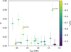 |
Fig. C.1 Wind efficiency |

Line diagnostics for determination of CNO elemental abundances.
vedge and vblack for the stars in our sample.
Appendix F Comparison to literature
Table F.1 contains our derived values for Teff, log g, Lbol, log  , β, and fvol,∞, along with literature values from Trundle et al. (2004), Trundle & Lennon (2005), Bernini-Peron et al. (2024), Backs et al. (2024), and Bestenlehner et al. (2025). The volume-filling factor for studies that used the optically thick clumping implementation in FASTWIND is calculated from the equation introduced in Sander et al. (2024) following:
 (F.1)
(F.1)
where fcl = ⟨ρ2⟩/⟨ρ⟩2 describes the contrast between the density in the clump and the mean density, and fic describes the contrast between the clump density and the density of the inter-clump medium.
In addition to literature values, Table F.1 in includes  values obtained from LIME (Sundqvist et al. 2025). LIME is a user-friendly and fast online tool that allows for the estimation of the mass-loss rates of stars using an iterative semi-analytic approach using an extension of the Castor et al. (1975) concept. By including a detailed list of atomic lines, but avoiding a numerical solution for the equation of motion and the stellar atmosphere, the tool can estimate M˙ on the fly, in contrast to the recipes discussed in Section 4.3, which result from approximating sets of detailed numerical models. The input parameters we used for LIME are our derived Teff, Lbol, Mspec, mass fractions of H, He, C, N, O, and the mean mass fractions for elements heavier than oxygen presented in Vink et al. (2023). In Fig. F.1 we compare our obtained values Teff, log g, Lbol,
  , and
, and  to the values in the literature. We find that our Teff values pare consistent with values from the literature within the uncertainties. The only exception is AzV 18 for which Bestenlehner et al. (2025) find a value of Teff = 23.7 kK compared to our value of 18.5 kK. Similarly, our log g is generally in agreement with values from the aforementioned studies. We find that log g values obtained by Bestenlehner et al. (2025) are systematically lower than ours.
We find a similar picture for Lbol, where our derived values are consistent with the values presented in the literature. The exception in this case is some of the values obtained by Bestenlehner et al. (2025), mainly for AzV 235, AzV 242, and AzV 18, for which we obtain log Lbol/L⊙ = 5.86, 5.71, 5.45, respectively, compared to 6.01, 5.28, 5.75 from Bestenlehner et al. (2025).
The  ˙ comparison tells a different story. We find that for the most part, the values of
  are inconsistent, and our
  is generally lower. The mean difference between our log
  and those from Bestenlehner et al. (2025), Backs et al. (2024), Bernini-Peron et al. (2024), Trundle et al. (2004) and Trundle & Lennon (2005), and LIME are ≈ − 0.4, −0.7, −0.5, −0.9, −0.3 dex, respectively. The immediate contributors to this inconsistency are the choice of clumping implementation (optically-thin vs optically-thick clumping and clumping law), the derived values for clumping parameters, and the derived/adopted values of β and v∞. Furthermore, the differences in Teff, log g, and ϵHe propagate to the estimated
  . Another obvious issue is the usage of various codes that implement different methods for solving the radiative transfer equations. Therefore, when all these issues are taken into account, differences up to a factor of 3 in
  can be expected.
We can test if the values of clumping parameters are a major cause of the inconsistency in the mass-loss rates by comparing the ‘smooth’ mass-loss rates, . This shows a similar trend; our
  is systematically lower than other studies, except for the values obtained from LIME, but now the mean difference between our
  and those from the literature are considerably lower and are ≈ − 0.4, −0.4, −0.3, −0.4, 0.2 dex, respectively. Therefore, the derived/adopted values of the clumping parameters can significantly affect the resulting mass loss rates and are a major factor in the discrepancy seen in
  .
.
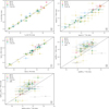 |
Fig. F.1 Comparison of our obtained parameters to literature values. a: Teff comparison, b: log g comparison, c: Lbol comparison, d: log |


Comparison of derived parameters to previous studies.
All Tables
List of the stars included in our analysis and the respective wavelength coverage.
Comparison of our adopted broadening parameters with those obtained via IACOB-BROAD (Simón-Díaz & Herrero 2014) applied to high-resolution MIKE data.
Slopes, x, and vertical offsets, log D0, of Equation (5) of this study and from Paper XIII.
All Figures
|
Fig. 1 Hertzsprung–Russell diagram for our sample. Overlaid in solid black lines are non-rotating SMC isochrones for different ages (≈0−10 Myr). Dashed black lines are the SMC rotating evolutionary tracks for stellar masses in the range of ≈10–60 M⊙ with a rotational velocity of 110 km s−1. Both the isochrones and evolutionary tracks are adopted from Brott et al. (2011). The shaded area is defined by the HD limit (Humphreys & Davidson 1979; Smith et al. 2004; Davies et al. 2018). |
| In the text | |
|
Fig. 2 Relative (percentage) difference of the evolutionary and spectroscopic masses (Mevo − Mspec)/Mspec. Mevo was obtained using a Bayesian inference method applied to SMC evolutionary models of Brott et al. (2011). The diagonal black crosses indicate the presence of a mass discrepancy. |
| In the text | |
|
Fig. 3 Best fits (solid red lines) to XShootU Hα (+ C ii λ6578) profiles (solid black lines). Magellan/MIKE spectra are also shown (dashed blue lines), where available, to illustrate line variability. |
| In the text | |
|
Fig. 4
|
| In the text | |
|
Fig. 5 v∞ vs Teff. The green dots represent our results. The green line is the linear fit. The dashed magenta line is the Z-dependent v∞–Teff relation from Hawcroft et al. (2024b). The solid magenta line was obtained from fitting Hawcroft et al. (2024b) results for O and B supergiants only. The solid blue line was obtained from fitting the results of Bernini-Peron et al. (2024). The grey crosses are v∞ calculated from Vink & Sander (2021) recipe. The black triangles represent v∞, calculated from the recipe in Krtička et al. (2021). |
| In the text | |
|
Fig. 6 ϵN vs vrot sin i. The colour scheme corresponds to the value of Γe. The solid pink, brown, orange, and red lines represent SMC evolutionary tracks for initial masses of 12 M⊙, 25 M⊙, 40 M⊙, and 60 M⊙, respectively, with initial rotational velocities of 110, 250, 350 km s−1 (Brott et al. 2011). We multiplied by a factor of π/4 to take into account the inclination of the rotation axis (Hunter et al. 2008). The dashed black line represents the baseline ϵN in the SMC (Vink et al. 2023). The dots along the evolutionary tracks represent time steps of 0.1 Myr. |
| In the text | |
|
Fig. 7 log N/C vs log N/O. The red triangles show the distribution of our sample. The stars for which the oxygen abundance was obtained from fitting the O i λλλ7772–7774–7775 multiplet are shown in blue squares. The dashed black lines represent the upper and lower boundaries adopted from Maeder et al. (2014). |
| In the text | |
|
Fig. 8 Dmom vs logLbol. The green symbols represent the SMC sample. The yellow symbols represent the LMC sample from Paper XIII. Circles indicate stars with reliable UV and optical wind diagnostics. Triangles indicate upper limits. Solid lines are fits to the circles. Dash-dotted lines are fits for the entire sample. |
| In the text | |
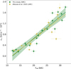 |
Fig. 9 v∞ vs Teff. The symbol and colour encoding are the same as in Fig. 8. |
| In the text | |
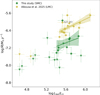 |
Fig. 10
|
| In the text | |
|
Fig. 11
|
| In the text | |
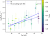 |
Fig. 12
|
| In the text | |
|
Fig. 13 Ratio (v∞/vesc) as a function of temperature. The solid green line represents the linear fit to our sample. The dashed black line is the relation presented in Krtička et al. (2021). The dotted red lines represent the ratios from Lamers et al. (1995). The colour gradient correlates with the value of Γe. |
| In the text | |
|
Fig. C.1 Wind efficiency |
| In the text | |
|
Fig. F.1 Comparison of our obtained parameters to literature values. a: Teff comparison, b: log g comparison, c: Lbol comparison, d: log |
| In the text | |
Current usage metrics show cumulative count of Article Views (full-text article views including HTML views, PDF and ePub downloads, according to the available data) and Abstracts Views on Vision4Press platform.
Data correspond to usage on the plateform after 2015. The current usage metrics is available 48-96 hours after online publication and is updated daily on week days.
Initial download of the metrics may take a while.