| Issue |
A&A
Volume 707, March 2026
|
|
|---|---|---|
| Article Number | A8 | |
| Number of page(s) | 13 | |
| Section | Stellar atmospheres | |
| DOI | https://doi.org/10.1051/0004-6361/202558211 | |
| Published online | 27 February 2026 | |
Dynamically consistent analysis of Galactic WN4b stars
Revised parameters and insights on Wolf–Rayet mass-loss treatments
1
Zentrum für Astronomie der Universität Heidelberg, Astronomisches Rechen-Institut,
Mönchhofstr. 12-14,
69120
Heidelberg,
Germany
2
Interdisziplinäres Zentrum für Wissenschaftliches Rechnen, Universität Heidelberg,
Im Neuenheimer Feld 225,
69120
Heidelberg,
Germany
3
Institute of Physics and Astronomy, University of Potsdam,
Karl-Liebknecht-Str. 24/25,
14476
Potsdam,
Germany
★ Corresponding author: This email address is being protected from spambots. You need JavaScript enabled to view it.
Received:
21
November
2025
Accepted:
8
January
2026
Abstract
Context. Many Wolf-Rayet (WR) stars have optically thick winds that essentially cloak the hydrostatic layers of the underlying star. In these cases, traditional spectral analysis methods are plagued by degeneracies that make it difficult to constrain parameters such as the stellar radius and the deeper density and velocity structure of the atmosphere.
Aims. Focussing on the regime of nitrogen-rich WN4 stars with strong emission lines, we employed hydrodynamically consistent modelling using the POWRHD code branch to perform a next-generation spectral analysis. The inherent coupling of the stellar and wind parameters enabled us to break parameter degeneracies, constrain the wind structure, and get a mass estimate. With this information, we were able to draw evolutionary implications and test current mass-loss descriptions for WR stars.
Methods. We selected a sample of six Galactic WN4b stars. Applying updated parallaxes from Gaia DR3 and calculating POWRHD models that sufficiently resemble most of their spectral appearance, we obtained new values for the stellar and wind parameters of the WN4b sample. We compared our results to previous studies employing grid models with a prescribed β = 1 velocity structure and cross-checked our derived parameters with stellar structure predictions from GENEC and FRANEC evolution tracks.
Results. For all six targets, we obtain a narrow range of stellar temperatures T* ~ 140 kK, in sharp contrast to previous grid-model analyses. We confirm the existence of WRs with luminosities as low as log L/L⊙ = 5.0 and M* ≈ 5 M⊙. All derived velocity fields include a plateau-like feature at ~85% of the terminal velocity. Both the distance updates and the switch to dynamically consistent atmospheres lead to substantial parameter adjustments compared to earlier grid-based studies. A comparison of the derived mass-loss rates favours a different description for the WN4b sample than for WN2 stars analysed with the same methodology.
Conclusions. WN4b winds are launched by the hot iron opacity bump, placing these hydrogen-free stars near or slightly hotter than the He zero age main sequence. Similar to a recent analysis of WN2 stars, we have thus solved the WR radius problem for the WN4b stars, but this conclusion cannot be extrapolated to regimes strongly affected by radiatively driven turbulence. Evolutionary models struggle to reproduce the empirical parameter combinations. The observed stars typically require lower mass loss in the current WR stage than predicted, but require further prior stripping in order to arrive at the observed stage.
Key words: stars: atmospheres / stars: early-type / stars: mass-loss / stars: winds, outflows / stars: Wolf-Rayet
© The Authors 2026
 Open Access article, published by EDP Sciences, under the terms of the Creative Commons Attribution License (https://creativecommons.org/licenses/by/4.0), which permits unrestricted use, distribution, and reproduction in any medium, provided the original work is properly cited.
This article is published in open access under the Subscribe to Open model. This email address is being protected from spambots. You need JavaScript enabled to view it. to support open access publication.
1 Introduction
In the domain of massive stars (stars with Minit ≳ 8 M⊙), Wolf-Rayet (WR) stars form a remarkable subgroup. Characterised by prominent emission lines in their spectra (e.g. Wolf & Rayet 1867; Beals 1940), WR stars show strong stellar winds emerging from the proximity to the Eddington limit, i.e. a mass-to-luminosity ratio (e.g. Gräfener & Hamann 2008; Sander et al. 2020). Most WR stars are found at the hottest and most luminous end of the Hertzsprung-Russell diagram (HRD). The combination of high temperature and luminosity along with a strong outflow causes these stars to be highly impactful. They serve as strong sources of ionising radiation (e.g. Smith et al. 2002; Sander 2022; Sander et al. 2025), contribute to local enrichment of their surroundings (e.g. Maeder 1983; Dray & Tout 2003; Farmer et al. 2021), and inject large amounts of kinetic energy into their surroundings via their stellar winds (e.g. Ramachandran et al. 2018). These winds lead to mass-loss rates of Ṁ ~ 10−5-10−3 M⊙ yr−1 and terminal velocities easily of the order of thousands of km s−1 (e.g. Crowther 2007). The powerful stellar wind heavily influences the WR star spectra, up to the point where the spectrum is completely dominated by wind lines (Hamann 1985; Davidson 1987; Hamann & Gräfener 2004). When the whole spectrum is formed in the rapidly expanding wind layers, the determination of the underlying stellar parameters becomes particularly challenging. The standard approach to analyse the spectra with an atmosphere model using the prescribed wind velocity field is limited by significant degeneracies (e.g. Hamann & Gräfener 2004; Lefever et al. 2023), in particular with respect to the (hydrostatic) stellar radius and its corresponding effective temperature. This limits the proper comparison with stellar structure and evolution models and has been termed the WR radius problem (e.g. Hillier 1987; Langer et al. 1988). This points towards the need for improvements in modelling techniques.
Most known WR stars are highly evolved objects. About 90% of all WR stars are in the helium burning stage (some may even be beyond), and thus are partially or completely depleted in hydrogen (e.g. van der Hucht 2001; Crowther 2007; Hainich et al. 2014; Shenar et al. 2019).
These classical WR (cWR) stars are further spectroscopically classified into WN stars with prominent nitrogen line presence, WC stars with strong carbon lines, and WO stars with strong oxygen lines (Hiltner & Schild 1966; Smith 1968). Transition types between WN and WC as well as WN and WO have been discovered (Massey & Grove 1989; Morris et al. 1996; Sander et al. 2025), which suggests an evolutionary connection (Gamow 1943) and implies that at least some WR stars are capable of intrinsically removing a sufficient part of their outer envelope to alter their surface abundances (Conti 1979; Conti et al. 1983). Further temperature classification has been done based on diagnostic line ratios within the three separate spectral classes (see Smith et al. 1996 for WN stars and Crowther et al. 1998 for WC and WO stars). A subgroup among the WN stars shows a notable presence of hydrogen at the surface, and are classified as WNh stars. These stars are compatible with corehydrogen burning massive stars close to the Eddington limit (e.g. de Koter et al. 1997; Crowther et al. 2010; Gräfener et al. 2011). However, the WNh classification can also be reached by incomplete stripping of the hydrogen envelope. This is more prominent at lower metallicity, in particular in the SMC where 11 out of the 12 known WR stars are of WNh type, but presumably all of them are He-burning (Hainich et al. 2015; Shenar et al. 2016).
In all of these separate classifications, the stellar wind determines the appearance of the objects with significant consequences for the spectral analysis. Given the aforementioned WR radius problem for WR stars with dense winds obtained in traditional studies (e.g. Hamann et al. 2006), the advent of dynamically consistent modelling for WR stars (e.g. Gräfener & Hamann 2005; Sander et al. 2020) offers a new opportunity to resolve this long-standing issue.
In this study, we focus on analysing Galactic dense-wind WR stars of the WN4 subtype, also labelled as WN4-s (Hamann et al. 1995) or WN4b (Smith et al. 1996) due to their strong, broad emission lines. All of our six sample stars (WR 1, WR6, WR7, WR 18, WR37, and the WN/WC star WR58) are known to be in the regime of parameter degeneracy in prior studies (Hamann et al. 2006; Sander et al. 2012). For this work we employed hydrodynamic consistency in our stellar atmosphere modelling (Gräfener & Hamann 2005; Sander et al. 2017) to obtain physically more accurate information about their parameters, in particular with respect to their hydrostatic radii and wind onset.
Our paper is organised as follows. The methodology of our analysis, along with details on how dynamic consistency is achieved, is laid out in Sect. 2. In Sect. 3, the key findings of our analysis are presented, with a special emphasis on the spectroscopic results, while also being put in the context of stellar evolution. Interwoven with the scientific results, the comparison with previous analyses, focussing on the differences due to the use of dynamically consistent wind modelling, is also provided in Sect. 3. The summary of this study’s main findings and future prospects is given in Sect. 4.
2 Methods and observational data
In order to accurately model WR star atmospheres, a number of processes need to be simulated simultaneously. The strong departure from local thermodynamic equilibrium (LTE) requires an extensive calculation of the population numbers from the equations of statistical equilibrium. This non-LTE calculation is interdependent with the radiation field, which is obtained by solving the radiative transfer in a comoving-frame approach to account for the expanding atmosphere. In addition, the (electron) temperature stratification needs to be determined, typically from radiative equilibrium, flux consistency, electron thermal balance, or a combination of these approaches. In this work, we use the PoWR stellar atmosphere code (Gräfener et al. 2002; Hamann & Gräfener 2003; Sander et al. 2015) to fulfill these tasks. Assuming spherical symmetry, PoWR in the standard version uses fixed input stellar and wind parameters (M, T*, R*, L, M, ν∞, β) to compute the stratifications of hot-star atmospheres and their emergent spectra. The wind hydrodynamics are approximated by a fixed υ(r), usually using a β velocity law, where υ(r) = υ∞(1 - R*/r)β (Castor et al. 1975). In the subsonic regime, this υ(r) is then smoothly attached to a hydrostatic solution (Sander et al. 2015). In the case of WR stars, often β = 1 is assumed (e.g. Hamann et al. 1988; Hillier & Miller 1999), in particular in the calculation of large model grids (e.g. Hamann & Gräfener 2004; Todt et al. 2015), but this value can be insufficient to accurately reflect the wind hydrodynamics and can lead to troublesome degeneracies (Gräfener & Hamann 2005; Sander et al. 2020; Lefever et al. 2023).
To overcome the limitations of the fixed-velocity approach, we therefore employed the PoWRHD branch Sander et al. (2017), which computes the velocity stratification by solving the hydrodynamic equation of motion
 (1)
(1)
throughout the atmosphere consistently. The left-hand side in Eq. (1) represents the repulsive forces, accelerating the wind (i.e. the gas pressure and the radiation forces), while on the right the attractive forces are written. The acceleration due to gas and turbulence pressure is denoted as apress while the radiative acceleration is termed arad. Solving Eq. (1) not only determines υ(r) and thus the terminal velocity υ∞, but the necessary boundary conditions (i.e. the conservation of the total optical depth in our case) also fix the mass-loss rate Ṁ to a unique value. For hot stars, these results for υ(r) and Ṁ are largely shaped by the strength and stratification of arad. In the subsonic region, the pressure term can be important as well. However, in the case of the studied cWR stars arad is significantly stronger than apress (see also Gräfener & Hamann 2005; Gräfener & Vink 2013).
In this work, we employed the PoWRHD branch to produce atmosphere models that resemble the spectral appearance of six Galactic WN4 stars while also reproducing the spectral energy distribution derived from photometry and flux-calibrated UV spectra. In addition to the direct implications of the updated treatment of the υ(r), we also included significantly more elements than in most earlier studies of WN4b stars to ensure a realistic calculation of the radiative force. An overview of these elements and their abundances can be found in Table A.1. The additional constraints between the stellar and wind parameters due to the hydrodynamic coupling considerably reduce the number of free parameters and thus also the room for fine-tuning the spectral appearance. For example, any adjustment of the clumping factor has direct implications for the terminal velocity and the mass-loss rate. As a consequence, the width of an emission line cannot be changed without also affecting the electron scattering wings. While this can limit the visual fit between observation and model, the higher physical consistency nonetheless marks a significant added value for the interpretation of the resulting best-matching model.
The observed UV, optical, and IR spectra we employed in this work were also used in previous analyses (Hamann et al. 2006; Sander et al. 2012). All UV spectra were taken by the International Ultraviolet Explorer (IUE). The optical and IR spectra originate from the European Southern Observatory (ESO), La Silla (Chile), from the Deutsch-Spanisches Astronomisches Zentrum (DSAZ) in Calar Alto (Spain), as well as from the Anglo-Australian Telescope (AAT) at Siding Spring (Australia). More detailed information for the optical and IR spectra of the six targets can also be found in Hamann et al. (1995). The optical narrow-band photometry data is from Lundstrom & Stenholm (1984). In addition, we employ the photometry from Gaia DR3 and (in the case of WR6) PAN-STARRS (Chambers et al. 2016). The IR broad-band photometry for our targets is taken from the 2MASS catalog (Skrutskie et al. 2006).
Five of the six targets studied in this work are not showing any signs of a luminous companion and thus have been analysed as single objects. Three of our sample stars are known for intrinsic variability, most notably WR6 (aka HD 50896 or EZCMa), which is sometimes interpreted as a possible companion signature (e.g. Dsilva et al. 2022). However, these variations are commonly interpreted as co-rotating interacting regions (CIRs), which were studied for several of our sample stars, namely WR 1 (St-Louis et al. 2009), WR 6 (St-Louis et al. 2018) and WR58 (Chené & St-Louis 2011). Additionally, three of our objects have a nebula associated with them: WR6, WR 7, and WR 18 with respectively Sh2-308, NGC 2359, and NGC 3199 as emission nebulae containing hot gas (Toalá et al. 2017; Camilloni et al. 2024). WR 18 has recently been investigated with VLTI/GRAVITY by Deshmukh et al. (2024), finding a diffuse component contributing to the K-band but no indication of binarity. We aimed for a spectral agreement of similar or improved quality over the previous analyses of our targets in Hamann et al. (2019, hereafter H19) and Sander et al. (2019, hereafter S19). As the spectra of all six targets are wind dominated, we used the option introduced in Sander et al. (2020) to fix the mass-loss rate and luminosity, while iterating over the stellar mass in the hydrodynamic iterations.
Given the interdependencies and the long calculation times, a high-dimensional parameter grid is computationally extremely expensive. Hence, the iteration in the parameter space was performed under manual supervision with the best-fit model chosen by visual inspection, similar to prior studies performed for the targets. The full visual comparisons can be seen in Appendix B for all six targets.
Selected parameters from the best-fit PoWRHD models of the six targets in this study.
3 Results and discussion
Using hydrodynamically consistent PoWRHD models (hereafter simply PoWRHD models), we were able to successfully replicate observed spectra for our six targets. For each target, the relevant parameters of the best-matching atmosphere models are shown in Table 1. The parameters of the previous analysis using a grid approach and β = 1 can be found in Table 1 from H19 for WR 1, WR6, WR7, WR18, and WR 37 and in Table 1 from S19 for WR58. The uncertainty values displayed in the figures of this study are based on the distance modulus (D.M.) uncertainties from Crowther et al. (2023), propagated via ε log10 L* = 0.4 ∙ εD.M., εlog10 R* = 0.2 ∙ εD.M., and εlog10 Ṁ = 0.3 ∙ εD.M. These latter three relations stem from the definition of the distance modulus D.M. = 5log10(d/10 pc) (with d the distance to the star), the Stefan-Boltzmann law (L* = 4π R*2 σSB T*4) and the transformed radius (see Eq. (2)).
3.1 Stellar parameter revision
There are substantial differences between the best-matching PoWRHD models and the previous analyses for all six targets. The older studies are based on assigning mainly grid models using β = 1 and contain significantly fewer elements than the current PoWRHD models; there is also updated parallax information due to the release of Gaia DR3. In this work, we used the new distances given in Crowther et al. (2023) and the corresponding online WR catalogue1 derived from the Gaia DR3 parallaxes including local zero point corrections by Lindegren et al. (2021) and Maíz Apellániz (2022). This results in considerable luminosity updates for some of the targets, mostly downwards as the previous parallaxes with higher uncertainties typically led to an overestimation of the distance. Together with the switch to PoWRHD models, significant position shifts in the HR diagram compared to H19 and S19 have been obtained as shown in Fig. 1. The figure shows a two-step shift: (1) the changes in L* solely due to the updated Gaia parallaxes and (2) the changes in both T*(τ = 20) and L* due to the different modelling we employed in this study. Here we note that, due to the updated distances, the Ṁ values of the H19 and S19 models are also affected (see e.g. Sect. 4 in H19). As evident from Table 1, the effective temperatures at the critical radius Tcrit are very similar to T*. This means that their winds must be launched rather deep as the radii corresponding to τ = 20 and the critical radius reflecting the wind onset are not very different. Moreover, the corresponding effective temperatures are now all very similar to ~ 140 kK and beyond the He-ZAMS line (Langer 1989). With the exception of WR58, the L* values on the other hand all decrease to various degrees when considering the new Gaia data. For comparison we also display the WN2 and WN/WO stars from Sander et al. (2025, hereafter S25) which have recently been analysed with the same methodology. With the exception of M31WR99-1, all S25 targets coalesce around a similar T*, albeit with a smaller spread in L*. We also note that both WR7 and WR58 have comparatively low luminosities for the bulk of WR stars and fall in the range of intermediate-mass stripped stars. The values we derive here are close to the (partially) stripped stars in Götberg et al. (2023) and Ramachandran et al. (2024) in the SMC, however, with significantly higher mass-loss rates.
While the PoWRHD models line up with very similar T* values in Fig. 1, a much wider range of temperatures was obtained in the grid analyses in H19 and S19. This was due to parameter degeneracies that limit constraining several stellar and wind parameters only to Ṁt ∝ Rt T2 (see also Eq. (2)) in the case of dense winds. This degeneracy can be broken with the PoWRHD modelling. As the wind structure is uniquely solved per atmosphere model, we can derive the effective temperature at the hydrostatic surface, for which we used the critical point as defined in Sander et al. (2017) as a reference radius. Moreover, as a specific set of wind parameters is coupled to a set of stellar parameters, it is not possible to change the emerging spectrum without changing the underlying stellar parameters, which provided us an indirect estimate of the otherwise inaccessible stellar mass. As hydrogen-free WN stars are close to the theoretical concept of a “helium star” (Langer 1989), our targets should be close to or slightly hotter than the He zero age main sequence (ZAMS). This is indeed the case when inspecting the Tcrit values for our WN4b sample as well as most of the S25 sample. Confirming the suggestions from the early WC prototype model by Gräfener & Hamann (2005), we can thus conclude that at least for WN2 and WN4b stars, hydrodynamically consistent atmosphere modelling is able to resolve the “WR radius problem”.
Notably, when considering the photospheric temperatures T2/3 = Teff(τ = 2/3) instead of T*, we obtained significantly smaller shifts in the HRD compared to the older studies as shown in Fig. 2, in particular along the temperature axis. This illustrates that for most of our targets the older models with β = 1 were reasonably sufficient in describing the layers from where the observed spectrum is emerging. We discuss this further in Sect. 3.2 when directly comparing the wind structures. When comparing Tcrit to Tτ=2/3 for the WN4b stars, i.e. the effective temperatures of the wind onset and of the emergent continuum, the difference is roughly a factor of two (cf. Table 1). This reflects how extended the atmospheres of the WN4b stars are, in sharp contrast to the PoWRHD results for the WN2 and WN/WO stars in S25, where the two temperatures are very similar. This is also evident from their position in the HRD (see Fig. 2), where the WN2 and WN/WO stars reside close to the He-ZAMS.
In terms of chemical abundance determination, the six targets do not deviate much from the bulk of Galactic WN stars. Initially using the abundances from the PoWR WN star model grids (Hamann & Gräfener 2004; Todt et al. 2015), with some small variations in the C and N abundances in order to assure certain spectral lines are modelled well. One such example is the case of the C IV λ5808Å line for WR58, shown in Fig. 5 in Appendix B, where an increased C abundance is crucial as WR58 is a known WN/WC star (van der Hucht 2001). For the other elements included in the wind modelling, where we have used solar abundances from Asplund et al. (2009), we refer to Table A.1 for the list of derived mass fractions and the modelled ions per element.
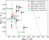 |
Fig. 1 HR diagram of the WN4b sample with parameters from H19 and S19 (black circles), updated parameters using only corrected parallaxes from Gaia DR3 (grey circles), and parameters from modelling with PoWRHD in this work (red). Gaia DR3 corrections are depicted by arrows from black circles to grey circles. Differences in addition to the distance corrections are illustrated with grey arrows from the grey circles to the red data points. For comparison, we also show the stars from S25 (cyan) as well as the H-ZAMS from Ekström et al. (2012) and the He-ZAMS from Langer (1989) as the grey and green dashed lines, respectively. |
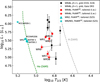 |
Fig. 2 Same as Fig. 1, but with the effective temperature T2/3 corresponding to an optical depth of τ = 2/3, on the x-axis. |
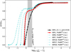 |
Fig. 3 Velocity stratification υ(r) comparison of the best-fit WN4b β = 1 grid model (H19, black connected circles) and the PoWRHD models in this work (red connected circles) of WR1. The υ(r) of the remaining five targets in this work are shown in cyan for comparison. The range of photospheric radii of the PoWRHD models at optical depth τ = 2/3 R2/3 is shaded in grey. The difference in outermost radii between the grid models and the PoWRHD models is due to the former being traditionally modelled up to 1000 R⊙ and the latter up to 50 000 R*. |
3.2 Wind structure comparison
In Fig. 3, we take a closer look at the velocity stratification for our six targets. In order to better compare the slopes, we scaled the velocities to the respective v∞ of the corresponding model. For comparison, we also show the old model for WR 1 from Hamann et al. (2006) and H19 using β = 1. In the outer wind, past 10 to 50R⊙, the slopes of the velocity laws essentially align with the β-law. However, in the inner wind, there is a significant deviation from a simple β-law as the velocity solutions from the PoWRHD models show a much steeper increase followed by a plateau or even a small decrease of the wind speed around v ≈ 0.85 v∞. Our obtained v(r)-stratifications generally align with the type of shape obtained for the fiducial early-type WN model presented in Sander et al. (2020). The ability to also yield non-monotonic solutions was later added in Sander et al. (2023) and is necessary for some of the targets here, for example WR 18 and WR 58. Note that the different total radial extension is only due to the different outer boundary choices in the modelling. While the traditional grid models were calculated up to 1000 R⊙, the PoWRHD models were calculated up to 50000 R*. This difference does, however, not significantly impact the resulting optical or UV spectra. Interestingly, the photospheric radii R2/3, i.e. the radii at optical depth τ = 2/3, coincide with the velocity stratification plateaus in the PoWRHD models. To first order, the remaining velocity field outwards of R2/3 can be described by a β-law, explaining the former success in the overall reproduction of the spectral features using β-law models. Moreover, it implies that there are still significant changes in the optically thin regime of the wind before v∞ is reached.
To understand the origin of the major differences in the inner wind, it is helpful to visualise the force balance for an exemplary hydro model and compare it to the situation in a β-type model. In Fig. 4, we depict the main acceleration and deceleration terms: gravity g and inertia amech slow down the wind material, while the pressure gradient ap and radiative acceleration arad push the wind outwards. The figure shows the total deceleration (g + amech) and the total acceleration (ap + arad) align for the PoWRHD model as hydrodynamic equilibrium is enforced. In contrast, the prescribed β-velocity law used in H19 and S19 does not account for the radiative acceleration in the inner wind due to the iron M-shell opacities. The location of R2/3 is marked in Fig. 4 as well, illustrating again that the spectra are formed outwards of this rapid inner acceleration and explaining why β-laws are yielding a reasonable spectrum despite the shortcomings in inferring the correct wind onset radii.
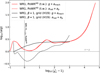 |
Fig. 4 Acceleration stratification comparison between the WN4b β = 1 grid model (H19, black lines) and the PoWRHD model (red lines) of WR1. The main wind deceleration terms (gravity g and wind inertia amech) are solid lines, while the main acceleration terms (radiative force arad and pressure gradient apress) are dashed lines. The grey horizontal line depicts the accelerations equal to gravity. The reason for the difference in outermost radii is the same as in Fig. 3. |
3.3 Mass-loss rates
The mass-loss rates Ṁ from the grid models in H19 and S19, and the PoWRHD models are shown in Fig. 5. In order to identify the influence of the different atmosphere modelling, we needed to separate again the correction resulting from the Gaia DR3 parallaxes applied to the older grid model solution. The classic WR model grids were calculated in two-dimensional planes spanning T* and the transformed radius,
 (2)
(2)
where D is the clumping factor. The definition of Rt stems from the early insight that models with varying Ṁ, R* and v∞ but the same Rt have very similar emission line equivalent widths (Schmutz et al. 1989). Due to the dependence on R* (and hence on L*), the mass-loss rates need to be scaled as well in order to keep Rt and thus the normalised spectrum when luminosities change due to updated parallaxes. As evident from Fig. 5, there is no systematic shift in Ṁ when shifting from the grid models to PoWRHD models. While WR1 shows hardly any changes at all, WR6, WR7, and WR58 show a significant decrease in Ṁ for our models. In some cases (e.g. WR18 and WR37, which have their Ṁ values increased compared to H19), the effect from the different modelling is contrary to the shift resulting from the updated distance.
With the updated mass-loss rates and the stellar parameters determined, we tested whether these combinations are predicted by commonly applied mass-loss recipes. In Fig. 6, we compare the descriptions by Nugis & Lamers (2000), the combined recipe by Yoon (2017, using fwr = 1.0), and the more recent formula from Sander & Vink (2020) to the values we determined for our six targets as well as to the stars from S25. With the exception of M31WR99-1, all of the targets have Tcrit ≈ 141 kK and thus we do not consider the temperature correction from Sander et al. (2023) when plotting the recipe curve (which would anyhow be target-dependent). In the uppermost panel of Fig. 6, we plot Ṁ versus L*/M*. The derived WN4b star parameters show quite some spread in this plane with larger uncertainties along the x-axis due to both L* and M* having inherent uncertainties. Notably, all stars are located above the line from Sander & Vink (2020) for solar metallicity. This is particularly interesting as the basic methodology to derive the recipe was the same, namely dynamically consistent modelling with PoWRHD. While some of the targets reach the curve within the uncertainties, others clearly do not. Sander & Vink (2020) assumed the mass-luminosity-relation from Gräfener et al. (2011) for their targets, which might not be the case for some of the WN4b stars. We examine this further below. Interestingly, the WN2 star WR 2 is precisely on the Sander & Vink (2020) curve for solar metal-licity. The other hotter WN and WN/WO stars are rightward of the curve, which is to be expected for subsolar metallicity. The WN/WO star M31WR99-1, as briefly mentioned above, is significantly off but is expected to have a weaker mass-loss rate due to its considerably hotter temperature.
The mass-loss recipes from Nugis & Lamers (2000) and Yoon (2017) do not have an L/M-dependence, but only an L-dependence. To still compare them in the M-L/M-plane, we use Eq. (5) from Nugis & Lamers (2000) to calculate the masses they would have assigned to those luminosities. In addition to altering the offset, their formula is taken from Schaerer & Maeder (1992) and thus based on stellar structure calculations. We applied the same relation also to the Yoon (2017) recipe in order to be able to compare their performance relative to each other. Interestingly, one half of the WN4b sample matches rather well with the calibrated Nugis & Lamers (2000) relation, while the other half stays above a factor of two in Ṁ below the curve. The second half of the sample is even overpredicted by the Yoon (2017) relation, although - for this limited sample - one could conclude that it provides a reasonable compromise. However, the relations fail for the sample of WN2 and WN/WO stars from S25 which have much lower mass-loss rates. Considering the BAT99 targets to have approximately 0.5 Z⊙, Yoon (2017) would predict a shift of the curve by about -0.18 dex in Ṁ due to Z0.6. The Z0.85 prediction from Vink & de Koter (2005) would yield -0.25 dex. Instead, downward shifts of about 0.7-0.8 dex would need to be applied to reach the derived locations in the Ṁ-L/M-plane. We can thus conclude that the empirically calibrated mass-loss recipes from both Yoon (2017, with fWR = 1.0) and Nugis & Lamers (2000) give reasonable results if the targets are similar to the bulk of the sample that was used to derive them. However, they struggle to predict the correct Ṁ for objects that are considerably different and comparatively rare. The theoretical/model-derived description can include such rare cases, but in turn struggles when objects are different from their basic assumptions.
Given that the recipes from Yoon (2017) and Nugis & Lamers (2000) explicitly only include an L-dependence and are also employed that way in many evolution calculations, we also compare our results in the M-L-plane (cf. middle panel of Fig. 6). In order to have the pure L* dependence for the Sander & Vink (2020) recipe, we employ Eq. (13) in Gräfener et al. (2011) to calculate stellar masses. For plotting the recipes, we assumed Y = 0.98 and Z = 0.014, in line with our empirical abundance determinations. Both Nugis & Lamers (2000) and Yoon (2017) do an excellent job in mapping the derived results although it seems that the empirical points hint at a less steep slope. Considering again the uppermost panel of Fig. 6 and the error margins, it is clear that all WN4b targets (and even WR 2) have very similar L/M ratios. As the stars have nearly the same Tcrit, one might say that an L-dependence is sufficient. However, the proximity to the Eddington Limit also needs to be accounted for, and thus an L-dependence has to be in addition to an L/M-dependence rather than instead.
In the bottom panel of Fig. 6, we now study the massluminosity plane, where we plot both the Gräfener et al. (2011) relation for hydrogen-free stars (inherent to the predictions from Sander & Vink 2020) and the Nugis & Lamers (2000) relation drawn from Schaerer & Maeder (1992). While the WN4b stars are close to the two curves, none of them is actually on the He-ZAMS relation from Gräfener et al. (2011). The lower mass stars in our sample (WR58 and WR7) show lower masses than expected for a star on the He-ZAMS, which could indicate that these stars are a bit further evolved than the rest of the sample. This effect can also be seen in the evolutionary tracks from Chieffi & Limongi (2013), which we plot for comparison and annotate with their respective initial masses and surface carbon mass fractions. Towards the end of core-He burning, the stars are predicted to get more luminous again. Yet, as we show in Sect. 3.5, this is usually obtained together with an increase in the temperature, which we do not observe. Nonetheless, the evolved interpretation would be in line by the fact that WR 7 and WR58 are located above the M(L/M) prediction for He-ZAMS-based models (middle panel of Fig. 6), while being “normal” with respect to Ṁt(L/M), which we discuss further below.
While lower masses for a given luminosity are expected from more evolved objects, the locations of WR 1 and WR 18 in the lower panel of Fig. 6 are indicating the opposite, namely an excess in mass compared to their luminosity, albeit with some uncertainty. As both stars have clearly no considerable amount of remaining hydrogen, the HeZAMS mass should be an upper limit for a given luminosity. One explanation could be an overestimation of the mass from the PoWRHD models, which Gonzàlez-Torà et al. (2025b) concluded when comparing PoWRHD models with 3D radiation-hydrodynamic models from Moens et al. (2022). In their study, this effect was of the order of 10% in the mass, which could be just enough to bring the targets back onto the Gräfener et al. (2011) curve. However, this would in turn also increase the luminosity excess for WR 58 and WR 7. Alternatively, our six targets could indicate that the L-M relation for hydrogen-free is actually a bit different from current structural predictions, but the small sample and the systematic uncertainties prevent us from drawing bigger conclusions here.
Finally, we compare the transformed mass-loss rate (defined in Gräfener & Vink 2013),
 (3)
(3)
which essentially represents the mass loss if the star had L* = 106 L⊙, υ∞ = 1000 km s−1 and D = 1. This quantity is a more elegant alternative to Rt and enables comparisons of objects with different luminosities. As this quantity does not change with distance updates when using grid models, the changes visualised in Fig. 7 reflect the necessary adjustments when transitioning from yβ-type models to PoWRHD models. Here, one needs to be aware that PoWRHD does no longer enable manual adjustments of υ∞ as this is an outcome of the basic stellar parameters and the wind solution. Therefore, the best-fit model is often a compromise where υ∞ is not perfectly tailored to the widths of emissions lines and P Cygni absorptions. Already from this effect, some variation in Ṁt compared to models where υ∞ is a free parameter is to be expected.
Sander & Vink (2020) found a linear trend of Ṁt versus L/M in the regime of optically thick winds with a Z-dependent breakdown when the winds eventually become optically thin. In Fig. 8, we show the derived positions of our sample stars compared to both the linear relation as well as tracks for specific metallici-ties arising from individual sets of models. Notably, WN4b stars align very well with the Ṁt prediction. WR 7 and WR 18 are shifted a bit downwards, which could indicate some issues with the derived parameters, but are still clearly in the dense-wind regime. In contrast, the WR sample from S25 shows optically thin winds and the locations in this diagram indicate that these stars might indeed have metallicities between LMC and SMC level - again with the exception of M31WR 99-1 which is clearly off, but also has a much higher Tcrit.
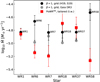 |
Fig. 5 Mass-loss rate Ṁ comparison between the WN4b β = 1 grid models (H19 & S19, black circles) and the PoWRHD models in this work (red squares). As in Figs. 1 and 2, the Gaia DR3 distance correction is applied on the grid models (grey circles) separate from the Ṁ updates in this work (see Sect. 3.3). The two-step parameter difference is denoted with the grey arrows per target. |
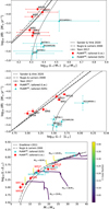 |
Fig. 6 Top panel: Ṁ values of the PoWRHD WN4b models in this work (red squares) and the S25 targets (cyan triangles) in terms of L*/M*. For comparison, the Ṁ laws from Nugis & Lamers (2000), Yoon (2017) and Sander & Vink (2020) are displayed. Middle panel: same Ṁ values, but in terms of L* and compared with the same predictions as in the top panel. Bottom panel: model L* values in terms of M*. The L* ~ M* relations from Nugis & Lamers (2000) and Gräfener et al. (2011) are shown as well, along with the evolutionary tracks (with rotation) from Chieffi & Limongi (2013) for initial masses 20, 30, 60, and 120 M⊙. The evolutionary tracks are colour-coded by carbon surface abundances in mass fractions. |
3.4 Ionising photon rates
As our WN4b stars have high effective temperatures and large luminosities, they are expected to be strong ionising sources. As illustrated in Fig. A.1, all of our targets are indeed strong sources of ionising photons beyond the hydrogen and He I ionisation edge. When comparing with the older analysis results, we see that the obtained changes are all in the direction of the adjustments in the luminosities of the targets due to the distance updates discussed above. A significant additional shift from the change to the PoWRHD models is only visible for targets that also had a further luminosity shift in the HRD (i.e. WR 1, WR7, and WR 37, cf. Fig. 1). This outlines that the difference in the velocity field and in particular the inner wind structure hardly affect these integrated quantities, implying that the common usage of ionising photon calculations from β-type atmosphere models in population synthesis is not a problem as such. However, our results also underline that the ionising photon production is not directly related to the hydrostatic radii of the stars. The expanding photospheres need to be taken into account, which is an open problem in current population synthesis modelling as the assignment of atmosphere models to predictions from evolutionary tracks is a highly non-trivial problem (see e.g. Groh et al. 2014; Josiek et al. 2025; Roy et al. 2025).
When inspecting the number of ionising photons beyond the He II edge, we obtained values of the order of only 1041 s−1, many orders of magnitude below what we obtain for QH and QHeI. This is not unexpected as the winds of all of our targets are so dense that these photons cannot escape. This is in stark contrast to the WN2 and WN/WO stars analysed in S25, where the QHe II values are comparable to the QHe I values of the WN4s here. In the model sequences calculated in Sander et al. (2023), a characterised transformed mass-loss rate of Ṁt ≈ 10−4.5 M⊙ yr−1 was found for the transition between WR stars that are opaque and transparent to He II ionising photons (see also González-Torà et al. 2025a). Indeed, our WN4b stars have Ṁt values considerably above this value while the WN2 and WN/WO stars from S25 show values below this limit. At least for the studied regime of WRs on or close to the He-ZAMS we can thus confirm the suitability of this value as a transition diagnostic.
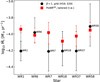 |
Fig. 7 Transformed mass-loss rates (Ṁt; see eq. (3)) of the WN4b β = 1 grid models (H19; S19, black circles) compared with the PoWRHD models in this work (red squares). The grey arrows denote the parameter difference between the two model sets. Here no distance correction as in Fig. 5 is required. |
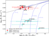 |
Fig. 8 Comparison of the WN4b PoWRHD models in this work (red squares), the S25 models (cyan triangles) in Ṁt-L*/M* space. In blue are the Ṁt tracks from Sander & Vink (2020) depicted for Z = 0.1, 0.2, 0.5 Z⊙ and Z = Z⊙. The thick gray dotted line indicates the fit in the dense-wind regime derived in Sander & Vink (2020). |
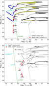 |
Fig. 9 HRD of the PoWRHD WN4b models (red squares), with the effective temperatures at the critical radius Tcrit (top panel). The GENEC evolutionary tracks without initial rotation from Ekström et al. (2012) with Mini = 40, 60, 85, and 120 M⊙ are shown, where we display effective temperatures not corrected for the wind. Separate segments of the evolutionary tracks are colour-coded by surface abundance: bold yellow denotes WNh stars (0.4 > XH > 0.02); bold black denotes WN stars (XH < 0.02); bold magenta denotes WN/WC stars (XC > 0.02); and bold blue denotes WC or WO stars (XC > 0.2). The tracks are further indicated in bold grey according to the criterion τ(R*) > 1.45 from Aguilera-Dena et al. (2022) (see also Eq. (4)). For comparison, the PoWRHD models of M31WR99-1 and WR2 from S25 are shown as well. The bottom panel shows the same PoWRHD models, but now comparing the wind-corrected temperatures given by GENEC with the determined T2/3 temperatures at τ = 2/3. In both panels the H-ZAMS from Ekström et al. (2012) and the He-ZAMS from Langer (1989) are shown as the grey and green dashed lines, respectively. |
3.5 Comparison with evolutionary tracks
While a detailed discussion about the origin of the WN4 stars easily warrants its own study, our derived HRD positions allow us to compare them to typical sets of published evolution tracks. Typically, evolution models add a simplified atmosphere on top of their structure that insufficiently corrects for the dense winds. Without a more sophisticated post-processing, the best way to compare our results is to take the effective temperature of the WN4b stars at the critical point Tcrit as this temperature essentially reflects the outmost radius that could be associated with a hydrostatic regime. This value is usually close to the effective temperature of the inner boundary T*, but as T* depends on the arbitrary choice of an associated (continuum) optical depth we prefer to use the more physical Tcrit.
3.5.1 Tracks without initial rotation
In Fig. 9, we compare our derived HRD locations with the sample of GENEC tracks from Ekström et al. (2012) which do not consider initial rotation. We show the tracks with Mini = 40, 60, 85 and 120 M⊙. In addition, the HRD of Fig. 2 is shown where the GENEC tracks are displayed with wind-corrected effective temperatures. For the WR stages, the GENEC models offer a distinct information of the effective temperatures without their otherwise inherent wind correction. We see that in principle our stars are now in a temperature regime where hydrogen-free WR stars are also predicted. However, the models with Mini < 40M⊙ do not evolve to the position in the HRD where WR stars are found and we therefore do not display these tracks. This means there are no tracks in this set which reach the derived HRD positions of WR6, WR7, and WR58. This remains true for the wind-corrected tracks in the bottom panel of Fig. 9. For WR 1, WR 18, and WR 37, there are suitable tracks leading to the obtained HRD positions, but they already predict WC surface abundances in this stage. Inspecting the corresponding masses from the track points, we get ~18.7 M⊙ from the Mini = 60 M⊙ track for WR 18. For WR37, the closest point is also on the Mini = 60 M⊙ track with a mass of ~14 M⊙ and for WR 1 this same track gives us ~15.6 M⊙. Compared to the masses we obtain with the spectral analysis (29.3 M⊙, 14.5 M⊙, and 19.6 M⊙ for WR 18, WR37, and WR 1, respectively), the evolutionary masses are systematically lower, albeit to varying degrees. This is the opposite to what is usually obtained for evolutionary masses of O stars. A recent comparison of the 1D PoWRHD models with 3D RHD simulations indicates that our approach might overestimate the stellar masses by ~ 10% (González-Torà et al. 2025b), but the difference is considerably larger than obtained in these benchmark calculations.
Given the predicted WC appearance, we checked whether the stripping during the WR stage itself in the GENEC model is too high. The 60 M⊙-track reaches the He-ZAMS with ~25 M⊙ and shows WC surface abundances approximately 70 000 years later with ~20 M⊙ left. This corresponds to an average massloss rate of 10−4.16 M⊙ yr−1, which is about a factor of four to five higher than what we obtain for the three more luminous WN4b stars. Considering the individual points of the stars, the mass-loss rates prescribed in the tracks are still typically a factor of 2.5 higher than we obtain. This implies that the time span of the hydrogen-free WN stage is likely underestimated in the tracks and that the predicted spectroscopic WN appearance is more extreme (i.e. stronger emission, cooler appearance) than empirically found. This likely also has impacts in the resulting kinetic feedback (e.g. Vieu et al. 2024; Hawcroft et al. 2025; Larkin et al. 2025) although studying one single WN subtype is too limited to draw broader conclusions. Moreover, despite the reasonable approximation of the Nugis & Lamers (2000) description in the Ṁ-L/M-plane, the L-dependent implementation, not just in GENEC but in stellar evolution tracks in general, seems to be problematic, even at solar metallicity. These specific conclusions of the inherent mass loss of hydrogen-free WNs on the He-ZAMS are largely independent of how the stars reached this HRD region and thus also remain valid for other stellar evolution codes and binary evolution calculations yielding WR stars.
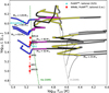 |
Fig. 10 Similar to Fig. 9, but the GENEC evolutionary tracks here are with an initial rotation of υini = 0.4 υcrit (Ekström et al. 2012). Here the evolutionary tracks with Mini = 32 and 25 M⊙ are also shown. |
3.5.2 Tracks with initial rotation
In Fig. 10, we consider the GENEC evolutionary models of stars which have an initial rotation velocity of 40% of the critical rotation, i.e. 3rot,ini = 0.4 3crit. Here, the picture shifts somewhat as models having a lower Mini can become WR stars, however they still fail to reach parameters similar to WR7 and WR58. WR 18 falls in between the Mini = 40 M⊙ and Mini = 60 M⊙ tracks here, where the closest points on the tracks respectively give ~15.7 M⊙ and ~19.0 M⊙. For WR 1 and WR 37 on the Mini = 40 M⊙ track, we get ~15.5 M⊙ and ~14.1 M⊙, respectively. With the rotating evolutionary models, the track with Mini = 32 M⊙ and the point with mass ~10.5 M⊙ can be representative for WR6 (having a spectroscopic mass of 10.3 M⊙). However, except for WR 6, the spectroscopic masses still tend to be significantly larger than the evolutionary ones from the tracks with initial rotation. Similarly, the discrepancy between the empirically obtained and the observed mass-loss rate remains. This is unsurprising as the implemented formula from Nugis & Lamers (2000) depends mainly on L and thus yields similar values for the same HRD position. Again, the match for WR 6 is the closest with a difference of 0.05 dex in log L and ~0.15 dex in Ṁ, albeit with a clear surface abundance mismatch.
As an alternative to the GENEC models, we also considered the FRANEC evolutionary tracks from Chieffi & Limongi (2013), where we make a similar comparison as with the GENEC tracks in Fig. 11. While the core principles of the codes are not as different as for example GENEC and MESA, the detailed treatment is sufficiently different to considerably affect the predicted evolution paths. The FRANEC models assume an initial rotational velocity of 300 km s−1 for all calculations rather than the fixed fraction of critical rotation assumed in GENEC. Moreover, the chemical mixing is less efficient (cf. Fig. 11 in Chieffi & Limongi 2013). Interestingly, the wind mass-loss treatment is roughly similar to GENEC with the main differences being in the exact treatment of the cool-star wind regime. The most noticeable difference between the GENEC and the FRANEC tracks is that the latter reach the He-ZAMS from initial masses as low as 20 M⊙. Thus, these tracks reach the positions of WR 6 and WR 7, predicting masses of 9.4 and 7.5 M⊙, respectively. This is within the uncertainty range of our obtained masses. For WR 1, WR 18, and WR37, the tracks predict ~15.7, ~20.0 and ~14.9 M⊙, very similar to the GENEC results. The predicted current mass-loss rates, however, are notably different. For WR 1, the predicted value of -4.9 is in line with the derived one, while for the much less luminous WR7, the predicted value of -5.5 is a factor of two too low. WR 6, which is intermediate in luminosity to the other two, is predicted to have -5.34, which is 0.24 dex too low. Again, also the surface abundances are off as all targets are predicted to have significant carbon surface abundances. While the WN/WC star WR 58 is not matched by the tracks, the prediction for the slightly more luminous WR7 is already XC ≈ 0.13 and XO ≈ 0.05, indicating too strong stripping of the WR star.
Given that both FRANEC and GENEC employ Nugis & Lamers (2000) for the WR stage, it is puzzling that they differ considerably in their Ṁ predictions. As their initial metallicity is very similar, the reason has to be a different implementation of the recipe. In GENEC, the original interpretation of Nugis & Lamers (2000) is used, where the whole sum of metals (Z) enters the calculation. In FRANEC, this might not be the case and just the initial metallicity is used. Then, the inherent, but not really physical Y-dependence (see e.g. the discussion in Higgins et al. 2021) would lead to a reduction in Ṁ if the tracks predict a C-enriched surface (i.e. Y ≲ 0.9), contrary to our findings (Y ≈ 0.98). Using Eq. (22) from Nugis & Lamers (2000) with this assumption approximately yields the FRANEC track values. However, the luminosity-dependent discrepancies remain. Moreover, while not scaling WR mass-loss rates with carbon is motivated by the findings of Vink & de Koter (2005) that even WC mass-loss rates mainly scale with iron, keeping the Hedependent term without changes is still problematic as it does not reflect the underlying physical effect, which is the difference in the free electron budget (Sander et al. 2020). Hence, it makes a difference whether He is lower due to H or C, but this is not mapped in the augmented Nugis & Lamers (2000) recipe.
Despite the success to reach the obtained HRD positions, significant caveats thus remain in explaining the evolutionary paths of WR stars. The agreement in mass-loss rates for targets such as WR 1 is due to coincidence rather than coherent treatment. Moreover, similar to the GENEC tracks, a high initial rotational velocity is required to have stars eventually reaching the hot side of the HRD in the FRANEC tracks. However, rotational velocities of around 300 km s−1 are rarely observed in the O-star regime. Holgado et al. (2022) determined rotational velocities of 285 O stars which are either single or dominated by the light of one component. Their obtained velocity distribution peaks at υ sin i < 100kms−1. Even when considering inclination effects, such stars would not rotate fast enough to be described by the FRANEC or GENEC tracks with rotation. While smaller secondary peaks exist around 200 and 300 km s−1 in Holgado et al. (2022), they are much smaller and seem to correlate more with binary-interaction products than objects undergoing unperturbed main sequence evolution. Therefore, the pathways to WR formation, in particular at the lower luminosity end, remain highly uncertain. Multiplicity might play an important role in this process, but also needs to explain why none of our sample stars show a luminous companion despite not being runaway stars. Compact companions are also unlikely as at least some WN4b stars such as WR 6 have been extensively monitored over decades.
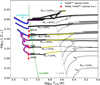 |
Fig. 11 Similar to Fig. 10, but for FRANEC evolutionary tracks (Chieffi & Limongi 2013) where the initial rotation has a value of vini = 300 km s−1. |
3.5.3 Wolf-Rayet identification
Traditionally, the WR phase and their different subtypes are identified by the surface abundances in stellar evolution models (e.g. Maeder 1991; Langer et al. 1994; Chen et al. 2015). We followed a similar scheme in the colouring of the tracks in Figs. 9 and 10. However, while the surface abundances might give a reasonable idea of whether we have a WNh, WN or WC/WO type, the abundances as such are not directly related to whether a star is sufficiently close to the Eddington Limit to have an emissionline spectrum and thus appear as a WR star (see e.g. Sander et al. 2020; Shenar et al. 2020). We thus also inspected the criterion from Langer (1989) to estimate the wind optical depth via
 (4)
(4)
where κe = 0.2 (1 - XH cm2 g−1) is the electron scattering opacity and υ0 is a velocity at the wind onset (Note that β = 1 is assumed to derive the above equation in Langer 1989). To obtain υ∞ for the evolution models, we use the expression  (with Γe denoting the Eddington factor for pure electron scattering) and assuming α ≈ 1.3 (see Gräfener et al. 2017). An optically thick wind can generally be defined by the wind optical depth surpassing unity. However, a proper definition would include the flux-weighted opacity including all contributions, in particular from line driving. To account for the simplifying assumptions in Eq. (4), Aguilera-Dena et al. (2022) attempted an observation-driven calibration, finding τ(R*) ≳ 1.45. Notably, this value is quite high, in particular as the electron scattering is only a fraction of the total opacity. Pauli et al. (2023) indeed only find τ(R*) ≳ 0.2 in order to match observations. Applying this τ(R*) ≳ 1.45 value to the evolutionary tracks in Figs. 9, 10, and 11, while assuming υ0 ≈ 20 km s−1, would essentially render the whole tracks as WR stars, which is clearly incorrect. In the above figures, we thus used the more conservative value of τ(R*) ≳ 1.45. Still, the outcome is that large parts of the depicted evolutionary tracks fulfils this criterion, while, with the exception of the very massive star (VMS) regime, this is neither observed nor intended from the calculations. For the switch to the VMS mass-loss regime, Sabhahit et al. (2022, 2023) suggest a formalism utilising the connection between the wind optical depth and the wind efficiency η = Ṁυ∞/(L/c). However, when calculating the wind efficiency for the tracks using the same, conservative assumption for υ∞, also almost all shown tracks from the main sequence on yield η > 1. Below the VMS regime, the main sequence should not fulfill this criterion, which is even above of what is actually required to switch on enhanced mass loss in Sabhahit et al. (2023). Hence, our tests essentially confirmed that the mass-loss rates in the OB main sequence regime are overestimated in the applied GENEC tracks.
4 Conclusions
By using hydrodynamically consistent atmosphere modelling with the PoWRHD branch, we successfully reproduced observed spectra of six Galactic WN4b stars and derived associated stellar and wind parameters, in combination with using updated Gaia DR3 parallaxes. Comparing the results of the models in this study with previous analyses in H19 & S19 that used grid models with a prescribed β = 1 velocity-law, we get substantial differences, even after correcting for influences from distance estimates (e.g. on L*, R* and Ṁ).
With the PoWRHD modelling approach, we reached a similar quality with synthetic spectrum, while also breaking previous degeneracies in the spectral analysis of our sample stars. Due to the solution of the wind hydrodynamics, the observed spectrum and its necessary mass-loss rate can only be reached with a much more compact solution than obtained in β-type modelling. All six WN4b targets have very similar effective temperatures at the critical radius, Tcrit ~ 140 kK; a value also representative of the stellar radius T* as the difference is quite small in our models (see Table 1). In contrast, prior analyses had the sample spread between T* ≈ 79 and 112 kK, though with the potential to also provide hotter solutions due to the spectrum fully emerging in the dense wind.
With their updated temperatures, the explored WN4 stars are now close or slightly hotter than the He-ZAMS. As none of our targets show signatures of hydrogen, such a location is expected from stellar structure modelling and we thus solve the long-standing WR radius problem, at least for the WN4b subtype. This finding aligns with the prototypical study by Gräfener & Hamann (2005) for the WC star WR 111 and the recent WN2 analysis by Sander et al. (2025), both also employing hydrodynamically consistent models. In all of these cases, the stellar wind is launched deeply at the hot iron bump created mainly by Fe M-shell opacities.
When comparing the updated mass-loss rates Ṁ with current predictions, we saw that the Sander & Vink (2020) M(L/M)-description systematically underpredicts M, while the transformed mass-loss rates Ṁt align well with predicted relations for the thick wind regime. As both works use essentially the same atmosphere modelling methodology, a major reason for this discrepancy is a difference between the mass-luminosity-relation inherent to Sander & Vink (2020) compared to what we found for our WN4b sample. As the same or similar relations were used in earlier studies to infer masses of WR stars, we conclude that stellar mass estimates from He-ZAMS-based relations such as Gräfener et al. (2011) will usually be too high, at least for strong-wind, early-type WR stars. This is notably different for the weaker-winded WN2 stars in Sander et al. (2025), which seem to closely align with a He-ZAMS relation.
When considering the mass-loss descriptions from Nugis & Lamers (2000) and Yoon (2017), which have an Ṁ(L)-type description, we conclude that both recipes perform well on average for the WN4b stars at Z ≈ 0.014. However, both recipes fail to reproduce the WN2 stars from Sander et al. (2025), while Sander & Vink (2020) does a reasonable job here and potentially could even offer an indirect metallicity diagnostic when the “breakdown regime” in Ṁ (cf. Sander & Vink 2020) is empirically mapped with WN2-like objects. Thus, we have to conclude that empirical recipes perform well if applied within the typical regime they were designed for, but have problems to cover more rare objects and suitably deal with lower metallicity.
Secondly, both GENEC and FRANEC models predict our WN4b stars to have a carbon-rich (i.e, WC- or WO-like) surface, which we can clearly rule out from our spectroscopic analysis. One of our objects, WR58, is of WN/WC-transition type, but the derived carbon abundance is way below the level of 1% typically expected for these transitions types. The inherent, unphysical dependencies on the current He- and Z-abundance in the Nugis & Lamers (2000) description lead to an overprediction of mass loss during the WR stage in the GENEC models. FRANEC seems to augment the recipe, resulting in an underprediction for lower luminosities. In cases where evolutionary tracks reach the derived HRD positions, there is a systematic difference on the stellar masses M*: for higher-luminosity objects, the mass derived from the PoWRHD modelling is higher than the mass from the tracks. For the lower-luminosity objects, the match is better, but tracks with a likely too high initial rotation need to be invoked.
The broader implications of our analysis and conclusions will have to be tested in future studies involving dense-wind Wolf-Rayet stars at different metallicity (e.g. in the LMC) as well as exploring more subtypes and wind density regimes. The solution of the WR radius problem for WN4b and WN2 stars is possible with the current modelling framework as both types of objects can be explained with winds that launch deep enough to not trigger larger amounts of radiation-driven turbulence. This is not the case for many other WR subtype configurations such as the weak-lined WN3 stars at lower metallicity (e.g. González-Torà et al. 2025a) which are located in a regime that cannot be explained by deep wind launching (e.g. Grassitelli et al. 2018; Sander et al. 2023) and will be significantly affected by turbulent pressure found in 3D and 2D simulations (Moens et al. 2022, 2025). To account for these, further developments in incorporating multi-D effects in 1D atmosphere modelling will be necessary. The mismatch to correctly represent or even reach the observed WR configurations with stellar evolution models further has significant effects on population synthesis, both in terms of stellar feedback as well as spectral predictions, and demands a deeper exploration of possible evolutionary pathways with updated physical treatments.
Data availability
Appendix B (spectral fits) and figures therein can be found in https://zenodo.org/records/18220388.
Acknowledgements
The authors would like to explicitly thank the anonymous referee for providing helpful comments that improved the quality of this document. The authors also want to thank R. Hirschi, G.N. Sabhahit, and J.S. Vink for inspiring discussions of some preliminary results that helped to outline the scope of this paper. R.R.L., A.A.C.S. and M.B.P. are supported by the Deutsche Forschungsgemeinschaft (DFG, German Research Foundation) in the form of an Emmy Noether Research Group - Project-ID 445674056 (SA4064/1-1, PI Sander). G.G.T. and J.J. are supported by the Deutsche Forschungsgemeinschaft (DFG, German Research Foundation) under Project-ID 496854903 (SA4064/2-1, PI Sander). G.G.T. and A.A.C.S. further acknowledge funding from the Federal Ministry for Economic Affairs and Climate Action (BMWK) via the Deutsches Zentrum für Luft- und Raumfahrt (DLR) grant 50 OR 2503 (PI Sander). V.R. acknowledges financial support by the Federal Ministry for Economic Affairs and Energy (BMWE) via the Deutsches Zentrum für Luft- und Raumfahrt (DLR) grant 50 OR 2509 (PI Sander). A.A.C.S., V.R., and E.C.S. further acknowledge financial support by the Federal Ministry for Economic Affairs and Climate Action (BMWK) via the German Aerospace Center (Deutsches Zentrum für Luft- und Raumfahrt, DLR) grant 50 OR 2306 (PI: Ramachan-dran/Sander). R.R.L., M.B.P., J.J. and E.C.S. are members of the International Max Planck Research School for Astronomy and Cosmic Physics at the University of Heidelberg (IMPRS-HD). This project was co-funded by the European Union (Project 101183150 - OCEANS).
References
- Aguilera-Dena, D. R., Langer, N., Antoniadis, J., et al. 2022, A&A, 661, A60 [NASA ADS] [CrossRef] [EDP Sciences] [Google Scholar]
- Asplund, M., Grevesse, N., Sauval, A. J., & Scott, P. 2009, ARA&A, 47, 481 [CrossRef] [Google Scholar]
- Beals, C. S. 1940, JRASC, 34, 169 [NASA ADS] [Google Scholar]
- Camilloni, F., Becker, W., & Sasaki, M. 2024, A&A, 681, A122 [NASA ADS] [CrossRef] [EDP Sciences] [Google Scholar]
- Castor, J. I., Abbott, D. C., & Klein, R. I. 1975, ApJ, 195, 157 [Google Scholar]
- Chambers, K. C., Magnier, E. A., Metcalfe, N., et al. 2016, arXiv e-prints [arXiv:1612.05560] [Google Scholar]
- Chen, Y., Bressan, A., Girardi, L., et al. 2015, MNRAS, 452, 1068 [Google Scholar]
- Chené, A.-N., & St-Louis, N. 2011, ApJ, 736, 140 [CrossRef] [Google Scholar]
- Chieffi, A., & Limongi, M. 2013, ApJ, 764, 21 [Google Scholar]
- Conti, P. S. 1979, in IAU Symposium, 83, Mass Loss and Evolution of O-Type Stars, eds. P. S. Conti & C. W. H. De Loore, 431 [Google Scholar]
- Conti, P. S., Garmany, C. D., De Loore, C., & Vanbeveren, D. 1983, ApJ, 274, 302 [NASA ADS] [CrossRef] [Google Scholar]
- Crowther, P. A. 2007, ARA&A, 45, 177 [Google Scholar]
- Crowther, P. A., De Marco, O., & Barlow, M. J. 1998, MNRAS, 296, 367 [NASA ADS] [CrossRef] [Google Scholar]
- Crowther, P. A., Schnurr, O., Hirschi, R., et al. 2010, MNRAS, 408, 731 [Google Scholar]
- Crowther, P. A., Rate, G., & Bestenlehner, J. M. 2023, MNRAS, 521, 585 [NASA ADS] [CrossRef] [Google Scholar]
- Davidson, K. 1987, ApJ, 317, 760 [NASA ADS] [CrossRef] [Google Scholar]
- de Koter, A., Heap, S. R., & Hubeny, I. 1997, ApJ, 477, 792 [Google Scholar]
- Deshmukh, K., Sana, H., Mérand, A., et al. 2024, A&A, 692, A109 [NASA ADS] [CrossRef] [EDP Sciences] [Google Scholar]
- Dray, L. M., & Tout, C. A. 2003, MNRAS, 341, 299 [Google Scholar]
- Dsilva, K., Shenar, T., Sana, H., & Marchant, P. 2022, A&A, 664, A93 [NASA ADS] [CrossRef] [EDP Sciences] [Google Scholar]
- Ekström, S., Georgy, C., Eggenberger, P., et al. 2012, A&A, 537, A146 [Google Scholar]
- Farmer, R., Laplace, E., de Mink, S. E., & Justham, S. 2021, ApJ, 923, 214 [NASA ADS] [CrossRef] [Google Scholar]
- Gamow, G. 1943, ApJ, 98, 500 [NASA ADS] [CrossRef] [Google Scholar]
- Georgy, C., Ekström, S., Meynet, G., et al. 2012, A&A, 542, A29 [NASA ADS] [CrossRef] [EDP Sciences] [Google Scholar]
- González-Torà, G., Sander, A. A. C., Egorova, E., et al. 2025a, A&A, 703, L11 [NASA ADS] [CrossRef] [EDP Sciences] [Google Scholar]
- González-Torà, G., Sander, A. A. C., Moens, N., et al. 2025b, A&A, 699, A244 [NASA ADS] [CrossRef] [EDP Sciences] [Google Scholar]
- Götberg, Y., Drout, M. R., Ji, A. P., et al. 2023, ApJ, 959, 125 [CrossRef] [Google Scholar]
- Gräfener, G., & Hamann, W. R. 2005, A&A, 432, 633 [NASA ADS] [CrossRef] [EDP Sciences] [Google Scholar]
- Gräfener, G., & Hamann, W.-R. 2008, A&A, 482, 945 [NASA ADS] [CrossRef] [EDP Sciences] [Google Scholar]
- Gräfener, G., & Vink, J. S. 2013, A&A, 560, A6 [NASA ADS] [CrossRef] [EDP Sciences] [Google Scholar]
- Gräfener, G., Koesterke, L., & Hamann, W.-R. 2002, A&A, 387, 244 [NASA ADS] [CrossRef] [EDP Sciences] [Google Scholar]
- Gräfener, G., Vink, J. S., de Koter, A., & Langer, N. 2011, A&A, 535, A56 [NASA ADS] [CrossRef] [EDP Sciences] [Google Scholar]
- Gräfener, G., Owocki, S. P., Grassitelli, L., & Langer, N. 2017, A&A, 608, A34 [NASA ADS] [CrossRef] [EDP Sciences] [Google Scholar]
- Grassitelli, L., Langer, N., Grin, N. J., et al. 2018, A&A, 614, A86 [NASA ADS] [CrossRef] [EDP Sciences] [Google Scholar]
- Groh, J. H., Meynet, G., Ekström, S., & Georgy, C. 2014, A&A, 564, A30 [NASA ADS] [CrossRef] [EDP Sciences] [Google Scholar]
- Hainich, R., Rühling, U., Todt, H., et al. 2014, A&A, 565, A27 [NASA ADS] [CrossRef] [EDP Sciences] [Google Scholar]
- Hainich, R., Pasemann, D., Todt, H., et al. 2015, A&A, 581, A21 [NASA ADS] [CrossRef] [EDP Sciences] [Google Scholar]
- Hamann, W. R. 1985, A&A, 148, 364 [Google Scholar]
- Hamann, W.-R., & Gräfener, G. 2003, A&A, 410, 993 [CrossRef] [EDP Sciences] [Google Scholar]
- Hamann, W.-R., & Gräfener, G. 2004, A&A, 427, 697 [NASA ADS] [CrossRef] [EDP Sciences] [Google Scholar]
- Hamann, W. R., Schmutz, W., & Wessolowski, U. 1988, A&A, 194, 190 [Google Scholar]
- Hamann, W.-R., Koesterke, L., & Wessolowski, U. 1995, A&A, 299, 151 [NASA ADS] [Google Scholar]
- Hamann, W.-R., Gräfener, G., & Liermann, A. 2006, A&A, 457, 1015 [NASA ADS] [CrossRef] [EDP Sciences] [Google Scholar]
- Hamann, W. R., Gräfener, G., Liermann, A., et al. 2019, A&A, 625, A57 [NASA ADS] [CrossRef] [EDP Sciences] [Google Scholar]
- Hawcroft, C., Leitherer, C., Aranguré, O., et al. 2025, ApJS, 280, 5 [Google Scholar]
- Higgins, E. R., Sander, A. A. C., Vink, J. S., & Hirschi, R. 2021, MNRAS, 505, 4874 [NASA ADS] [CrossRef] [Google Scholar]
- Hillier, D. J. 1987, ApJS, 63, 947 [NASA ADS] [CrossRef] [Google Scholar]
- Hillier, D. J. 1990, A&A, 231, 116 [NASA ADS] [Google Scholar]
- Hillier, D. J., & Miller, D. L. 1998, ApJ, 496, 407 [NASA ADS] [CrossRef] [Google Scholar]
- Hillier, D. J., & Miller, D. L. 1999, ApJ, 519, 354 [Google Scholar]
- Hillier, D. J., Lanz, T., Heap, S. R., et al. 2003, ApJ, 588, 1039 [Google Scholar]
- Hiltner, W. A., & Schild, R. E. 1966, ApJ, 143, 770 [NASA ADS] [CrossRef] [Google Scholar]
- Holgado, G., Simón-Díaz, S., Herrero, A., & Barbá, R. H. 2022, A&A, 665, A150 [NASA ADS] [CrossRef] [EDP Sciences] [Google Scholar]
- Josiek, J., Sander, A. A. C., Bernini-Peron, M., et al. 2025, A&A, 697, A193 [NASA ADS] [CrossRef] [EDP Sciences] [Google Scholar]
- Langer, N. 1989, A&A, 210, 93 [NASA ADS] [Google Scholar]
- Langer, N., Kiriakidis, M., El Eid, M. F., Fricke, K. J., & Weiss, A. 1988, A&A, 192, 177 [NASA ADS] [Google Scholar]
- Langer, N., Hamann, W.-R., Lennon, M., et al. 1994, A&A, 290, 819 [NASA ADS] [Google Scholar]
- Larkin, C. J. K., Hawcroft, C., Mackey, J., et al. 2025, A&A, 703, L14 [NASA ADS] [CrossRef] [EDP Sciences] [Google Scholar]
- Lefever, R. R., Sander, A. A. C., Shenar, T., et al. 2023, MNRAS, 521, 1374 [NASA ADS] [CrossRef] [Google Scholar]
- Lindegren, L., Bastian, U., Biermann, M., et al. 2021, A&A, 649, A4 [EDP Sciences] [Google Scholar]
- Lundstrom, I., & Stenholm, B. 1984, A&AS, 58, 163 [NASA ADS] [Google Scholar]
- Maeder, A. 1983, A&A, 120, 113 [NASA ADS] [Google Scholar]
- Maeder, A. 1991, A&A, 242, 93 [NASA ADS] [Google Scholar]
- Maíz Apellániz, J. 2022, A&A, 657, A130 [NASA ADS] [CrossRef] [EDP Sciences] [Google Scholar]
- Martins, F., Hillier, D. J., Bouret, J. C., et al. 2009, A&A, 495, 257 [NASA ADS] [CrossRef] [EDP Sciences] [Google Scholar]
- Massey, P., & Grove, K. 1989, ApJ, 344, 870 [Google Scholar]
- Moens, N., Poniatowski, L. G., Hennicker, L., et al. 2022, A&A, 665, A42 [NASA ADS] [CrossRef] [EDP Sciences] [Google Scholar]
- Moens, N., Debnath, D., Verhamme, O., et al. 2025, arXiv e-prints [arXiv:2511.04542] [Google Scholar]
- Morris, P. W., Eenens, P. R. J., Hanson, M. M., Conti, P. S., & Blum, R. D. 1996, ApJ, 470, 597 [Google Scholar]
- Nugis, T., & Lamers, H. J. G. L. M. 2000, A&A, 360, 227 [NASA ADS] [Google Scholar]
- Pauli, D., Oskinova, L. M., Hamann, W.-R., et al. 2023, A&A, 673, A40 [NASA ADS] [CrossRef] [EDP Sciences] [Google Scholar]
- Ramachandran, V., Hamann, W. R., Hainich, R., et al. 2018, A&A, 615, A40 [NASA ADS] [CrossRef] [EDP Sciences] [Google Scholar]
- Ramachandran, V., Sander, A. A. C., Pauli, D., et al. 2024, A&A, 692, A90 [NASA ADS] [CrossRef] [EDP Sciences] [Google Scholar]
- Roy, A., Krumholz, M. R., Salvadori, S., et al. 2025, A&A, 696, A29 [NASA ADS] [CrossRef] [EDP Sciences] [Google Scholar]
- Sabhahit, G. N., Vink, J. S., Higgins, E. R., & Sander, A. A. C. 2022, MNRAS, 514, 3736 [NASA ADS] [CrossRef] [Google Scholar]
- Sabhahit, G. N., Vink, J. S., Sander, A. A. C., & Higgins, E. R. 2023, MNRAS, 524, 1529 [NASA ADS] [CrossRef] [Google Scholar]
- Sander, A., Hamann, W.-R., & Todt, H. 2012, A&A, 540, A144 [NASA ADS] [CrossRef] [EDP Sciences] [Google Scholar]
- Sander, A., Shenar, T., Hainich, R., et al. 2015, A&A, 577, A13 [NASA ADS] [CrossRef] [EDP Sciences] [Google Scholar]
- Sander, A. A. C. 2022, arXiv e-prints [arXiv:2211.05424] [Google Scholar]
- Sander, A. A. C., & Vink, J. S. 2020, MNRAS, 499, 873 [Google Scholar]
- Sander, A. A. C., Hamann, W. R., Todt, H., Hainich, R., & Shenar, T. 2017, A&A, 603, A86 [NASA ADS] [CrossRef] [EDP Sciences] [Google Scholar]
- Sander, A. A. C., Hamann, W. R., Todt, H., et al. 2019, A&A, 621, A92 [NASA ADS] [CrossRef] [EDP Sciences] [Google Scholar]
- Sander, A. A. C., Vink, J. S., & Hamann, W.-R. 2020, MNRAS, 491, 4406 [Google Scholar]
- Sander, A. A. C., Lefever, R. R., Poniatowski, L. G., et al. 2023, A&A, 670, A83 [NASA ADS] [CrossRef] [EDP Sciences] [Google Scholar]
- Sander, A. A. C., Lefever, R. R., Josiek, J., et al. 2025, Nat. Astron., [arXiv:2508.18410] [Google Scholar]
- Santolaya-Rey, A. E., Puls, J., & Herrero, A. 1997, A&A, 323, 488 [NASA ADS] [Google Scholar]
- Schaerer, D., & Maeder, A. 1992, A&A, 263, 129 [NASA ADS] [Google Scholar]
- Schmutz, W., Hamann, W.-R., & Wessolowski, U. 1989, A&A, 210, 236 [NASA ADS] [Google Scholar]
- Scott, P., Asplund, M., Grevesse, N., Bergemann, M., & Sauval, A. J. 2015a, A&A, 573, A26 [NASA ADS] [CrossRef] [EDP Sciences] [Google Scholar]
- Scott, P., Grevesse, N., Asplund, M., et al. 2015b, A&A, 573, A25 [NASA ADS] [CrossRef] [EDP Sciences] [Google Scholar]
- Shenar, T., Hainich, R., Todt, H., et al. 2016, A&A, 591, A22 [NASA ADS] [CrossRef] [EDP Sciences] [Google Scholar]
- Shenar, T., Sablowski, D. P., Hainich, R., et al. 2019, A&A, 627, A151 [NASA ADS] [CrossRef] [EDP Sciences] [Google Scholar]
- Shenar, T., Gilkis, A., Vink, J. S., Sana, H., & Sander, A. A. C. 2020, A&A, 634, A79 [NASA ADS] [CrossRef] [EDP Sciences] [Google Scholar]
- Skrutskie, M. F., Cutri, R. M., Stiening, R., et al. 2006, AJ, 131, 1163 [NASA ADS] [CrossRef] [Google Scholar]
- Smith, L. F. 1968, MNRAS, 138, 109 [NASA ADS] [CrossRef] [Google Scholar]
- Smith, L. F., Shara, M. M., & Moffat, A. F. J. 1996, MNRAS, 281, 163 [NASA ADS] [CrossRef] [Google Scholar]
- Smith, L. J., Norris, R. P. F., & Crowther, P. A. 2002, MNRAS, 337, 1309 [CrossRef] [Google Scholar]
- St-Louis, N., Chené, A.-N., Schnurr, O., & Nicol, M.-H. 2009, ApJ, 698, 1951 [NASA ADS] [CrossRef] [Google Scholar]
- St-Louis, N., Tremblay, P., & Ignace, R. 2018, MNRAS, 474, 1886 [Google Scholar]
- Toalá, J. A., Marston, A. P., Guerrero, M. A., Chu, Y.-H., & Gruendl, R. A. 2017, ApJ, 846, 76 [CrossRef] [Google Scholar]
- Todt, H., Sander, A., Hainich, R., et al. 2015, A&A, 579, A75 [NASA ADS] [CrossRef] [EDP Sciences] [Google Scholar]
- van der Hucht, K. A. 2001, New A Rev., 45, 135 [CrossRef] [Google Scholar]
- Vieu, T., Larkin, C. J. K., Härer, L., et al. 2024, MNRAS, 532, 2174 [NASA ADS] [CrossRef] [Google Scholar]
- Vink, J. S., & de Koter, A. 2005, A&A, 442, 587 [NASA ADS] [CrossRef] [EDP Sciences] [Google Scholar]
- Wolf, C. J. E., & Rayet, G. 1867, Acad. Sci. Paris Comptes Rendus, 65, 292 [Google Scholar]
- Yoon, S.-C. 2017, MNRAS, 470, 3970 [NASA ADS] [CrossRef] [Google Scholar]
Appendix A Ionising fluxes, abundances, and modelled elemental ions
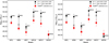 |
Fig. A.1 Amount of ionising photons for HI (QHI, left panel) and for He I (QHI, right panel) in the case of the β = 1 grid models (H19 & S19, black circles) and the PoWRHD models (red squares). Similar to Figs. 1, 2, and 5, a correction for GAIA DR3 parallaxes (grey circles) was made in order to separate the effects of distance updates and model differences, denoted by the grey arrows. |
Elements, mass fractions Xm, and ions used for the PoWRHD models in this worka.
All Tables
Selected parameters from the best-fit PoWRHD models of the six targets in this study.
Elements, mass fractions Xm, and ions used for the PoWRHD models in this worka.
All Figures
|
Fig. 1 HR diagram of the WN4b sample with parameters from H19 and S19 (black circles), updated parameters using only corrected parallaxes from Gaia DR3 (grey circles), and parameters from modelling with PoWRHD in this work (red). Gaia DR3 corrections are depicted by arrows from black circles to grey circles. Differences in addition to the distance corrections are illustrated with grey arrows from the grey circles to the red data points. For comparison, we also show the stars from S25 (cyan) as well as the H-ZAMS from Ekström et al. (2012) and the He-ZAMS from Langer (1989) as the grey and green dashed lines, respectively. |
| In the text | |
|
Fig. 2 Same as Fig. 1, but with the effective temperature T2/3 corresponding to an optical depth of τ = 2/3, on the x-axis. |
| In the text | |
|
Fig. 3 Velocity stratification υ(r) comparison of the best-fit WN4b β = 1 grid model (H19, black connected circles) and the PoWRHD models in this work (red connected circles) of WR1. The υ(r) of the remaining five targets in this work are shown in cyan for comparison. The range of photospheric radii of the PoWRHD models at optical depth τ = 2/3 R2/3 is shaded in grey. The difference in outermost radii between the grid models and the PoWRHD models is due to the former being traditionally modelled up to 1000 R⊙ and the latter up to 50 000 R*. |
| In the text | |
|
Fig. 4 Acceleration stratification comparison between the WN4b β = 1 grid model (H19, black lines) and the PoWRHD model (red lines) of WR1. The main wind deceleration terms (gravity g and wind inertia amech) are solid lines, while the main acceleration terms (radiative force arad and pressure gradient apress) are dashed lines. The grey horizontal line depicts the accelerations equal to gravity. The reason for the difference in outermost radii is the same as in Fig. 3. |
| In the text | |
|
Fig. 5 Mass-loss rate Ṁ comparison between the WN4b β = 1 grid models (H19 & S19, black circles) and the PoWRHD models in this work (red squares). As in Figs. 1 and 2, the Gaia DR3 distance correction is applied on the grid models (grey circles) separate from the Ṁ updates in this work (see Sect. 3.3). The two-step parameter difference is denoted with the grey arrows per target. |
| In the text | |
|
Fig. 6 Top panel: Ṁ values of the PoWRHD WN4b models in this work (red squares) and the S25 targets (cyan triangles) in terms of L*/M*. For comparison, the Ṁ laws from Nugis & Lamers (2000), Yoon (2017) and Sander & Vink (2020) are displayed. Middle panel: same Ṁ values, but in terms of L* and compared with the same predictions as in the top panel. Bottom panel: model L* values in terms of M*. The L* ~ M* relations from Nugis & Lamers (2000) and Gräfener et al. (2011) are shown as well, along with the evolutionary tracks (with rotation) from Chieffi & Limongi (2013) for initial masses 20, 30, 60, and 120 M⊙. The evolutionary tracks are colour-coded by carbon surface abundances in mass fractions. |
| In the text | |
|
Fig. 7 Transformed mass-loss rates (Ṁt; see eq. (3)) of the WN4b β = 1 grid models (H19; S19, black circles) compared with the PoWRHD models in this work (red squares). The grey arrows denote the parameter difference between the two model sets. Here no distance correction as in Fig. 5 is required. |
| In the text | |
|
Fig. 8 Comparison of the WN4b PoWRHD models in this work (red squares), the S25 models (cyan triangles) in Ṁt-L*/M* space. In blue are the Ṁt tracks from Sander & Vink (2020) depicted for Z = 0.1, 0.2, 0.5 Z⊙ and Z = Z⊙. The thick gray dotted line indicates the fit in the dense-wind regime derived in Sander & Vink (2020). |
| In the text | |
|
Fig. 9 HRD of the PoWRHD WN4b models (red squares), with the effective temperatures at the critical radius Tcrit (top panel). The GENEC evolutionary tracks without initial rotation from Ekström et al. (2012) with Mini = 40, 60, 85, and 120 M⊙ are shown, where we display effective temperatures not corrected for the wind. Separate segments of the evolutionary tracks are colour-coded by surface abundance: bold yellow denotes WNh stars (0.4 > XH > 0.02); bold black denotes WN stars (XH < 0.02); bold magenta denotes WN/WC stars (XC > 0.02); and bold blue denotes WC or WO stars (XC > 0.2). The tracks are further indicated in bold grey according to the criterion τ(R*) > 1.45 from Aguilera-Dena et al. (2022) (see also Eq. (4)). For comparison, the PoWRHD models of M31WR99-1 and WR2 from S25 are shown as well. The bottom panel shows the same PoWRHD models, but now comparing the wind-corrected temperatures given by GENEC with the determined T2/3 temperatures at τ = 2/3. In both panels the H-ZAMS from Ekström et al. (2012) and the He-ZAMS from Langer (1989) are shown as the grey and green dashed lines, respectively. |
| In the text | |
|
Fig. 10 Similar to Fig. 9, but the GENEC evolutionary tracks here are with an initial rotation of υini = 0.4 υcrit (Ekström et al. 2012). Here the evolutionary tracks with Mini = 32 and 25 M⊙ are also shown. |
| In the text | |
|
Fig. 11 Similar to Fig. 10, but for FRANEC evolutionary tracks (Chieffi & Limongi 2013) where the initial rotation has a value of vini = 300 km s−1. |
| In the text | |
|
Fig. A.1 Amount of ionising photons for HI (QHI, left panel) and for He I (QHI, right panel) in the case of the β = 1 grid models (H19 & S19, black circles) and the PoWRHD models (red squares). Similar to Figs. 1, 2, and 5, a correction for GAIA DR3 parallaxes (grey circles) was made in order to separate the effects of distance updates and model differences, denoted by the grey arrows. |
| In the text | |
Current usage metrics show cumulative count of Article Views (full-text article views including HTML views, PDF and ePub downloads, according to the available data) and Abstracts Views on Vision4Press platform.
Data correspond to usage on the plateform after 2015. The current usage metrics is available 48-96 hours after online publication and is updated daily on week days.
Initial download of the metrics may take a while.