| Issue |
A&A
Volume 707, March 2026
|
|
|---|---|---|
| Article Number | L5 | |
| Number of page(s) | 7 | |
| Section | Letters to the Editor | |
| DOI | https://doi.org/10.1051/0004-6361/202558457 | |
| Published online | 26 February 2026 | |
Letter to the Editor
Data-driven magnetohydrodynamic simulation of the initiation of a coronal mass ejection with multiple stages
1
Centre for Mathematical Plasma Astrophysics, Department of Mathematics, KU Leuven Celestijnenlaan 200B B-3001 Leuven, Belgium
2
School of Astronomy and Space Science, Nanjing University Nanjing 210046, People’s Republic of China
3
Institute of Physics, University of Maria Curie-Skłodowska Pl. Marii Curie-Skłodowskiej 5 20-031 Lublin, Poland
4
LIRA, Observatoire de Paris, CNRS, UPMC, Université Paris Diderot 5 place Jules Janssen 92190 Meudon, France
5
LUNEX EMMESI Institut, SBIC Kapteyn straat 1 Noordwijk 2201 BB, The Netherlands
★ Corresponding author: This email address is being protected from spambots. You need JavaScript enabled to view it.
Received:
8
December
2025
Accepted:
9
February
2026
Abstract
Coronal mass ejections (CMEs) are the primary drivers of adverse space-weather events, yet their initiation and onset prediction remain insufficiently understood due to the complexity of the magnetic topology and physical processes in real solar source regions. Using a fully observational-data-driven magnetohydrodynamic simulation, we successfully reproduced the initiation of a CME originating from the super active region 13663, with only a one-minute time lag between the flare peak in observations and the velocity peak of the rising flux rope in the simulation. Moreover, the eruptive structure exhibits a multi-stage kinematic evolution: an initial slow acceleration, a plateau at a nearly stationary height, and a subsequent impulsive acceleration. These stages correspond to torus instability, the downward tension force exerted by the overlying toroidal field, and fast magnetic reconnection, respectively. Our results highlight the inherently multistage nature of CME initiation in real events. In configurations with strong overlying toroidal fields, the downward toroidal-field-induced tension force can suppress the rise of the flux rope and produce a plateau phase at a nearly stable height, even when torus instability occurs. In contrast, the subsequent fast magnetic reconnection beneath the flux rope can drive the impulsive eruption more effectively. The close agreement between the observed and simulated peak times over one minute demonstrates the strong potential of our data-driven model for predicting CME onset.
Key words: Sun: coronal mass ejections (CMEs)
© The Authors 2026
 Open Access article, published by EDP Sciences, under the terms of the Creative Commons Attribution License (https://creativecommons.org/licenses/by/4.0), which permits unrestricted use, distribution, and reproduction in any medium, provided the original work is properly cited.
This article is published in open access under the Subscribe to Open model. This email address is being protected from spambots. You need JavaScript enabled to view it. to support open access publication.
1. Introduction
Coronal mass ejections (CMEs) are large-scale expulsions of magnetized plasma from the solar corona into interplanetary space and constitute the largest eruptive events currently known in the Solar System (Chen 2011; Webb & Howard 2012; Schmieder et al. 2015). Moreover, CMEs are considered the primary drivers of adverse space-weather events, such as geomagnetic storms, which can potentially impact satellite operations and communication and navigation systems (Gosling 1993; Schrijver et al. 2015). Consequently, understanding how CMEs are initiated and evolve in the low corona is essential to improving space-weather forecasting capabilities.
The early-stage kinematics of CMEs are commonly described in terms of a quasi-static phase (Xing et al. 2018), a slow-rise phase (Cheng et al. 2020), and an impulsive phase (Zhang et al. 2001; Zhang & Dere 2006). The quasi-static and slow-rise phases prior to eruption can be explained by the formation of a current sheet and the response of driving flows (Xing et al. 2024b; Liu et al. 2025), with moderate reconnection occurring at the hyperbolic flux tube (Titov et al. 2002) beneath the flux rope (Cheng et al. 2023; Xing et al. 2024a). The impulsive phase, characterized by the onset of rapid CME acceleration, can be triggered by several mechanisms, for example torus instability (TI; Kliem & Török 2006; Aulanier et al. 2010), fast tether-cutting magnetic reconnection below the flux rope (Jiang et al. 2021), and breakout reconnection above it (Antiochos et al. 1999). These models establish a basic physical framework for understanding how a CME develops and ultimately erupts.
Although these models capture several key physical processes involved in CME initiation (before and at the impulsive phase), their application to forecasting real solar eruptions remains highly challenging. This is because they are based on simplified magnetic configurations (e.g., bipoles or quadrupoles) and on idealized driving flows (e.g., shearing or converging motions), which differ significantly from the conditions in real active regions (ARs). The evolution of real ARs involves the interplay of shearing and converging flows, magnetic flux emergence (Chen & Shibata 2000; Fan 2018), and collisional shearing motions between different magnetic systems (Chintzoglou et al. 2019), which leads to highly complex and twisted magnetic topologies. As a result, CME kinematics presented in the literature are often multi-staged and highly variable, making real-time CME forecasting particularly difficult.
Observational data-driven simulations have recently been developed and have become essential tools for studying CME initiation and forecasting their onset (Jiang et al. 2022). Using our recently developed data-driven magnetohydrodynamic (MHD) model (Guo et al. 2019; Zhong et al. 2023; Guo et al. 2024a), we investigated the initiation of a CME in the super AR 13663, which produced more than 20 M-class or higher solar flares within six days. This study had two main objectives. First, we aimed to assess the capability of our data-driven model to forecast real and complex solar eruptions. Second, we explored the CME onset, which is highly complex in reality and often exhibits multiple stages, and we discuss the roles of TI and magnetic reconnection. Section 2 presents an overview of observations and describes the numerical model. In Sect. 3 we present the simulation results. This is followed by a summary and concluding remarks in Sect. 4.
2. Overview of observations and modeling
NOAA AR 13663 is classified as a Hale-βγδ class AR and has produced more than 20 intense flares and CMEs (Schmieder et al. 2025; Lekshmi et al. 2025). Interactions between CMEs originating from ARs 13663 and 13664 subsequently induced a major geomagnetic storm, with a peak Dst of –412 nT. In this Letter, we focus on the X1.3 flare and its associated CME initiation that occurred at approximately 06:00 UT on 2024 May 5.
As shown in Fig. 1a, three flares were detected by the GOES, as indicated by the soft X-ray light curve between 04:00 and 08:00 UT, including two confined C8.4 and C5.5 flares at ∼04:20 UT and ∼05:25 UT and an eruptive X1.3 flare with an associated faint CME at ∼05:47 UT. Figures 1b–d present composite Solar Dynamics Observatory (SDO, Pesnell et al. 2012)/Atmospheric Imaging Assembly (AIA, Lemen et al. 2012) 304 and 131 Å images at the peak moments of the three flares, while Figs. 1e and 1f display the corresponding 1600 Å flare ribbons. The eruptive flare exhibits multiple elongated and circular ribbon structures, indicating that the magnetic topology of this AR is highly complex. Figure 1g shows the 3D magnetic fields at 05:00 UT, from which one can observe a twisted flux rope, fan-spine structure, and overlying coronal loops, resembling the observations. Appendix A introduces the numerical setup.
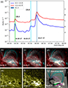 |
Fig. 1. Panel (a): Soft X-ray light curves (red: 1–8 Å; blue: 0.5–4 Å) from 04:00 to 08:00 UT on 2024 May 5. The vertical green, sky-blue, and dark blue lines mark the confined C8.4 and C5.5 flares and the eruptive X1.3 flare, respectively. Panels (b)–(d): Composite SDO/AIA 304 Å (red) and 131 Å (blue) images at the peak times of the three flares. Panels (e) and (f): 1600 Å flare-ribbon morphology of the first confined flare and the third eruptive flare, respectively. Panel (g): 3D magnetic field configuration from the data-driven MHD model at 05:00 UT. The green, pink, and cyan lines represent the flux rope, the fan–spine structure, and the surrounding coronal loops, respectively. |
3. Results
Figure 2 shows the global evolution of the 3D magnetic field before and during the CME initiation, from which we can see the formation and eruption of a twisted magnetic flux rope. At 04:22 UT (panels a–b), the coronal magnetic field is dominated by highly sheared arcades above the polarity inversion line. As the driving flows persist, a twisted flux rope forms at about 04:46 UT. Thereafter, the flux rope continues to accumulate twist and slowly rises. After 05:40 UT, it undergoes rapid expansion and upward acceleration, and the magnetic system transitions into the eruptive phase at about 05:46 UT. During this stage, the magnetic-field strength of the flux rope decreases significantly, and it develops into a large-scale, strongly twisted structure that ultimately drives the CME. Notably, the CME flux rope in the simulation leans toward the northeast, consistent with the CME trajectory observed near the solar north pole. Moreover, the starting time of the impulsive eruption of the flux rope is nearly the peak time of the X1.3 flare.
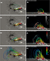 |
Fig. 2. Evolution of the 3D magnetic field lines in the simulation. The left and right panels show the top and side views, respectively. The field lines are color-coded by magnetic field strength. The side-plane slice displays the electric current density (J), and the gray contours highlight regions of enhanced current. An associated movie is available online. |
To track the kinematics of the erupting flux rope, we calculated the apex height of the eruptive structure and derived its rising speed, as shown in Fig. 3a. Similar to the soft X-ray light curve, the flux-rope kinematics exhibit three distinct acceleration episodes. The accelerations begin at 04:30 UT, 04:46 UT, and 05:34 UT and reach their respective peaks at 04:34 UT, 04:56 UT, and 05:46 UT. This indicates that the CME onset proceeds through multiple kinetic stages. Moreover, two notable features are found in the velocity evolution of the flux rope: (1) the third velocity peak is approximately 3.5 times larger than the second peak; and (2) a decrease in speed occurs between the second and third peaks, at which point the flux rope almost stops at a stable height. It is also worth noting that the time lag between the X1.3 flare peak and the third velocity increase is only about 1 minute, suggesting that our data-driven simulation successfully reproduces the timing and characteristics of the observed solar eruption.
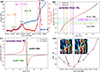 |
Fig. 3. Panel (a): Kinematics of the eruptive structures. Blue and red dots and lines represent the apex height and the derived velocity, respectively. Panel (b): Distribution of the decay index computed from the By component (poloidal field). The cyan-shaded regions indicate the typical threshold for TI (n = 0.8–1.5). The green and red lines show the results derived from the potential field at 04:32 and 05:00 UT, respectively. The orange and pink lines mark the critical height and corresponding decay index at the onset (04:46 UT) and peak (04:56 UT) of the second acceleration phase. Panel (c): Decay-index distribution computed from the Bx component (toroidal field), with the vertical dashed green and black lines indicating the heights where the decay index equals zero and reaches its minimum, respectively. Panel (d): Evolution of the maximum J/B along the horizontal line in the inset J/B images. The vertical dashed red line indicates the time when the maximum J/B begins to increase. |
At the time of the first acceleration, the twisted flux rope had not yet fully formed. Nevertheless, magnetic reconnection within the fan–spine structure above the sheared arcade could already have occurred, initiating the initial rise of the eruptive structures and facilitating the subsequent formation of the flux rope around 04:46 UT. Additionally, the quasi-separatrix layers (QSLs; Priest & Démoulin 1995; Demoulin et al. 1996) associated with the fan–spine topology are very similar to the morphology of the C8.4 flare that peaked at 04:20 UT (Fig. 1e). Additional details on the evolution of the QSLs and the photospheric twist distribution are provided in Fig. B.1. These findings suggest that the first acceleration phase is associated with the C8.4 confined flare driven by fan–spine reconnection.
Afterward, a twisted flux rope forms at approximately 04:46 UT and begins to rise slowly. At this moment, the apex height of the flux rope reaches approximately 11.2 Mm. To investigate the role of TI in its subsequent acceleration, we calculated the decay index at 04:32 UT and 05:00 UT to minimize the influence of the bottom-driven boundaries on the decay-index profile. Figure 3b shows the poloidal-field decay index (np) computed from the poloidal magnetic field component (Bp). Further details on the computation methods and physical meanings of the decay indices are provided in Appendix D.
It should be noted that the critical threshold of TI is not a fixed value; according to previous theoretical analyses (Démoulin & Aulanier 2010) and MHD simulations (Zuccarello et al. 2015), it can vary between n ≈ 0.8 and 1.5. Thus, TI is expected to occur within this range, with corresponding critical heights of 6.9 Mm for n = 0.8 and 18.7 Mm for n = 1.5 (cyan band in Fig. 3b). At 04:46 UT, coinciding with the onset of the second acceleration phase, the flux-rope apex reaches 11.2 Mm, where the decay index is about 1.07. By 04:56 UT, when the rising velocity peaks, the apex height increases to approximately 20.2 Mm, corresponding to a decay index of 1.51, which is close to the commonly adopted critical value of 1.5 (Aulanier et al. 2010). These results suggest that TI likely contributes to the second acceleration stage of the flux rope, with an effective instability threshold in the range n ≈ 1.07–1.51, during which the TI contributes to the rising velocity.
After the second acceleration phase, the flux rope rises to a plateau from 05:04 UT to 05:36 UT, even though the TI is likely already at work. Such a plateau is absent in previous MHD simulations based on simple bipolar configurations (Aulanier et al. 2010). A key difference between our model and the idealized bipole is the presence of strong toroidal magnetic fields (Fig. D.1a), which may induce a downward force (Myers et al. 2015). In Fig. 3c we present the toroidal-field decay index (nt) computed based on Bx, which is approximately aligned with the flux-rope axis. The results show that toroidal-field decay index (nt) becomes negative at a height of 29.7 Mm and reaches its minimum around 30.5 Mm. This indicates that the toroidal-field-induced tension force becomes increasingly dominant at these heights, naturally explaining why the flux rope remains nearly stationary at heights between 30 and 35 Mm during the period 05:04–05:36 UT. The gradual displacement of the flux rope during this stage may be due to moderate magnetic reconnection (Inoue et al. 2018), photospheric driving flows (Liu et al. 2025), or plasma inertia.
After 05:36 UT, the rising velocity of the flux rope increases again and undergoes significant acceleration around 05:40 UT, when the flux rope apex reaches a height of approximately 38.7 Mm. At this height, the (still negative) toroidal-field decay index, |nt|, has diminished to nearly one-tenth of its minimum, suggesting that the overlying toroidal field no longer strengthens rapidly with height. This in turn implies that the downward tension force exerted by the toroidal fields persists to some extent but does not continue to significantly increase with height. The rising speed peaks at 05:46 UT, reaching a value about 3.5 times larger than that of the second velocity peak. To investigate the reasons for this behavior, we examined the temporal evolution of the maximum J/B below the erupting flux rope (Fig. 3d). First, the maximum J/B decreases due to the passage of the rising flux rope. Then, it increases sharply beginning at 05:40 UT, suggesting the onset of fast magnetic reconnection beneath the flux rope, which drives its impulsive upward motion (Jiang et al. 2021).
4. Summary and conclusion
Based on data-driven MHD simulations, we investigated the initiation of the CME associated with an X1.3 solar flare in NOAA AR 13663. The time lag between the observed flare peak and the velocity peak in the simulation is only one minute, demonstrating that our data-driven model closely reproduces observations. Moreover, the simulation reveals multiple stages in the kinematics of the eruptive structure during CME initiation. These results indicate that our data-driven approach is fundamentally capable of modeling CME onset and can serve as an effective tool for determining the physics behind complex observations.
The simulation results indicate that in a magnetic configuration with strong overlying toroidal fields, the kinematics of CME precursors likely evolve through multiple stages: an initial slow acceleration, a plateau at an approximately stable height, and a subsequent impulsive acceleration (Figs. 3a and E.1). These stages are associated with TI (Kliem & Török 2006; Aulanier et al. 2010), the downward tension force of the overlying toroidal field (Myers et al. 2015; Zhong et al. 2021; Guo et al. 2024a; Zhang et al. 2024), and rapid magnetic reconnection (Jiang et al. 2021), respectively. The presence of the plateau suggests that the strong overlying toroidal field can temporarily suppress the eruption. More importantly, the simulation demonstrates that magnetic reconnection acts as the primary trigger of the solar eruption. The appearance of the plateau further implies that, although TI can occur, it does not necessarily lead to a drastic eruption. This indicates that the external magnetic configuration strongly influences CME initiation. As shown in Kliem et al. (2021), a saddle-like profile of the poloidal-field decay index (np) can lead to a confined flare followed by a successful eruption. In this case, however, np increases monotonically, while the toroidal-field decay index (nt) becomes negative above a certain height, where enhanced toroidal tension leads to the plateau stage. The multiple stages during the CME initiation are also found in Zhou et al. (2006), in which the kink instability and filament drainage contribute to the first acceleration, and the reconnection leads to the eruption. These studies indicate that the impulsive phase is governed by fast magnetic reconnection, whereas the preceding moderate acceleration can arise from a variety of mechanisms.
Additionally, the time difference between the observed flare peak and the velocity peak of the flux rope in our simulations is only about 1 minute, highlighting the close agreement between the model and observations. Overall, the results presented in this Letter demonstrate the strong capability of numerical data-driven modeling in accurately reproducing the onset and early dynamics of CMEs, providing a powerful tool for understanding and predicting solar eruptions.
Data availability
Movie associated with Fig. 2 is available at https://www.aanda.org
Acknowledgments
J.H.G., P.F.C., and Y.G. are supported by the National Key R&D Program of China 2020YFC2201200, 2022YFF0503004, NSFC (12503063, 12333009, 12127901) and the China National Postdoctoral Program for Innovative Talents fellowship under Grant Number BX20240159. SP is funded by the European Union. However, the views and opinions expressed are those of the author(s) only and do not necessarily reflect those of the European Union or ERCEA. Neither the European Union nor the granting authority can be held responsible. His project (Open SESAME) has received funding under the Horizon Europe program (ERC-AdG agreement No 101141362). These results were also obtained in the framework of the projects C16/24/010 C1 project Internal Funds of KU Leuven), G0B5823N and G002523N (WEAVE) (FWO-Vlaanderen), and 4000145223 (SIDC Data Exploitation (SIDEX2), ESA Prodex). The numerical calculations in this paper were performed in the cluster system of the High Performance Computing Center (HPCC) of Nanjing University.
References
- Antiochos, S. K., DeVore, C. R., & Klimchuk, J. A. 1999, ApJ, 510, 485 [Google Scholar]
- Aulanier, G., Török, T., Démoulin, P., & DeLuca, E. E. 2010, ApJ, 708, 314 [Google Scholar]
- Chen, P. F. 2011, Liv. Rev. Sol. Phys., 8, 1 [Google Scholar]
- Chen, P. F., & Shibata, K. 2000, ApJ, 545, 524 [Google Scholar]
- Cheng, X., Zhang, J., Kliem, B., et al. 2020, ApJ, 894, 85 [Google Scholar]
- Cheng, X., Xing, C., Aulanier, G., et al. 2023, ApJ, 954, L47 [NASA ADS] [CrossRef] [Google Scholar]
- Chintzoglou, G., Zhang, J., Cheung, M. C. M., & Kazachenko, M. 2019, ApJ, 871, 67 [NASA ADS] [CrossRef] [Google Scholar]
- Chiu, Y. T., & Hilton, H. H. 1977, ApJ, 212, 873 [NASA ADS] [CrossRef] [Google Scholar]
- Démoulin, P., & Aulanier, G. 2010, ApJ, 718, 1388 [Google Scholar]
- Demoulin, P., Henoux, J. C., Priest, E. R., & Mandrini, C. H. 1996, A&A, 308, 643 [NASA ADS] [Google Scholar]
- Fan, Y. 2018, ApJ, 862, 54 [Google Scholar]
- Gosling, J. T. 1993, J. Geophys. Res., 98, 18937 [NASA ADS] [CrossRef] [Google Scholar]
- Guo, Y., Ding, M. D., Schmieder, B., et al. 2010, ApJ, 725, L38 [Google Scholar]
- Guo, Y., Xia, C., Keppens, R., Ding, M. D., & Chen, P. F. 2019, ApJ, 870, L21 [NASA ADS] [CrossRef] [Google Scholar]
- Guo, J. H., Ni, Y. W., Zhong, Z., et al. 2023a, ApJS, 266, 3 [NASA ADS] [CrossRef] [Google Scholar]
- Guo, J. H., Qiu, Y., Ni, Y. W., et al. 2023b, ApJ, 956, 119 [NASA ADS] [CrossRef] [Google Scholar]
- Guo, J. H., Ni, Y. W., Guo, Y., et al. 2024a, ApJ, 961, 140 [NASA ADS] [CrossRef] [Google Scholar]
- Guo, Y., Guo, J., Ni, Y., et al. 2024b, Rev. Mod. Plasma Phys., 8, 29 [Google Scholar]
- Inoue, S., Kusano, K., Büchner, J., & Skála, J. 2018, Nat. Commun., 9, 174 [NASA ADS] [CrossRef] [Google Scholar]
- Jiang, C. 2024, Sci. China Earth Sci., 67, 3765 [Google Scholar]
- Jiang, C., Feng, X., Liu, R., et al. 2021, Nat. Astron., 5, 1126 [NASA ADS] [CrossRef] [Google Scholar]
- Jiang, C., Feng, X., Guo, Y., & Hu, Q. 2022, Innovation, 3, 100236 [Google Scholar]
- Keppens, R., Popescu Braileanu, B., Zhou, Y., et al. 2023, A&A, 673, A66 [NASA ADS] [CrossRef] [EDP Sciences] [Google Scholar]
- Kliem, B., & Török, T. 2006, Phys. Rev. Lett., 96, 255002 [Google Scholar]
- Kliem, B., Lee, J., Liu, R., et al. 2021, ApJ, 909, 91 [NASA ADS] [CrossRef] [Google Scholar]
- Lekshmi, B., Tripathy, S., Jain, K., & Pevtsov, A. 2025, ApJ, 987, 134 [Google Scholar]
- Lemen, J. R., Title, A. M., Akin, D. J., et al. 2012, Sol. Phys., 275, 17 [Google Scholar]
- Liu, R., Kliem, B., Titov, V. S., et al. 2016, ApJ, 818, 148 [Google Scholar]
- Liu, Q., Jiang, C., Bian, X., et al. 2024, MNRAS, 529, 761 [Google Scholar]
- Liu, Q., Jiang, C., & Liu, Z. 2025, Res. Astron. Astrophys., 25, 051002 [Google Scholar]
- Myers, C. E., Yamada, M., Ji, H., et al. 2015, Nature, 528, 526 [Google Scholar]
- Pesnell, W. D., Thompson, B. J., & Chamberlin, P. C. 2012, Sol. Phys., 275, 3 [Google Scholar]
- Priest, E. R., & Démoulin, P. 1995, J. Geophys. Res., 100, 23443 [NASA ADS] [CrossRef] [Google Scholar]
- Schmieder, B., Aulanier, G., & Vršnak, B. 2015, Sol. Phys., 290, 3457 [NASA ADS] [CrossRef] [Google Scholar]
- Schmieder, B., Guo, J., Aulanier, G., Maharana, A., & Poedts, S. 2025, Sol. Phys., 300, 132 [Google Scholar]
- Schrijver, C. J., Kauristie, K., Aylward, A. D., et al. 2015, Adv. Space Res., 55, 2745 [NASA ADS] [CrossRef] [Google Scholar]
- Schuck, P. W. 2008, ApJ, 683, 1134 [NASA ADS] [CrossRef] [Google Scholar]
- Titov, V. S., Hornig, G., & Démoulin, P. 2002, J. Geophys. Res. (Space Phys.), 107, 1164 [Google Scholar]
- Webb, D. F., & Howard, T. A. 2012, Liv. Rev. Sol. Phys., 9, 3 [Google Scholar]
- Wu, H., Guo, Y., Keppens, R., et al. 2025, ApJ, 992, 81 [Google Scholar]
- Xia, C., Teunissen, J., El Mellah, I., Chané, E., & Keppens, R. 2018, ApJS, 234, 30 [Google Scholar]
- Xing, C., Li, H. C., Jiang, B., Cheng, X., & Ding, M. D. 2018, ApJ, 857, L14 [Google Scholar]
- Xing, C., Aulanier, G., Cheng, X., Xia, C., & Ding, M. 2024a, ApJ, 966, 70 [Google Scholar]
- Xing, Y., Duan, A., & Jiang, C. 2024b, MNRAS, 534, 107 [Google Scholar]
- Zhang, J., & Dere, K. P. 2006, ApJ, 649, 1100 [NASA ADS] [CrossRef] [Google Scholar]
- Zhang, J., Dere, K. P., Howard, R. A., Kundu, M. R., & White, S. M. 2001, ApJ, 559, 452 [Google Scholar]
- Zhang, X. M., Guo, J. H., Guo, Y., Ding, M. D., & Keppens, R. 2024, ApJ, 961, 145 [NASA ADS] [CrossRef] [Google Scholar]
- Zhong, Z., Guo, Y., & Ding, M. D. 2021, Nat. Commun., 12, 2734 [NASA ADS] [CrossRef] [Google Scholar]
- Zhong, Z., Guo, Y., Wiegelmann, T., Ding, M. D., & Chen, Y. 2023, ApJ, 947, L2 [Google Scholar]
- Zhou, G. P., Wang, J. X., Zhang, J., et al. 2006, ApJ, 651, 1238 [NASA ADS] [CrossRef] [Google Scholar]
- Zuccarello, F. P., Aulanier, G., & Gilchrist, S. A. 2015, ApJ, 814, 126 [Google Scholar]
Appendix A: Numerical setup of data-driven MHD modeling
To study the initiation process of the CME, we adopt our data-driven MHD model to simulate the evolution of this AR from 04:12 UT to 07:00 UT. The governing equations are as follows:
 (A.1)
(A.1)
 (A.2)
(A.2)
 (A.3)
(A.3)
where B, v, and ρ denote magnetic field, velocity and density, respectively. The initial condition for magnetic fields is provided by the potential-field model with Green’s function (Chiu & Hilton 1977) at 04:12 UT. The density is provided by the hydrostatic solution of a stratified atmosphere from the chromosphere to the corona (Guo et al. 2023a,b, 2024a). Regarding the driven boundary, we adopt the SHARP vector magnetic fields and the derived velocities with the differential affine velocity estimator for vector magnetograms (DAVE4VM; Schuck 2008) method, implementing the v&B-driven boundary (Guo et al. 2024b). They are provided in the cell centre of the inner ghost cell near the physical computational domain, and those in the outer ghost cells are obtained via equal-gradient extrapolation. In particular, to keep the simulation environment closer to observations, we directly use the observational magnetograms and derived velocities without pre-processing, with maximum magnetic fields exceeding 2000 G and driven velocities below 1 km s−1. This approach ensures that the simulation results are directly comparable to real observations, capturing the physical evolution of the eruptive structure with high fidelity. As a result, the evolution of coronal magnetic fields is fully governed by photospheric flows in observations, and the formation and eruption of the flux rope are self-consistent.
The partial differential equations are numerically solved using the message passing interface adaptive mesh refinement versatile advection code (MPI-AMRVAC1; Xia et al. 2018; Keppens et al. 2023). The computational domain is [xmin,xmax] × [ymin,ymax] × [zmin,zmax] = [−172.3,172.3] × [−172.3,172.3] × [1, 345.7] Mm3, with an effective mesh grid of 480 × 480 × 480, adopting a four-level adaptive mesh refinement. In particular, as in Jiang et al. (2021) and Wu et al. (2025), to refine the current sheet in the simulation, an additional adaptive mesh refinement criterion is imposed, J△/B > 0.2, where J is the current density and △ is the spatial grid size.
Appendix B: Distributions of QSLs and twist, and comparison with observations
To compare the simulation results with observations, we compute the distributions of QSLs and the twist number on the bottom plane using the open-source code implemented by Liu et al. (2016), as shown in Fig. B.1. It is found that QSLs closely resemble the morphology of flare ribbons, indicating that the magnetic topology in the simulation results is comparable to that observed. Additionally, it is observed that the accumulation of twist during the CME buildup and the eastern slip of the east footpoint are denoted by high-twist-number regions.
Moreover, although the onset times of the three flare peaks in the observations and the corresponding velocity peaks in the simulations are not perfectly aligned, we still infer that they are physically related. For the first confined flare, the flux rope has not yet formed; the flare ribbons arise from fan–spine magnetic reconnection. The second confined flare is associated with the flux rope rising due to TI, thereby enhancing reconnection above the null point. The third flare is more complex, showing multiple ribbons produced by rapid magnetic reconnection that ultimately trigger the eruption.
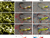 |
Fig. B.1. Comparison of flare ribbons in 1600 Å and the distributions of QSLs and twist on the bottom plane of the simulation. The red contours in the middle column denote the regions with lg Q > 2. The blue/red regions in the right column denote negative/positive twists, respectively. The yellow lines represent the traced eruptive magnetic structures. |
Appendix C: Typical magnetic topology
Here, we present the characteristic magnetic topology during the CME initiation. Figure C.1a shows the sheared arcades and the overlying fan–spine structure at 04:22 UT, where the fan–spine reconnection triggers the C8.4 confined flare. Figure C.1b displays the pre-eruptive twisted flux rope at 04:46 UT. The flux rope contains an inverse magnetic-field component and remains anchored to the photosphere, where the second acceleration phase begins. Figure C.1c illustrates the erupting flux rope together with the current sheet beneath it, in which the purple and green lines represent two groups of sheared arcades prior to the eruption, while the pink lines denote the newly formed field lines after magnetic reconnection. The magnetic reconnection drives the eruption into the impulsive phase. First, as discussed in Jiang et al. (2021) and Jiang (2024), the slingshot effect of the newly reconnected field lines (pink field lines) can efficiently accelerate the eruption. Second, the downward Lorentz force is weak at this height: the poloidal-field decay index np exceeds 1.5, indicating that the strapping field decreases sufficiently rapidly with height to constrain the eruption; and the toroidal-field decay index nt increases from ∼ − 20 to nearly 0, implying that the toroidal-field-induced downward tension force no longer strengthens significantly with height. Consequently, once magnetic reconnection sets in, the eruption can be triggered and accelerated more effectively under reduced constrains. In particular, the purple field lines connect to the eastward negative-polarity sunspot, suggesting that the eastward slipping motion of the eastern flux-rope footpoint could be related to the impulsive magnetic reconnection. Figure C.1d shows the twisted eruptive flux rope at 06:48 UT, revealing that its western leg above the compact polarity inversion line is more highly twisted than the eastern leg rooted in diffused magnetic polarities. In addition, rotational velocity patterns are absent in the velocity-field distribution at the flux-rope footpoints, indicating that the twist does not result from rigid twisting motions in the photosphere. This implies that the enhanced twist is primarily generated through magnetic reconnection during the eruption.
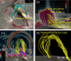 |
Fig. C.1. Typical magnetic topologies involved in CME initiation. Panel (a): Fan–spine structure and sheared arcades at 04:22 UT. Panel (b): Pre-eruptive flux rope at 04:46 UT. Panel (c): Current sheet at 05:46 UT. Panel (d): Twisted eruptive flux rope at 06:48 UT. |
Appendix D: Decay index derived from different magnetic field components
To quantify the influence of external magnetic fields on the triggering and evolution of the solar eruption, we calculate the decay index using the poloidal (Bp), toroidal (Bt), and total horizontal magnetic fields (Bh). The decay index is defined as
 (D.1)
(D.1)
where i = p, t, h corresponds to the poloidal, toroidal, and total horizontal components, respectively. The resulting quantities are referred to as the poloidal-field decay index (np), toroidal-field decay index (nt), and total horizontal-field decay index (nh). Because the pre-eruption flux rope is oriented approximately along the x direction, By and Bx are used as reasonable proxies for the poloidal and toroidal components in the flux-rope coordinate system.
Figure D.1 shows the profiles of np, nt, and nh. These profiles exhibit distinctly different shapes: np shows a monotonically increasing trend, nt displays a dipolar shape (two opposite-sign peaks), and nh presents a unimodal (single-peak) shape. Two features are noteworthy. First, the critical height at which the decay index reaches the threshold value of 1.5 differs among the three profiles, while the second acceleration phase in the simulation occurs when np ∼ 1.5. This highlights the importance of using the poloidal field to compute the decay index relevant to TI, rather than nt and nh. Second, the height of the dip in nt nearly coincides with that of the maximum in nh, which likely corresponds to the height of the plateau stage during the eruption. As a result, based on this data-driven MHD simulation, we suggest that the poloidal-field decay index (np) governs the onset of the solar eruption through the TI (the slow-acceleration phase), whereas the toroidal-field decay index (nt) controls the subsequent evolution (the plateau stage).
This indicates that the initial external magnetic configuration has a significant impact on CME initiation. For instance, as shown by Guo et al. (2010) and Kliem et al. (2021), a saddle-like profile (a rise–fall–rise pattern) of the poloidal-field decay index np can lead first to a confined flare and then to a subsequent eruptive CME. The initial confinement occurs because the poloidal-field–induced strapping force dominates within the torus-unstable regime at the np minimum. In contrast, in the present event, np exhibits a monotonically increasing trend, whereas the toroidal-field decay index nt displays a dipolar profile. The region of negative nt corresponds to a locally strengthening toroidal field, which enhances the toroidal-field–induced tension force, thereby leading to the plateau phase in the CME initiation.
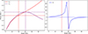 |
Fig. D.1. Profiles of the poloidal-field decay index (np; red), toroidal-field decay index (nt; blue), and total horizontal-field decay index (nh; purple), derived from the corresponding poloidal (Bp), toroidal (Bt), and total horizontal (Bh) magnetic fields. The vertical red and purple lines indicate the heights of np = 1.5 and the maximum nh = 1.84, respectively. |
Appendix E: Multi-stage kinematics of CME precursors in magnetic configurations with strong overlying toroidal fields
Figure E.1 shows the magnetic configuration and the corresponding time–distance diagram of the CME precursors (for example, filament and hot channels) extracted from our data-driven simulation after flux-rope formation. The simulation results indicate that in the magnetic configuration with strong overlying toroidal magnetic fields, the kinematics of CME precursors likely proceed through multiple stages: an initial slow acceleration, a plateau at a nearly stable height, and a subsequent impulsive acceleration (Fig. D.1b).
Based on the analysis in this study and previous works, we propose that the initial slow acceleration corresponds to the slow-rise phase observed in bipole configurations, which can be explained by the direct responses to the current-sheet formation (Xing et al. 2024b; Liu et al. 2025), hyperbolic flux tube reconnection (Cheng et al. 2023; Xing et al. 2024a), and TI (Xing et al. 2024a). In our simulations, the complexity of the photospheric flows makes it difficult to isolate the contribution of each effect individually. We speculate that these effects likely work in combination. Hereafter, in contrast to bipole configurations, where TI-induced acceleration can directly trigger eruptions (Aulanier et al. 2010), or facilitate current-sheet formation beneath the flux rope and thereby initiate the impulsive phase (Xing et al. 2024a). In our case, the presence of strong overlying toroidal fields generates a downward tension force that suppresses further rising (Myers et al. 2015; Guo et al. 2024a), resulting in a plateau stage. The subsequent impulsive acceleration arises from fast magnetic reconnection beneath the flux rope (Jiang et al. 2021), indicating that fast reconnection is the dominant trigger and driver of the eruption. Consistent with the conclusion of Liu et al. (2024), the TI may not necessarily trigger an eruption even in the presence of a pre-existing flux rope. This simulation demonstrates that strong overlying toroidal fields can extend the duration of the buildup phase before the impulsive eruption, thereby improving the prediction of the onset time in real events.
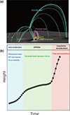 |
Fig. E.1. Magnetic configuration (a) and the corresponding kinematics of the CME precursors (b) during the initiation process. In panel (a), the yellow, pink, and cyan lines represent the CME precursor (flux rope), the overlying poloidal fields, and the toroidal fields associated with the fan–spine structure, respectively. In panel (b), the blue, yellow, and red bands indicate the three stages of the CME precursors. The black line with black dots shows the time–distance diagram of the CME precursors. |
All Figures
|
Fig. 1. Panel (a): Soft X-ray light curves (red: 1–8 Å; blue: 0.5–4 Å) from 04:00 to 08:00 UT on 2024 May 5. The vertical green, sky-blue, and dark blue lines mark the confined C8.4 and C5.5 flares and the eruptive X1.3 flare, respectively. Panels (b)–(d): Composite SDO/AIA 304 Å (red) and 131 Å (blue) images at the peak times of the three flares. Panels (e) and (f): 1600 Å flare-ribbon morphology of the first confined flare and the third eruptive flare, respectively. Panel (g): 3D magnetic field configuration from the data-driven MHD model at 05:00 UT. The green, pink, and cyan lines represent the flux rope, the fan–spine structure, and the surrounding coronal loops, respectively. |
| In the text | |
|
Fig. 2. Evolution of the 3D magnetic field lines in the simulation. The left and right panels show the top and side views, respectively. The field lines are color-coded by magnetic field strength. The side-plane slice displays the electric current density (J), and the gray contours highlight regions of enhanced current. An associated movie is available online. |
| In the text | |
|
Fig. 3. Panel (a): Kinematics of the eruptive structures. Blue and red dots and lines represent the apex height and the derived velocity, respectively. Panel (b): Distribution of the decay index computed from the By component (poloidal field). The cyan-shaded regions indicate the typical threshold for TI (n = 0.8–1.5). The green and red lines show the results derived from the potential field at 04:32 and 05:00 UT, respectively. The orange and pink lines mark the critical height and corresponding decay index at the onset (04:46 UT) and peak (04:56 UT) of the second acceleration phase. Panel (c): Decay-index distribution computed from the Bx component (toroidal field), with the vertical dashed green and black lines indicating the heights where the decay index equals zero and reaches its minimum, respectively. Panel (d): Evolution of the maximum J/B along the horizontal line in the inset J/B images. The vertical dashed red line indicates the time when the maximum J/B begins to increase. |
| In the text | |
|
Fig. B.1. Comparison of flare ribbons in 1600 Å and the distributions of QSLs and twist on the bottom plane of the simulation. The red contours in the middle column denote the regions with lg Q > 2. The blue/red regions in the right column denote negative/positive twists, respectively. The yellow lines represent the traced eruptive magnetic structures. |
| In the text | |
|
Fig. C.1. Typical magnetic topologies involved in CME initiation. Panel (a): Fan–spine structure and sheared arcades at 04:22 UT. Panel (b): Pre-eruptive flux rope at 04:46 UT. Panel (c): Current sheet at 05:46 UT. Panel (d): Twisted eruptive flux rope at 06:48 UT. |
| In the text | |
|
Fig. D.1. Profiles of the poloidal-field decay index (np; red), toroidal-field decay index (nt; blue), and total horizontal-field decay index (nh; purple), derived from the corresponding poloidal (Bp), toroidal (Bt), and total horizontal (Bh) magnetic fields. The vertical red and purple lines indicate the heights of np = 1.5 and the maximum nh = 1.84, respectively. |
| In the text | |
|
Fig. E.1. Magnetic configuration (a) and the corresponding kinematics of the CME precursors (b) during the initiation process. In panel (a), the yellow, pink, and cyan lines represent the CME precursor (flux rope), the overlying poloidal fields, and the toroidal fields associated with the fan–spine structure, respectively. In panel (b), the blue, yellow, and red bands indicate the three stages of the CME precursors. The black line with black dots shows the time–distance diagram of the CME precursors. |
| In the text | |
Current usage metrics show cumulative count of Article Views (full-text article views including HTML views, PDF and ePub downloads, according to the available data) and Abstracts Views on Vision4Press platform.
Data correspond to usage on the plateform after 2015. The current usage metrics is available 48-96 hours after online publication and is updated daily on week days.
Initial download of the metrics may take a while.