| Issue |
A&A
Volume 707, March 2026
|
|
|---|---|---|
| Article Number | A386 | |
| Number of page(s) | 12 | |
| Section | Planets, planetary systems, and small bodies | |
| DOI | https://doi.org/10.1051/0004-6361/202558517 | |
| Published online | 23 March 2026 | |
Solar wind observations at comet 67P around perihelion
Initial transition to a fluid-like flow
1
Swedish Institute of Space Physics,
Box 812,
981 28
Kiruna,
Sweden
2
Umeå University,
Umeå,
Sweden
3
Northumbria University,
Newcastle,
UK
4
Institute of Physics, University of Graz,
Graz,
Austria
★ Corresponding author: This email address is being protected from spambots. You need JavaScript enabled to view it.
Received:
11
December
2025
Accepted:
30
January
2026
Abstract
Context. Rosetta followed comet 67P at heliocentric distances from 1.25 to 3.6 au. Close to perihelion, Rosetta was located in the solar wind ion cavity, with only sporadic observations of solar wind ions. Just outside the solar wind ion cavity, the solar wind ion-flow direction was mainly sunward.
Aims. We aim to study the evolution of solar wind interaction with a comet as its scale size increases from sub-ion gyroradius to above the proton gyroradius. The former was observed at 67P during most of the Rosetta mission. The latter was observed during sporadic solar wind encounters around perihelion.
Methods. We analysed particle data from the mass-resolving ion spectrometer ICA, searching for the weak and sporadic occurrences of solar wind ions close to perihelion. All Rosetta plasma data were used to understand the plasma parameter regime of the observed interaction.
Results. At comet 67P, we observe the transition from solar wind interaction during the first partial gyration of the solar wind ions in the slowed-down plasma around the comet to multiple gyrations in an interaction region larger than the proton gyroradius. During the multiple-gyration stage, the protons show a consistent pattern of motion ordered by the direction of the solar wind electric field. In the hemisphere where the electric field points away from the nucleus, the protons move sunward. They move anti-sunward in the opposite hemisphere. This can be explained by simple trochoid trajectories and a strong density gradient. Under the same conditions, the water ions also show a consistent flow pattern relative to the electric field determined by the point in their gyration at which they pass closest to the nucleus. Protons are slowed down and heated, which is consistent with a shock upstream. The plasma beta is close to one, and the magnetosonic Mach number was typically less than unity.
Key words: solar wind / comets: general / comets: individual: 67P
© The Authors 2026
 Open Access article, published by EDP Sciences, under the terms of the Creative Commons Attribution License (https://creativecommons.org/licenses/by/4.0), which permits unrestricted use, distribution, and reproduction in any medium, provided the original work is properly cited.
This article is published in open access under the Subscribe to Open model. This email address is being protected from spambots. You need JavaScript enabled to view it. to support open access publication.
1 Introduction
Comets are small Solar System bodies characterised by a high content of volatiles and eccentric orbits. When approaching the Sun, the nucleus is heated and releases an increasing amount of volatiles, frequently H2O, CO2, and CO, but also many other compounds (Bockelée-Morvan & Biver 2017). The neutral gas is not bound by the weak gravity of the nucleus, and it moves away at a typical speed of about 0.5–1 km/s relative to the nucleus (Gulkis et al. 2015). The outgassing rate or ‘activity’ of a comet is given in molecules per second released to the surrounding space. Typical values at 1 au from the Sun are about 1030 s−1 for a high-activity comet such as Halley; and 1028 s−1 for medium-activity comets such as Giacobini-Zinner, Grigg-Skjellerup, Borrely, and Churyumov-Gerasimenko around perihelion (Cravens & Gombosi 2004; Hansen et al. 2016). Comet 67P/Churyumov-Gerasimenko (hereafter comet 67P) was followed by the Rosetta mission covering distances out to 3.8 au and an activity down to as low as 1025 s−1 (Hansen et al. 2016).
The neutral gas of the comet is ionised by solar extreme ultraviolet radiation (EUV), electron impact, and charge exchange ionisation, adding charge and mass to the solar wind flow. This addition of mass to a flowing plasma is called mass loading (Szegö et al. 2000). The diffuse addition of mass to the solar wind stream has significant consequences for how the solar wind interacts with the comet obstacle as first realised by Biermann et al. (1967). The newborn ions are picked up by the solar wind flow on the timescale of one cometary ion gyroperiod. Models predict that only a small fraction of cometary ions added to the solar wind flow will result in a weak shock forming. Thus, a shock will form at large distances upstream of the nucleus of medium-to-high-activity comets (Biermann et al. 1967; Ogino et al. 1988; Edberg et al. 2024). The predicted distances for a comet at about 1 au from the Sun correspond well to the distances observed by spacecraft: ~1 million km for Halley, ~100 000 km for Giacobini-Zinner and Borrelly (Cravens & Gombosi 2004), and ~20 000 km for Grigg-Skjellerup (Johnstone et al. 1993).
The shocks that form due to mass loading are weak and broad, with fast flows also on the downstream side. From Halley, speed changes from about 300 km/s to 250 km/s were reported at the bow shock. The proton speed gradually decreased to about 100 km/s in the region where cometary ions dominated the flow (Balsiger et al. 1986; Coates et al. 1990; Formisano et al. 1990). At the lower activity comet Grigg-Skjellerup, a gradual slowing down of the solar wind from about 400 km/s upstream to 100 km/s at closest approach was also observed (Johnstone et al. 1993). The magnetic field data showed a distinct shock feature on the outbound pass, but only a change in wave characteristics on the inbound pass (Neubauer et al. 1993). The temperature of the solar wind ions also showed relatively weak features with proton temperatures in the cometosheath (downstream of the shock) in the 20 eV to 50 eV range (Neugebauer et al. 1987; Formisano et al. 1990). MHD models can reproduce the Giotto observations made at Halley quite well (Rubin et al. 2014).
The Rosetta mission followed 67P for 2 years (Taylor et al. 2017; Glassmeier et al. 2007a). For much of the mission, the activity of the comet was very low, and the scale size of the comet plasma environment was much smaller than a comet pick-up ion gyroradius. This strongly affected the solar wind interaction (Nilsson et al. 2017, 2018; Nilsson et al. 2020). As activity increased around perihelion, there was likely a bow shock upstream of Rosetta; the comet activity was close to that of Grigg-Skjellerup during the Giotto encounter (~1028 s−1). Rosetta was too close to the nucleus to directly observe any bow shock that formed. During most of the time around perihelion, Rosetta did not observe any solar wind ions downstream of the shock. Rosetta was located within a solar wind ion cavity (Behar et al. 2017; Nilsson et al. 2017). Some solar wind ions were seen at the end of a dayside excursion the Rosetta spacecraft made near perihelion (Edberg et al. 2016). During this excursion, a coronal mass ejection (CME) hit the comet environment while Rosetta was at a relatively large distance from the nucleus: 600–1000 km. Features in pick-up ion energy spectra observed inside the solar wind ion cavity during this time can be interpreted as indirect observations of a cometary bow shock (Nilsson et al. 2018; Alho et al. 2019; Alho et al. 2021).
Though no fully developed bow shock was seen, a developing shock structure, the ‘infant’ shock was detected on two occasions (Gunell et al. 2018); it was identified by a simultaneous broadening of proton and electron energy spectra and an enhanced magnitude of the magnetic field. Warm protons indicative of a possible upstream shock were identified on many occasions (Goetz et al. 2021).
For comet–solar wind interaction on a scale much smaller than a comet’s ion gyroradius, newborn cometary ions are consistently moving approximately along the solar wind electric field direction throughout the interaction region. The solar wind is deflected in the opposite direction, conserving momentum. The latter can be seen as a gyration of the solar wind ions in the slowed-down plasma consisting of both solar wind and cometary ions (Behar et al. 2018). Just before and after the time period when Rosetta was in the solar wind ion cavity, the observed protons were typically moving sunward (Behar et al. 2017; Nilsson et al. 2017). This indicates that they were on the second quarter of their first gyration. Partial rings of solar wind ions were observed on a few occasions (Moeslinger et al. 2023), reflecting electric and magnetic field structures on the proton gyroradius scale (Moeslinger et al. 2024). At times, a randomisation of observed proton flow directions relative to the upstream solar wind electric field direction was observed (Williamson et al. 2022). This indicated that solar wind protons started to experience more than one gyration before being observed. This can be interpreted as the deflected solar wind proton flow having turned into a cometosheath flow, which is characterised by a thermalised flow of slowed-down solar wind ions.
In the time period of the solar wind ion cavity sporadic occurrences of low-flux solar wind ions have been seen in the Rosetta ion data (Behar 2018). These are likely to represent a further evolution of the sunward flows (Behar et al. 2017) and later observed multiple gyrations of the protons (Williamson et al. 2022). The purpose of this study is to identify proton observations as close to perihelion as possible and interpret them in terms of how the initial deflection of the solar wind gradually turns into a more fluid-like flow around the comet obstacle.
2 Method
2.1 Instrument description
We mainly used data from the Ion Composition Analyser (ICA) (Nilsson et al. 2007) and the magnetometer (MAG) (Glassmeier et al. 2007b), part of the Rosetta Plasma Consortium (RPC) (Carr et al. 2007). The Ion Composition Analyser is a mass-resolving ion spectrometer with an energy range of a few electronvolts to 40 keV distributed over 96 energy channels We refer the reader to Nilsson et al. (2015, 2017), Stenberg Wieser et al. (2017), and Bergman et al. (2020) for an updated description of the lower limit of the energy range. ICA has a near-2π sr field of view achieved through electrostatic entrance deflection out of the 360° field of view in the detector plane. The field of view is divided into 16 azimuth sectors covering 360° and 16 elevations covering approximately ±45°. Elevations are scanned through in sequence, referred to here as an ‘ICA scan’, which takes 192 s. After the elevation deflection entrance system, ions pass through an electrostatic analyser energy filter, a post-acceleration section, followed by a magnetic assembly. At each elevation step, all 96 energy levels are scanned, which takes 12 s. The magnetic field provides mass resolution, bending the ion trajectories to hit the detector at different radii depending on mass and energy. Ions are detected by anodes at different radii of the detector. There are 32 mass anodes, which we denote ‘mass channels’. ICA has a mass resolution allowing for the resolution of 1, 2, 4, 8, 16, and 32 amu ion masses per elementary charge (amu/e).
In this study, we used the RPCICA L2 and RPCICA L4 PHYS-MASS datasets in the Planetary Science Archive (PSA) of the European Space Agency. The data are further described in Nilsson (2021). The PHYS-MASS data-processing includes a manual selection of energy and mass channel ranges for each species from daily summed energy to mass channel spectra (Behar et al. 2016). This allows for very-high-quality data as long as the signal is strong enough to be seen in the daily summed data. This was not always the case (Behar 2018). Weak and sporadic occurrences of a signal may be lost in the noise when summed over a day, in particular around perihelion, when noise levels were frequently elevated. Therefore, we identified possible weak signals of protons from the L2 data. Possible events were then manually inspected; see Sect. 2.3 for more details.
The magnetometer on Rosetta had a maximum sampling rate of 20 Hz; sometimes only lower data rates were available. In this study, we averaged the magnetic field data over one ICA scan of 192 s. The accuracy of the magnetic field is about 3 nT per component (Goetz et al. 2016, 2017). We used MAG data v9 from PSA.
The ion and electron sensor (IES) (Burch et al. 2007) provided distribution functions of electrons and ions. The ion measurements do not have mass resolution and cannot be used for this study, in which cometary ions and protons typically have similar energies and flow directions. The IES data used is v2.0 from PSA.
We used the Langmuir probe (LAP) (Eriksson et al. 2007) and the mutual impedance probe MIP (Trotignon et al. 2007) to obtain the total plasma density. We employed the L5 NED dataset from PSA, which uses the LAP spacecraft potential proxy for density, calibrated with MIP data when available.
2.2 Temperature and speed estimates
Moments of the ion data were calculated by integration over the ICA field of view following standard procedures (Fränz et al. 2006; Nilsson et al. 2020). A one-dimensional temperature was estimated by summing over all directions and then integrating for a one-dimensional drift and temperature estimate. This is similar to what was done in Williamson et al. (2024), though the authors fitted drifting Maxwell-Boltzmann distributions to measured cometary one-dimensional distributions. The measurements were obtained as a differential flux as function of energy and two angles describing direction, which were integrated into the following one-dimensional flux:
![Mathematical equation: $\[j_{1 D}(E)=\iint ~\cos~ \theta ~j(E, \theta, \phi) d \theta d \phi,\]$](/articles/aa/full_html/2026/03/aa58517-25/aa58517-25-eq1.png) (1)
(1)
where j is differential flux (s−1 m−2 sr−1 eV−1), ϕ and θ are the azimuth and elevation of the instrument view direction, and E is the energy of the particles. The density of the particles (zeroth-order moment) is obtained as
![Mathematical equation: $\[N=\int j_{1 D}(E) \sqrt{\frac{m}{2 E}} d E.\]$](/articles/aa/full_html/2026/03/aa58517-25/aa58517-25-eq2.png) (2)
(2)
The one-dimensional mean speed of the particles was calculated as
![Mathematical equation: $\[v_{1 D}=\frac{1}{N} \int j_{1 D}(E) d E,\]$](/articles/aa/full_html/2026/03/aa58517-25/aa58517-25-eq3.png) (3)
(3)
where N is the density of the particles. The one-dimensional temperature was then calculated through
![Mathematical equation: $\[T_{1 D}=\frac{1}{N} \int \frac{1}{2} m\left(\sqrt{\frac{2 E}{m}}-v_{1 D}\right)^2 j_{1 D}(E) \sqrt{\frac{m}{2 E}} d E.\]$](/articles/aa/full_html/2026/03/aa58517-25/aa58517-25-eq4.png) (4)
(4)
The one-dimensional speed is the average speed of particles; the magnitude of the particle’s bulk velocity may be much lower. To show how these temperature and drift-speed estimates relate to the measured energy spectra, in Fig. 1 we show an example of a measured distribution function taken on 28 May 2015 at 05:36:31 (filled lines). This is compared to a Maxwellian distribution with the one-dimensional drift and temperature as obtained from the integration of the measurements (dotted lines). The lower part of the measured proton energy spectrum is cut off by the sensitivity of the instrument; this is indicated by the one-count (black) line showing the lowest phase-space density the instrument can measure. Both upper and lower energy borders of the measured distribution frequently show sharper declines than the Maxwellian distributions. These lower count parts of the distributions contribute much less to the integrated temperature than the centre of the distribution. These sharper cut-offs could be due to a velocity-filter effect. Investigating that is outside the scope of this paper.
2.3 Data selection
We developed an algorithm to identify weak and/or sporadic signals of protons and alpha particles that may have been lost in the noise in the standard selection procedure. High-time-resolution two-dimensional data (Stenberg Wieser et al. 2017) were excluded. The period investigated was from 22 April 2015 to 7 January 2016. The chosen dates correspond to the time period of the solar wind ion cavity (Behar et al. 2017) and about one month before and after it, when solar wind presence was less continuous. The dates were chosen from manual inspection of daily energy spectra plots to judge the presence of a solar wind signal in the standard (PHYS-MASS) dataset. The resulting dataset consists of a total of 79479 ICA scans of 192 s. The mass channels corresponding to solar wind ions (1–4 amu/e) and energy channels above 80 eV were then summed over all sectors and elevations providing one value per full ICA scan of 192 s. Similarly, mass channels 26 and 27 were summed, as these correspond to the main signal of protons at solar wind energies and below (Nilsson et al. 2007; Nilsson et al. 2015). If the former signal showed more than 20 counts, or the latter more than five counts, a possible signal was registered. For all possible detections, the energy-mass matrix was plotted and the energy and mass channels of H+, He2+, and He+ were manually selected. If no selection was made, the data point (the scan) was discarded. An example from the selection process is shown in Fig. 2. After this selection, a total of 1149 ICA scans remained. An overview plot was created for each scan. This overview plot contained field-of-view plots of protons and alpha particles, when present, as well as of cometary ions; see Moeslinger et al. (2023) for further details on this type of plot. Solar wind, cometary ion, and electron energy-time spectra and the magnetic field data for one hour before and after the detected signal were also plotted. This showed that the solar wind ion signal was frequently seen from the same direction and at the same energy levels as a strong cometary ion signal. A careful check that the solar wind signal was not contaminated by cross-talk from the cometary ion signal was then performed. Presence of a signal in the solar wind mass channels showed no correlation with the presence of a signal in the mass channels corresponding to water ions for a given energy and direction; see Appendix A. Thus, we could conclude that cross talk was not significant. Finally, moments were calculated for the solar wind signal identified.
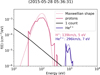 |
Fig. 1 One-dimensional distribution functions for H+ (red) and He2+ (blue). Solid lines show measurements, and dotted lines show Maxwellian distributions with the temperature and drift velocity as calculated from numerical integration of the observations. |
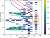 |
Fig. 2 Screenshot from energy-mass channel-selection script. The user draws a box and identifies the ion species for any significant signal. Selected data are shown with a red box for H+, a blue box for He2+, and a green box for He+. Two red lines delineate the expected position of the H+ signal; a blue line shows the border between He2+ and He+. The colour-scale shows the logarithm of the number of counts. The shown signal is summed over all directions. |
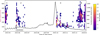 |
Fig. 3 Cometocentric distance of Rosetta (km) as function of time is shown with a black line (right y-axis). The mean speed of the observed solar wind protons (km/s on the right y-axis) is shown with occurrence in time-velocity bins using a colour-scale. The four periods discussed in the text are marked with numbers in the top of the plot. The beginning of the data, from 28 May 2015, is marked with an arrow. |
2.4 Coordinate system
The initial data from PSA uses the body-centred Comet–Solar–Equatorial (CSEq) coordinate system (Acton Jr 1996; Acton et al. 2018). The comet body is at the origin, and x points towards the sun. The z-axis points along the part of the solar north pole axis that is orthogonal to x. The y-axis completes a right-handed system. The spiceypy wrapper was used to access the SPICE toolkit (Annex et al. 2020).
On the data shown in the figures, we used the Comet–Solar–electric field (CSE) coordinate system. Here, x is towards the Sun, and z is rotated so that it is along the component of an estimated solar wind electric field direction in the plane perpendicular to x. Because of the assumptions made, y is along the component of the magnetic field in the plane perpendicular to x, but it also completes a right-handed system. The electric field direction was calculated assuming an E × B drift of the solar wind in the x direction and using the local magnetic field observations (Edberg et al. 2019).
3 Results
The 1149 cases identified through our data-selection process are shown in Fig. 3 with a colour-coded occurrence rate. The indicated data points correspond to 1.4% of all the data points (scans) in this time period. The distance to the nucleus is shown as a black line (right vertical axis). The horizontal axis shows the time in the year-month (UT) format. One can identify four main periods of observations, indicated with numbers one to four in the top of the figure. The first and last periods (numbered 1 and 4) correspond to the same region, just outside the solar wind ion cavity and at a distance of about 100 km from the nucleus. The particle’s mean speed is typically solar wind-like at about 400 km/s. The second period is seen from the end of May to early July at somewhat larger nucleus distances of 200–300 km. Particle speeds are frequently below typical solar wind speeds at about 100–200 km/s. Finally, the return from the dayside excursion at nucleus distances of 200–1100 km forms a third period. For the studied time period, H2O dominated the neutral outgassing (Rubin et al. 2019) and the cometary ions. We assume throughout this text and in the moment calculations that the cometary ions have the mass of H2O. One case on 28 May 2015 stands out in the data from period 2 as it contributes a large number of data points. The day is marked in Fig. 3 with an arrow. The data were obtained at a distance of about 300 km from the nucleus. This is a somewhat larger distance than for most data during this period, except the dayside excursion. Figure 4 shows energy spectrograms from part of 28 May of (a) electrons, (b) cometary ions, and (c) H+. Note the very different colour-scales for each panel. This is followed by (d) the magnetic field components, (e) the H+ velocity moment, (f) the one- and three-dimensional integrated temperature estimates, and (g) the position of the spacecraft in the CSE y–z plane.
The electron data show some features. Examples are intensifications at about 02:30 and 04:30, both correlated with intensification of cometary ion fluxes. The average electron energy spectra during proton events and when no protons are seen show no discernible difference (not shown). The cometary ions show rather broad energy spectra ranging from a few tens of electronvolts up to about 1 keV, with a notable dropout seen at 04:30. The flux dropout coincides with a change of the magnetic field direction to primarily in the negative Bz direction (panel b versus panel d). Judging from field-of-view plots (not shown), this is likely a field-of-view effect, with the main cometary ion population moving outside the instrument’s field of view (Berčič et al. 2018). The appearance and disappearance of the H+ signal appears less related to the magnetic field direction. At about 02:30, there is an intensification of cometary ion fluxes and appearance of H+ fluxes coincident with a flip of the magnetic field direction and a change in spacecraft position from zCSE < 0 to zCSE > 0. There is no obvious preference for an occurrence of solar wind ions for zCSE > 0 otherwise during the shown time period. The H+ velocity is mostly anti-sunward (negative vx), scattering around zero in the other components. The flow relative to the position of the spacecraft in the CSE reference frame is further discussed in the next section. The proton energy is much lower than in the undisturbed solar wind, centring on about 100 eV. The width of the proton energy spectra (panel c) is time varying, as reflected in the integrated temperature estimates (panel f). Solar wind temperatures estimated from dedicated solar wind instruments are typically in the range of 5–15 eV at 1 au (Wilson III et al. 2021). The integrated temperatures from ICA are larger than this, averaging 80 eV over the plotted interval. The one-dimensional temperature averages 10 eV. In Sect. 3.2, we discuss how the ICA-estimated temperatures reported in this study compare to those obtained over the entire mission.
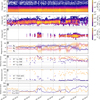 |
Fig. 4 Overview of data from 28 May 2015. In all panels, the x-axis shows the time (UT). Top three panels: differential flux integrated over all observed angles using a colour-scale (cm−2 s−1 eV−1) with particle energy (eV) on the y-axis: electrons (panel a), water ions (panel b), and protons (panel c). Panel d: magnetic field components in the CSEQ coordinate system (nT). Thick lines are averaged over one ICA scan of 192 s. Panel e: proton velocity in the CSE reference frame (km/s). In both cases, dark blue is used for x, red for y, and orange for z. Panel f: integrated temperature estimates for protons. The one-dimensional temperature is shown in dark blue, and the three-dimensional temperature is given in orange. See the text for details on temperature calculations. Panel g: position of Rosetta in the y–z plane, with the distance along the magnetic field direction (CSE y) in dark blue and the distance along the electric field (CSE z) in orange (km). |
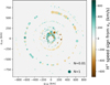 |
Fig. 5 Proton observations in CSE y–z plane (circles). The colour of the circles indicates the mean particle speed with sign from the x component of the velocity moment (km/s). The size of the circle is a linear function of the of the density. The sizes corresponding to 0.01 and 1 cm−3 are shown in the lower right. |
3.1 Spatial distribution of observations
To see if the events observed have a consistent distribution in the CSE reference frame, we plot the data as function of position in the y–z CSE plane. In Figs. 5 and 6, the horizontal axis shows the location along yCSE, and the vertical axis shows the position along zCSE. In Fig. 5, the size of the shown dots is a measure of the H+ density, while the colour gives the mean particle speed of H+ with sign from the vx velocity component. The data from just before and after the solar wind ion cavity are seen at the centre at about 100 km from the nucleus. Sunward flows dominate, as indicated by the blue-green colour. The May–June data are seen at a 200–300 km distance, and anti-sunward flow dominates for zCSE < 0, as shown in brown. At the largest distances from the nucleus, corresponding to data from the dayside excursion, both sunward and anti-sunward flows appear approximately as often as each other. We present the statistics of flow directions and magnitudes in Sect. 3.2.
Figure 6 shows the strength of the magnetic field with sign from the Bx component using a colour-scale. In the CSE reference frame used, the magnetic field in the y–z plane is always along y. Negative Bx values (red) are seen for positive y, and positive Bx values (grey) are seen for negative y positions. This is consistent with draping of the magnetic field. The draping pattern is very clear for these cases, as is common for cases in and around the solar wind ion cavity, but not for low-activity and small-nucleus distances for the whole mission (Goetz et al. 2017). The magnetic field draping during the dayside excursion was extensively studied by Volwerk et al. (2019). For lower activity with a strong deflection of the solar wind, Koenders et al. (2016) showed that draping in the y–z plane dominated close to the nucleus, with field lines stretching towards the negative electric field (z) direction. Such a draping would not show up consistently in our plot.
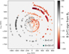 |
Fig. 6 Magnetic field observations in the y–z plane (circles). The colours of the circles show the magnitude of the magnetic field (nT) with sign from the Bx component. The sizes corresponding to 5 and 50 nT are shown in the lower right. |
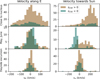 |
Fig. 7 Histograms of proton speed observed close to the nucleus (upper panels) in May and June 2015 (middle panels) and during the dayside excursion (lower panels). Left panels: velocity along the electric field component in the y–z plane. Right panels: sunward velocity (km/s). Brown indicates data for positive zCSE, and blue–green indicates data for negative zCSE. |
3.2 Statistical results
The statistical distribution of proton flow directions is shown using histograms in Fig. 7. The data were divided into three regions: the close-to-the-nucleus data (upper panels), representing the time just before and after the solar wind ion cavity (regions 1 and 4 in Fig. 3); the May–June period data (middle panels); and the dayside-excursion data (lower panels). The flow along the electric field direction (left column) is generally rather symmetrically distributed around zero for both the positive and negative zCSE hemispheres. The flow close to the nucleus is predominantly sunward, while the dayside excursion shows nearly stagnant flows averaging close to zero in the x direction. The May–June data show a clear hemispheric asymmetry with mostly sunward flow for zCSE>0 and anti-sunward flow for zCSE<0. The median values and the percentiles are listed in Table 1.
The close-to-the-nucleus data (periods 1 and 4) show a strong hemispheric asymmetry in the number of events, with many more events for zCSE>0. Figure 8 shows the occurrence of events (blue-green line, lower x-axis) and the total number of samples as function of distance along zCSE (black line, upper x-axis) for periods 1 and 4. The right panel of Fig. 8 features a zoomed-in view of Fig. 5, showing that there are many fewer observations of protons at zCSE<0. At the nucleus distances where we see events, more than approximately 30 km from the nucleus along zCSE, there are slightly more samples for zCSE>0, but a higher occurrence frequency is the main reason for the larger number of events for zCSE>0.
Histograms of the H2O+ flow speed along the electric field and Sun directions are shown in Fig. 9, following the same format as Fig. 7. The speed along the electric field direction of H2O+ is evenly distributed around zero for the region close to the nucleus (median magnitude less than 3 km/s) and the dayside excursion (median magnitude less than 4 km/s) for both electric field hemispheres. The only clear asymmetry concerns the May–June cases, where the flow is typically against the electric field for zCSE above zero and along E for zCSE below zero. The cometary ions have dominating anti-sunward flow for all times and regions, with very few exceptions. An asymmetry is seen in the May–June period with a tail towards higher anti-sunward velocities for zCSE < 0. The median values are listed in Table 1.
Velocity components (km/s) for H+ and H2O+ for three different regions.
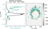 |
Fig. 8 Left: occurrence frequency of solar wind observations (green line, lower x-axis), and total number of observations (black line, upper x-axis). Data are from periods 1 and 4 of Fig. 3, but at the beginning and end of the solar wind ion cavity. Right: zoomed-in view of Fig. 5 with the same zCSE axis as the left panel. The colour shows the speed of H+ with a sign from vx. |
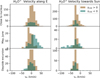 |
Fig. 9 Histograms of H2O+ speed observed close to the nucleus (upper panels) in May and June 2015 (middle panels) and during the dayside excursion (lower panels). Left panels: velocity along the electric field component in the y–z plane. Right panels: sunward velocity (km/s). Brown indicates data for positive zCSE, and blue-green indicates data for negative zCSE. |
3.3 Observed properties of the plasma environment
At this point, we had characterised the plasma environment in terms of ion-flow directions relative to the Sun and the electric field. Next, we proceeded to make estimates of typical plasma parameters for the different observational regions. In Table 2, we tabulate the median plasma density, H+ fraction of density, one-dimensional H+ temperature, magnetic field strength, standard deviation of the magnetic field during one ICA scan, Alfvén speed, magnetosonic speed, plasma flow speed, Alfvén and magnetosonic Mach numbers, plasma beta, and H+ and H2O+ gyro radii. Details on the calculations are given below. The 10th and 90th percentiles are given for all median values. The density (from LAP-MIP) and magnetic field values were first averaged over one ICA scan of 192 s before the medians were calculated.
The low fraction of H+ of the total density (NH+/N) shows that H+ is a minor species for all the investigated times. The plasma speed estimates (vlow and vhigh) of Table 2 were calculated by summing the directional flux of all ion populations observed by ICA and then adding a cold ion flux. The cold flux was assumed to have a density making the total density of all ions equal to the LAP-MIP density estimate (or zero, should the total ICA-derived densities be higher than the LAP-MIP estimate, which happened on a few occasions). The flow direction of the cold component was assumed radially out from the nucleus. The speed was assumed to be 1 km/s (the order of magnitude of neutral gas flow) for vlow or the same as the magnitude of the ICA below 60 eV H2O+ velocity moment for the vhigh of Table 2. Cometary ions below about 60 eV typically from a separate population that is not significantly influenced by the solar wind electric field. See Nilsson et al. (2020) for a discussion on the division of ICA H2O+ moments into two energy ranges. The values of vhigh are similar to the bulk drift speed found by Williamson et al. (2024) by fitting distribution functions to low-energy ion spectra.
As the speeds of H+ and picked-up H2O+ (above 60 eV) shown in Table 1 are much higher than the mean plasma speed (vhigh), they mainly represent a gyration. We can therefore use the particle speed perpendicular to the magnetic field to obtain an estimate of the ion gyroradius. We tried doing this with the velocity moment both as it is and after subtracting the velocity of vhigh as defined above. The latter is the appropriate way if our total plasma velocity estimate is indeed a correctly determined plasma drift velocity. In Table 2, we show the gyroradius calculated from the observed magnetic field and the field-perpendicular component of the velocity moment of H+ and picked-up H2O+ with vhigh subtracted. The subtraction of vhigh changes the value by up to about 10%. Thus, the uncertainty of the ion speed has only a minor impact on the gyroradius determination. It is notable that the H+ gyroradius decreases from close to the nucleus to the May–June period and is at a minimum during the dayside excursion. The H2O+ ions show much less variation, with a factor-of-two lower gyroradius during the dayside excursion compared to the other times. This reflects that H2O+ energy and the magnetic field strength are relatively constant, while the H+ energy goes down closer to perihelion (during the dayside excursion).
The plasma beta was calculated as
![Mathematical equation: $\[\beta=\frac{p_{k i n}+p_T}{p_B},\]$](/articles/aa/full_html/2026/03/aa58517-25/aa58517-25-eq5.png) (5)
(5)
where pT is the thermal pressure of the ions and electrons, and pkin is the kinetic pressure of the minor species. As discussed above, the minor species are moving at speeds well above the mean plasma speed, so the corresponding kinetic pressure is not the true kinetic pressure of a bulk flow. We treated it as a non-gyrotropic component of thermal pressure. The thermal pressure was calculated using integrated moments for the ions detected by ICA and assuming a 10 eV temperature for the electrons, a value found by Galand et al. (2016) to be a good approximation for photoelectrons in the coma that have not undergone energy degradation.
In order to calculate the Alfvén speed, vA, and the magnetosonic speed, vMS, a cometary ion density was calculated as the LAP-MIP density minus the solar wind ion density determined from ICA measurements. On the very few occasions when this number was negative, it was set to zero. The average mass density, ρ, was then determined by assuming the cometary ions were all H2O+. For the magnetosonic speed, we thus have
![Mathematical equation: $\[v_{M S}=\sqrt{v_A^2+\gamma \frac{p_T}{\rho}},\]$](/articles/aa/full_html/2026/03/aa58517-25/aa58517-25-eq6.png) (6)
(6)
where γ is the ratio of specific heats 5/3.
The median of the one-dimensional H+ temperature for the whole mission was 2 eV, compared to 14 eV for this study. For the three-dimensional temperature, the corresponding medians were 78 eV for the entire mission and 89 eV for this study. The higher one-dimensional temperature indicates more broadening of the energy spectra for the data in this study. The smaller difference between the three-dimensional temperatures of this study and the whole mission indicates similar or smaller angular scattering for our dataset as compared to the whole mission. The values in Table 2 show significantly larger one-dimensional temperatures for zCSE> 0 in the May–June case, 19 eV versus 7.0 eV in the zCSE < 0 hemisphere. Otherwise, the differences between regions are small compared to the spread of the data points indicated by the 10th and 90th percentiles.
For the magnetic field, the median standard deviations during one ICA scan were 2.1 nT for the whole mission and 6.4 nT for this study. The median values for the different regions span from 4.8 to 12 nT, all well above the median for the whole mission. The May–June period shows an asymmetry with values for zCSE < 0 being half of those for zCSE > 0.
Plasma parameters for three different regions divided into two hemispheres corresponding to the sign of zCSE.
4 Discussion
One of the most striking results on H+ flow at 67P is the sunward flows of periods 1 and 4 in Fig. 3 observed just before and after the solar wind ion cavity around perihelion (Behar et al. 2017). Our data show that these observations have a spatial asymmetry; the solar wind is observed more frequently for zCSE > 0. The zCSE < 0 region appears shadowed from solar wind ions (Fig. 8). The asymmetry is in agreement with the simplified ion trajectory model of Behar et al. (2018) and a kinetic model for lower activity comets (Deca et al. 2025).
The H+ flow directions seen in the May–June 2015 period have evolved and show a new consistent pattern. For zCSE > 0, the flow was still mainly sunward, while it was mainly anti-sunward for zCSE < 0. This can be understood in terms of when gyrating ions are closest to the nucleus for positive and negative zCSE, respectively. H+ are closest to the nucleus when moving sunward for zCSE > 0, while for zCSE < 0 they are closest when they move anti-sunward, as illustrated in Fig. 10. The solar wind ions observed in May–June 2015 are likely past their first gyration (Williamson et al. 2022), and the consistent flow directions we see are due to a spatial effect of the ion motion at the innermost edge of the solar wind ion flow around the solar wind ion cavity. The innermost region with consistent sunward or anti-sunward motion must then be at most one gyroradius thick. The gyroradius is several 10 km in the May–June case (Table 2), making this a plausible explanation for the consistent observations from May–June. The H+ density was nearly four orders of magnitude lower than the cometary ion density, making a rather clear gyration pattern likely for such a minor species. This also points to a relatively sharp gradient in the solar wind ion density, consistent with a well-defined solar wind ion cavity. The much smaller H+ gyro radius during the dayside excursion would then also explain why we do not see the same consistent pattern there. The May–June data correspond to a heliocentric distance of 1.54 au and a comet activity of 2 · 1027 s−1 (Hansen et al. 2016).
The dayside excursion observations represent the solar wind ion flow observed closest to perihelion. A strong CME pushed the solar wind close enough to the comet to be observed (Edberg et al. 2016). The H+ bulk speed was the lowest observed in our study, with medians of 48 km/s (zCSE>0) and 38 km/s (zCSE<0). The median flow in the x-direction was nearly zero, and the estimated proton gyroradii were the smallest of our observations at 7.7 and 8.4 km. Plasma beta was of about unity, while Mach numbers were typically below one. This could thus represent the most ‘fluid-like’ conditions for the protons we have seen from the Rosetta mission. The protons have time and room to experience multiple gyrations, and the comet magnetosphere environment is at least an order of magnitude larger than a proton gyroradius (tens of kilometres in gyroradius versus hundreds of kilometres in nucleus distance). The H+ density was three orders of magnitude lower than the cometary ion density, so this need not reflect the plasma behaviour in general for these conditions. The H2O+ gyroradius was an order of magnitude larger than the H+ gyroradius, while it was up to an order of magnitude lower than the distance between the spacecraft and the comet, that is, significantly smaller than the comet’s magnetosphere environment. This environment could thus be similar to what was observed at more active comets inside the cometopause. The dayside excursion corresponds to a heliocentric distance of 1.4 au and a comet activity of ~1028 s−1 (Hansen et al. 2016), which is similar to the case of Grigg-Skjellerup at the Giotto encounter. The appearance or disappearance of the solar wind ions thus points to a relatively sharp solar wind ion cavity still present for these conditions at 67P. At Halley, a cometopause where cometary ions started to dominate was reported (Gringauz et al. 1986; Amata et al. 1986; Tátrallyay et al. 1995), and disputed (Reme et al. 1994), where a quite sharp drop in the relative abundance of H+ was observed, but not a sharp drop in its absolute abundance.
There are only a few observations of He2+ in the May–June and dayside excursion events. For May–June, the few observations are consistent with the H+ results. The lack of He2+ here is likely due to low fluxes below the observation threshold. There are also rather frequent observations of only He2+, with no H+ throughout the time period investigated. We leave a more detailed exploration of these events for a future study. He2+ observations are common in the close to nucleus cases of this study. In total, He2+ was observed in 566 out of 1149 data points.
Pick-up ions (H2O+ with energy levels above 60 eV) show a somewhat different flow direction than H+. On their first gyration, H2O+ start out moving along the electric field and thus along +zCSE. From a simplistic trajectory point of view, they are closest to the nucleus in the zCSE > 0 hemisphere when they are past their first quarter of a gyration and move back against the electric field. They are closest to the nucleus in the zCSE < 0 hemisphere when they move along the electric field; see Fig. 10 for an illustration. Both these predictions agree with the data for the May–June period. Thus, the observational results can be understood in terms of simple particle trajectories of pick-up ions. The highest speeds are seen for zCSE < 0, which is consistent with motion along the electric field. In the zCSE > 0 case, the pick-up ions have started to move against the electric field and decelerate.
For all four of our time periods, the energetic pick-up ions dominate the flux and, even more so, the energy flux of ions. Plasma beta is close to unity; the magnetic field pressure is similar to the dynamic pressure of the pick-up ions. This is typical for this time period (Williamson et al. 2020). The Alfvén velocity is low due to the dense plasma and comparatively weak magnetic field. The plasma flow is also slow due to the density being dominated by slow, locally produced plasma, resulting in an Alfvén Mach number around one. The magnetosonic Mach number was typically below one, so the flow is mostly sub-magnetosonic. The solar wind ions reported here are a minor species and not relevant to any local shock formation. Instead, the pick-up H2O+ ions have taken over the role of the solar wind ions, as described for the whole dataset in Nilsson et al. (2020). Both plasma beta close to one and a Mach number close to one indicate a plasma parameter regime where few simplifying assumptions can be made.
All observations are well inside the cometopause if this is defined as where cometary ions start to dominate the density or flux of ions. The observations are also outside the H+ collisionopause when defined as in Mandt et al. (2016), whereas the H2O+ collisionopause estimated in the same way is at about the observation distance. Thus, the low fluxes of H+ are not due to charge exchange loss. There was a significant further slowing down of the H+ speed in the comet reference frame from May–June compared to before and after the solar wind ion cavity. The speed is even lower during the dayside excursion. There is some one-dimensional proton temperature increase compared to the data of the entire mission. The one-dimensional temperature estimate is a measure of the widening of the energy spectra. Thus, we do see heating and deceleration of the solar wind, not just a gyration in the slower moving plasma around the comet nucleus. We see the lowest one-dimensional temperatures of our dataset from May–June for zCSE < 0 and the largest one-dimensional temperature estimates in the same period for zCSE > 0 (see Table 2). It is the comparatively low temperature for zCSE < 0 that stands out. A possible interpretation is that there is lower wave activity or fewer spatial, sub-gyroradius electric field structures affecting the ion temperature for zCSE < 0 during this period. Thus, while the solar wind ions cannot be expected to be driving in any local shock formation for the conditions reported here, they have experienced both slowing down and heating. This may have occurred at an upstream point where the solar wind ions were driving the plasma dynamics, or just a side effect of passing through the variable plasma environment around the comet. We note that a solar wind-driven shock was also observed in hybrid simulations at lower activity levels than reported here (Gunell et al. 2018; Moeslinger et al. 2024), that is, typically well outside the location of Rosetta. Such simulations are needed to put the local observations reported here into context. The speeds reported here are also consistent with speeds reported well downstream of the shock at Halley (Coates et al. 1990) and Grigg-Skjellerup (Johnstone et al. 1993).
The differential fluxes of the electrons show no distinct variation related to the proton observations. The electrons in the time period around perihelion could typically be described by a double-kappa distribution (Myllys et al. 2019), though we did not verify this for our data. The fact that the solar wind-origin ions are a minor species indicates that we should not expect a significant correlation between presence of solar wind ions and properties of the local electron distribution.
The magnetic field shows a clear draping pattern, consistent with the significant slowing down of the plasma as compared to the upstream solar wind. The magnetic field variability reported here was higher in absolute value than during the mission as a whole. The same is true for the relative variation (not shown).
The observed evolution of the solar wind ion flow goes from deflection (periods 1 and 4) to multiple gyrations (period 2) and finally to multiple gyrations over a scale size of many gyroradii. At the peak of activity investigated here, the pick-up ion gyroradius is also smaller than the comet-spacecraft distance. We can therefore conclude that the flow is gradually transitioning to a more fluid-like state where the gyrocentre approximation starts to be applicable. It is likely that kinetic (Deca et al. 2017), hybrid (Moeslinger et al. 2024), or Hall-MHD (Huang et al. 2018) models are still needed to properly model the comet–solar wind interaction at this activity level. As the solar wind was sometimes outside of the location of the spacecraft and sometimes inside it, we can conclude that the spacecraft–nucleus distance was of the same order of magnitude as the size of the solar wind ion cavity. Any shock was likely well upstream of the observation point. The one-dimensional temperatures observed are reasonably close to Maxwellian, but a proper look at the three-dimensional distributions, including ring-like distributions (Moeslinger et al. 2023) and other energy dispersions is needed to fully understand the relaxation of the ion distributions towards a Maxwellian distribution.
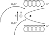 |
Fig. 10 Illustrative trajectories of gyrating protons and pick-up water ions, explaining the observed flow directions in the May–June 2015 period. Ions starting out in the middle of the two-dimensional sketch would go on the side (out of the plane) of the obstacle and not show a consistent pattern in the data. |
5 Conclusions
Our aim was to study the transition of the solar wind–comet interaction from sub-ion–gyroradius interaction at low-to-intermediate activity to a more fluid-like state at a high comet activity. The former is characterised by solar wind deflection culminating in sunward flows at a comet activity of about 1027 s−1. At a somewhat higher activity, the proton flow evolved to a consistent pattern with sunward H+ flows for zCSE > 0 and anti-sunward flows for zCSE < 0. This corresponds to a spatial flow pattern with simple trochoid trajectories in a relatively steep density gradient. At the inner edge of such flow trajectories, the solar wind ions move towards the Sun when closest to the nucleus for zCSE > 0 and anti-sunward for zCSE < 0. There is also a distinct solar wind ion cavity at this somewhat higher comet activity where the solar wind ions have time and room to perform multiple gyrations. The solar wind ion cavity is asymmetric, with a larger extent in the zCSE < 0 hemisphere. For the same somewhat higher activity, pick-up ions show a clear hemispheric asymmetry in relation to the solar wind electric field direction. For zCSE > 0 they move against the electric field, and for zCSE < 0 they move along the electric field. This is consistent with where ions picked up well upstream of the nucleus would be closest to the nucleus in the two electric field hemispheres as illustrated in Fig. 10.
The solar wind ions are slowed down more the closer they are to perihelion, reaching down to less than 50 km/s bulk velocity during the dayside excursion, with a comet activity of 1028 s−1. The H+ energy spectra are wide compared to what is seen throughout the mission in general, with a median one-dimensional H+ temperature of about 10–20 eV, as compared to 2 eV for the whole mission. This is consistent with a shock upstream of the observation point and later gradual slowing down as observed at more active comets. At the inner edge of the solar wind ion flow where observations were made, the solar wind ions are a minor species at a fraction of up to 10−3 of the ion density. Instead, pick-up ions at an energy level above 60 eV dominate the flux and sometimes the density of ions. The ion flow around 67P is more fluid-like closer to perihelion, with both solar wind and water ions collected upstream performing several gyrations within the near-comet environment, and the gyroradii of both species being smaller than the comet–spacecraft distance, and thus smaller than the comet’s magnetosphere.
Acknowledgements
The data used in this research is publicly available through ESA’s Planetary Science Archive (PSA) at https://archives.esac.esa.int/psa/ftp/INTERNATIONAL-ROSETTA-MISSION/. The work of CSW was funded by the Austrian Science Fund (FWF) 10.55776/P35954. The work of HN and AM was funded by the Swedish National Space Agency through grant 132/19.
References
- Acton Jr, C. H. 1996, Planet. Space Sci., 44, 65 [CrossRef] [Google Scholar]
- Acton, C., Bachman, N., Semenov, B., & Wright, E. 2018, Planet. Space Sci., 150, 9 [Google Scholar]
- Alho, M., Wedlund, C. S., Nilsson, H., et al. 2019, A&A, 630, A45 [NASA ADS] [CrossRef] [EDP Sciences] [Google Scholar]
- Alho, M., Jarvinen, R., Simon Wedlund, C., et al. 2021, MNRAS, 506, 4735 [NASA ADS] [CrossRef] [Google Scholar]
- Amata, E., Formisano, V., Cerulli-Irelli, R., et al. 1986, in ESLAB Symposium on the Exploration of Halley’s Comet, 250 [Google Scholar]
- Annex, A. M., Pearson, B., Seignovert, B., et al. 2020, J. Open Source Softw., 5, 2050 [CrossRef] [Google Scholar]
- Balsiger, H., Altwegg, K., Bühler, F., et al. 1986, Nature, 321, 330 [NASA ADS] [CrossRef] [Google Scholar]
- Behar, E. 2018, PhD thesis, Luleå University of Technology, Space Technology, Sweden [Google Scholar]
- Behar, E., Lindkvist, J., Nilsson, H., et al. 2016, A&A, 596, A42 [NASA ADS] [CrossRef] [EDP Sciences] [Google Scholar]
- Behar, E., Nilsson, H., Alho, M., Goetz, C., & Tsurutani, B. 2017, MNRAS, 469, S396 [Google Scholar]
- Behar, E., Tabone, B., Saillenfest, M., et al. 2018, A&A, 620, A35 [NASA ADS] [CrossRef] [EDP Sciences] [Google Scholar]
- Bergman, S., Stenberg Wieser, G., Wieser, M., Johansson, F. L., & Eriksson, A. 2020, JGR: Space Phys., 125, e2020JA027870 [Google Scholar]
- Berčič,, L., Behar, E., Nilsson, H., et al. 2018, A&A, 613, A57 [NASA ADS] [CrossRef] [EDP Sciences] [Google Scholar]
- Biermann, L., Brosowski, B., & Schmidt, H. U. 1967, Solar Phys., 1, 254 [NASA ADS] [CrossRef] [Google Scholar]
- Bockelée-Morvan, D., & Biver, N. 2017, Phil. Trans. Royal Soc. A: Math., Phys. Eng. Sci., 375, 20160252 [Google Scholar]
- Burch, J., Goldstein, R., Cravens, T., et al. 2007, SSR, 128, 697 [Google Scholar]
- Carr, C., Cupido, E., Lee, C. G. Y., et al. 2007, Space Sci Rev., 128, 629 [NASA ADS] [CrossRef] [Google Scholar]
- Coates, A., Johnstone, A., Kessel, R., et al. 1990, JGR: Space Phys., 95, 20701 [Google Scholar]
- Cravens, T., & Gombosi, T. 2004, Adv. Space Res., 33, 1968 [Google Scholar]
- Deca, J., Divin, A., Henri, P., et al. 2017, Phys. Rev. Lett., 118, 205101 [Google Scholar]
- Deca, J., Divin, A., Stephenson, P., et al. 2025, Planet. Space Sci., 258, 106064 [Google Scholar]
- Edberg, N. J. T., Alho, M., André, M., et al. 2016, MNRAS, 462, S45 [NASA ADS] [CrossRef] [Google Scholar]
- Edberg, N. J. T., Eriksson, A. I., Vigren, E., et al. 2019, ApJ, 158, 71 [Google Scholar]
- Edberg, N. J., Eriksson, A. I., Vigren, E., et al. 2024, A&A, 682, A51 [NASA ADS] [CrossRef] [EDP Sciences] [Google Scholar]
- Eriksson, A. I., Boström, R., Gill, R., et al. 2007, Space Sci. Rev., 128, 729 [Google Scholar]
- Formisano, V., Amata, E., Cattaneo, M., Torrente, P., & Johnstone, A. 1990, A&A, 238, 401 [Google Scholar]
- Fränz, M., Dubinin, E., Roussos, E., et al. 2006, SSR, 126, 165 [Google Scholar]
- Galand, M., Héritier, K. L., Odelstad, E., et al. 2016, MNRAS, 462, S331 [Google Scholar]
- Glassmeier, K.-H., Boehnhardt, H., Koschny, D., Kührt, E., & Richter, I. 2007a, SSR, 128, 1 [Google Scholar]
- Glassmeier, K.-H., Richter, I., Diedrich, A., et al. 2007b, SSR, 128, 649 [Google Scholar]
- Goetz, C., Gunell, H., Johansson, F., et al. 2021, Ann. Geophys., 39, 379 [NASA ADS] [CrossRef] [Google Scholar]
- Goetz, C., Volwerk, M., Richter, I., & Glassmeier, K.-H. 2017, MNRAS, 469, S268 [NASA ADS] [CrossRef] [Google Scholar]
- Goetz, C., Koenders, C., Hansen, K. C., et al. 2016, MNRAS, 462, S459 [NASA ADS] [CrossRef] [Google Scholar]
- Gringauz, K., Gombosi, T., Tátrallyay, M., et al. 1986, GRL, 13, 613 [Google Scholar]
- Gulkis, S., Allen, M., von Allmen, P., et al. 2015, Science, 347 [Google Scholar]
- Gunell, H., Goetz, C., Simon Wedlund, C., et al. 2018, A&A, 619, L2 [NASA ADS] [CrossRef] [EDP Sciences] [Google Scholar]
- Hansen, K. C., Altwegg, K., Berthelier, J.-J., et al. 2016, MNRAS, 462, S491 [Google Scholar]
- Huang, Z., Tóth, G., Gombosi, T. I., et al. 2018, MNRAS, 475, 2835 [NASA ADS] [CrossRef] [Google Scholar]
- Johnstone, A. D., Coates, A. J., Huddleston, D. E., et al. 1993, A&A, 273 [Google Scholar]
- Koenders, C., Goetz, C., Richter, I., Motschmann, U., & Glassmeier, K.-H. 2016, MNRAS, 462, S235 [Google Scholar]
- Mandt, K. E., Eriksson, A., Edberg, N. J. T., et al. 2016, MNRAS, 462, S9 [Google Scholar]
- Moeslinger, A., Wieser, G. S., Nilsson, H., et al. 2023, JGR: Space Phys., 128, e2022JA031082 [Google Scholar]
- Moeslinger, A., Gunell, H., Nilsson, H., Fatemi, S., & Stenberg Wieser, G. 2024, JGR: Space Phys., 129, e2024JA032757 [Google Scholar]
- Myllys, M., Henri, P., Galand, M., et al. 2019, A&A, 630, A42 [NASA ADS] [CrossRef] [EDP Sciences] [Google Scholar]
- Neugebauer, M., Neubauer, F. M., Balsiger, H., et al. 1987, GRL, 14, 995 [Google Scholar]
- Neubauer, F., Marschall, H., Pohl, M., et al. 1993, A&A, 268, L5 [Google Scholar]
- Nilsson, H. 2021, RPC-ICA User Guide v1.5, Tech. rep., European Space Agency [Google Scholar]
- Nilsson, H., Lundin, R., Lundin, K., et al. 2007, SSR, 128, 671 [Google Scholar]
- Nilsson, H., Stenberg Wieser, G., Behar, E., et al. 2015, Science, 347, aaa0571 [NASA ADS] [CrossRef] [Google Scholar]
- Nilsson, H., Stenberg Wieser, G., Behar, E., et al. 2017, MNRAS, 469, S252 [Google Scholar]
- Nilsson, H., Gunell, H., Karlsson, T., et al. 2018, A&A, 616, A50 [NASA ADS] [CrossRef] [EDP Sciences] [Google Scholar]
- Nilsson, H., Williamson, H., Bergman, S., et al. 2020, MNRAS, 498, 5263 [NASA ADS] [CrossRef] [Google Scholar]
- Ogino, T., Walker, R. J., & Ashour-Abdalla, M. 1988, JGR: Space Phys., 93, 9568 [Google Scholar]
- Reme, H., Mazelle, C., d’Uston, C., et al. 1994, JGR: Space Phys., 99, 2301 [Google Scholar]
- Rubin, M., Combi, M., Daldorff, L., et al. 2014, ApJ, 781, 86 [NASA ADS] [CrossRef] [Google Scholar]
- Rubin, M., Altwegg, K., Balsiger, H., et al. 2019, MNRAS, 489, 594 [Google Scholar]
- Stenberg Wieser, G., Odelstad, E., Wieser, M., et al. 2017, MNRAS, 469, S522 [NASA ADS] [CrossRef] [Google Scholar]
- Szegö, K., Glassmeier, K.-H., Bingham, R., et al. 2000, SSR, 94, 429 [Google Scholar]
- Tátrallyay, M., Szegö, K., Verigin, M., & Remizov, A. 1995, Adv. Space Res., 16, 35 [Google Scholar]
- Taylor, M. G. G. T., Altobelli, N., Buratti, B. J., & Choukroun, M. 2017, Phil. Trans. Royal Soc. A: Math., Phys. Eng. Sci., 375 [Google Scholar]
- Trotignon, J. G., Michau, J. L., Lagoutte, D., et al. 2007, SSR, 128, 713 [Google Scholar]
- Volwerk, M., Goetz, C., Behar, E., et al. 2019, A&A, 630, A44 [NASA ADS] [CrossRef] [EDP Sciences] [Google Scholar]
- Williamson, H., Nilsson, H., Stenberg Wieser, G., et al. 2020, GRL, 47, e2020GL088666 [Google Scholar]
- Williamson, H., Nilsson, H., Stenberg Wieser, G., Moeslinger, A., & Goetz, C. 2022, A&A, 660, A103 [NASA ADS] [CrossRef] [EDP Sciences] [Google Scholar]
- Williamson, H. N., Johansson, A., Canu-Blot, R., et al. 2024, MNRAS, 533, 1442 [Google Scholar]
- Wilson III, L. B., Brosius, A. L., Gopalswamy, N., et al. 2021, Rev. Geophys., 59, e2020RG000714 [NASA ADS] [CrossRef] [Google Scholar]
Appendix A Investigation of cross-talk
By selecting restricted mass channel and energy channel ranges after manual inspection, the dataset used here should have a very high reliability. Still we do see a weak proton signal at the same energies and same direction as a much stronger heavy ion signal. We therefore did a further check of whether the signal in the proton channels could be due to cross-talk from the heavier ion mass channels. Figure A.1 shows the occurrence of different counts in the heavy ion mass channels as function of energy for cases with no H+ signal (to the left) and with H+ signal (to the right). Each time, energy and directional anode (sector) is treated as an individual data point, there is no binning. If the H+ signal was mainly due to cross-talk, high heavy counts would be associated with H+ counts greater than zero. The opposite is seen. The highest heavy counts occur for cases with no H+ signal. Note that all H+ energy and mass channels were used, not just the manually selected ranges as described in Sect. 2.3 and Fig. 2.
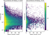 |
Fig. A.1 Occurrence (colour scale) of heavy ion counts (x axis) at different energies (y-axis). Left: Data when no signal was detected in the H+ mass channels at the same energy and for the same directional anode (sector). Right: Same but when the H+ signal was greater than zero. |
All Tables
Plasma parameters for three different regions divided into two hemispheres corresponding to the sign of zCSE.
All Figures
|
Fig. 1 One-dimensional distribution functions for H+ (red) and He2+ (blue). Solid lines show measurements, and dotted lines show Maxwellian distributions with the temperature and drift velocity as calculated from numerical integration of the observations. |
| In the text | |
|
Fig. 2 Screenshot from energy-mass channel-selection script. The user draws a box and identifies the ion species for any significant signal. Selected data are shown with a red box for H+, a blue box for He2+, and a green box for He+. Two red lines delineate the expected position of the H+ signal; a blue line shows the border between He2+ and He+. The colour-scale shows the logarithm of the number of counts. The shown signal is summed over all directions. |
| In the text | |
|
Fig. 3 Cometocentric distance of Rosetta (km) as function of time is shown with a black line (right y-axis). The mean speed of the observed solar wind protons (km/s on the right y-axis) is shown with occurrence in time-velocity bins using a colour-scale. The four periods discussed in the text are marked with numbers in the top of the plot. The beginning of the data, from 28 May 2015, is marked with an arrow. |
| In the text | |
|
Fig. 4 Overview of data from 28 May 2015. In all panels, the x-axis shows the time (UT). Top three panels: differential flux integrated over all observed angles using a colour-scale (cm−2 s−1 eV−1) with particle energy (eV) on the y-axis: electrons (panel a), water ions (panel b), and protons (panel c). Panel d: magnetic field components in the CSEQ coordinate system (nT). Thick lines are averaged over one ICA scan of 192 s. Panel e: proton velocity in the CSE reference frame (km/s). In both cases, dark blue is used for x, red for y, and orange for z. Panel f: integrated temperature estimates for protons. The one-dimensional temperature is shown in dark blue, and the three-dimensional temperature is given in orange. See the text for details on temperature calculations. Panel g: position of Rosetta in the y–z plane, with the distance along the magnetic field direction (CSE y) in dark blue and the distance along the electric field (CSE z) in orange (km). |
| In the text | |
|
Fig. 5 Proton observations in CSE y–z plane (circles). The colour of the circles indicates the mean particle speed with sign from the x component of the velocity moment (km/s). The size of the circle is a linear function of the of the density. The sizes corresponding to 0.01 and 1 cm−3 are shown in the lower right. |
| In the text | |
|
Fig. 6 Magnetic field observations in the y–z plane (circles). The colours of the circles show the magnitude of the magnetic field (nT) with sign from the Bx component. The sizes corresponding to 5 and 50 nT are shown in the lower right. |
| In the text | |
|
Fig. 7 Histograms of proton speed observed close to the nucleus (upper panels) in May and June 2015 (middle panels) and during the dayside excursion (lower panels). Left panels: velocity along the electric field component in the y–z plane. Right panels: sunward velocity (km/s). Brown indicates data for positive zCSE, and blue–green indicates data for negative zCSE. |
| In the text | |
|
Fig. 8 Left: occurrence frequency of solar wind observations (green line, lower x-axis), and total number of observations (black line, upper x-axis). Data are from periods 1 and 4 of Fig. 3, but at the beginning and end of the solar wind ion cavity. Right: zoomed-in view of Fig. 5 with the same zCSE axis as the left panel. The colour shows the speed of H+ with a sign from vx. |
| In the text | |
|
Fig. 9 Histograms of H2O+ speed observed close to the nucleus (upper panels) in May and June 2015 (middle panels) and during the dayside excursion (lower panels). Left panels: velocity along the electric field component in the y–z plane. Right panels: sunward velocity (km/s). Brown indicates data for positive zCSE, and blue-green indicates data for negative zCSE. |
| In the text | |
|
Fig. 10 Illustrative trajectories of gyrating protons and pick-up water ions, explaining the observed flow directions in the May–June 2015 period. Ions starting out in the middle of the two-dimensional sketch would go on the side (out of the plane) of the obstacle and not show a consistent pattern in the data. |
| In the text | |
|
Fig. A.1 Occurrence (colour scale) of heavy ion counts (x axis) at different energies (y-axis). Left: Data when no signal was detected in the H+ mass channels at the same energy and for the same directional anode (sector). Right: Same but when the H+ signal was greater than zero. |
| In the text | |
Current usage metrics show cumulative count of Article Views (full-text article views including HTML views, PDF and ePub downloads, according to the available data) and Abstracts Views on Vision4Press platform.
Data correspond to usage on the plateform after 2015. The current usage metrics is available 48-96 hours after online publication and is updated daily on week days.
Initial download of the metrics may take a while.