| Issue |
A&A
Volume 708, April 2026
|
|
|---|---|---|
| Article Number | A153 | |
| Number of page(s) | 14 | |
| Section | Extragalactic astronomy | |
| DOI | https://doi.org/10.1051/0004-6361/202555035 | |
| Published online | 03 April 2026 | |
Can a time-evolving, asymmetric broad line region mimic a massive black hole binary?
1
Università degli Studi di Milano-Bicocca, Piazza della Scienza 3, I-20126, Milano, Italy
2
SISSA – International School for Advanced Studies, Via Bonomea 265, I-34136, Trieste, Italy
3
INAF – Osservatorio Astronomico di Brera, Via Brera 20, I-20121, Milano, Italy
4
INFN, Sezione di Milano-Bicocca, Piazza della Scienza 3, I-20126, Milano, Italy
5
Como Lake centre for AstroPhysics (CLAP), DiSAT, Università dell’Insubria, Via Valleggio 11, 22100, Como, Italy
6
Department of Astronomy and Astrophysics and Institute for Gravitation and the Cosmos, Penn State University, 525 Davey Lab, 251 Pollock Road, University Park, PA, 16802, USA
★ Corresponding author: This email address is being protected from spambots. You need JavaScript enabled to view it.
Received:
4
April
2025
Accepted:
23
February
2026
Abstract
Gas within the influence sphere of accreting massive black holes is responsible for the emission of the broad lines observed in optical-UV spectra of unobscured active galactic nuclei. Since the region contributing the most to the broad emission lines (i.e. the broad line region) depends on the active galactic nucleus luminosity, the study of broad line reverberation to a varying continuum can map the morphology and kinematics of gas at sub-pc scales. In this study, we modify a preexisting model for disc-like broad line regions, including non-axisymmetric structures, by adopting an emissivity profile that mimics the observed luminosity-radius relation. This makes our implementation particularly well suited for the analysis of multi-epoch spectroscopic campaigns. After validating the model, we use it to check if strongly non-axisymmetric, single broad line regions could mimic the short time-scale evolution expected from massive black hole binaries. We explore different orientations and anisotropy degrees of the broad line region, as well as different light curve patterns of the continuum to which the broad line region responds. Our analysis confirms that recently proposed algorithms designed to search for massive black hole binaries in large multi-epoch spectroscopic data are not contaminated by false positives ascribed to anisotropic broad line regions around single massive black holes.
Key words: techniques: spectroscopic / galaxies: active / galaxies: interactions / quasars: emission lines / quasars: supermassive black holes
© The Authors 2026
 Open Access article, published by EDP Sciences, under the terms of the Creative Commons Attribution License (https://creativecommons.org/licenses/by/4.0), which permits unrestricted use, distribution, and reproduction in any medium, provided the original work is properly cited.
This article is published in open access under the Subscribe to Open model. This email address is being protected from spambots. You need JavaScript enabled to view it. to support open access publication.
1. Introduction
Super massive black hole binaries (SMBHBs) are expected to form during galaxy mergers (Begelman et al. 1980), and are expected to be the loudest sources of gravitational waves detectable in the nanohertz to millihertz frequency range (see Amaro-Seoane et al. 2017, 2023; Verbiest et al. 2016; EPTA Collaboration, InPTA Collaboration 2023; Agazie et al. 2023; Reardon et al. 2023; Xu et al. 2023). Due to the small separations at which a super massive black hole binary (SMBHB) forms (≈0.5 pc for a binary with total mass MSMBHB = 106 M⊙, see e.g. Dotti et al. 2012), resolving a binary (under the assumption that both super massive black holes (SMBHs) are active) is extremely challenging. Effectively, this prevents any instrument from directly inferring, through imaging, the binary nature of an active galactic nucleus (AGN). Indeed, only one candidate has been identified through resolved radio imaging (see Rodriguez et al. 2009), justifying the active search for alternative ways to reveal SMBHB signatures (see e.g. Popović 2012; De Rosa et al. 2019; Bogdanović et al. 2022, for a comprehensive overview of the possible methods attempted so far). Still, SMBHB signatures have been quite elusive because of the lack of unambiguous smoking guns demonstrating their effect on the electromagnetic (EM) radiation produced by an AGN. Indeed, the observational features used to identify SMBHB candidates, including periodic continuum variability and shifted-asymmetric broad emission lines (BELs), can also be generated by AGNs powered by single SMBHs (e.g. Vaughan et al. 2016; Liu et al. 2016; Dotti et al. 2022). In many cases, long-term observations (performed over a period longer than the alleged orbital period of the binary candidate) can rule out false positives (i.e. single SMBHs mimicking binary candidates). Unfortunately, the lengths of the observations required do not allow such a test. For this reason Dotti et al. (2023b) quantitatively study at length an alternative criterion, originally presented in a qualitative form in Gaskell (1988), for the identification of sub-parsec binaries with orbital periods of ≳10 − 100 yr, for which long-term monitoring covering many orbital periods is challenging or unfeasible. This criterion is based on the uncorrelated variability of the broad line regions (BLRs), when they are still retained by each individual SMBH in the binary. Due to the Doppler shift associated with their orbital motions, each BLR preferentially contributes to different velocities in the observed BEL profiles. A cross-correlation study of the blue and red sides of BELs therefore allows for the identification of (or validation of otherwise identified) SMBHB candidates, since in the binary case no correlation is predicted, while for single SMBHs high correlation is expected.
In this paper, we check if the proposed method can give false positives (i.e. identify single SMBHs as binaries) when a single BLR is sufficiently non-axisymmetric. In this situation, the BLR elements that contribute the most to the blue side of BELs (i.e. those moving towards the observer) can lie at different radii and react with different delays to variations of the continuum with respect to the gas contributing to the red side of the BEL. In order to verify the robustness of the observational test proposed in Dotti et al. (2023b) and summarized in Sect. 2, we model a single disc-like BLR featuring a non-axisymmetric perturbation based on the framework proposed by Storchi-Bergmann et al. (2003). Building on that formalism and to maximize the realism of our model, we further modified the existing prescription to include the continuum luminosity dependence of the BLR radius (see, e.g. Kaspi et al. 2000; Bentz et al. 2009). Specifically, our work is divided as follows. In Sect. 2 we construct the model to reproduce the flux associated with the specific system described above. In Sect. 3, we verify the physical consistency of our model with the observational results obtained from reverberation mapping (RM) campaigns, and then we conduct a thorough parameter exploration to test the robustness of the observational test proposed in Dotti et al. (2023b). Finally, we draw our main conclusion in Sect. 4.
2. Methodology
2.1. Geometry and coordinate system
We assume a razor-thin, disc-like BLR geometry whose reference frame has been chosen as shown in Fig. 1 (see also Chen et al. 1989). Here, the observer’s line is parallel to the z′ axis inclined by angle i from the z axis in the direction of the negative x axis. The BLR disc major axis as seen by the observer is aligned with the y-axis, while the angle ϕ is computed starting from the disc minor axis as seen by the observer. The central object is assumed to be a black hole of mass M = 108 M⊙1 and it is located in the common origin of the reference systems. The disc is parametrized by an inner and an outer radius ξ1 and ξ2 where the dimensionless radius ξ, defined as ξ = r/rG with rG = GM/c2, has been used to facilitate analysis2.
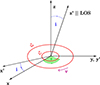 |
Fig. 1. Geometry and coordinate systems used for the model (see also Chen et al. 1989). ξ1 and ξ2 are respectively the inner and outer radius of the BLR, while i is the inclination. The angle ϕ is measured counter-clockwise from the near side of the disc. |
2.2. Continuum luminosity
The BLR elements respond to continuum variations with an average light-travel-time (LTT) delay, τLTT. The average delay is obtained from the time lag between fluctuations of the continuum and the integrated flux of an emission line. This delay is used to estimate the ‘characteristic’ size of the BLR RBLR = c τLTT (see Blandford & McKee 1982; Peterson 1993). To test the physical consistency of the proposed emissivity profile (Sect. 2.3) we studied the BLR response to different continuum variations which we model by letting the intrinsic luminosity of the central SMBH change with time. Specifically, to test different scenarios we studied the BLR reaction to an intrinsic luminosity parametrized by a step-function
 (1)
(1)
and a sinusoid
 (2)
(2)
where 𝒯 = 40 d for the step function and 𝒯 = 120 d for the sinusoidal continuum3., while the normalizations of the two light curves are completely arbitrary, as well as the total luminosity emitted by the BLR. In this study, we stick to simple analytic functions to simplify the interpretation of the results. However, more realistic light curves are used in Appendix C to show that our results do not depend on the simple analytical parametrization of the light curves assumed.
2.3. BLR emissivity
As discussed above, we tested the robustness of the Dotti et al. (2023b) test when applied to a single disc-like BLR with strong non-axisymmetric perturbations. We assumed a modified version of the formulation proposed by Gilbert et al. (1999) and Storchi-Bergmann et al. (2003) for the line emissivity (i.e. emitted flux)
![Mathematical equation: $$ \begin{aligned} \begin{split} \epsilon (\xi , \phi ; \xi _{\rm c}, { w};\boldsymbol{u}) = \epsilon _0&\ \xi ^{-1}\exp \left[-\frac{(\xi -\xi _{\rm c})^2}{2w^2}\right]\biggl \{1 +\\ &\frac{A}{2}\exp \left[-\frac{4\ln {2}}{\delta ^2}\biggl (\phi - \psi _0(\xi )\biggr )^2\right]+\\&\frac{A}{2}\exp \left[-\frac{4\ln {2}}{\delta ^2}\biggl (2\pi - \phi + \psi _0(\xi )\biggr )^2\right]\biggr \}, \end{split} \end{aligned} $$](/articles/aa/full_html/2026/04/aa55035-25/aa55035-25-eq3.gif) (3)
(3)
where ϵ0 is a scale factor with units of erg per second per square centimeter. The first term characterizes the axisymmetric part of the emissivity, while the other terms represent the deviation from axisymmetry caused by a perturbation with the form of a spiral arm4. Here, we define the array u = [A, δ, ϕ0, p], which represents the set of the spiral arm parameters.
The angular dependent part of Eq. (3) is identical to the original Storchi-Bergmann et al. (2003) proposal, where the second and third Gaussians are used to represent the decay of the emissivity of the spiral arm with azimuthal distance on either side of the ridge line, while the parameter A modulates the brightness contrast between the spiral arm and the Gaussian emissivity underneath. The parameter δ is for the azimuthal full width at half maximum (FWHM) of the spiral arm, while the value ϕ − ψ0 denotes the azimuthal distance from the ridge of the spiral arm, defined by the following
 (4)
(4)
with p and ξsp describing, respectively, the winding rate and the innermost radius of the spiral arm, while ϕ0 portrays the azimuthal orientation of the spiral pattern.
Instead, we modified the radial dependence of the emissivity to incorporate the observational relation between the characteristic radius of the BLR (RBLR) and the central source luminosity obtained by reverberation mapping campaigns (see Kaspi et al. 2000). In particular, we assumed the scaling discussed in Bentz et al. (2009)
 (5)
(5)
where fEdd is the accretion bolometric luminosity normalized to the Eddington limit. The radial profile chosen in Eq. (3) ensures that the emissivity centred radius ξc obeys approximately the observed luminosity–radius relation in Eq. (5)5, as long as it behaves accordingly to the following dependence on the continuum luminosity
![Mathematical equation: $$ \begin{aligned} \xi _{\rm c} (t_{\mathrm{obs}}) = \xi _{\rm c,0}\cdot \left(\frac{\mathcal{L} \left[t^{\prime }(t_{\mathrm{obs}}, \xi , \phi )\right]}{\mathcal{L} _0}\right)^{0.5}. \end{aligned} $$](/articles/aa/full_html/2026/04/aa55035-25/aa55035-25-eq6.gif) (6)
(6)
In the above equation ξc, 0 is the dimensionless average radius, ℒ0 is the average luminosity, t′ is defined as
![Mathematical equation: $$ \begin{aligned} t\prime = t_{\rm obs} - \xi \left[ \frac{r_{G}}{c} \cdot (1 + \sin {i} \cdot \cos {\phi })\right] \end{aligned} $$](/articles/aa/full_html/2026/04/aa55035-25/aa55035-25-eq7.gif) (7)
(7)
to take into account the delayed response time for each BLR element, and tobs is the observation time. As a result of the above definitions, ξc is an implicit function of tobs. The width in the Gaussian term, w, is assumed to be equal to w = ξc/26.
In Appendix A, we show how the BLR brightness changes with different combinations of the spiral arm parameters, while an application on real data is presented in Rigamonti et al. (2025).
2.4. Local Doppler shift and broadening
After establishing the BLR emissivity, we take into account the effect of the local BLR bulk motion and turbulence on the Doppler shift and broadening of the emission line profiles. As the BLR rotates around the z-axis (see Fig. 1), the observer will perceive an increased or decreased frequency, depending on whether the emitting region is approaching or receding from them. Assuming the BLR elements to be on Keplerian circular orbits, the line-of-sight velocity is given by Eq. (8):
 (8)
(8)
Then, for the specific intensity of the line (in units of erg s−1 cm−2 Å−1 sterad−1), we adopted the prescription proposed by Chen et al. (1989) and Chen & Halpern (1989)
![Mathematical equation: $$ \begin{aligned} \begin{split} I_{\lambda } =\frac{\epsilon (\xi ,\phi ; \xi _{\rm c}, { w};\boldsymbol{u})}{4\pi }&\cdot \frac{\mathcal{L} \left[t\prime (t_{\mathrm{obs}}, \xi , \phi )\right]}{\mathcal{L} _0}\cdot \\&\cdot \frac{1}{\sqrt{2\pi }\sigma _\lambda }\exp \left[-\frac{(\lambda - \lambda _{\rm e}\cdot (1+v_{\mathrm{obs}}/c))^2}{2\sigma _\lambda ^2}\right], \end{split} \end{aligned} $$](/articles/aa/full_html/2026/04/aa55035-25/aa55035-25-eq9.gif) (9)
(9)
where ϵ(ξ, ϕ; ξc, w; u) is the emissivity defined by Eq. (3), ℒ[t′(tobs,ξ,ϕ)]/ℒ0 represents the apparent luminosity pattern of the disc by the continuum source, which sets the local effective emissivity. Local broadening is included as a Gaussian profile with a broadening parameter σλ set to 1200 km/s in the model, as in the original Storchi-Bergmann et al. (2003) implementation. In the following analysis, we model the response of the Hα line, but the same test can be performed for different BELs as long as the model parameters are properly adapted. Therefore, the wavelength of the line in the emitter frame is set to λe = 6563 Å. Finally, we stress that the line intensity profile in Eq. (9) has an explicit dependence on the impinging continuum luminosity, to allow the BEL to increase or decrease its luminosity in response to the continuum modulations.
We note that not all the relativistic processes considered in the previous implementations (e.g. Chen & Halpern 1989; Chen et al. 1989) have been taken into account in the current model. In particular, the effect of gravitational redshift, light bending, and any effect associated with radiative transfer processes within the BLR are not taken into consideration at the current stage. A brief comparison with a similar implementation that includes such effects is presented in Appendix B. Although such effects have a small influence on the line profiles, they do not influence the results of the test we perform in this work.
2.5. Binary test through cross-correlation analysis
From an observational point of view, the measurement of the BLR physical size utilizes a collection of several spectra taken at different times that contain at least one BEL. The time delay between the AGN continuum and the reprocessed light from the BLR is typically estimated by comparing their respective light curves. There are multiple approaches to efficiently estimate such time delays efficiently (Peterson et al. 2004; Pancoast et al. 2014; Zu et al. 2011; Raimundo et al. 2020; Donnan et al. 2021; Pozo Nuñez et al. 2023). Most of them, such as the method of Peterson et al. (2004) employed here, are based on the maximization of the cross-correlation between the two light curves.
Dotti et al. (2023b) proposed a test that, by exploiting RM observations, identifies SMBHBs at separations large enough for the two SMBHs to still retain their individual BLR (i.e. each BLR is small enough to fit inside their Roche lobes). In our methodology (dubbed fast uncorrelated variability test, FUVT) the variable part of a broad emission line is divided into eight equal flux wavelength bins separated by seven  . For each of the
  we divide the spectrum of the selected BEL into a red and blue component (for wavelengths longer and shorter than
  , respectively). We then compute the light curves of these components, perform the cross-correlation between the two, and measure the maximum cross-correlation for each
  and the associated time shift (see Dotti et al. 2023a, for further details). At this point, if the cross-correlation is low for all
  (especially for those concentrated near the bulk of the line where S/N is not likely to adversely affect the measurement), there might be an indication of the presence of a SMBHB. Indeed, in the case of two detached BLRs orbiting around the common centre of mass of the system, it is expected that each one of them predominantly contributes to the red or blue light curve. Moreover, since the two BLRs are reprocessing the light coming from two different ionizing sources, their red and blue light curves will show much less correlation compared to the case of a single SMBH. In Appendix C we show the comparison between the expected results for both a single SMBH and a SMBHB scenario.
3. Results
In this section, we show how the line profile at each time and its overall time evolution depend on the parameters assumed for the BLR emissivity. Subsequently, we will focus on the cross-correlation analysis presented above, performed using the PYTHON adaptation (see Sun et al. 2018) of the code originally developed by Peterson et al. (2004). We first check the ability of our implementation to reproduce the luminosity–radius relation by computing the cross-correlation between the total flux of the BEL and the continuum. Then, we compute the cross-correlation between the red part and the blue part of the line for a statistically relevant number of BLR profiles, to test whether the method could wrongly associate with these scenarios the presence of a SMBHB in the context of the FUVT described above.
3.1. Emission line profiles
The upper left panel of Fig. 2 shows the Hα BEL for different sets of emissivity parameters (listed in the upper right corner of the figure) under the assumption of a sinusoidal variation of the continuum (see Eq. (2)). Each emission line represents the same snapshot (i.e. the flux is taken at the same time of observation). As expected, the spiral perturbation introduces asymmetries in the emission line profile based on its different properties. As seen in Fig. 2, we allow the parameter A to vary up to 100. This approach enables us to evaluate the reliability of the FUVT by considering also a strongly non-axisymmetric BLR. However, we stress that these values are higher than the ones used to fit observed line profiles. For instance, in Storchi-Bergmann et al. (2017) and Ward et al. (2024) reasonable fits to observed line profiles are obtained constraining A to values below 10. Hence, we extend the variation of A up to 100 to test the reliability of FUVT under extreme conditions.
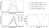 |
Fig. 2. Example of line profiles. In the first row, different BELs obtained at the same time of observation (tobs = 0) for different sets of parameters (listed on the upper right legend). In the second row, the evolution of the BEL obtained by the fourth set of parameters (i.e. the ones associated with the red emission profile in the first row) is shown at different observation times (left) with the corresponding centroid (right). |
In the second row of Fig. 2, we fix the BLR parameters to those identified by the red colour in the legend and show the evolution of the BEL as a function of time (i.e. from tobs = 0 to tobs = 150 d). Specifically, the bottom left panel shows the line profile at six different snapshots reported in the panel legend. As seen in this panel, the height of the profile varies with observation time. This happens because, in our model, the line profile is linearly dependent on the continuum, here assumed to be a sinusoidal continuum with a period of 𝒯 = 120 d. Therefore, the profile follows a similar behaviour. On the bottom right panel, we report the evolution with time of the line centroid computed by considering the median wavelength at which the line is split into two equal flux regions7. As noted in the introduction, the presence of an asymmetric BEL with line centroid (either the peak or flux weighted wavelength) shifted with respect to the host redshift has been used as a tool to identify SMBHB candidates (see, e.g. Tsalmantza et al. 2011; Eracleous et al. 2012, for examples of systematic searches). The shift of the line centroid in time can be used to distinguish between false binary candidates and true SMBHBs (e.g. Decarli et al. 2013; Runnoe et al. 2015, 2017). The example in Fig. 2 demonstrates that small shifts in the BEL centroid can be obtained even with a single SMBH irradiating a single non-axisymmetric BLR. However, these shifts are of the order of a few hundred kilometers−1 and would tend to introduce noise (‘jitter’) in the long-term radial velocity curves that track the line peak, as discussed in Runnoe et al. (2017). In the following, we demonstrate that for large separation binaries, as the one considered in the current study, the test proposed in Dotti et al. (2023a) can distinguish between single and binary SMBHs, while at smaller separations ad-hoc tests must be devised to prevent the misidentification of single SMBHs as binaries, as discussed in Bertassi et al. (2025).
Finally, in Fig. 3 we show the intrinsic emissivity map ϵ(ξ, ϕ; ξc, w; u) for this set of parameters, the instantaneous illumination pattern for the sinusoidal input light curve (i.e. ℒ(t′) where t′ is given by Eq. (7)) and their corresponding product, which is the instantaneous brightness map (i.e. the input to the line profile computation) at a fixed observation time tobs = 0 d. This illustrates how the system responds to the ionizing continuum.
 |
Fig. 3. Illustration of how the disc responds to the variable ionizing continuum for the set of parameters A = 95, δ = 10°, ϕ0 = 96° and p = 25°. The line of sight is assumed to be inclined by i = 30° with respect to the normal to the disc in the direction of the negative x-axes. From left to right: The intrinsic emissivity map, the instantaneous illumination map, and the instantaneous brightness map. As can be noted, the impact of ℒ(t′) leads at the assumed time (tobs = 0) to a greater enhancement of the BLR emissivity on the near side (i.e. closer to the observer) compared to the far side. |
3.2. Reverberation mapping: Continuum versus total integrated flux of the BEL
Here, we show how well our model is able to reproduce the luminosity–radius relation obtained through reverberation mapping campaigns. To test our model, we first fixed the spiral parameters at constant values reported in Table 1, along with the fixed values of the inclination, and inner and outer radii of the disc.
BLR parameters for consistency check.
We let ξc, 0 vary between ξ1 and ξ28. For each value of ξc, 0, we computed the line profile for 200 different observational times between 0 and t = 150 d. We then used them to construct the light curve for the total integrated line flux. Finally, we calculated the cross-correlation between the integrated line and the continuum considering both the step function and the sinusoidal continuum (Figs. 4 and 5, respectively). In both figures we show from top to bottom: the continuum luminosity (either Eq. (1) or Eq. (2)), the corresponding BEL response, and the cross-correlation between the continuum and the integrated line as a function of time. In the bottom panel the vertical blue line represents the time delay that maximizes the cross-correlation (τcc), while the red line shows the average time delay (τweight), estimated as the centroid of the cross-correlation function (CCF) based on all points with correlation coefficients exceeding a threshold equal to 0.8τcc, following the convention adopted by Peterson et al. (1998). As can be observed by the legend reported in the panel, the two methods give consistent results. The time delays are then used to compute RBLR.
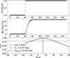 |
Fig. 4. Cross-correlation analysis, assuming a step function continuum (i.e. Eq. (1)). On the upper panel, the continuum luminosity. On the middle panel, the total integrated fluxes of a BEL. Finally, on the lower panel, the cross-correlation computations. |
In Fig. 6 we show the characteristic size of the BLR estimated from the cross-correlation analysis for both the step function and the sinusoidal continuum. The circular and triangular shapes refer to the specific approach considered for estimating the characteristic size of the BLR (maximum or weighted average, respectively), while the different colours represent different continuum light curves. In particular, blue and orange markers are used for the step function continuum, while red and green markers are associated with the sinusoidal continuum. The uncertainties considered in Fig. 6 are estimated from the discrete set of time delays evaluated, taken as the spacing between consecutive delay values. The additional vertical and horizontal axes report the time delays in units of days.
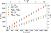 |
Fig. 6. Comparison between the characteristic radius of the BLR obtained by applying reverberation mapping techniques and the radius obtained from the luminosity–radius relation. We show with blue and orange markers the results from the step-function continuum luminosity, while we use green and red markers for the sinusoidal continuum. In both cases, the radius has been estimated considering the maximum of the cross-correlation (represented by circular markers), as well as the weighted average of the time delays (represented by a triangular markers) (see Sect. 3 for further details). |
As seen in Fig. 6, the values obtained for the sinusoidal continuum are always higher with respect to those of the step function. Our analysis shows that the exact value of the ratio between the characteristic size of the BLR obtained through the reverberation mapping and the emissivity averaged radius ξc, 0 depends on the time-evolution of the continuum. This result is already known, and it is discussed from an analytical point of view in Krolik (2001). Nonetheless, we find a linear relation between RBLR and ξc, 0. Such a linear scaling maps into the expected dependence of RBLR and the continuum luminosity, allowing for the use of the BLR model introduced for the analysis of multi-epoch spectra.
3.3. Reliability of the FUVT in the asymmetric BLR scenario
Once we verified the physical consistency of our model, in order to investigate the robustness of the FUVT method, we computed the cross-correlation between the blue and red fluxes of the emission line for a large number of different BLR scenarios. Specifically, contrary to what was done in Sect. 3.1, we fixed ξc, 0 = 1200, considered the sinusoidal continuum, and let the spiral parameters vary, creating 104 different BLR configurations corresponding to 104 BEL profiles. We assumed the parameter ranges to be δ, ϕ0 ∈ [0, 2π], p ∈ [ − π/2, π/2], and A ∈ [0, 100], respectively.9 As mentioned earlier, the broader range for A with respect to the one resulting from fits of the observed line profile is chosen to account for strongly non-axisymmetric BLR, allowing us to test the FUVT reliability under these extreme scenarios as well. For each BLR profile, we first computed the line profile for 175 equally-spaced times between tobs = 0 and tobs = 150 d. Due to the high number of scenarios to be processed, we used an NVIDIA TESLA P100 GPU – provided by Kaggle10 – to optimize the efficiency of our code by parallelizing the generation of fluxes. This approach allowed us to generate 175 line profiles (i.e. one scenario) in 6 seconds. On a standard CPU (i.e. AMD Ryzen 7 3700U), the same computation is performed in 7 minutes.
Following Dotti et al. (2023b), we determine the cross-correlation dependence on the wavelength at which the division of the line is performed, as summarized in Sect. 2.5. An example of the seven distinct cross-correlation values obtained for the set of BLR parameters presented in Table 2 is shown in Fig. 811.
BLR parameters for noise.
For each BLR profile, we considered the maximum value obtained for the cross-correlation to analyse the predictions that would be obtained from the method. As can be seen from the corner plot shown in Fig. 7, all scenarios returned a maximum for the cross-correlation on the order of unity, with a minimum value given by min(CCF) = 0.9962.
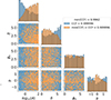 |
Fig. 7. Pairplot showing the cross-correlation value distribution in the spiral arm parameters space. The obtained values are always higher than min(CCF) = 0.9962. Thus, the cross-correlation consistently approaches a value close to unity. We categorized the data into two classes, using the median value as the cut-off. |
At this stage, the reliability of the FUVT in the asymmetric BLR scenario has been studied assuming a sinusoidal continuum, which does not reflect the observed AGN variability. However, we recover the consistent results with a more realistic continuum, such as a damped random walk (see Appendix C). As our intent is to verify the impact of the intrinsic properties of the BLR on the red-blue cross-correlation, we worked under the assumption of zero uncertainties on the BEL profiles. However, as discussed in Dotti et al. (2023b), observational errors in the data might reduce the red-blue cross-correlation, both for observations of single or binary systems. A detailed study of the effect of noise is the topic of a follow-up study (Bertassi et al., in prep.). Here we show only an example of the same analysis discussed above, in which we assumed the BLR parameters in Table 2 and ξc, 0 = 1200, and we added to the resulting BEL profile different levels of Gaussian noise.
Specifically, at each time and for each wavelength we added to the flux predicted by the BLR model an independent sampling from a Gaussian centred at 0 and with different values of s, as illustrated in the left panel of Fig. 8 for tobs = 0. The cross-correlation between the blue and the red part of the BEL is then computed as in the previous (noiseless) case. As shown in the right panel of Fig. 8, the value of the cross-correlation is indeed modified by the addition of the noise, with the profile of CCF as a function of the BEL cut becoming similar to the one observed in most of the single SMBH cases analysed in Dotti et al. (2023b): the CCF remains high (≳0.8) when dividing the BEL in two close-to-equal-flux parts, while it decreases significantly towards no correlation when one side of the line accounts for a small fraction of the overall flux and is, therefore, strongly affected by the noise.
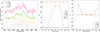 |
Fig. 8. On the left panel, noise implementation on the profile obtained using the set of parameters listed in Table 2 and the sinusoidal continuum given by Eq. (2) at tobs = 0. Here, we assume Gaussian noise with different values for s, as indicated in the inset. To highlight the effect of the applied Gaussian noise, each BEL is shown with a vertical offset. We stress that only the BEL is plotted, while an AGN spectrum in the broad Hα spectral region would feature, at the very least, the AGN and the host galaxy continua. The negative values of the flux are therefore not unphysical, and should be interpreted as uncertainties on the total (positive) flux. On the central panel, CCF results as a function of the noise. The value of the cross-correlation decreases as the amplitude of the noise increases. The maximum of the cross-correlation remains higher than 0.8 for all the cases considered, in which s remains smaller than the peak value of the BEL flux. On the right panel, time delays corresponding to the time shifts that maximize the correlation coefficient. Note that for asymmetric flux divisions (e.g., a blue fraction of 0.1 or 0.9), the resulting time delays deviate from values close to zero. This occurs because the code was allowed to shift the blue and red part of the BELs over a broader range than what is physically expected. As the flux contributions from the blue and red components become comparable, the time delay that maximizes the cross-correlation coefficient naturally returns to values near zero, as expected. |
4. Discussion and conclusions
The aim of this work is to check whether the FUVT test originally proposed by Gaskell (1988) and developed by Dotti et al. (2023b) is capable of correctly recognizing a single SMBH in the presence of a non-axisymmetric BLR. To do this, we modelled the continuum impinging on the BLR through analytical functions, either a step function or a sinusoid (Eqs. (1) and (2), respectively). We generated a disc-like BLR characterized by a spiral arm perturbation on an otherwise radial emissivity, whose profile ensures that the characteristic radius corresponds to the expectations from the observed luminosity–radius relation. The BEL profile has been shaped in wavelengths by the leading order Doppler shift associated with the local bulk velocity of each BLR element, and a local broadening associated to unresolved turbulence. Although we neglected any relativistic effects, we compared our model with a similar implementation that takes into account gravitational redshift, light bending, and any effect associated with radiative transfer processes, as described in Ogborn et al. (2025). As we show in Appendix B, the most significant impact on the line profile is a shift of the spectrum towards higher wavelengths, with the blue peak increasing in height and the red peak decreasing. Since the relativistic effects on the line profile shape seem to be small, we believe that these differences do not compromise the results of our test, hence validating the robustness and reliability of FUVT.
We validated the model by testing whether it is capable of approximately reproducing the luminosity-radius relation described by Eq. (5). We stress that, to date, ours is the first implementation encoding directly into the model the BEL response due to the luminosity–radius relation to a time dependent continuum.
After testing the physical consistency of our model, we checked the robustness of the method proposed by Dotti et al. (2023b). We thoroughly explored the parameter space of our model by varying the parameters of the spiral arm and computing the corresponding cross-correlation between the red part and the blue part of the resulting line. Our results rule out the possibility that spiral-like asymmetric BLRs can be mistaken by the FUVT as SMBHBs. We emphasize that the results presented in this paper are based on a sinusoidal continuum and assume both perfect time sampling and noise-free data. In Appendix C, we also show results for a more realistic underlying continuum. A detailed study of the effect of noise is the topic of a follow-up study (Bertassi et al., in prep.). All the different scenarios used to check the robustness of the test were characterized by a value for the cross-correlation between the red part and the blue part of the line on the order of unity, which corresponds to a correct identification of the presence of a single SMBH. The robustness of FUVT can be further tested, for example, by modifying the BLR model, either changing the BLR dynamics (e.g. considering an eccentric disc, as in Eracleous et al. 1995) or including additional relativistic effects shaping the fine details of the BEL profile as in Chen et al. (1989) and Chen & Halpern (1989) (see also Appendix B). However, the results obtained from this study are promising with respect to the identification of SMBHBs in RM.
Acknowledgments
ES acknowledges Kaggle for providing access to their platform computational resources, including GPU support. MD acknowledges support from ICSC – Centro Nazionale di Ricerca in High Performance Computing, Big Data and Quantum Computing, funded by European Union – NextGenerationEU, and the Italian Ministry for Research and University (MUR) under Grant ‘Progetto Dipartimenti di Eccellenza 2023-2027’ (BiCoQ). FR acknowledges the support from the Next Generation EU funds within the National Recovery and Resilience Plan (PNRR), Mission 4 – Education and Research, Component 2 – From Research to Business (M4C2), Investment Line 3.1 – Strengthening and creation of Research Infrastructures, Project IR0000012 – “CTA+ – Cherenkov Telescope Array Plus. M.E. acknowledges support from the U.S. National Science Foundation under award number 2205720. M.O. acknowledges support from the U.S. National Science Foundation under award number 2205720, and the Pennsylvania State Science Achievement Graduate Fellowship Program. MB acknowledges support provided by MUR under grant “PNRR – Missione 4 Istruzione e Ricerca – Componente 2 Dalla Ricerca all’Impresa – Investimento 1.2 Finanziamento di progetti presentati da giovani ricercatori ID:SOE_0163” and by University of Milano-Bicocca under grant “2022-NAZ-0482/B”. MB acknowledges support from the Italian Ministry for Universities and Research (MUR) program “Dipartimenti di Eccellenza 2023-2027”, within the framework of the activities of the Centro Bicocca di Cosmologia Quantitativa (BiCoQ). FR acknowledges support from ELSA. ELSA Euclid Legacy Science Advanced analysis tools” (Grant Agreement no. 101135203) is funded by the European Union. Views and opinions expressed are, however, those of the author(s) only and do not necessarily reflect those of the European Union or Innovate UK. Neither the European Union nor the granting authority can be held responsible for them.
References
- Agazie, G., Anumarlapudi, A., Archibald, A. M., et al. 2023, ApJ, 951, L8 [NASA ADS] [CrossRef] [Google Scholar]
- Amaro-Seoane, P., Andrews, J., Arca Sedda, M., et al. 2023, Liv. Rev. Relat., 26, 2 [NASA ADS] [CrossRef] [Google Scholar]
- Amaro-Seoane, P., Audley, H., Babak, S., et al. 2017, ESA, submitted [arXiv:1702.00786] [Google Scholar]
- Begelman, M. C., Blandford, R. D., & Rees, M. J. 1980, Nature, 287, 307 [Google Scholar]
- Bentz, M. C., Peterson, B. M., Netzer, H., Pogge, R. W., & Vestergaard, M. 2009, ApJ, 697, 160 [Google Scholar]
- Bertassi, L., Sottocorno, E., Rigamonti, F., et al. 2025, A&A, 702, A165 [NASA ADS] [CrossRef] [EDP Sciences] [Google Scholar]
- Blandford, R. D., & McKee, C. F. 1982, ApJ, 255, 419 [Google Scholar]
- Bogdanović, T., Miller, M. C., & Blecha, L. 2022, Liv. Rev. Relat., 25, 3 [Google Scholar]
- Chen, K., & Halpern, J. P. 1989, ApJ, 344, 115 [NASA ADS] [CrossRef] [Google Scholar]
- Chen, K., Halpern, J. P., & Filippenko, A. V. 1989, ApJ, 339, 742 [NASA ADS] [CrossRef] [Google Scholar]
- De Rosa, A., Vignali, C., Bogdanović, T., et al. 2019, New Astron. Rev., 86, 101525 [Google Scholar]
- Decarli, R., Dotti, M., Fumagalli, M., et al. 2013, MNRAS, 433, 1492 [Google Scholar]
- Donnan, F. R., Horne, K., & Hernández Santisteban, J. V. 2021, MNRAS, 508, 5449 [NASA ADS] [CrossRef] [Google Scholar]
- Dotti, M., Sesana, A., & Decarli, R. 2012, Adv. Astron., 2012, 940568 [CrossRef] [Google Scholar]
- Dotti, M., Bonetti, M., D’Orazio, D. J., Haiman, Z., & Ho, L. C. 2022, MNRAS, 509, 212 [Google Scholar]
- Dotti, M., Bonetti, M., Rigamonti, F., et al. 2023a, MNRAS, 518, 4172 [Google Scholar]
- Dotti, M., Rigamonti, F., Rinaldi, S., et al. 2023b, A&A, 680, A69 [NASA ADS] [CrossRef] [EDP Sciences] [Google Scholar]
- EPTA Collaboration, InPTA Collaboration, Antoniadis, J., et al. 2023, A&A, 678, A50 [CrossRef] [EDP Sciences] [Google Scholar]
- Eracleous, M., Halpern, L., & Storchi-Bergmann, T. 1995, ApJ, 438, 610 [NASA ADS] [CrossRef] [Google Scholar]
- Eracleous, M., Boroson, T. A., Halpern, J. P., & Liu, J. 2012, ApJS, 201, 23 [Google Scholar]
- Gaskell, C. M. 1988, in Active Galactic Nuclei, eds. H. R. Miller, & P. J. Wiita, 307, 61 [Google Scholar]
- Gilbert, A. M., Eracleous, M., Filippenko, A. V., & Halpern, J. P. 1999, ASP Conf. Ser., 175, 189 [Google Scholar]
- Kaspi, S., Smith, P. S., Netzer, H., et al. 2000, ApJ, 533, 631 [Google Scholar]
- Kelly, B. C., Bechtold, J., & Siemiginowska, A. 2009, ApJ, 698, 895 [Google Scholar]
- Krolik, J. H. 2001, ApJ, 551, 72 [NASA ADS] [CrossRef] [Google Scholar]
- Liu, T., Gezari, S., Burgett, W., et al. 2016, ApJ, 833, 6 [NASA ADS] [CrossRef] [Google Scholar]
- Ogborn, M., Eracleous, M., Runnoe, J. C., et al. 2025, ApJS, accepted [arXiv:2511.17334] [Google Scholar]
- Pancoast, A., Brewer, B. J., Treu, T., et al. 2014, MNRAS, 445, 3073 [Google Scholar]
- Peterson, B. M. 1993, PASP, 105, 247 [NASA ADS] [CrossRef] [Google Scholar]
- Peterson, B. M., Wanders, I., Horne, K., et al. 1998, PASP, 110, 660 [Google Scholar]
- Peterson, B. M., Ferrarese, L., Gilbert, K. M., et al. 2004, ApJ, 613, 682 [Google Scholar]
- Popović, L. Č. 2012, New Astron. Rev., 56, 74 [Google Scholar]
- Pozo Nuñez, F., Gianniotis, N., & Polsterer, K. L. 2023, A&A, 674, A83 [NASA ADS] [CrossRef] [EDP Sciences] [Google Scholar]
- Raimundo, S. I., Vestergaard, M., Goad, M. R., et al. 2020, MNRAS, 493, 1227 [Google Scholar]
- Reardon, D. J., Zic, A., Shannon, R. M., et al. 2023, ApJ, 951, L6 [NASA ADS] [CrossRef] [Google Scholar]
- Rigamonti, F., Severgnini, P., Sottocorno, E., et al. 2025, A&A, 693, A117 [NASA ADS] [CrossRef] [EDP Sciences] [Google Scholar]
- Rodriguez, C., Taylor, G. B., Zavala, R. T., Pihlström, Y. M., & Peck, A. B. 2009, ApJ, 697, 37 [NASA ADS] [CrossRef] [Google Scholar]
- Runnoe, J. C., Eracleous, M., Mathes, G., et al. 2015, ApJS, 221, 7 [NASA ADS] [CrossRef] [Google Scholar]
- Runnoe, J. C., Eracleous, M., Pennell, A., et al. 2017, MNRAS, 468, 1683 [Google Scholar]
- Storchi-Bergmann, T., Nemmen da Silva, R., Eracleous, M., et al. 2003, ApJ, 598, 956 [NASA ADS] [CrossRef] [Google Scholar]
- Storchi-Bergmann, T., Schimoia, J. S., Peterson, B. M., et al. 2017, ApJ, 835, 236 [Google Scholar]
- Sun, M., Grier, C. J., & Peterson, B. M. 2018, Astrophysics Source Code Library [record ascl:1805.032] [Google Scholar]
- Tsalmantza, P., Decarli, R., Dotti, M., & Hogg, D. W. 2011, ApJ, 738, 20 [Google Scholar]
- Vaughan, S., Uttley, P., Markowitz, A. G., et al. 2016, MNRAS, 461, 3145 [Google Scholar]
- Verbiest, J. P. W., Lentati, L., Hobbs, G., et al. 2016, MNRAS, 458, 1267 [Google Scholar]
- Ward, C., Gezari, S., Nugent, P., et al. 2024, ApJ, 961, 172 [NASA ADS] [CrossRef] [Google Scholar]
- Xu, H., Chen, S., Guo, Y., et al. 2023, Res. Astron. Astrophys., 23, 075024 [CrossRef] [Google Scholar]
- Zu, Y., Kochanek, C. S., & Peterson, B. M. 2011, ApJ, 735, 80 [NASA ADS] [CrossRef] [Google Scholar]
The results can be scaled for different SMBH masses, by rescaling the properties of the BLR and the luminosity of the accreting SMBH.
Henceforth, to differentiate between the dimensionless radius and the actual radius, we denote them as ξ and r.
This period was chosen to be smaller in both cases than the observational times considered in Sect. 3 (set to tobs ∈ [0, 150] d).
Note that the third term is identical to the second term shifted by 2π. This term is required to enforce periodicity and to avoid discontinuities around ϕ = 0, 2π.
Note that we approximated the exponent of the luminosity in Eq. (5) to 0.5.
Note that the centroid shifts up or down in wavelength as the line integrated flux increases or decreases, respectively.
Recall that ξ1 and ξ2 are the inner and outer radii of the disc-like BLR.
Specifically, the distributions for δ, ϕ0, and p are all uniform, while a log-uniform distribution is used for A.
Precisely, the s = 0 scenario.
This number of sections is specifically due to the GPU memory limits.
Appendix A: Emissivity parameters
In this Appendix we show how the BLR brightness changes with the parameters of the spiral arm model.
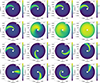 |
Fig. A.1. Effect of the emissivity parameters on the BLR emissivity pattern. Each row underline the effects of an increasing A, δ, ϕ0 and p respectively. The parameter in the legend is the only one varying along the row, while the others are kept constant to the following value: A = 100 and δ, ϕ0, p = 20°. For each configuration, we use ξc = 1200 and w = ξc/2 = 600. |
Appendix B: Model comparison
In this Appendix, we compare the results of our model - hereafter referred to as Sottocorno’s Model (SM) - with those obtained by a model that involves an expansion at leading order of different relativistic effects. In particular, while we consider only the Doppler effect, the model (referred to as OM in the following) presented in Ogborn et al. (2025) also includes gravitational redshift, Doppler boosting and transverse redshift. In particular, the OM model includes the same relativistic effects as the model of Chen et al. (1989) and Chen & Halpern (1989), except light bending which is negligible. To illustrate the impact of relativistic effects, we consider two different scenarios: one with no spiral arm (A = 0) and another with a spiral arm (A = 2). The corresponding parameters are shown in Tab. B.1 and Tab. B.2 respectively. Both the comparisons were done by considering a constant luminosity, so that the brightness and emissivity patterns are exactly the same.
BLR parameters for model comparison (A = 0).
BLR parameters for model comparison (A = 2).
In our implementation, we divide the BLR into 175 annuli and 175 azimuths and compute their contributions to the total spectrum for 175 wavelengths12. In contrast, OM uses 1000 × 1000 sections to describe the BLR and computes the spectrum for 1000 wavelengths. Additionally, while both models use a polar coordinate system, the SM employs a grid that is linear in both azimuth and radius, whereas the OM model applies a logarithmic scale to the radius while keeping azimuth linear. Therefore, we also compare the spectra obtained considering only the Doppler effect for both models in order to highlight the underlying differences due to the different model resolutions as well.
To give a quantitative measure of the differences, we relied on the following properties: first, we computed the first and second moments for each spectrum, given by:
 (B.1)
(B.1)
respectively. We then converted them into units of km/s:
 (B.2)
(B.2)
where we recall that λe = 6563 Å. Then we compared the relative heights of the two peaks and their corresponding distances, which we defined respectively as:
 (B.3)
(B.3)
In order to facilitate the comparison, we normalized the spectra so that the underlying area for each spectrum is equal to unity in both scenarios.
Firstly, we show in Fig. B.1 the spectra obtained for the scenario without a spiral arm and in Tab. B.3 and Tab. B.4 the resulting properties.
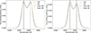 |
Fig. B.1. Comparison between the spectra obtained for the BLR without a spiral arm. On the left, both models include only the Doppler effect; on the right, OM also considers relativistic effects. |
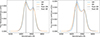 |
Fig. B.2. Comparison between the spectra obtained for the BLR with a spiral arm. On the left, both models include only the Doppler effect; on the right, OM also considers relativistic effects. |
Property comparison (A = 0, only Doppler).
Property comparison (A = 0, relativistic effects).
Property comparison (A = 2, only Doppler).
Property comparison (A = 2, relativistic effects).
As we can see, while the scenario with only the Doppler effect included for both models remains comparable, the inclusion of relativistic effects causes a shift towards higher wavelengths and alters the relative height of the two peaks. Specifically, the blue peak becomes more pronounced, while the red peak diminishes. This results in a higher relative height compared to the scenario considering only the Doppler effects. This also leads to a shift in the computed centroid, while the standard deviation and the peaks separation are barely affected.
Then, we show in Fig. B.2 the spectra obtained for the scenario with a spiral arm and in Tab. B.5 and Tab. B.6 the resulting properties.
As we can see, also in this case the inclusion of relativistic effects causes a shift towards higher wavelengths and modifies the relative height of the two peaks, while the two models remain comparable if considering only the Doppler effect. Since the impact of relativistic effects on the spectrum is comparable to that described in the previous cases, this also results in a higher relative height compared to the scenario considering only Doppler effects and a shift in the computed centroid. However, in this case, we also observe that the differences in both the standard deviation and the peak distances diminish.
Our tests confirm that including relativistic effects does not affect our results or change the conclusions of the FUVT test on the data. The key findings remain consistent in both cases, showing that while relativistic corrections exist, they are only a second-order effect and do not significantly influence the overall outcome of the test.
Appendix C: Realistic scenario and binary comparison
Here, we briefly present the results obtained when adopting a more realistic prescription for the intrinsic light curve. Specifically, we replaced the theoretical luminosity in Eq. 2 with a damped random walk (DRW), a stochastic process commonly used to model AGN variability with red-noise behaviour (see Kelly et al. 2009). Additionally, we include the results obtained by modeling a simulated binary system, which we used as a basis for comparison with the other scenarios.
To generate the DRW variabilities, we assumed a mean value of μ = 14 and a characteristic timescale of τDRW = 100 d for both the light curves, while we considered for the fluctuation amplitude σDRW = [0.08, 0.12], respectively. In Fig.C.1 we show the resulting realizations.
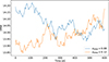 |
Fig. C.1. DRW variability used for the realistic scenario and the binary comparison. The blue light curve and the orange light curve correspond to the scenario with σDRW = 0.08, σDRW = 0.12 respectively. The mean value and the characteristic timescale are fixed to μ = 14 and τ = 100 d for both cases. |
Once we derived the light curves, we repeated the same procedure described in Sect. 2.5 to compute the CCF between the blue part and the red part of the BEL. As it can be seen in Fig. C.2, even in this case the CCF remains higher than 0.9, leading to unity, with the FUVT correctly identifying this scenario as a single SMBH independently on the light curve assumed.
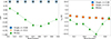 |
Fig. C.2. On the left panel, CCF results for two single SMBHs and a simulated binary given by the spectra presented in Fig. C.3, as a function of different fractions of the total BEL luminosity in the blue part of the line. On the right panel, the corresponding time delays, i.e. the time shifts that maximize the correlation coefficient. Since the BLR extends from 200 − 1800 rG ∼ 1 − 10 ld, the expected delays between the blue part and the red part of the line are of order of only a few days. The monotonic decrease of the time delay with respect to the blue fraction in the single SMBH case reflects that the line wings, which arise at smaller radii, respond faster. To better visualize this shorter delays, the right panel is shown with a restricted vertical range (−10 to 10 d). |
Additionally, we compared these results with those obtained assuming the presence of a SMBHB, by using the two different DRW realizations to mimic a BEL generated by a binary. To do that, we computed the spectrum using the two light curves separately, assuming no spiral arm (A = 0) and an inclination i = 10° for the BLR disc in order to obtain two single peak profiles. Then, following Dotti et al. (2023b), we shifted the resulting BELs by 30 Å each in opposite directions to mimic the presence of a binary and selected the BLR parameters for the single SMBH (listed in Tab. C.1) so that the binary and single SMBH spectra would closely resemble each other under the two realistic continua.
BLR parameters (vrel ≃ 5485 km/s).
In Fig. C.3 we show both the shift process and the comparison with the more realistic single SMBHs obtained by using the DRWs lightcurves.
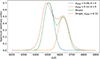 |
Fig. C.3. Example of a simulated binary spectrum and comparison with the double peaked single SMBH spectrum obtained assuming a DRW continuum at tobs = 0. The spectra derived from the light curves in Fig. C.1 with A = 0 (no spiral arms) are shown in blue (σDRW = 0.08) and orange (σDRW = 0.12), while the resulting simulated binary spectrum is plotted in green. To construct the latter, the individual SMBH spectra were shifted to the blue and red by 30 Å each respectively. Additionally, the spectra obtained with the parameters listed in Tab. C.1 assuming a single SMBH and a DRW continuum are also plotted to show the resemblance with the binary BEL. |
Once we simulated the binary, we repeated the procedure described in Sect. 2.5 to compute the CCF between the red part and the blue part of the BEL. As can be seen from Fig. C.2, the CCF in this scenario clearly deviates from unity even in absence of measurement uncertainties, with the CCF showing a symmetric trend with respect to the blue fraction and a minimum when the BEL is divided such that the red part and the blue part contain an equal value of the integrated flux as also observed in Dotti et al. (2023b).
This drop is expected to occur because, when a binary has a large enough separation for each SMBH to maintain its own BLR, different portions of the BEL respond to different continuum sources. If the two SMBHs vary independently, the blue and red peaks evolve differently, leading to a low CCF. This effect is expected to be maximized when the BEL is split so that the blue side and the red side each isolate the flux originating from one SMBH (i.e. when the blue fraction is approximately 0.5-0.6 in our scenario).
However, we stress that the shift required to reproduce this profile corresponds to a relative velocity  , which is greater than the characteristic BLR velocity, except for nearly face on configurations. For this reason, we also present the results obtained using a more moderate shift, consistent with the assumption that both SMBHs can sustain their own BLR according to the FUVT requirements. In particular, we shifted the BELs obtained with i = 10° and A = 0 by 10 Å each in opposite directions, corresponding to a relative velocity of vrel ≃ 1830 km/s. This yields the single peak profile shown in Fig. C.4, which can still mimic that of a single SMBH with a non-axisymmetric BLR. For instance, with parameters presented in Tab. C.2 we retrieve a spectrum comparable with the binary one.
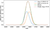 |
Fig. C.4. Example of a simulated binary spectrum and comparison with the double peaked single SMBH spectra obtained assuming a DRW continuum at tobs = 0. The spectra derived from the light curves in Fig. C.1 with A = 0 (no spiral arms) are shown in blue (σDRW = 0.08) and orange (σDRW = 0.12), while the resulting simulated binary spectrum is plotted in green. To construct the latter, the individual SMBH spectra were shifted to the blue and red by 10 Å each respectively. Additionally, the spectra obtained with the parameters listed in Tab. C.2 assuming a single SMBH and a DRW continuum are also plotted to show the resemblance with the binary BEL. |
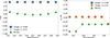 |
Fig. C.5. On the left panel, CCF results for two single SMBHs and a simulated binary given by the spectra presented in Fig. C.4, as a function of different fractions of the total BEL luminosity in the blue part of the line. On the right panel, the corresponding time delays, i.e. the time shifts that maximize the correlation coefficient. Here, the monotonic decrease is less evident than in Fig. C.2 since the measured delays are smaller than the adopted observational time step. |
BLR parameters ((vrel ≃ 1830 km/s).
Here again, we repeated the procedure described in Sect. 2.5 and computed the CCF between the red part and the blue part of the BEL, obtaining a similar result with respect to the double-peak scenario. In particular, altough the CCF becomes systematically higher across all blue fractions, it remains distinctly less than one. Furthermore, the same symmetric trend as before is preserved, with a minimum at the blue fraction that yields the greatest separation between the red and blue parts of the underlying BELs. We stress that we only proved that, for an extremely high SNR, the test proposed by Dotti et al. (2023b) cannot misidentify a single SMBH as a binary even for very asymmetric BLRs. Adding noise could decrease the observed correlation (as observed in Sect. 3, hence even if the test is robust against false positive, it cannot identify all binaries. Indeed, if the intrinsic ionizing continua of the two SMBHs have similar light curves, the test will recover a high correlation between the blue and the red BEL regions (see also Dotti et al. 2023b, for further details).
All Tables
All Figures
|
Fig. 1. Geometry and coordinate systems used for the model (see also Chen et al. 1989). ξ1 and ξ2 are respectively the inner and outer radius of the BLR, while i is the inclination. The angle ϕ is measured counter-clockwise from the near side of the disc. |
| In the text | |
|
Fig. 2. Example of line profiles. In the first row, different BELs obtained at the same time of observation (tobs = 0) for different sets of parameters (listed on the upper right legend). In the second row, the evolution of the BEL obtained by the fourth set of parameters (i.e. the ones associated with the red emission profile in the first row) is shown at different observation times (left) with the corresponding centroid (right). |
| In the text | |
|
Fig. 3. Illustration of how the disc responds to the variable ionizing continuum for the set of parameters A = 95, δ = 10°, ϕ0 = 96° and p = 25°. The line of sight is assumed to be inclined by i = 30° with respect to the normal to the disc in the direction of the negative x-axes. From left to right: The intrinsic emissivity map, the instantaneous illumination map, and the instantaneous brightness map. As can be noted, the impact of ℒ(t′) leads at the assumed time (tobs = 0) to a greater enhancement of the BLR emissivity on the near side (i.e. closer to the observer) compared to the far side. |
| In the text | |
|
Fig. 4. Cross-correlation analysis, assuming a step function continuum (i.e. Eq. (1)). On the upper panel, the continuum luminosity. On the middle panel, the total integrated fluxes of a BEL. Finally, on the lower panel, the cross-correlation computations. |
| In the text | |
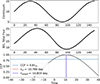 |
Fig. 5. Same as Fig. 4 assuming a sinusoidal continuum (i.e. Eq. (2)). |
| In the text | |
|
Fig. 6. Comparison between the characteristic radius of the BLR obtained by applying reverberation mapping techniques and the radius obtained from the luminosity–radius relation. We show with blue and orange markers the results from the step-function continuum luminosity, while we use green and red markers for the sinusoidal continuum. In both cases, the radius has been estimated considering the maximum of the cross-correlation (represented by circular markers), as well as the weighted average of the time delays (represented by a triangular markers) (see Sect. 3 for further details). |
| In the text | |
|
Fig. 7. Pairplot showing the cross-correlation value distribution in the spiral arm parameters space. The obtained values are always higher than min(CCF) = 0.9962. Thus, the cross-correlation consistently approaches a value close to unity. We categorized the data into two classes, using the median value as the cut-off. |
| In the text | |
|
Fig. 8. On the left panel, noise implementation on the profile obtained using the set of parameters listed in Table 2 and the sinusoidal continuum given by Eq. (2) at tobs = 0. Here, we assume Gaussian noise with different values for s, as indicated in the inset. To highlight the effect of the applied Gaussian noise, each BEL is shown with a vertical offset. We stress that only the BEL is plotted, while an AGN spectrum in the broad Hα spectral region would feature, at the very least, the AGN and the host galaxy continua. The negative values of the flux are therefore not unphysical, and should be interpreted as uncertainties on the total (positive) flux. On the central panel, CCF results as a function of the noise. The value of the cross-correlation decreases as the amplitude of the noise increases. The maximum of the cross-correlation remains higher than 0.8 for all the cases considered, in which s remains smaller than the peak value of the BEL flux. On the right panel, time delays corresponding to the time shifts that maximize the correlation coefficient. Note that for asymmetric flux divisions (e.g., a blue fraction of 0.1 or 0.9), the resulting time delays deviate from values close to zero. This occurs because the code was allowed to shift the blue and red part of the BELs over a broader range than what is physically expected. As the flux contributions from the blue and red components become comparable, the time delay that maximizes the cross-correlation coefficient naturally returns to values near zero, as expected. |
| In the text | |
|
Fig. A.1. Effect of the emissivity parameters on the BLR emissivity pattern. Each row underline the effects of an increasing A, δ, ϕ0 and p respectively. The parameter in the legend is the only one varying along the row, while the others are kept constant to the following value: A = 100 and δ, ϕ0, p = 20°. For each configuration, we use ξc = 1200 and w = ξc/2 = 600. |
| In the text | |
|
Fig. B.1. Comparison between the spectra obtained for the BLR without a spiral arm. On the left, both models include only the Doppler effect; on the right, OM also considers relativistic effects. |
| In the text | |
|
Fig. B.2. Comparison between the spectra obtained for the BLR with a spiral arm. On the left, both models include only the Doppler effect; on the right, OM also considers relativistic effects. |
| In the text | |
|
Fig. C.1. DRW variability used for the realistic scenario and the binary comparison. The blue light curve and the orange light curve correspond to the scenario with σDRW = 0.08, σDRW = 0.12 respectively. The mean value and the characteristic timescale are fixed to μ = 14 and τ = 100 d for both cases. |
| In the text | |
|
Fig. C.2. On the left panel, CCF results for two single SMBHs and a simulated binary given by the spectra presented in Fig. C.3, as a function of different fractions of the total BEL luminosity in the blue part of the line. On the right panel, the corresponding time delays, i.e. the time shifts that maximize the correlation coefficient. Since the BLR extends from 200 − 1800 rG ∼ 1 − 10 ld, the expected delays between the blue part and the red part of the line are of order of only a few days. The monotonic decrease of the time delay with respect to the blue fraction in the single SMBH case reflects that the line wings, which arise at smaller radii, respond faster. To better visualize this shorter delays, the right panel is shown with a restricted vertical range (−10 to 10 d). |
| In the text | |
|
Fig. C.3. Example of a simulated binary spectrum and comparison with the double peaked single SMBH spectrum obtained assuming a DRW continuum at tobs = 0. The spectra derived from the light curves in Fig. C.1 with A = 0 (no spiral arms) are shown in blue (σDRW = 0.08) and orange (σDRW = 0.12), while the resulting simulated binary spectrum is plotted in green. To construct the latter, the individual SMBH spectra were shifted to the blue and red by 30 Å each respectively. Additionally, the spectra obtained with the parameters listed in Tab. C.1 assuming a single SMBH and a DRW continuum are also plotted to show the resemblance with the binary BEL. |
| In the text | |
|
Fig. C.4. Example of a simulated binary spectrum and comparison with the double peaked single SMBH spectra obtained assuming a DRW continuum at tobs = 0. The spectra derived from the light curves in Fig. C.1 with A = 0 (no spiral arms) are shown in blue (σDRW = 0.08) and orange (σDRW = 0.12), while the resulting simulated binary spectrum is plotted in green. To construct the latter, the individual SMBH spectra were shifted to the blue and red by 10 Å each respectively. Additionally, the spectra obtained with the parameters listed in Tab. C.2 assuming a single SMBH and a DRW continuum are also plotted to show the resemblance with the binary BEL. |
| In the text | |
|
Fig. C.5. On the left panel, CCF results for two single SMBHs and a simulated binary given by the spectra presented in Fig. C.4, as a function of different fractions of the total BEL luminosity in the blue part of the line. On the right panel, the corresponding time delays, i.e. the time shifts that maximize the correlation coefficient. Here, the monotonic decrease is less evident than in Fig. C.2 since the measured delays are smaller than the adopted observational time step. |
| In the text | |
Current usage metrics show cumulative count of Article Views (full-text article views including HTML views, PDF and ePub downloads, according to the available data) and Abstracts Views on Vision4Press platform.
Data correspond to usage on the plateform after 2015. The current usage metrics is available 48-96 hours after online publication and is updated daily on week days.
Initial download of the metrics may take a while.