| Issue |
A&A
Volume 708, April 2026
|
|
|---|---|---|
| Article Number | A104 | |
| Number of page(s) | 40 | |
| Section | Extragalactic astronomy | |
| DOI | https://doi.org/10.1051/0004-6361/202555728 | |
| Published online | 30 March 2026 | |
Euclid preparation
LXXXVI. Cosmic Dawn Survey: Evolution of the galaxy stellar mass function across 0.2 < z ≤ 6.5 measured over 10 square degrees
1
Institute for Astronomy, University of Hawaii, 2680 Woodlawn Drive, Honolulu, HI 96822, USA
2
Department of Astronomy, University of Massachusetts, Amherst, MA 01003, USA
3
Cosmic Dawn Center (DAWN), Denmark
4
Niels Bohr Institute, University of Copenhagen, Jagtvej 128, 2200 Copenhagen, Denmark
5
Department of Astrophysical Sciences, Peyton Hall, Princeton University, Princeton, NJ 08544, USA
6
Physics and Astronomy Department, University of California, 900 University Ave., Riverside, CA 92521, USA
7
Caltech/IPAC, 1200 E. California Blvd., Pasadena, CA 91125, USA
8
Cosmic Dawn Center (DAWN)
9
ESAC/ESA, Camino Bajo del Castillo s/n., Urb. Villafranca del Castillo, 28692 Villanueva de la Cañada, Madrid, Spain
10
School of Mathematics and Physics, University of Surrey, Guildford, Surrey GU2 7XH, UK
11
INAF-Osservatorio Astronomico di Brera, Via Brera 28, 20122 Milano, Italy
12
INAF-Osservatorio di Astrofisica e Scienza dello Spazio di Bologna, Via Piero Gobetti 93/3, 40129 Bologna, Italy
13
IFPU, Institute for Fundamental Physics of the Universe, via Beirut 2, 34151 Trieste, Italy
14
INAF-Osservatorio Astronomico di Trieste, Via G. B. Tiepolo 11, 34143 Trieste, Italy
15
INFN, Sezione di Trieste, Via Valerio 2, 34127 Trieste TS, Italy
16
SISSA, International School for Advanced Studies, Via Bonomea 265, 34136 Trieste, TS, Italy
17
Dipartimento di Fisica e Astronomia, Università di Bologna, Via Gobetti 93/2, 40129 Bologna, Italy
18
INFN-Sezione di Bologna, Viale Berti Pichat 6/2, 40127 Bologna, Italy
19
INAF-Osservatorio Astrofisico di Torino, Via Osservatorio 20, 10025 Pino Torinese (TO), Italy
20
Dipartimento di Fisica, Università di Genova, Via Dodecaneso 33, 16146 Genova, Italy
21
INFN-Sezione di Genova, Via Dodecaneso 33, 16146 Genova, Italy
22
Department of Physics “E. Pancini”, University Federico II, Via Cinthia 6, 80126 Napoli, Italy
23
INAF-Osservatorio Astronomico di Capodimonte, Via Moiariello 16, 80131 Napoli, Italy
24
Instituto de Astrofísica e Ciências do Espaço, Universidade do Porto, CAUP, Rua das Estrelas, PT4150-762 Porto, Portugal
25
Faculdade de Ciências da Universidade do Porto, Rua do Campo de Alegre, 4150-007 Porto, Portugal
26
Aix-Marseille Université, CNRS, CNES, LAM, Marseille, France
27
Dipartimento di Fisica, Università degli Studi di Torino, Via P. Giuria 1, 10125 Torino, Italy
28
INFN-Sezione di Torino, Via P. Giuria 1, 10125 Torino, Italy
29
European Space Agency/ESTEC, Keplerlaan 1, 2201 AZ, Noordwijk, The Netherlands
30
Institute Lorentz, Leiden University, Niels Bohrweg 2, 2333 CA, Leiden, The Netherlands
31
INAF-IASF Milano, Via Alfonso Corti 12, 20133 Milano, Italy
32
Centro de Investigaciones Energéticas, Medioambientales y Tecnológicas (CIEMAT), Avenida Complutense 40, 28040 Madrid, Spain
33
Port d’Informació Científica, Campus UAB, C. Albareda s/n, 08193 Bellaterra (Barcelona), Spain
34
Institute for Theoretical Particle Physics and Cosmology (TTK), RWTH Aachen University, 52056 Aachen, Germany
35
Institute of Space Sciences (ICE, CSIC), Campus UAB, Carrer de Can Magrans, s/n, 08193 Barcelona, Spain
36
Institut d’Estudis Espacials de Catalunya (IEEC), Edifici RDIT, Campus UPC, 08860 Castelldefels, Barcelona, Spain
37
INAF-Osservatorio Astronomico di Roma, Via Frascati 33, 00078 Monteporzio Catone, Italy
38
INFN section of Naples, Via Cinthia 6, 80126 Napoli, Italy
39
Dipartimento di Fisica e Astronomia “Augusto Righi” – Alma Mater Studiorum Università di Bologna, Viale Berti Pichat 6/2, 40127 Bologna, Italy
40
Instituto de Astrofísica de Canarias, E-38205 La Laguna, Tenerife, Spain
41
Institute for Astronomy, University of Edinburgh, Royal Observatory, Blackford Hill, Edinburgh EH9 3HJ, UK
42
Jodrell Bank Centre for Astrophysics, Department of Physics and Astronomy, University of Manchester, Oxford Road, Manchester M13 9PL, UK
43
European Space Agency/ESRIN, Largo Galileo Galilei 1, 00044 Frascati, Roma, Italy
44
Université Claude Bernard Lyon 1, CNRS/IN2P3, IP2I Lyon, UMR 5822, Villeurbanne F-69100, France
45
Institut de Ciències del Cosmos (ICCUB), Universitat de Barcelona (IEEC-UB), Martí i Franquès 1, 08028 Barcelona, Spain
46
Institució Catalana de Recerca i Estudis Avançats (ICREA), Passeig de Lluís Companys 23, 08010 Barcelona, Spain
47
UCB Lyon 1, CNRS/IN2P3, IUF, IP2I Lyon, 4 rue Enrico Fermi, 69622 Villeurbanne, France
48
Departamento de Física, Faculdade de Ciências, Universidade de Lisboa, Edifício C8, Campo Grande, PT1749-016 Lisboa, Portugal
49
Instituto de Astrofísica e Ciências do Espaço, Faculdade de Ciências, Universidade de Lisboa, Campo Grande, 1749-016 Lisboa, Portugal
50
Department of Astronomy, University of Geneva, ch. d’Ecogia 16, 1290 Versoix, Switzerland
51
INAF-Istituto di Astrofisica e Planetologia Spaziali, Via del Fosso del Cavaliere 100, 00100 Roma, Italy
52
Université Paris-Saclay, CNRS, Institut d’astrophysique spatiale, 91405 Orsay, France
53
INFN-Padova, Via Marzolo 8, 35131 Padova, Italy
54
Aix-Marseille Université, CNRS/IN2P3, CPPM, Marseille, France
55
Université Paris-Saclay, Université Paris Cité, CEA, CNRS, AIM, 91191 Gif-sur-Yvette, France
56
Space Science Data Center, Italian Space Agency, via del Politecnico snc, 00133 Roma, Italy
57
INFN-Bologna, Via Irnerio 46, 40126 Bologna, Italy
58
School of Physics, HH Wills Physics Laboratory, University of Bristol, Tyndall Avenue, Bristol BS8 1TL, UK
59
Universitäts-Sternwarte München, Fakultät für Physik, Ludwig-Maximilians-Universität München, Scheinerstr. 1, 81679 München, Germany
60
Max Planck Institute for Extraterrestrial Physics, Giessenbachstr. 1, 85748 Garching, Germany
61
INAF-Osservatorio Astronomico di Padova, Via dell’Osservatorio 5, 35122 Padova, Italy
62
Herzberg Astronomy and Astrophysics Research Centre, 5071 W. Saanich Rd, Victoria, BC V9E 2E7, Canada
63
Institute of Theoretical Astrophysics, University of Oslo, P.O. Box 1029 Blindern 0315, Oslo, Norway
64
Jet Propulsion Laboratory, California Institute of Technology, 4800 Oak Grove Drive, Pasadena, CA 91109, USA
65
Department of Physics, Lancaster University, Lancaster LA1 4YB, UK
66
Felix Hormuth Engineering, Goethestr. 17, 69181 Leimen, Germany
67
Technical University of Denmark, Elektrovej 327, 2800 Kgs, Lyngby, Denmark
68
Max-Planck-Institut für Astronomie, Königstuhl 17, 69117 Heidelberg, Germany
69
NASA Goddard Space Flight Center, Greenbelt, MD 20771, USA
70
Department of Physics and Astronomy, University College London, Gower Street, London WC1E 6BT, UK
71
Department of Physics and Helsinki Institute of Physics, Gustaf Hällströmin katu 2, University of Helsinki, 00014 Helsinki, Finland
72
Leiden Observatory, Leiden University, Einsteinweg 55, 2333 CC, Leiden, The Netherlands
73
Université de Genève, Département de Physique Théorique and Centre for Astroparticle Physics, 24 quai Ernest-Ansermet, CH-1211 Genève 4, Switzerland
74
Department of Physics, P.O. Box 64, University of Helsinki, 00014 Helsinki, Finland
75
Helsinki Institute of Physics, Gustaf Hällströmin katu 2, University of Helsinki, 00014 Helsinki, Finland
76
Laboratoire Univers et Théorie, Observatoire de Paris, Université PSL, Université Paris Cité, CNRS, 92190 Meudon, France
77
SKAO, Jodrell Bank, Lower Withington, Macclesfield SK11 9FT, UK
78
Centre de Calcul de l’IN2P3/CNRS, 21 avenue Pierre de Coubertin, 69627 Villeurbanne Cedex, France
79
Dipartimento di Fisica “Aldo Pontremoli”, Università degli Studi di Milano, Via Celoria 16, 20133 Milano, Italy
80
INFN-Sezione di Milano, Via Celoria 16, 20133 Milano, Italy
81
Universität Bonn, Argelander-Institut für Astronomie, Auf dem Hügel 71, 53121 Bonn, Germany
82
INFN-Sezione di Roma, Piazzale Aldo Moro, 2 – c/o Dipartimento di Fisica, Edificio G. Marconi, 00185 Roma, Italy
83
Dipartimento di Fisica e Astronomia “Augusto Righi” – Alma Mater Studiorum Università di Bologna, via Piero Gobetti 93/2, 40129 Bologna, Italy
84
Department of Physics, Institute for Computational Cosmology, Durham University, South Road, Durham DH1 3LE, UK
85
Université Côte d’Azur, Observatoire de la Côte d’Azur, CNRS, Laboratoire Lagrange, Bd de l’Observatoire, CS 34229 06304 Nice cedex 4, France
86
Institut d’Astrophysique de Paris, UMR 7095, CNRS, and Sorbonne Université, 98 bis boulevard Arago, 75014 Paris, France
87
Université Paris Cité, CNRS, Astroparticule et Cosmologie, 75013 Paris, France
88
CNRS-UCB International Research Laboratory, Centre Pierre Binétruy, IRL2007, CPB-IN2P3 Berkeley, USA
89
Institut d’Astrophysique de Paris, 98bis Boulevard Arago, 75014 Paris, France
90
Institute of Physics, Laboratory of Astrophysics, Ecole Polytechnique Fédérale de Lausanne (EPFL), Observatoire de Sauverny, 1290 Versoix, Switzerland
91
Aurora Technology for European Space Agency (ESA), Camino bajo del Castillo s/n, Urbanizacion Villafranca del Castillo, Villanueva de la Cañada, 28692 Madrid, Spain
92
Institut de Física d’Altes Energies (IFAE), The Barcelona Institute of Science and Technology, Campus UAB, 08193 Bellaterra (Barcelona), Spain
93
School of Mathematics, Statistics and Physics, Newcastle University, Herschel Building, Newcastle-upon-Tyne, NE1 7RU, UK
94
DARK, Niels Bohr Institute, University of Copenhagen, Jagtvej 155, 2200 Copenhagen, Denmark
95
Centre National d’Etudes Spatiales – Centre spatial de Toulouse, 18 avenue Edouard Belin, 31401 Toulouse Cedex 9, France
96
Institute of Space Science, Str. Atomistilor, nr. 409 Măgurele, Ilfov 077125, Romania
97
Consejo Superior de Investigaciones Cientificas, Calle Serrano 117, 28006 Madrid, Spain
98
Universidad de La Laguna, Dpto. Astrofísica, E-38206 La Laguna, Tenerife, Spain
99
Dipartimento di Fisica e Astronomia “G. Galilei”, Università di Padova, Via Marzolo 8, 35131 Padova, Italy
100
Institut für Theoretische Physik, University of Heidelberg, Philosophenweg 16, 69120 Heidelberg, Germany
101
Institut de Recherche en Astrophysique et Planétologie (IRAP), Université de Toulouse, CNRS, UPS, CNES, 14 Av. Edouard Belin, 31400 Toulouse, France
102
Université St Joseph; Faculty of Sciences, Beirut, Lebanon
103
Departamento de Física, FCFM, Universidad de Chile, Blanco Encalada 2008, Santiago, Chile
104
Universität Innsbruck, Institut für Astro- und Teilchenphysik, Technikerstr. 25/8, 6020 Innsbruck, Austria
105
Satlantis, University Science Park, Sede Bld 48940, Leioa-Bilbao, Spain
106
Infrared Processing and Analysis Center, California Institute of Technology, Pasadena, CA 91125, USA
107
Instituto de Astrofísica e Ciências do Espaço, Faculdade de Ciências, Universidade de Lisboa, Tapada da Ajuda, 1349-018 Lisboa, Portugal
108
Universidad Politécnica de Cartagena, Departamento de Electrónica y Tecnología de Computadoras, Plaza del Hospital 1, 30202 Cartagena, Spain
109
Centre for Information Technology, University of Groningen, P.O. Box 11044, 9700 CA, Groningen, The Netherlands
110
Kapteyn Astronomical Institute, University of Groningen, PO Box 800, 9700 AV, Groningen, The Netherlands
111
INAF, Istituto di Radioastronomia, Via Piero Gobetti 101, 40129 Bologna, Italy
112
Astronomical Observatory of the Autonomous Region of the Aosta Valley (OAVdA), Loc. Lignan 39, I-11020 Nus (Aosta Valley), Italy
113
Department of Physics, Oxford University, Keble Road, Oxford OX1 3RH, UK
114
ICL, Junia, Université Catholique de Lille, LITL, 59000 Lille, France
115
ICSC – Centro Nazionale di Ricerca in High Performance Computing, Big Data e Quantum Computing, Via Magnanelli 2, Bologna, Italy
116
Instituto de Física Teórica UAM-CSIC, Campus de Cantoblanco, 28049 Madrid, Spain
117
CERCA/ISO, Department of Physics, Case Western Reserve University, 10900 Euclid Avenue, Cleveland OH 44106, USA
118
Technical University of Munich, TUM School of Natural Sciences, Physics Department, James-Franck-Str. 1, 85748 Garching, Germany
119
Max-Planck-Institut für Astrophysik, Karl-Schwarzschild-Str. 1, 85748 Garching, Germany
120
Departamento de Física Fundamental, Universidad de Salamanca, Plaza de la Merced s/n, 37008 Salamanca, Spain
121
Dipartimento di Fisica e Scienze della Terra, Università degli Studi di Ferrara, Via Giuseppe Saragat 1, 44122 Ferrara, Italy
122
Istituto Nazionale di Fisica Nucleare, Sezione di Ferrara, Via Giuseppe Saragat 1, 44122 Ferrara, Italy
123
Université de Strasbourg, CNRS, Observatoire astronomique de Strasbourg, UMR 7550, 67000 Strasbourg, France
124
Center for Data-Driven Discovery, Kavli IPMU (WPI), UTIAS, The University of Tokyo, Kashiwa, Chiba 277-8583, Japan
125
Dipartimento di Fisica - Sezione di Astronomia, Università di Trieste, Via Tiepolo 11, 34131 Trieste, Italy
126
California Institute of Technology, 1200 E California Blvd, Pasadena, CA 91125, USA
127
University of California, Los Angeles, CA 90095-1562, USA
128
Department of Physics & Astronomy, University of California Irvine, Irvine, CA 92697, USA
129
Department of Mathematics and Physics E. De Giorgi, University of Salento, Via per Arnesano, CP-I93, 73100 Lecce, Italy
130
INFN, Sezione di Lecce, Via per Arnesano, CP-193, 73100 Lecce, Italy
131
INAF-Sezione di Lecce, c/o Dipartimento Matematica e Fisica, Via per Arnesano, 73100 Lecce, Italy
132
Departamento Física Aplicada, Universidad Politécnica de Cartagena, Campus Muralla del Mar, 30202 Cartagena, Murcia, Spain
133
Instituto de Física de Cantabria, Edificio Juan Jordá, Avenida de los Castros, 39005 Santander, Spain
134
Institute of Cosmology and Gravitation, University of Portsmouth, Portsmouth PO1 3FX, UK
135
Department of Computer Science, Aalto University, PO Box 15400 Espoo FI-00 076, Finland
136
Instituto de Astrofísica de Canarias, E-38205 La Laguna; Universidad de La Laguna, Dpto. Astrofísica, E-38206 La Laguna, Tenerife, Spain
137
Ruhr University Bochum, Faculty of Physics and Astronomy, Astronomical Institute (AIRUB), German Centre for Cosmological Lensing (GCCL), 44780 Bochum, Germany
138
Université PSL, Observatoire de Paris, Sorbonne Université, CNRS, LERMA, 75014 Paris, France
139
Université Paris-Cité, 5 Rue Thomas Mann, 75013 Paris, France
140
Department of Physics and Astronomy, Vesilinnantie 5, University of Turku, 20014 Turku, Finland
141
Serco for European Space Agency (ESA), Camino bajo del Castillo s/n, Urbanizacion Villafranca del Castillo, Villanueva de la Cañada, 28692, Madrid, Spain
142
ARC Centre of Excellence for Dark Matter Particle Physics, Melbourne, Australia
143
Centre for Astrophysics & Supercomputing, Swinburne University of Technology, Hawthorn, Victoria 3122, Australia
144
Department of Physics and Astronomy, University of the Western Cape, Bellville, Cape Town, 7535, South Africa
145
DAMTP, Centre for Mathematical Sciences, Wilberforce Road, Cambridge CB3 0WA, UK
146
Kavli Institute for Cosmology Cambridge, Madingley Road, Cambridge CB3 0HA, UK
147
Department of Physics, Centre for Extragalactic Astronomy, Durham University, South Road, Durham DH1 3LE, UK
148
IRFU, CEA, Université Paris-Saclay, 91191 Gif-sur-Yvette Cedex, France
149
Oskar Klein Centre for Cosmoparticle Physics, Department of Physics, Stockholm University, Stockholm SE-106 91, Sweden
150
Astrophysics Group, Blackett Laboratory, Imperial College London, London SW7 2AZ, UK
151
Univ. Grenoble Alpes, CNRS, Grenoble INP, LPSC-IN2P3, 53, Avenue des Martyrs, 38000 Grenoble, France
152
INAF-Osservatorio Astrofisico di Arcetri, Largo E. Fermi 5, 50125 Firenze, Italy
153
Dipartimento di Fisica, Sapienza Università di Roma, Piazzale Aldo Moro 2, 00185 Roma, Italy
154
Centro de Astrofísica da Universidade do Porto, Rua das Estrelas, 4150-762 Porto, Portugal
155
HE Space for European Space Agency (ESA), Camino bajo del Castillo s/n, Urbanizacion Villafranca del Castillo, Villanueva de la Cañada, 28692, Madrid, Spain
156
Department of Astrophysics, University of Zurich, Winterthurerstrasse 190, 8057 Zurich, Switzerland
157
INAF-Osservatorio Astronomico di Brera, Via Brera 28, 20122 Milano, Italy, and INFN-Sezione di Genova, Via Dodecaneso 33, 16146 Genova, Italy
158
Theoretical astrophysics, Department of Physics and Astronomy, Uppsala University, Box 516, 751 37 Uppsala, Sweden
159
Mathematical Institute, University of Leiden, Einsteinweg 55, 2333 CA, Leiden, The Netherlands
160
School of Physics & Astronomy, University of Southampton, Highfield Campus, Southampton SO17 1BJ, UK
161
Institute of Astronomy, University of Cambridge, Madingley Road, Cambridge CB3 0HA, UK
162
Department of Physics and Astronomy, University of California, Davis, CA 95616, USA
163
Space physics and astronomy research unit, University of Oulu, Pentti Kaiteran katu 1, FI-90014 Oulu, Finland
164
Center for Computational Astrophysics, Flatiron Institute, 162 5th Avenue, 10010 New York, NY, USA
★ Corresponding author: This email address is being protected from spambots. You need JavaScript enabled to view it.
Received:
29
May
2025
Accepted:
7
November
2025
Abstract
The Cosmic Dawn Survey pre-launch catalogues cover an effective 10.13 deg2 area with uniform deep Spitzer/IRAC data (m ∼ 25 mag, 5σ), the largest area covered to these depths at IR wavelengths. We used these data to gain new insight into the growth of stellar mass across cosmic history by characterising the evolution of the galaxy stellar mass function through 0.2 < z ≤ 6.5. The total volume (0.62 Gpc3) represents an order of magnitude increase compared to previous works that explored z > 3 and significantly reduces cosmic variance, thus yielding strong constraints on the abundance of galaxies above the characteristic stellar mass (ℳ★) across this ten billion year period. The evolution of the galaxy stellar mass function is generally consistent with results from the literature but now provides firm estimates of the number density where only upper limits were previously available. Contrasting the galaxy stellar mass function with the dark matter halo mass function suggests that massive galaxies (ℳ ≳ 1011 M⊙) at z > 3.5 required integrated star-formation efficiencies of ℳ/(ℳhfb)≳ 0.25–0.5, in excess of the commonly held view of a ‘universal peak efficiency’ from studies on the stellar-to-halo mass relation. Such increased efficiencies imply an evolving peak in the stellar-to-halo mass relation at z > 3.5 that can be maintained if feedback mechanisms from active galactic nuclei and stellar processes are ineffective at early times. In addition, a significant fraction of the most massive quiescent galaxies are observed to be in place by z ∼ 2.5–3. The apparent lack of change in their number density by z ∼ 0.2 is consistent with relatively little mass growth from mergers. Utilising the unique volume, we find evidence of an environmental dependence of the galaxy stellar mass function all the way through z ∼ 3.5 for the first time, though a more careful characterisation of the density field is ultimately required for confirmation.
Key words: galaxies: abundances / galaxies: evolution / galaxies: high-redshift / galaxies: luminosity function / mass function / galaxies: statistics
Deceased.
© The Authors 2026
 Open Access article, published by EDP Sciences, under the terms of the Creative Commons Attribution License (https://creativecommons.org/licenses/by/4.0), which permits unrestricted use, distribution, and reproduction in any medium, provided the original work is properly cited.
This article is published in open access under the Subscribe to Open model. This email address is being protected from spambots. You need JavaScript enabled to view it. to support open access publication.
1. Introduction
The galaxy stellar mass function (SMF) quantifies the number of galaxies per unit co-moving volume as a function of their stellar mass. Despite its apparent simplicity, the evolution of the galaxy SMF over cosmic time provides a basic framework for understanding the growth of galaxies. At any point in time, the stellar mass of a galaxy is defined by its star-formation and merger history up until that moment. Whether a galaxy can efficiently convert gas into stars is impacted by the competing actions of gas inflow and accretion (Dekel et al. 2009; Tacconi et al. 2020), internal gas dynamics and heat exchange (Scoville et al. 2013), merger scenarios (Conselice 2014; Pearson et al. 2019), and energy feedback from stellar processes (Hopkins et al. 2012; Agertz et al. 2013) and active galactic nuclei (AGNs; Fabian 2012; Beckmann et al. 2017), each of which change with time (Madau & Dickinson 2014). Star formation is further correlated with the local environment (Gómez et al. 2003; Kauffmann et al. 2004; Taamoli et al. 2024) and the properties of the host dark matter halo (Behroozi et al. 2013; Schaye et al. 2015; Wechsler & Tinker 2018). Thus, measuring the evolution of the galaxy SMF from one epoch to another provides useful insights into the general processes that govern stellar mass growth.
The most massive galaxi es provide strong constraints for theories of mass assembly. In the local Universe, the abundance of massive galaxies reveals the importance of feedback from AGNs in shaping the galaxy SMF as well as the galaxy luminosity function with respect to the dark matter halo mass function (HMF; Silk & Rees 1998; Bower et al. 2006). A consensus has emerged that at low redshifts, the most massive galaxies have nearly always ceased star formation, a phenomenon dubbed ‘mass quenching’ by Peng et al. (2010). This is supported by the relationship between star formation and stellar mass, i.e. the main sequence (Brinchmann et al. 2004; Daddi et al. 2007; Elbaz et al. 2007; Noeske et al. 2007; Salim et al. 2007; Speagle et al. 2014; Whitaker et al. 2012; Popesso et al. 2023). Massive early-Universe galaxies challenge formation models because there is little elapsed time for them to form (Steinhardt et al. 2016; Behroozi & Silk 2018; Boylan-Kolchin 2023). These systems have required a reconsideration of feedback (Dekel et al. 2023; Li et al. 2024; Silk et al. 2024) and the assumption of a ‘universal’ stellar initial mass function (IMF; Chary 2008; Riaz et al. 2021; Steinhardt et al. 2022). At all redshifts, massive galaxies further provide an important link to the shape and growth of large-scale structure, as the most massive galaxies are embedded within the most massive dark matter halos that anchor the cosmic web (Springel et al. 2005; Boylan-Kolchin et al. 2009; Metuki et al. 2015; Chen et al. 2023). Massive dark matter halos, over time, grow into dense galaxy environments and clusters, and their abundance and spatial distribution provides further constraints for cosmological models (Bahcall & Cen 1993; Zitrin et al. 2012; Hung et al. 2021).
Galaxy stellar mass is generally held to be the most robust intrinsic quantity that can be inferred from broadband photometry, and inference methods generally agree to within ∼0.15 dex when the photometry measures rest-frame optical emission (Mobasher et al. 2015; Pacifici et al. 2023; see also Conroy 2013 for a review). As such, not only does measuring the evolution of the galaxy SMF promote an understanding of the processes of stellar mass growth, but its measurement is pragmatically accessible for large numbers of galaxies through photometric surveys. During the past two decades, photometric surveys of galaxies have matured alongside techniques used to accurately identify and characterise galaxies at different redshifts (Weaver et al. 2022 and citations therein). Owing to these advancements, the buildup and cessation of growth in galaxies since z ∼ 2 has been thoroughly studied, including the most massive systems (see Förster Schreiber & Wuyts 2020 for a recent review). The galaxy SMF of high-redshift galaxies (z ≳ 2) has mostly been studied through deep space-based surveys enabled primarily by the Hubble Space Telescope (HST), often in conjunction with the Spitzer Space Telescope (Stark et al. 2009; Marchesini et al. 2009; Santini et al. 2012; González et al. 2011; Duncan et al. 2014; Grazian et al. 2015; Davidzon et al. 2017; Kikuchihara et al. 2020; Stefanon et al. 2021; Adams et al. 2021; Weaver et al. 2023a). Recent observations from the James Webb Space Telescope (JWST) have led to mid-infrared (MIR), mass-selected samples that enable new constraints to be placed on the evolution of the galaxy SMF to z ∼ 9 and higher (Weibel et al. 2024; Harvey et al. 2025; Wang et al. 2025; Shuntov et al. 2025).
Historically, space-based surveys have been deep but limited by the small fields of view offered by space telescopes. While such surveys have proved extraordinarily successful in characterising the abundance and growth of low- and intermediate-mass galaxies (Furtak et al. 2021), they are generally unable to constrain the growth of stellar mass within the most massive galaxies, i.e. beyond the characteristic mass ℳ★ (i.e. the ‘knee’ of the Schechter function). The number density of massive galaxies rapidly declines with increasing stellar mass above the characteristic mass, making them intrinsically rare (Weaver et al. 2023a). Further, the galaxy bias is always greater for massive galaxies, implying that the uncertainty in their abundance (i.e. their ‘cosmic variance’) is well above what would ordinarily be expected from pure Poisson noise (Moster et al. 2010; Jespersen et al. 2025). Consequently, a statistically significant characterisation of the evolution of the most massive galaxies in the early Universe is missing.
The Euclid Wide Survey (EWS; Euclid Collaboration: Scaramella et al. 2022) will probe enormous cosmic volumes (> 14 000 deg2) with high-resolution imaging in the optical and near-infrared (NIR) wavelengths (m < 24 in the NIR at 5σ for point sources; Laureijs et al. 2011). The EWS is thus expected to provide photometry for over a billion galaxies and spectroscopic redshifts for several tens of millions (Euclid Collaboration: Mellier et al. 2025), thereby sampling cosmologically representative structures and including many massive galaxies. At these depths and in the absence of deep MIR imaging, the EWS will be particularly suited to address galaxy evolution at low redshifts (z ≤ 2). At higher redshifts, deep MIR imaging is required to accurately measure stellar masses, as the emission of K- and M-class stars is progressively redshifted to longer wavelengths. For an i-band-selected catalogue, Chartab et al. (2023) show that the Spitzer/IRAC [3.6 μm] and [4.5 μm] bands contain the most information (compared to UV-NIR bands) related to galaxy stellar mass over all galaxies, implying its ubiquitous value across redshifts.
Approximately 20% of the Euclid mission time will be devoted to observing three Euclid Deep Fields (EDFs) and six Euclid Auxiliary Fields (EAFs) to acquire deeper imaging (m < 26 in the NIR at 5σ for point sources), measure spectroscopic redshifts across a multitude of dispersion angles, and otherwise perform calibration operations (Euclid Collaboration: Scaramella et al. 2022; Euclid Collaboration: Mellier et al. 2025). The EDFs are well positioned to be observed repeatedly throughout the Euclid mission and include Euclid Deep Field North (EDF-N; 20 deg2), Euclid Deep Field Fornax (EDF-F; 10 deg2), and Euclid Deep Field South (23 deg2). A 2.5 deg2 region in EDF-N, referred to as the ‘self-calibration’ field, will be observed to even greater depths (m < 27.7 in the NIR at 5σ for point sources). The EAFs include four regions of the sky with significant archival observations from other facilities: AEGIS (Davis et al. 2007), GOODS-N (Giavalisco et al. 2004), COSMOS (Scoville et al. 2007), and XMM-LSS (Clerc et al. 2014). Altogether, the EDFs and EAFs comprise 59 deg2.
All previously acquired Spitzer/IRAC data of the EDFs and EAFs were uniformly processed as part of the Cosmic Dawn Survey of the Euclid Deep and Auxiliary Fields (DAWN hereafter; Euclid Collaboration: Moneti et al. 2022; Euclid Collaboration: McPartland et al. 2025). The DAWN survey further provides UV/optical imaging that is depth-matched to the deep Spitzer/IRAC data across the entire 59 deg2 of the combined EDFs and EAFs. One of the primary goals of the DAWN survey is thus to self-consistently measure photometry from the UV to the MIR from these data and thereby produce source catalogues optimised for high-redshift science. A recent work, Euclid Collaboration: Zalesky et al. (2025, hereafter EC-Z25), provides the first public release of pre-launch data from the DAWN survey (hereafter ‘DAWN PL’), which includes multi-wavelength photometry and galaxy properties measured over EDF-N and EDF-F, collectively spanning over 16 deg2. Consisting entirely of pre-launch data, the DAWN PL catalogues do not include Euclid photometry. Nonetheless, they include exceptionally deep UV/optical photometry paired with deep Spitzer/IRAC data. Consequently, the DAWN PL catalogues currently provide the widest survey area mapped by Spitzer/IRAC to depths of m ∼ 25 mag (5σ), despite lacking Euclid photometry (i.e. being ‘pre-launch’).
In this work the contents of the DAWN PL catalogues were used to measure the evolution of the galaxy SMF across 0.2 < z ≤ 6.5, a significant majority of cosmic history (10.2 billion years). The volume sampled across this redshift interval is 0.62 Gpc3, an order of magnitude increase over Weaver et al. (2023a) and a factor of 20 increase over Shuntov et al. (2025), the only other works to self-consistently (i.e. from a single dataset) measure the SMF across this redshift interval. Such a volume drastically reduces uncertainty due to cosmic variance while also providing diverse high- and low-density environments from which to identify galaxies. A key objective of this work is to further exploit the significant volume of DAWN PL to investigate the abundance of the most massive galaxies and their growth, as a population, over time. Eventually, the DAWN survey will provide deep multi-wavelength photometry over a combined area of 59 deg2 and include deep Euclid NIR photometry, which will prompt a reanalysis of the galaxy SMF in these fields. Therefore, this work also serves to benchmark the improvement that will inevitably be obtained due to the contribution of Euclid (i.e. ‘post-launch’).
At the time of writing, only a few wide areas of the sky have been covered to depths beyond m = 24 mag (5σ) in the MIR, thanks to Spitzer/IRAC (Ashby et al. 2018; Euclid Collaboration: Moneti et al. 2022). The deepest fields with areas greater than 10 deg2 mapped to m ∼ 25 are the EDF-N and EDF-F (Euclid Collaboration: McPartland et al. 2025). No other fields will benefit from the combination of deep MIR and depth-matched UV/optical imaging until ten years after the Legacy Survey of Space and Time with the Rubin Observatory (Ivezić et al. 2019). With the decommissioning of Spitzer, JWST is now the only facility currently capable of reaching similar depths in the MIR. However, due to the small field of view of JWST (NIRCam: 0.003 deg2, MIRI 0.00065 deg2), it is not clear when there will ever be larger (or additional, similarly large) areas with such deep MIR imaging.
This paper is organised as follows. Section 2 provides a brief description of the DAWN PL catalogues and the measurements used to construct the galaxy SMF at each epoch. In Sect. 3 the selection criteria used to identify a reliable galaxy sample and to separate star-forming from quiescent galaxies (at z ≤ 3) are detailed, as are the methods for determining sources of uncertainty associated with the sample. Section 4 introduces the formalisms used for inferring the intrinsic galaxy SMF from the observed galaxy SMF and includes a description of the Schechter function and the treatment of Eddington bias. The results of both the observed1 and intrinsic galaxy SMFs are presented in Sect. 5 and compared with the literature. Section 6 discusses the results in view of broader considerations of galaxy evolution, including the connection to dark matter and local environment. Finally, the work is summarised in Sect. 7.
This work assumes a standard Λ cold dark matter cosmology with H0 = 70 km s−1 Mpc−1, Ωm = 0.3, and ΩΛ = 0.7 throughout, such that the dimensionless Hubble parameter (h70) ≡ H0/(70 km s−1 Mpc−1) = 1. Galaxy stellar masses scale as the square of the luminosity distance (i.e.  ) when derived from spectral energy distribution (SED) fitting, and therefore a factor of
  is retained implicitly for all relevant measurements (Croton 2013). Estimates of stellar mass (ℳ) assume a Chabrier (2003) IMF. All magnitudes are expressed in the AB system (Oke 1974), for which a flux (fν) in μJy (10−29 erg s−1 cm−2 Hz−1) corresponds to ABν = 23.9 − 2.5 log10(fν/μJy).
2. Data: DAWN PL catalogues
The data utilised in this analysis are from DAWN PL, which provides multi-wavelength photometry from the ultraviolet (UV) to MIR wavelengths with derived galaxy properties across EDF-N and EDF-F. UV and optical coverage is primarily provided by the Hawaii Twenty Square Degree Survey (H20). H20 utilises the MegaCam instrument (Boulade et al. 2003) on the Canada-France-Hawaii Telescope (CFHT) to obtain UV imaging in the u band and the Hyper Suprime-Cam instrument (Miyazaki et al. 2018) on the Subaru telescope to obtain optical imaging in the griz bands. The DAWN survey PL catalogues were created also utilising archival Subaru HSC data in EDF-N from HEROES (Taylor et al. 2023) and AKARI (Oi et al. 2021) along with privately shared CFHT MegaCam data from the Deep Euclid U-band Survey (DEUS; designed similarly to Sawicki et al. 2019). MIR coverage over EDF-N and EDF-F is provided by the DAWN survey Spitzer/IRAC data (Euclid Collaboration: Moneti et al. 2022); the primary contribution is from the Spitzer Legacy Survey (SLS; Capak et al. 2016), which obtained deep imaging in two channels, [3.6 μm] and [4.5 μm] over the entirety of EDF-N and EDF-F. This work was conducted before the launch of Euclid, making it a ‘pre-launch’ SMF. Future work will extend this study from Euclid-selected samples with greater mass completeness and higher redshifts.
Measuring photometry from images reaching great depths but with a wide range of resolution is challenging. To this end, the DAWN survey PL catalogues utilise the model-based photometry method introduced in the creation of the most recent COSMOS catalogue, COSMOS2020, (Weaver et al. 2022) called The Farmer (Weaver et al. 2023b). The Farmer is built around The Tractor (Lang et al. 2016) to self-consistently measure total flux and flux uncertainties from images of varying point spread functions and is well suited for handling crowded fields of deep imaging. DAWN PL photometric bands include CFHT u, HSC griz, and Spitzer/IRAC [3.6 μm] and [4.5 μm]. In EDF-N, photometry from archival HSC y-band imaging is also measured. EC-Z25 provides a full description of DAWN PL. Following COSMOS2020, photometric redshifts (photo-zs) and galaxy properties are computed using two independent codes, EAZY (Brammer et al. 2008) and LePHARE (Arnouts et al. 2002; Ilbert et al. 2006). The inferred galaxy properties are internally validated and further supported by an in-depth comparison with galaxies from COSMOS2020 in Euclid Collaboration: Zalesky et al. (2025). At the outset, the properties inferred from SED fitting appear robust.
The DAWN PL catalogue of EDF-N spans a total area of 16.87 deg2, with 9.37 deg2 in the centre reaching final survey depths (see Fig. 1 of EC-Z25). Meanwhile, the DAWN survey PL catalogue of EDF-F contains 2.85 deg2 of the deepest presently available data, with 1.77 deg2 reaching final survey depths in all but the HSC z band, which is shallower by 0.5 mag. However, the HSC i-band imaging used in the DAWN survey PL catalogue of EDF-F is 0.3 mag deeper than in EDF-N. Thus, being selected from an HSC r + i + z stack, the two catalogues reach approximately equal depth. Notably, the full-depth regions of each catalogue are fully covered by Spitzer/IRAC [3.6 μm] and [4.5 μm] to a depth of ∼25 mag (5σ). Altogether, DAWN PL represents the only present galaxy catalogues reaching 5σ depths of ∼27 mag in optical bands and ∼25 mag in [3.6 μm] and [4.5 μm] spanning a combined area of greater than 10 deg2.
3. Characterisation of galaxies and sample uncertainties
3.1. Galaxy sample
All sources from the DAWN survey PL catalogues are detected from a composite stack of the HSC r + i + z images, the deepest and reddest bands currently available2. Specifically, a CHI-MEAN co-added image is created using SWARP (Szalay et al. 1999; Bertin et al. 2002; Bertin 2010) and objects are detected using SEP (Barbary 2016). Although the use of HSC r, i, and z effectively establishes an optical selection function, the significant depths of the individual images, further improved by their combination, yields a substantial number of high-redshift galaxies as demonstrated in Sect. 3.3, Sect. 5, and Appendix B. In addition, the observed bandpasses provide a reliable identification of quiescent galaxies, at least through z = 1.6, after which the rest-frame Balmer break exits the observed HSC z bandpass (see Sect. 3.2). Intrinsically bright quiescent galaxies may be also detected from the deep optical imaging above z = 1.6, similar to high-redshift galaxies, i.e. because their relatively faint emission from the blue side of the Balmer break is detected. Importantly, all galaxy stellar masses are properly constrained by Spitzer/IRAC. Yet, the lack of NIR coverage (soon to be provided by Euclid) prevents the inclusion of optically weak samples such as quiescent and/or dusty galaxies at higher redshifts and/or lower stellar masses. These sources of incompleteness are explored in Sect. 3.2.
As described above and in EC-Z25, the DAWN survey PL catalogues span areas of 16.87 deg2 for EDF-N and 2.85 deg2 for EDF-F but do not have uniform coverage. To minimise systematic uncertainties and biases, sources are only considered from regions with the most reliable and homogeneous photometry. Each DAWN survey PL catalogue include a ‘full-depth’ region, defined by a flower petal pattern of seven HSC pointings in EDF-N spanning 9.37 deg2, and a single HSC pointing in EDF-F spanning 1.77 deg2. After accounting for areas masked by stars and other artefacts, the effective areas are 8.42 deg2 in EDF-N and 1.71 deg2 in EDF-F, where EDF-N is more heavily affected by stars given its low Galactic latitude. Several works have characterised the galaxy SMF at low redshifts utilising larger areas (Weigel et al. 2016; Capozzi et al. 2017; Kawinwanichakij et al. 2020). However, at z > 2, the combined area of 10.13 deg2 of the present work surpasses the next closest field by area with deep Spitzer/IRAC coverage, i.e. COSMOS2020 (Weaver et al. 2022, 2023a), by an order of magnitude. As such, the impact due to Poisson uncertainty is immediately improved by at least a factor of 3 in comparison. Moreover, the comoving volume probed by the DAWN survey PL full-depth regions at 0 < z < 5 is nearly 0.5 Gpc3, again an order of magnitude larger the COSMOS2020, providing the largest variety in cosmic structure and environment accounted for in consideration of the galaxy SMF at z > 2.
The DAWN survey PL catalogues include photo-z measurements from both EAZY and LePHARE. In comparison with spectroscopic samples, EC-Z25 demonstrated that LePHARE achieved a smaller outlier fraction and spread than EAZY for bright galaxies with HSC i < 24, but the codes performed similarly for faint galaxies with HSC i > 25. However, the large gap in wavelength coverage between HSC z (or the shallow HSC y in EDF-N) and Spitzer/IRAC [3.6 μm] in the DAWN survey PL catalogues poses a problem for deriving rest-frame properties using EAZY due to the flexible nature of the code. More specifically, EAZY fits a combination of templates to each galaxy without any physical priors; therefore, unphysical rest-frame colours and stellar masses can arise due to this wavelength-space gap. By contrast, LePHARE utilises only single templates, and a judicious choice of allowed templates mitigates the possibility of unphysical quantities arising. In light of this distinction, the present analysis uses photo-zs and stellar masses measured by LePHARE. Utilising the output from LePHARE also enables a direct and straightforward comparison with both Davidzon et al. (2017), hereafter referred to as D17, and Weaver et al. (2023a), hereafter referred to as W23, the most recent characterisations of the galaxy SMF from the COSMOS field, where each work also used LePHARE. Further, as described by EC-Z25, the configuration of LePHARE used in creating the DAWN survey PL catalogues, including the choice of galaxy and star templates, closely follows the prescription used in the creation of the COSMOS2020 catalogue (Weaver et al. 2022) and subsequently the analysis of the galaxy SMF in W23.
Staying consistent with D17 and W23, the redshift of each galaxy is defined to be the median of the redshift probability distribution resulting from SED fitting (column name = ‘lp_zPDF’). After fixing the redshift of each galaxy to the appropriate photo-z, the stellar mass of each galaxy is measured by determining the median of the posterior distribution for stellar mass obtained after marginalising over the other free parameters varied by LePHARE (column name = ‘lp_mass_med’). As a consistency check, the inferred stellar mass (ℳ) is compared with the best-fit stellar mass (i.e. corresponding to the single template with the minimum χ2), and the median difference is < 0.01 dex with a 1σ scatter of 0.09 dex, similar to both D17 and W23.
Stars that are brighter than 17 mag in the GaiaG band, according to Gaia DR3 (Gaia Collaboration 2023), are masked in the DAWN survey PL catalogues. Fainter stars are removed through SED fitting. As alluded to, LePHARE is capable of fitting star templates to photometric data in addition to galaxy templates. In this work, the same set of stellar templates is utilised as in Weaver et al. (2022) and W23. The contribution from Spitzer/IRAC provides a strong constraint on the likelihood of stellar contamination, and stars are effectively removed by requiring galaxy candidates to have a smaller χ2 from the best-fit galaxy template compared to the best-fit stellar template. However, the lack of NIR coverage at z > 4 poses a challenge for distinguishing some high-z galaxy candidates from brown dwarf stars; see Sect. 6.4.1 for further discussion.
The DAWN survey PL catalogues (EDF-N and EDF-F) includes 5 195 940 sources (4 336 651 and 859 289). Restricting the selection of objects to the full-depth region (column name = ‘FULL_DEPTH_DR1’) provides 3 274 786 sources (2 697 776 and 577 010). Seeking to include only those sources with the most secure photo-zs and ℳ estimates, and to further ensure that a reliable distinction between stellar interlopers can be made, every source is further required to have a signal-to-noise ratio (S/N) of at least 3 in each of the HSC r, i, and z bands as well as in Spitzer/IRAC [3.6 μm] and [4.5 μm]. However, in an effort to include intrinsically redder sources at high redshifts, the S/N requirement in the HSC r band is dropped for sources at z = 3.5 and above. Following W23, galaxies that have significantly uncertain redshifts are not included, requiring the same criterion that 68% of the redshift probability distribution is contained within the interval zphot ± 0.5. Inspection showed that the majority of these objects fall below the limiting stellar mass (see Sect. 3.3). Finally, for each redshift bin (see Table 1), the 95th percentile of the distribution of best-fit SED reduced χ2 is calculated (e.g. 10 at z≈ 1–4, ∼40 at z ≳ 5), and those above are removed. This approach yields the same χ2 cut at intermediate redshifts (approximately 1 < z ≤ 3) as W23, which used a uniform χ2 < 10 cut, but consistently removes the same fraction of objects from each redshift bin. This choice is further discussed in Sect. 6.4, but in short, the χ2 < 10 of W23 primarily affects only the highest-redshift bin. The final sample considered in this work includes 2 091 740 galaxies total (1 758 410 and 333 330). Note that EDF-F alone provides a sample of galaxies approximately equal to that of W23.
Total co-moving volume, stellar mass limit (for the total sample), and number of galaxies with stellar masses above the stellar mass limit for each redshift bin.
3.2. Star-forming versus quiescent classification
At any given redshift, the total galaxy SMF calculated over the survey is a sum of individual SMFs of galaxies of different types, for example, star-forming and quiescent (e.g. Peng et al. 2010). Thus, the total galaxy SMF is more fully understood by examining its constituent components. Primarily motivated by ease of comparison, this work adopts the classification of star-forming and quiescent galaxies set forth by Ilbert et al. (2013) and used by both D17 and W23. In short, galaxies are classified as either star-forming or quiescent according to their position in the NUV − r, r − J diagram. Quiescent galaxies are defined as those satisfying
 (1)
(1)
The requirement of Eq. (1) separates red and blue galaxies, like the classic UVJ requirement of Williams et al. (2009), but primarily through the difference in MNUV − Mr, which is comparatively more sensitive to recent star formation (Arnouts et al. 2007; Martin et al. 2007; Ilbert et al. 2013). Dusty star-forming galaxies, though apparently red in MNUV − Mr, are distinguished from galaxies with genuinely old stellar populations by the difference in Mr − MJ, where increasing dust attenuation advances galaxies in a direction parallel to the slope of the bounding region (see e.g. Fig. 1 of Leja et al. 2019).
Absolute magnitudes are best constrained when the wavelengths of an observed filter overlaps directly to the corresponding rest-frame wavelengths of the desired absolute magnitude, thus minimising the k-correction (Hogg et al. 2002). Without such direct overlap, an extrapolation must be made from the best-fit SED model. In this work, absolute magnitudes are calculated with LePHARE according to the method described by Ilbert et al. (2005), where the absolute magnitude in a given filter λabs is related to observed flux in the observed-frame filter nearest to λabs(1 + z) in order to minimise the dependence of the k-correction on the assumed galaxy template. However, when the distance between the nearest observed-frame filter and the rest-frame filter is large, the predicted absolute magnitude becomes more reliant on the best-fit SED model. This is the same approach used by D17 and W23.
The near-ultraviolet (NUV) rJ selection applied to DAWN PL is shown in Fig. 1. Only galaxies above the respective mass completeness limits (see Sect. 3.3) are shown. For each population (i.e. star-forming and quiescent), the median photometric error on the rest-frame colour is illustrated by the coloured cross. Here, the median photometric error corresponds to the photometric uncertainties in the observed-frame filters nearest to each of the NUVrJ for the given redshift bin, added in quadrature. As noted by W23, the median photometric uncertainty is more representative of the faint galaxies that dominate in abundance compared to the brighter, more massive systems. Note that the uncertainty of the best-fit SED is not propagated to the photometric uncertainty displayed in Fig. 1.
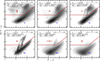 |
Fig. 1. Galaxies identified as either star-forming or quiescent based on their NUV − r and r − J rest-frame colours at z ≤ 3. Rest-frame colours are measured using LePHARE following Ilbert et al. (2005). Representative uncertainties associated with the rest-frame colours of the star-forming (blue) and quiescent (maroon) subsamples are plotted. At z > 1.5, the Balmer break is redshifted between two observed bands (HSC z and IRAC [3.6 μm]), and so the inferred rest-frame colours become increasingly model-dependent. Shading corresponds to logarithmic density. |
The decrease in the number of quiescent galaxies with increasing redshift apparent from Fig. 1 is a consequence of both well-understood aspects of galaxy evolution (Ilbert et al. 2013) and observational effects. Considering the latter, the selection function described in Sect 3.1 determines the ability to detect quiescent galaxies from the DAWN survey PL images. After redshift z ∼ 1.6, the Balmer breaks drops out of the HSC z band, and consequently galaxies above z ∼ 1.6 are detected on the basis of increasingly blue rest-frame light.
These results broadly agree with W23. Namely, the fraction of massive quiescent galaxies is similar, up to z∼ 2–3. However, the DAWN PL catalogue is optically selected leading to a dearth of detected quiescent galaxies at z > 3. While expected, it limits the exploration of quiescent (and generally red) objects to z < 3. Consequently, the total sample at z > 3 contains only blue, star-forming galaxies without significant dust attenuation. Future work incorporating Euclid’s NIR bands will complete this picture.
3.3. Galaxy stellar mass limit
Measuring the galaxy SMF requires identifying the minimum stellar mass at each redshift above which galaxies are detected. Pozzetti et al. (2010) presented a method that is often used (Ilbert et al. 2010, 2013; Muzzin et al. 2013; Tomczak et al. 2017; Davidzon et al. 2017; Stefanon et al. 2021; Weaver et al. 2023a) to empirically measure the stellar mass limit of a survey based on the measured stellar masses of detected galaxies and the limiting flux of the survey. The method consists of converting the flux limit of a given survey to a stellar mass limit by first inferring a mass-to-light ratio, applying a transformation to the measured stellar masses given the difference between their measured flux and the limiting flux, and using the rescaled stellar masses to describe the completeness limit. Here, the implementation of the Pozzetti et al. (2010) method by W23 is followed, considering only the 99% best-fit objects by χ2 from Sect. 3.1. Subsequently, the galaxies with the 30% lowest stellar masses are selected as being representative of those near to the stellar mass limit. The stellar masses of this subsample are rescaled following Pozzetti et al. (2010):
 (2)
(2)
where mz is the apparent magnitude in the HSC z band and 26.9 is the approximate 3σ limiting magnitude in the combined HSC r + i + z images (Euclid Collaboration: Zalesky et al. 2025). Galaxies below log10(ℳ/M⊙) < 8 are not expected to be detectable and are therefore not considered in calculating the mass completeness. The galaxies with rescaled stellar masses are binned according to their redshift, with a spacing of Δz = 0.2. In a further effort to be conservative, the 95th percentile of the rescaled masses (ℳresc) is used to identify the stellar mass limit in each bin, in contrast to the 90th percentile used by W23. Finally, an analytical function is fit to the binned mass completeness limits of the form ℳz = A(1 + z)B. However, unlike W23, who used a flexible expansion in (1 + z), this choice is simpler, provides a better fit per degree of freedom, and is consistent with D17, which shares similar NIR imaging depth.
The stellar mass limit is computed for the total sample, star-forming sample, and quiescent sample independently according to the method above. The results are as follows:
 (3)
(3)
 (4)
(4)
 (5)
(5)
As can be inferred from Eqs. (3, 4), the stellar mass limit of star-forming galaxies is similar to that of the total sample, differing only at the highest and lowest redshifts. Meanwhile, the stellar mass limit of quiescent galaxies is a significantly stronger function of redshift. The results are depicted in Fig. 2 over a two-dimensional histogram of redshift and stellar mass, ℳ. Because there are so few quiescent galaxies detected at z > 2, the low-redshift galaxies have the dominant weight in the fit of the ℳz = A(1 + z)B function. In practice, quiescent galaxies below the total stellar mass limit (left panel of Fig. 2) are not considered, thereby ensuring consistency across the samples. The stellar mass limits of D17 and W23 are also shown. By comparison, the stellar mass limits of DAWN PL, computed according to the HSC z band, are shallower. This is not surprising, given that both D17 and W23 utilise a detection image incorporating NIR data. Consequently, DAWN PL is not ideal for describing the galaxy SMF to the lowest stellar masses. Instead, deeper programmes (e.g. Furtak et al. 2021) are preferable to study the low-mass end. Nonetheless, the stellar mass limit reached by DAWN PL is sufficient to study massive galaxies ℳ > 1010 M⊙ at all redshifts.
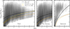 |
Fig. 2. Galaxy stellar mass distribution as a function of redshift. The limiting stellar mass of the total (left), star-forming (middle), and quiescent (right) samples are determined as a function of redshift following Pozzetti et al. (2010) and are shown by the solid black curves. Two estimates are computed based on the limiting magnitude of HSC z (solid) and the IRAC [3.6 μm] limiting magnitude (dotted), respectively. The more conservative estimate using HSC z is used in the remainder of this work and are presented as Eqs. (3)–(5) for the total, star-forming, and quiescent samples. For comparison, the stellar mass limits of D17 and W23 are also shown. Shading corresponds to logarithmic density. |
It may be reasonable to use the [3.6 μm] or [4.5 μm] apparent magnitude and the corresponding limiting magnitude in the rescaling equation (Eq. 2) to determine the stellar mass limits of DAWN PL. Recall that a 3σ detection in the Spitzer/IRAC [3.6 μm] and [4.5 μm] bands is required (Sect. 3.1) for a source to be considered. The result of using [3.6 μm] to derive the limiting stellar mass limits is included in Fig. 2. This calculation provides stellar mass limits that are notably deeper than those obtained when using HSC z, and similar to that obtained by D17. However, to avoid any pitfalls associated with extrapolating from the selection function in the HSC r + i + z bands to a stellar mass limit derived with [3.6 μm], the conservative option of the HSC z-derived stellar mass limits is used.
It should be understood that the method of Pozzetti et al. (2010) provides an estimate of the limiting stellar mass above which a galaxy is detected given the selection function. Consequently, the stellar mass limits quantified by Eqs. (3)–(5) may be overly optimistic for galaxies that are difficult to detect, given the selection function defined by the HSC r + i + z bands. Such galaxies primarily include intrinsically red objects, such as significantly dust-attenuated star-forming galaxies and quiescent systems at z > 1.5.
For now, it is assumed that the selection function and the significant depth of the detection image is sufficient to identify a substantial fraction of galaxies above the stellar mass limit to z ∼ 6. To support this hypothesis, consider that the 3σ limiting magnitude in the UltraVISTA (McCracken et al. 2012) NIR Ks band of the COSMOS2020 catalogue is ∼25 (and shallower for the COSMOS2015 catalogue used by D17, between 24 and 24.7 mag depending on the area; see Laigle et al. 2016). Selecting galaxies brighter than Ks ≤ 25 that also satisfy the selection criteria for the mass function specified by W23 indicates that galaxies from 3 < z ≤ 6 span a range in colour z − Ks where the 90th percentile is approximately 2.5 mag at z ∼ 3, dropping to ∼2 mag at z ∼ 4, and continuing to fall < 1 by z ∼ 6. Accordingly, a significant majority of red galaxies according to z − Ks should be detected by the combined depth of the HSC r + i + z image that reaches at least 26.9 mag in the HSC z. Further, the galaxy SMFs presented in Sect. 5 appear to support this hypothesis, at least to a similar completeness achieved by D17 to z ∼ 5. It is possible that the stellar mass limit is underestimated in the highest-redshift bins considered in this work at z > 4.5. However, the significant volume of DAWN PL provides a unique opportunity to characterise the abundance of massive galaxies at this epoch, and so the redshift bins above z > 4.5 are included, despite the possibility of incompleteness.
3.4. Uncertainty and bias estimation
The total uncertainty of the observed galaxy SMF has at least three general components. As for any statistical characterisation that involves counting N samples drawn from a parent population, the galaxy SMF is affected by Poisson uncertainty (σN; Sect. 3.4.1). An additional source of uncertainty that must be accounted for is the cosmological fluctuation of galaxy properties (in particular stellar mass) on the physical scales observed by the survey, an effect commonly referred to as ‘cosmic variance’ (σCV; Sect. 3.4.2). Lastly, the galaxy SMF is impacted by the choices and assumptions made during the SED modelling insofar that they impact the photometric redshifts and galaxy stellar masses (σSED; Sect. 3.4.3). The total uncertainty is the quadrature added sum of the three main components, i.e.  .
.
3.4.1. Poisson
Poisson uncertainty reflects the statistical noise from finite sampling and is estimated for each ℳ bin as  . We computed this separately for total, star-forming, and quiescent populations. Thanks to the ∼10× larger area of DAWN PL compared to COSMOS, the Poisson uncertainty was reduced by a factor of ∼3 relative to W23, enabling robust constraints at ℳ ≳ 1011 M⊙ across all redshifts. These uncertainties are shown in the left panel of Fig. 3.
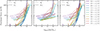 |
Fig. 3. Three components of the total uncertainty of the number density in each ℳ bin, σΦ: the Poisson uncertainty (σN; left), cosmic variance (σCV; middle), and uncertainty arising from SED fitting (σSED; right). The total uncertainty, shown by the dashed lines in each panel, is the quadrature sum of the three components, shown by the solid lines in each panel. |
For a given volume, the Poisson upper limit may also be determined by considering the Nbin = 0 case. Following Gehrels (1986), the 1σ upper limit for an Nbin = 0 event in a volume V is 1.841/V, while the 3σ upper limit is 6.61/V (see also Ebeling 2004). The 1σ upper limit is illustrated in many of the figures shown in Sect. 5 by a downward pointing arrow.
3.4.2. Cosmic variance
In one aspect, the Poisson uncertainty described above (Sect. 3.4.1) represents the minimum error on the number of galaxies expected in a given bin. However, the Poisson uncertainty assumes that galaxies properties, including the stellar masses and their spatial distributions, are independent. In reality, galaxy properties are known to be spatially correlated (Kauffmann et al. 2004; Wu & Kragh Jespersen 2023; Wu et al. 2024), and moreover, environments differ on cosmological scales, in part due to large-scale fluctuations in the cosmic density field that have grown since the Big Bang (Springel et al. 2005). From observations, it has been shown the galaxies cluster more strongly than their dark matter halos, and from simulations, it is predicted that such galaxy ‘bias’ increases across redshift (Moster et al. 2010). Importantly, more massive systems are more biased than their lower-mass counterparts. Since it is impossible to know a priori where a given field is sitting in the global large-scale structure fluctuation, and smaller areas are naturally affected by both long- and short-wavelength fluctuations, galaxy surveys with small areas are more strongly affected by field-to-field variance, referred to as ‘cosmic variance’, σCV, than larger surveys of equal depth. See Moster et al. (2010, 2011) for a review.
The estimation of cosmic variance used in this work differs from W23, which relied on cosmic variance calculations provided by Moster et al. (2011) that were extrapolated by Steinhardt et al. (2021) to higher redshifts and greater stellar masses. Instead, the method of Jespersen et al. (2025) is followed, wherein the authors demonstrated a method for more robustly deriving cosmic variance estimates for massive galaxies at a range of redshifts using the UniverseMachine simulations (Behroozi et al. 2019). A brief summary follows, although the reader is referred to Jespersen et al. (2025) for details. Each survey field of DAWN PL, i.e. EDF-N and EDF-F, is treated independently, as they are highly separated and thus not in causal contact. Number counts of galaxies are sampled from a survey volume corresponding to the areas of the two fields, 8.42 deg2 for EDF-N and 1.71 deg2 for EDF-F. In addition, the same redshift and mass bins defined by this work (see Table 1 and Sect. 5) are imposed on the selection. The variation in the number counts that is in excess of the Poisson uncertainty and due to clustering of galaxies is modelled by a power law in stellar mass with a redshift-dependent normalisation and slope. The calibration of the final model of cosmic variance also includes error terms identified by Jespersen et al. (2025), which correct the cosmic variance estimates for the impact of the skew of the underlying distribution of number counts in single bins3. The total cosmic variance σCV, tot across the combination of EDF-N and EDF-F, is given by
![Mathematical equation: $$ \begin{aligned} \sigma _{\mathrm{CV,\ TOT} } = [(\sigma _{\mathrm{CV,\ N} })^{-2} + (\sigma _{\mathrm{CV,\ F} })^{-2}]^{-1/2}, \end{aligned} $$](/articles/aa/full_html/2026/04/aa55728-25/aa55728-25-eq10.gif) (6)
(6)
where σCV, N is the cosmic variance corresponding to the volume of EDF-N and σCV, F is the cosmic variance corresponding to the volume of EDF-F.
The σCV estimates for the combination of EDF-N is presented in the centre panel of Fig. 3. Given the significant volume of DAWN PL and the improvement of the method of Jespersen et al. (2025) over Moster et al. (2011), the impact due to cosmic variance is significantly smaller in comparison to D17 and W23. For example, the uncertainty due to cosmic variance is at least a factor of 5 times greater in W23 for galaxies of ℳ ∼ 1010.5 M⊙ at z ∼ 5.
3.4.3. SED fitting
As described above, galaxy properties are measured using LePHARE closely following the procedure of W23 (as well as Ilbert et al. 2013 and D17, though to a lesser degree). SED modelling assumptions (e.g. parametric star-formation histories) are the same as detailed in Ilbert et al. (2013). EC-Z25 validated the photo-z measurements for DAWN PL by comparing with 3300 high-quality spectroscopic redshifts matched from GOODS-S (Garilli et al. 2021; Kodra et al. 2023) that sample 0 < z ≤ 5.5 (see Figs. 8 and 9 of EC-Z25). In addition, the authors modified the photometric errors of COSMOS2020 catalogue to match those of the DAWN survey PL catalogue and used LePHARE to re-measure photo-z and ℳ utilising only the filters available to DAWN PL. The results demonstrated that more than 80% of all galaxies had consistent redshifts and stellar masses. The majority of the those that are not consistent are too faint to satisfy the selection criteria used in the present work (see Fig. 11, and Appendix C of EC-Z25). As such, the photo-z and ℳ measurements provided by DAWN PL are believed to be robust, especially in view of the requirements applied in Sect. 3.1. Nonetheless, the impact of the uncertainties associated with modelling the SEDs must be accounted for and propagated through to the resulting uncertainty on the galaxy SMF.
Under the configuration applied across Ilbert et al. (2013), D17, and W23, as well as here, photo-z and ℳ estimates are obtained separately, utilising a different template set for each calculation (see Weaver et al. 2022 and EC-Z25 for details). More specifically, the physical properties of galaxies are inferred assuming a fixed redshift, z ≡ zphot. At the time of writing, LePHARE does not support allowing the redshift to vary using one template set while measuring physical properties using another template set. Consequently, the uncertainties on ℳ provided in the DAWN survey PL catalogues do not include the covariance between photo-z and ℳ. Facing a similar situation, W23 relied on the extreme photo-z precision achieved by the COSMOS2020 catalogue and suggested that their σSED measurements should be considered lower limits. By contrast, D17 performed a Markov chain Monte Carlo (MCMC) simulation of their entire catalogue by varying the photometric measurements within their uncertainties measuring a new photo-z and ℳ one thousand times. Similar approaches have been used elsewhere (G15). However, D17 used a sample of galaxies that is more than an order of magnitude smaller than the DAWN PL sample, and applying their approach to DAWN PL is not computationally tractable at present4.
A zeroth-order correction to the impact of the stellar mass uncertainties on the measured galaxy SMF, addressing the covariance between redshift and mass, is obtained as follows. Recall that galaxies are required to have 68% of their redshift probability distribution contained within the interval zphot ± 0.5. In addition, EC-Z25 demonstrated with a high-quality sample of 3300 spectroscopic redshifts matched from GOODS-S (Garilli et al. 2021; Kodra et al. 2023) that 68% of all galaxies with spectroscopic redshifts had photo-z measurements within 1σ of their spectroscopic value. As such, photo-z probability distributions for galaxies used here are narrow and appear well calibrated. Therefore, instead of determining new redshifts for each galaxy by re-running LePHARE, 1000 redshifts for each galaxy are drawn from the respective redshift PDFs. To zeroth order, the stellar mass inferred for a galaxy at z1 + δz compared to its inferred stellar mass at redshift z1 will differ by a re-scaling proportional to δz, similar to their absolute magnitudes. This is because at small δz, the inferred galaxy type will not change and therefore the inferred mass-to-light ratio will be approximately constant. Assuming the k-correction is small, the difference in absolute magnitudes (dM) between two galaxies with the same apparent magnitude but at redshifts z1 and z2 = z1 + δz is
 (7)
(7)
where dL(z) is the luminosity distance to a galaxy at redshift z.
At each newly drawn redshift, the galaxy stellar mass, ℳ, is scaled according to Eq. (7). It is acknowledged that a range of mass-to-light ratios are allowed for a particular galaxy given its photometric uncertainties, and so an additional perturbation to the rescaling factor is applied in proportion to the relative flux errors. Lastly, a final perturbation that is proportional to the difference in mass that would be obtained from a random draw from the ℳ probability distribution function (PDF) from LePHARE is applied. Note that because δz is small, the original stellar mass PDF should still be approximately representative, given that it is largely driven by photometric uncertainties (Ilbert et al. 2013; Davidzon et al. 2017; Weaver et al. 2023a). However, it too must be scaled according to Eq. (7) to account for the newly assigned redshift. The final result of this exercise is 1000 independent realisations of galaxy photo-z and ℳ estimations, where each ℳ value has been adjusted to the newly assumed redshift while accounting for a variety of possible mass-to-light ratios and further scattered due to shape of the PDF of stellar mass. This includes 2.3 trillion total measurements.
The simulated photo-z and ℳ measurements are used to construct 1000 realisations of the galaxy SMF, using the same redshift and stellar mass bins as the primary analysis (see Sect. 5). The uncertainty due to SED fitting, σSED, is then quantified for each redshift bin by measuring the 1σ variation in the number density at every ℳ bin relative to the median number density. The result is shown in the right panel of Fig. 3. The scale of σSED follows a similar trend compared to σN, reflecting the abundance of low-mass galaxies that have a number density that does not change appreciably due to SED fitting. By contrast, massive galaxies with ℳ > 1011.5 M⊙ have uncertainties in their abundance of order unity.
Although effort has been taken to account for the covariance between stellar mass and redshift, the estimated σSED are expected to be valid in the regime of small variations in the assumed redshift. The analysis has not accounted for catastrophic outliers in redshifts, or the choice of templates used by LePHARE, for example, given that systematic errors are not easily combined with random errors. Improving the computational time required to run current SED-fitting codes is imperative for future datasets even larger than DAWN PL.
3.4.4. Validation
Several requirements have been established above in order to obtain a sample of galaxies with only the most robust estimates of their properties. With trustworthy estimates of galaxy properties in place, it is possible to characterise the evolution of the galaxy SMF across cosmic time. Interpreting the observed galaxy SMF is strengthened by an understanding of the success of these efforts, or lack thereof, and any resulting systematics. A stronger understanding of these systematics is also vital to infer the intrinsic galaxy SMF with confidence (Sect. 5.4). To this end, Appendix B provides a detailed discussion of a series of validation tests that have been performed on the DAWN PL data. The validation tests and their findings are summarised below.
-
Re-fitting COSMOS2020 with only DAWN PL filters: COSMOS2020 (Weaver et al. 2022) includes photometry in all of the filters used by DAWN PL, but with deeper imaging. EC-Z25 demonstrated a test wherein photo-zs and stellar masses were recomputed for all of COSMOS2020, utilising only the filters available to DAWN PL and with flux uncertainties scaled to match DAWN PL. Galaxies are further selected from a detection imaging comprising the same noise properties as that of DAWN PL. Using measurements entirely from the re-fitting, the COSMOS2020 galaxy SMF is measured and compared with W23, finding excellent agreement with one primary exception. Galaxies at z ∼ 1.1–1.5 are found to have degenerate template solutions, which given the decreasing sample size with redshift, leads to an underestimation of low-mass galaxies at these redshifts and an overestimation of massive galaxies at higher redshifts 1.5 < z ≤ 2.5 (see Appendix B.1 and Sect. 5.4). There is no significant bias detected above z = 2.5 except for what is predicted by the difference in selection functions. The agreement between W23 with the SMF derived using only the DAWN PL filters lends confidence to the results presented here.
-
Validating galaxy properties through machine learning: Following Chartab et al. (2023), a random forest regressor model is trained on COSMOS2020 restricted to the DAWN PL bands to predict galaxy properties from the DAWN PL photometry. The performance of both the resulting photo-z and stellar mass estimates are consistent with those obtained from SED fitting using LePHARE with mild improvement from test galaxies in COSMOS2020. The galaxy SMF may be measured using the galaxy properties predicted from the DAWN PL catalogues, and the result improves the characterisation of galaxies at 1.1 < z ≤ 2.5. However, the conservative nature of the random forest regressor prohibits predictions of galaxy properties outside its training data, and therefore its ability to accurately determine the properties of galaxies with extreme values may be limited. Galaxies with properties that disagree between those obtained from the random forest and from LePHARE likely include discoveries that would be missed by a random forest.
4. Galaxy SMF formalism
Below, the mathematical formalisms for inferring the intrinsic galaxy SMF used in this work are described.
4.1. Consideration of volume
Compared to their fainter counterparts, bright galaxies are rarer at every redshift. However, in a flux-limited survey, intrinsically faint galaxies are comparatively more difficult to observe at every redshift and so can appear underrepresented. A correction to this ‘Malmquist’ bias (Malmquist 1922, 1925) was presented by Schmidt (1968) and is now commonly employed in galaxy demographic studies, including those targeting the galaxy luminosity function and the galaxy SMF due to its simplicity. This correction is referred to as the 1/Vmax correction and prescribes that every galaxy is weighted by the maximum volume (i.e. Vmax) in which it could be observed. In this work, galaxies are first binned according to their redshift and binned again according to their ℳ. Following Schmidt (1968), every galaxy (i) is weighted by
![Mathematical equation: $$ \begin{aligned} V_{\mathrm{max} , i}=\frac{4 \pi }{3} \frac{\Omega _{\mathrm{survey} }}{\Omega _{\mathrm{sky} }}\left[d^3_{\rm c}\left(z_{\mathrm{high},i}\right)-d^3_{\rm c}\left(z_{\mathrm{low},i}\right)\right], \end{aligned} $$](/articles/aa/full_html/2026/04/aa55728-25/aa55728-25-eq12.gif) (8)
(8)
where Ωsurvey is the solid angle spanned by the survey (in square degrees, 10.12 deg2), Ωsky is the solid angle of the entire sky, i.e. 41 253 deg2, and dc is the co-moving distance. The maximum volume a within which a galaxy could be observed is bounded on the low end (zlow) by the lower edge of the redshift bin and on the high end (zhigh) by the maximum redshift at which the galaxy could be observed without falling below the detection limit. For bright galaxies, the high end is effectively the upper edge of the redshift bin. The redshift bins used throughout match those used by D17 and W23 and are provided in Table 1.
Hereafter, number densities in each redshift bin and mass show are reported after having applied the Vmax corrections. It is noted that additional methods for characterising the SMF are explored in the literature (see e.g. Weigel et al. 2016 and citations therein). However, discrepancies in comparing the results do not appear strong enough to warrant departing from the 1/Vmax method (D17).
4.2. The Schechter function
The number density of galaxies as a function of stellar mass (and luminosity) are frequently reported as following an analytical characterisation first introduced by Schechter (1976) and since known as the ‘Schechter’ function. The Schechter function can be written to describe the specific number density of galaxies as a function of stellar mass, Φ(ℳ), by
 (9)
(9)
Conceptually, the Schechter function describes the number density as a power law with slope α for galaxies below a characteristic mass, ℳ★ followed by an exponential decline. Both components are scaled by an overall normalisation Φ★. The characteristic mass ℳ★ defines the point at which the Schechter function ‘turns over’ and is sometimes referred to as the ‘knee’ of the galaxy SMF. The evolution of the Schechter parameters across cosmic time is a topic of debate in the literature.
Although the Schechter function is predominantly used as an empirical description, Peng et al. (2010) presented a theoretical framework that gives rise to a Schechter function in the observed number counts. Further, Peng et al. (2010) predicted and demonstrated that, depending on their types and environments, the distribution of galaxies as a function of their stellar mass can be described by a ‘double’ Schechter function:
![Mathematical equation: $$ \begin{aligned} \Phi (\mathcal{M} )\; \mathrm{d} \mathcal{M} =\left[\Phi _1^{\star }\left(\frac{\mathcal{M} }{\mathcal{M} ^{\star }}\right)^{\alpha _1}+\Phi _2^{\star }\left(\frac{\mathcal{M} }{\mathcal{M} ^{\star }}\right)^{\alpha _2}\right] \exp \left(-\frac{\mathcal{M} }{\mathcal{M} ^{\star }}\right) \frac{\mathrm{d} \mathcal{M} }{\mathcal{M} ^{\star }}. \end{aligned} $$](/articles/aa/full_html/2026/04/aa55728-25/aa55728-25-eq14.gif) (10)
(10)
The double-Schechter function adds a second power-law component with its own normalisation (Φ2★) and slope (α2), though each power-law term is joined by the same characteristic mass ℳ★ above which there is an exponential decline.
The physical meaning and the validity of the Schechter function (and the double-Schechter function), insofar that it describes the observed galaxy SMF in this work, is discussed further in Sects. 5 and 6. Indeed, additional parametric descriptions have been suggested in the literature, for example, D17 postulated that the SMF of galaxies at z ∼ 5 is a power law.
4.3. Eddington bias
Any observed distribution function that is both non-linear and has a non-zero second derivative of the observed variable will differ from the true underlying distribution by the so-called ‘Eddington’ bias (Eddington 1913, 1940; see also Teerikorpi 2004). The galaxy SMF is a distribution function of this type (as are apparent magnitude distributions and luminosity functions). The effect is most prominent for the most massive systems due to their rarity. For example, under the Schechter formalism, the exponential overturn after ℳ★ poses a strong second derivative. The consequence is that the observed number density of massive galaxies is higher than the true underlying number density due to less massive galaxies, which are far more abundant, being randomly scattered into higher-mass bins because of their uncertainty in stellar mass. By contrast, massive galaxies being scattered into low-mass bins has a much less significant effect because of their relative abundance, providing fewer instances to scatter and causing a smaller relative change to the number of galaxies in the bin.
Given a parametric representation of the true underlying galaxy SMF, such as the Schechter function or the double-Schechter function, the observed distribution can be described by a convolution of the parametric function with a kernel, 𝒟(ℳ), that characterises the uncertainty in stellar mass. The intrinsic galaxy SMF may then be inferred via deconvolution. In this work, the same kernel utilised by Ilbert et al. (2013), D17, and W23 is used to characterise the stellar mass uncertainties:
 (11)
(11)
The kernel includes a Gaussian component of standard deviation σEdd that conveys the scatter in the stellar mass primarily due to photometric uncertainties. The Gaussian component is multiplied by a Lorentzian component that broadens the distribution to further account for the more drastic changes in stellar mass that result from uncertainty in the redshift. The Lorentzian component is characterised by the parameter τEdd, which is redshift-dependent, i.e. τEdd = τc(1 + z), reflecting the fact that generally photometric redshifts are less certain with increasing z.
The exact values of τEdd and τc are determined by fitting the marginalised probability distributions of mass obtained from Sect. 3.4.3, following Ilbert et al. (2013) and D17. The distributions are well described by Eq. (11) but larger values for σEdd and τc are obtained compared to D17, i.e. σEdd = 0.6 and τc = 0.05 compared to σEdd = 0.35 and τc = 0.04, respectively. The increased uncertainty relative to D17 is likely due to the lower number of photometric filters considered in the present work, although the values are very similar to those obtained by Ilbert et al. (2013).
It is noted that the treatment of the Eddington bias may play a significant role in driving discrepancy between different measurements of the galaxy SMF in the literature (Grazian et al. 2015; Davidzon et al. 2017). Adams et al. (2021) explored the impact of several representations for the convolution kernel, including a Gaussian kernel, the kernel of Eq. (11), and an empirically constructed kernel based on the posterior distribution resulting from varying galaxy redshifts and stellar masses. The authors found that utilising the kernel of Eq. (11) obtained results essentially consistent with the empirically constructed kernel but differing from the results using the Gaussian kernel. Further consideration of the impact on the choice of convolution kernel is discussed in Sect. 6.
5. Results
The total observed galaxy SMF is presented, followed by the star-forming and quiescent components. The intrinsic galaxy SMF is obtained by modelling the observed SMF according to the formalisms defined above. Finally, the cosmic stellar mass density (SMD) is calculated by integrating the intrinsic SMF. Throughout, the galaxy SMF is measured according to the redshift bins defined in Table 1 and using ℳ bins of width 0.25 dex.
5.1. Total stellar mass function
The total galaxy SMF from 0.2 < z ≤ 6.5 is shown in Fig. 4. The evolution of the total galaxy SMF is often discussed in the context of galaxies below and above the characteristic mass ℳ★, delineating ‘low-mass’ and ‘massive’ galaxies. Following the dark matter HMF (e.g. Tinker et al. 2008), low-mass galaxies overwhelmingly dominate the galaxy SMF at all redshifts but especially at high z where large-scale structure has yet to form. Beyond a general description, the low-mass end of the galaxy SMF is mostly inaccessible through DAWN PL due to the stellar mass limit being greater than ℳ > 109 M⊙ at all redshifts and increasing to ℳ > 1010 M⊙ by z ∼ 3. However, the substantial volume of DAWN PL enables a statistically significant characterisation of the abundance of massive galaxies above ℳ > 1010.5 M⊙ across the entire range of 0.2 < z ≤ 6.5.
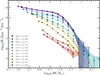 |
Fig. 4. Evolution of the observed galaxy SMF of the total sample across 0.2 < z ≤ 6.5. The ℳ bins are uniform except for the first bin, which is extended to the respective stellar mass limit. The ℳ bins below the stellar mass limit (Eq. 3) are not shown. Uncertainties are indicated by the solid error bars and shaded regions. |
Before inferring the intrinsic galaxy SMF, a few conclusions can already be drawn. First, the early Universe was characterised by a period of rapid star formation. Several previous observations have shown that although star-formation rates peak at z ∼ 2, specific star-formation rates were significantly higher in the early Universe (Behroozi et al. 2013; Madau & Dickinson 2014). The age of the Universe at redshift z ∼ 6 corresponds to 0.92 Gyr after the Big Bang under the assumed cosmology. From z ∼ 6 to z ∼ 3.25, a time span of 1 Gyr, the abundance of galaxies with mass ℳ ∼ 1010.5 M⊙ increased by a factor of at least 100. By contrast, the abundance of galaxies of similar mass grew only by a factor of 10 between z ∼ 3.25, and z ∼ 0.35 despite spanning a significantly longer period of time (7.7 Gyr). This is essentially an extension of the ‘down-sizing’ effect (Cowie et al. 1996). Additional features of the total galaxy SMF are better understood in view of a comparison with previous results from the literature (Sect. 5.3) and from an analysis of the intrinsic, rather than observed, galaxy SMF (Sect. 5.4).
It is emphasised that for now, only the observed galaxy SMF is presented, while the intrinsic galaxy SMF is presented in Sect. 5.4. As such, seemingly unphysical features, such as higher-redshift bins containing a greater abundance of massive galaxies compared to lower-redshift bins, are almost certainly due to Eddington bias that has yet to be removed. The discussion in Sect. 6.4 and Appendix B further discuss the likely contamination of galaxies from the redshift bin 1.1 < z ≤ 1.5 to the next two higher-redshift bins. As such, the galaxy SMF within this redshift interval should be considered with caution, as is discussed further below.
5.2. Star-forming and quiescent stellar mass functions
The star-forming and quiescent components of the total galaxy SMF are separated using the NUVrJ criteria described in Sect. 3.2. Total uncertainties for each component are computed following Sect. 3.4 for each galaxy type and redshift interval. Given the DAWN PL selection function, only the most massive (ℳ > 1011 M⊙) and brightest quiescent galaxies are detectable at z > 2. Consequently, the shape of the quiescent galaxy SMF is not well constrained at these redshifts. For example, at 2 < z ≤ 2.5, only 732 quiescent galaxy candidates above the mass completeness limit spanning five ℳ bins are found over the entire DAWN PL area. At 2.5 < z ≤ 3, the number drops by over an order of magnitude to 57 in three ℳ bins. Above z > 3, no quiescent galaxies are detected that satisfy the necessary criteria.
5.3. Comparison with the literature
The evolution of the total galaxy SMF is compared with measurements from D17 and W23 in Fig. 5 across 0.2 < z ≤ 3.5. Each work uses the same redshift binning, beginning at 0.2 < z ≤ 0.5, and the same ℳ binning. In Fig. 5, the coloured arrow indicates the 1σ Poisson upper limit for zero detections given the volume of DAWN PL, while the grey arrow indicates the same for the volume of W23 (about a factor of 2 smaller than D17). Although galaxies detected at values of Φ lower than these limits may be real, they do not meaningfully constrain the SMF.
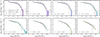 |
Fig. 5. Observed total galaxy SMF of DAWN PL (coloured points) and uncertainties (1σ, shaded) compared with two measurements from COSMOS, D17 and W23, through to 3 < z ≤ 3.5. ℳ bins below the stellar mass limit (Eq. 3) are not shown. The volume limit according to the N = 0 Poisson uncertainty is shown by the downward pointing coloured arrow for DAWN PL and in grey for W23. |
Figure 5 confirms that at least through z ≤ 3.5 the deep optical imaging of DAWN PL provides a sample of galaxies that is almost entirely consistent with a shallower NIR selection, such as the selection of D17, as suggested in Sect. 3.1. In addition, the overall shape and normalisation of the total SMF is in agreement with both D17 and W23. However, as noted in Sect. 3.2, the selection function of DAWN PL precludes the detection of a sizeable fraction of intrinsically red objects above z = 1.5, which may explain the deviation of the PL SMF at 2 < z ≤ 2.5 in the vicinity of the knee (ℳ ∼ 1010.9 M⊙) compared to both D17 and W23.
A more significant point of disagreement is within the redshift interval 1.1 < z ≤ 2.5, which has been briefly discussed in Sect. 3.4.4 and is treated more extensively in Appendix B. Beginning at 1.1 < z ≤ 1.5 up until z ∼ 2, there are too few galaxies per unit volume found by DAWN PL within the ℳ range that should be complete. The dearth of galaxies at 0.8 < z ≤ 2.0 may be related to the relative excess of ℳ ≫ ℳ* galaxies at z > 2.0. Without a strong observed constraint on the Balmer break, the high-redshift solutions during SED fitting outnumber low-redshift solutions, causing a systematic trend towards higher redshifts and correspondingly higher masses (due to the redshift-mass covariance). As demonstrated in Appendix B, this systematic bias can be remedied through machine learning techniques, suggesting that the bias is caused by a degeneracy in the LePHARE templates rather than the DAWN PL photometry. At this time, it is not clear how to best apply a correction that does not cause an inconsistency in other redshift bins. Ultimately, this is a strong example of Eddington bias at play (due to the uncertainty in stellar mass driven by the covariance with redshift), and as such, the biased redshift bins of 1.1 < z ≤ 2.5 provides a test-case to assess whether the treatment of Eddington bias (Sect. 4.3) is sufficient. The subject is picked up again in Sect. 5.4.
As previously discussed, the photo-z bias is not expected at z > 2.5 where the Lyman break is directly constrained (see Appendix B). At 2.5 < z ≤ 3.5, the abundance of the most massive systems observed in COSMOS by both D17 and W23 is confirmed with significantly improved precision due to the improvement in Poisson uncertainty and cosmic variance by DAWN PL. Within this redshift range, DAWN PL also finds a handful of galaxies of greater mass than have been observed in COSMOS. Most of these galaxies are within the 1σ volume limit, consistent with no detection. At 3 < z ≤ 3.5, a significant number of galaxies are found at masses greater than were observed by D17. W23 report an even more significant excess of galaxies compared to D17 at 3 < z ≤ 3.5, most noticeable above ℳ > 1011 M⊙. However, the total galaxy SMF of DAWN PL is consistent with both works within their reported 1σ limits. By inspecting the COSMOS2020 catalogue, the galaxies at 3 < z ≤ 3.5 missed by DAWN PL appear intrinsically red and optically faint (e.g. with HSC i ≫ 26), perhaps indicative of dusty star forming systems that are mostly undetected without NIR imaging.
Beginning at 3.5 < z ≤ 4.5, the total galaxy SMF is further compared with results from Grazian et al. (2015, hereafter G15) and Weibel et al. (2024, hereafter W24) in Fig. 6. However, it is cautioned that both cover areas that are a factor of 70–100 smaller than DAWN PL (369 arcmin2 and 500 arcmin2, respectively), and a significant increase in cosmic variance should be expected. At 3.5 < z ≤ 4.5, DAWN PL continues to be consistent with D17 while also finding galaxies at greater masses, further confirming the utility of deep optical imaging to detect significant samples of galaxies at least to z ∼ 4. The comparison further shows an agreement between DAWN PL with G15 that may at first be surprising given the difference in selection functions. G15 detects galaxies using the WFC3 H160 band with a depth that significantly exceeds that of D17, yet their number densities are consistent with each other as well as with DAWN PL. Meanwhile, both DAWN PL and D17 present number densities of massive galaxies (i.e. with masses ℳ > 1011 M⊙) that are slightly lower than the measurements of both W23 and W24. W24 explains that their excess at z ∼ 4 is largely driven by very red galaxies that are missed by HST and therefore should also be missed by ground-based optical surveys. However, the deep Ks imaging utilised by W23, deeper than was available to D17 by ∼0.5 mag, coupled with their significantly increased volume in comparison to W24, appears to confirm a similar abundance.
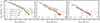 |
Fig. 6. Same as Fig. 5 but at z > 3.5 and also showing measurements from G15 with HST (grey circles) and W24 with JWST (grey squares). |
The deep optical imaging of DAWN PL is sufficient to obtain a significant sample of galaxies at 4.5 < z ≤ 5.5. Above ℳ > 1011 M⊙, the number density is in agreement with D17 within the reported 1σ uncertainties and consistent with the abundance of W23 within their 2σ uncertainties (not shown; see W23, Fig. 6). Further comparison with G15 and W24, both of which make use of deep space-based observations, shows similar agreement within the range of masses that overlap. However, the literature ultimately points towards an incompleteness in DAWN PL of galaxies with masses 1010 < ℳ/M⊙ < 1011. The stellar mass limit of DAWN PL is compared to W23 and explored in greater detail in Appendix B in an analysis that suggests the completeness at 1010 < ℳ/M⊙ < 1011 is between 40–60% in DAWN PL. Notably, W23 finds a sample of galaxies with masses greater than those observed by G15 and D17. DAWN PL provides a sample of galaxies at 4.5 < z ≤ 5.5 that are equally massive and have a number density that is consistent within 1σ, although those of DAWN PL are more numerous and therefore more statistically significant assuming the uncertainties are well measured (Sect. 3.4). In addition, there are 13 galaxies in DAWN PL with masses exceeding the most massive one found in W23. Interestingly, with the assistance of deep JWST imaging, W24 finds two such galaxies with ℳ > 1011.6 M⊙, but given their limited area, their number density is consistent within the Poisson 1σ upper limit of zero detections.
Despite the inclusion of NIR imaging, D17 was not able to find a significant sample of galaxies at 5.5 < z ≤ 6.5. By contrast, the deeper optical imaging of DAWN PL provides a selection of 219 galaxies above the estimated stellar mass limit. However, the comparison to G15, W23, and W24 suggest mass-incompleteness below ℳ ∼ 1010.5 M⊙, similar to what is observed at 4.5 < z ≤ 5.5. Galaxies above ℳ > 1010.5 M⊙ show a number density that is consistent with both W23 and W24, although both of these works only place upper limits at these masses and at this redshift. Meanwhile, G15 did not find such massive galaxies.
Beyond z ∼ 6, galaxies are not detected in DAWN PL with enough abundance to measure the galaxy SMF. Future work taking advantage of the imminent Euclid imaging across the DAWN survey will provide samples of galaxies of similar statistical strength presently available at z ∼ 3 but to z ∼ 8 (Euclid Collaboration: McPartland et al. 2025).
The observed star-forming and quiescent galaxy SMFs are compared with D17 and W23 in Fig. 7. At all redshifts, the star-forming galaxy SMF generally agrees well with the literature and shares many of the same features discussed in Sect. 5.1. Similarly, the shape and normalisation of the quiescent galaxy SMF is mostly in agreement with W23, despite being more sparsely sampled in mass due to the DAWN PL selection function. At 1.5 < z ≤ 2 and 2.0 < z ≤ 2.5, the DAWN PL catalogue recovers fewer quiescent galaxies compared to D17 and W23, potentially indicating an incompleteness related to the optical (rest-UV) selection function. Similar to the total SMF described in Sect. 5.1, the redshift range of 1.1 < z ≤ 2.5 is possibly compromised due to uncertain photo-zs. However, this appears to predominantly affect star-forming galaxies. As discussed previously, the cause of the uncertain photo-z estimates is the lack of an observed constraint on the Balmer break. Galaxies classified as quiescent are also red according to the emission observed in the Spitzer/IRAC bands, which likely (and properly) restricts the photo-z solutions for quiescent galaxy templates but not for star-forming templates. See Appendix B for further details.
Of particular interest are the quiescent galaxy candidates found at z > 2. There are 19 galaxies are found with masses (ℳ > 1011.75 M⊙) at 2 < z ≤ 2.5. If real, this sample includes some of the most massive quiescent galaxies to have been observed within this redshift range, exceeding the most massive ones found in W23. The 57 quiescent galaxy candidates at 2.5 < z ≤ 3 are similarly massive and appear to agree with the volume density suggested by W23. However, the DAWN PL sample is observed at a significance greater than 5σ compared to the Poisson volume limit in contrast to W23, which only measures upper limits.
Despite the difficulty of fully describing the evolution of the low-mass end of the quiescent galaxy SMF, a comparison of the rate of growth between the most massive systems (ℳ > 1011.75 M⊙) and those of lower masses can still be made, at least at z ≤ 2.5. Considering all quiescent galaxies up until z ≤ 2.5, a significant fraction of the most massive quiescent galaxies appear to have already formed by z ∼ 2.5, 2.9 Gyr after the Big Bang. Their observed evolution in number density suggests very little change from z ∼ 2.25 to z ∼ 0.35, a period of time spanning 7.3 Gyr. This is similarly reported by Kawinwanichakij et al. (2020) but from z ≤ 1.5. In contrast, galaxies of ∼ 1011 M⊙ increase in abundance by approximately a factor of ∼50. The contrast between the rate of growth of these systems is generally consistent with the observed quiescent SMF of W23 within their reported uncertainties, although W23 suggests an increase in abundance of quiescent galaxies with ℳ ∼ 1011 M⊙ of ∼20. The impact of Eddington bias (Sect. 4.3) is more drastic for these massive systems in comparison to their lower-mass counterparts. Nonetheless, estimates from the intrinsic quiescent galaxy SMF described below (Sect. 5.4) suggest a similar discrepancy in the evolution of the most massive quiescent galaxies compared to those of more moderate mass, consistent with W23.
It should be noted that the galaxies above z > 2 classified as ‘quiescent’ by DAWN PL are essentially on the border of the colour-colour selection set that defines quiescent galaxies in Eq. (1) in Sect. 3.2 (see also Fig. 1). Indeed, the rest-frame r necessary for the NUVrJ selection is not directly constrained by observation in DAWN PL and is instead predicted by the best-fit model and assisted by the HSC z and IRAC [3.6 μm] bands between which the rest-frame r wavelengths resides. Whether or not the systems identified above z > 2 are truly quiescent is difficult to confidently determine without the aid of NIR imaging, or better, spectroscopy. As a minimal test, quiescent galaxies found in DAWN PL are compared to those found by W23 (i.e. in the COSMOS2020 catalogue). The comparison suggests that observed and rest-frame colours are consistent between the two independent samples and that their abundance agrees within the mass range that overlaps, despite W23 having a lower mass completeness limit.
5.4. Modelling the stellar mass functions
The total, star-forming, and quiescent galaxy SMFs are modelled independently according to the formalisms described in Sect. 4.2 and Sect. 4.3 using binned data points. The data considered in the modelling include, for each redshift bin, all ℳ bins above the completeness limit with the 1/Vmax correction applied and with uncertainties characterised by σtot (Sect. 3.4). A double-Schechter function is considered for both the total and star-forming SMFs at z ≤ 2 and above a single Schechter function is used. At z > 2, the double-Schechter function does not provide an improved fit to the observations as quantified by reduced χ2 and the additional parameters are not warranted given the lack of structure observed in the vicinity of the knee. For the quiescent galaxy SMF, a single Schechter function is used starting at 0.8 < z ≤ 1.1 because the mass completeness limit prohibits the detection of any low-mass systems that would constrain the second component of the double-Schechter function.
5.4.1. The effects of Eddington bias
During modelling, the Schechter function (or double-Schechter function, where applicable) is convolved with the Eddington bias kernel from Eq. (11) in Sect. 4.3. Consequently, it is the convolved model representing the observed galaxy SMF that is fitted to the data, and the intrinsic SMF is obtained by deconvolution. To demonstrate the role of the Eddington bias kernel, Fig. 8 provides a comparison at 1.1 < z ≤ 1.5 of the ‘observed’ model of the galaxy SMF consisting of a double-Schechter function convolved with the Eddington bias kernel (dotted coloured line) of Eq. (11) and the inferred intrinsic galaxy SMF (solid coloured line). The massive end is most dramatically affected by the Eddington bias kernel. It can be mathematically shown that the Eddington bias is most prominent where the magnitude of the second derivative of the underlying distribution function is greatest, which in the case of the Schechter function (or double-Schechter function) occurs around the characteristic mass ℳ★. Consequently, the selection of the Eddington bias parameters (σEdd, τEdd) significantly influences not only the best-fit value of ℳ★ but all of the best-fit Schechter parameters due to their covariance, as pointed out by D17. Three different characterisations of the Eddington bias parameters are compared in Fig. 8, including the one used in this work, σEdd = 0.6, τEdd = 0.05(1 + z); see Sect. 4.3. The resulting best-fit values (from simple χ2 minimisation) for ℳ★ are indicated by the vertical dashed lines and corresponding annotations and vary by ≥0.3 dex solely due to changing the Eddington bias kernel. Although not annotated, the best-fit values of the other Schechter parameters vary similarly. For example, the normalisation of the first Schechter component, Φ1*, varies by a factor of ∼5, the normalisation of the second Schechter component, Φ1*, varies by a factor of ∼2, and the second slope parameter, α2, varies by a factor of ∼3.5. As such, any effort to compare the Schechter parameters obtained from different works must take into account the treatment of the Eddington bias, which is not uniform across the literature.
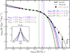 |
Fig. 8. Variation in the best-fit double Schechter function resulting from three different parameterisations of the uncertainty in ℳ used for the Eddington bias kernel (Eq. (11)) at 1.1 < z ≤ 1.5. The shape of the kernel according to each parameterisation is shown in the inset plot, with the corresponding parameter values annotated above in matching colours. The resulting intrinsic (solid) and observed (dotted) galaxy SMF is shown for each case, with the value of the best-fit characteristic mass (ℳ★) annotated and given by the vertical dashed lines. The treatment of the Eddington bias significantly affects the inferred intrinsic galaxy SMF. |
Figure 8 also demonstrates that the treatment of the Eddington bias used herein is sufficient to characterise the observed excess of massive galaxies at 1.1 < z ≤ 1.5 (similar behaviour is seen in the next two redshift bins as well). Although the values of the Eddington bias parameters (σEdd, τEdd) were not selected by visual comparison, Fig. 8 nonetheless shows a very good agreement between the observed data and the intrinsic SMF that results from the fit that uses σEdd = 0.6 and τEdd = 0.05(1 + z). By contrast, larger values over-predict the number density of observed massive galaxies, while smaller values under-predict. Indeed, comparing the χ2 of each fit, the smallest values achieve the worst reduced-χ2 value at 4.23. The other two achieve similar χ2 values at 1.72 for the values used herein and 1.68 for the largest kernel assumed. Despite the marginal improvement in the χ2, there appears to be no reason to prefer the larger kernel, as it is not supported by the measured posterior distributions of ℳ and it appears to over-predict the abundance of observed massive galaxies.
5.4.2. Degeneracy of model parameters
Independent of the Eddington bias, it is well known that there exists a degeneracy between the low-mass slope α, the turnover mass or knee, ℳ★, and the normalisation Φ* (see, for example, Fig. 8 of Stefanon et al. 2021 or Fig. 7 of W24). The DAWN PL mass completeness limit is already nearly ℳ ∼ 1010 M⊙ by z ∼ 2, and therefore DAWN PL cannot constrain the galaxy SMF at low masses. Nonetheless, it should still be possible to constrain the knee or characteristic mass, ℳ★, as well as the overall normalisation, Φ*. Consequently, the low-mass slope is handled differently than the other Schechter parameters during the modelling step.
It is emphasised that there is no solution that is completely free of assumption for modelling a parameter that is not well constrained by the data. One option is to freeze the low-mass slope throughout the modelling step and only fit for the characteristic mass and the normalisation, an option typically used in modelling the highest redshifts included by the given selection function (Davidzon et al. 2017; Weaver et al. 2023a; Weibel et al. 2024). Alternatively, a prior may be used to restrict the allowable values of the low-mass slope while still accounting for some of the covariance between the Schechter parameters and the resulting uncertainty of their inferred values. The latter approach is used herein. In each redshift bin, a flat prior motivated by results from the literature is used, and the range of allowed values evolves with redshift.
Table 2 lists the ranges of low-mass slopes allowed in fitting. At z ≤ 2.5, the low-mass slope α lies within the range −1.55 < α < −1.3, consistent with both D17 and W23. At higher redshifts (z > 2.5), W23 held α fixed to the value determined in the 2.0 < z ≤ 2.5 interval, while D17 allowed it to vary freely, finding steeper values at z > 2.5. In this work, we allowed α to vary at high redshifts and find that it steepens accordingly. At 2.5 ≤ z < 3.5, the permitted range is −1.7 < α < −1.45, consistent with both prior studies. For 3.5 ≤ z < 4.5, we find a range of −1.85 < α < −1.65, diverging from W23 but remaining in agreement with D17, as well as the high-redshift constraints from G15 and W24. At the highest redshifts (z ≥ 4.5), the allowed interval broadens to −2.2 < α < −1.65, accommodating the steeper slopes reported by G15, D17, and W24.
Allowed ranges for the faint-end slope (α) in different redshift bins.
For double-Schechter models, the above prior is only imposed on the low-mass slope α1, while the slope of the second Schechter component, α2, is free to vary. As the low-mass end of the galaxy SMF is dominated by star-forming galaxies, the star-forming and total galaxy SMFs are modelled using the same priors on the low-mass slope, keeping in mind that the star-forming galaxy SMF is considered separately only below z = 3. For the same reason, the low-mass slope of the quiescent SMF is handled differently, using different ranges of allowable values for α. At z < 1.1, the range of allowed values is −2.5 < α < 0, while at z ≥ 1.1, the range of allowed values is 0 < α < 2.5. In both cases, the range of allowed values is quite broad but nonetheless provides useful boundaries that are consistent with both D17 and W23. Effectively, the prior requires that the slope is negative at z < 1.1 and positive at z > 1.15.
The above handling of α encourages a physically plausible evolution of the galaxy SMF to result from the fitting procedure. An additional requirement is imposed following W23, in which an upper limit is placed on the normalisation Φ* of the galaxy SMF. For every bin above the first redshift bin (0.2 < z ≤ 0.5), the normalisation of the galaxy SMF is required to be less than or equal to the 84% percentile (corresponding to +1σ for a Gaussian distribution) of the posterior distribution of Φ* from the previous redshift bin, Φ84*. For double-Schechter models, both Φ1* and Φ2* are required to be less than max(Φ1, 84*,Φ2, 84*). This additional prior, like the prior on α, is physically motivated and also discourages an evolution of the intrinsic galaxy SMF in which the total SMD (Sect. 6.1) decreases as the amount of time since the Big Bang grows. In all cases, Φ* is found to decrease with redshift as expected.
5.5. Markov chain Monte Carlo analysis
In order to consider a range of possible values for the Schechter parameters and determine useful uncertainties on the representative values, the observed galaxy SMF is fitted in a MCMC approach based upon emcee (Foreman-Mackey et al. 2013) following the process outlined in W23. Initial values are determined by first fitting each of the total, star-forming, and quiescent galaxy SMFs via a χ2 minimisation with the same priors discussed above. As emcee enables ensemble sampling, a collection of 500 MCMC ‘walkers’ are initialised based on the best-fitting values from the χ2 minimisation but scattered within 2%. The walkers explore the parameter space simultaneously via multi-processing and for as many steps as required to each beyond 10× their autocorrelation length. An additional requirement is that the estimated autocorrelation length is not changing more than 1%. These criteria measure ensures that each Markov chain has satisfactorily converged and that the total area explored is not dictated by the initial conditions.
Two sets of Schechter parameters are obtained from the MCMC analysis. The first correspond to the median of the marginalised posterior distributions of each parameter. The second corresponds to the maximum a posteriori parameters. As described by W23, these two sets of parameters provide different descriptions of the intrinsic galaxy SMF. The former is often used in the literature and describes parameter values that are frequently encountered during the sampling, implying that they may be representative due to their prevalence. However, the set of parameters defined by the median of each marginalised posterior distribution does not necessarily correspond to parameter values that are encountered simultaneously with each other, and therefore they are not guaranteed to provide a good fit (high likelihood) to the data. One of the appeals of using the median of the marginalised posterior distributions is that the uncertainty on a given parameter may be meaningfully determined from the percentiles of the posterior distribution. By contrast, the maximum a posteriori parameters provide a model that most closely resembles the data given the likelihood function and any assumed priors. The downside is that there is no single method for obtaining uncertainties on their values. Accordingly, caution is advised when considering either set of Schechter parameters. Each set of parameters is presented in Table A.1 for the total SMF, Table A.2 for the star-forming SMF, and Table A.3 for the quiescent SMF.
The intrinsic total galaxy SMF for all redshift bins is shown in Fig. 9 according to the maximum a posteriori parameter values, while Fig. 10 shows the same for the intrinsic star-forming and quiescent SMF but restricted to z ≤ 3. As should be expected, the variation is greatest at z > 4.5 where the total uncertainties (σtot) are weakest and the mass completeness limit is highest (ℳ > 1010 M⊙). In comparison to the observed SMF, the intrinsic SMF differs most strongly on the massive end. This is due to the effect of the Eddington bias kernel, which results in an intrinsic SMF that does not necessarily trace the most massive bins, as demonstrated by Fig. 8. Whether the abundance of such massive galaxies is driven by the uncertainty in ℳ, as assumed by the Eddington bias kernel, or the abundance of the most massive systems is accurate, is further discussed in Sect. 6.4.
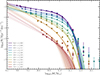 |
Fig. 9. Evolution of the intrinsic galaxy SMF of the total sample, shown as solid lines, across 0.2 < z ≤ 6.5. Maximum a posteriori values are assumed, as listed in Table A.1. The 1σ (2σ) uncertainty according to the variation in the MCMC chains is shown by the dark (light) shaded regions. Extrapolations below the stellar mass limit (Eq. (3)) are shown by the dashed lines, and the uncertainties are indicated by the hatched regions. Observed values for corresponding redshift bins are shown in the matching colour as data points with error bars. |
The goal of this work is not to investigate a possible evolutionary trend in the Schechter parameters that describe the intrinsic SMF. Instead, the Schechter function formalism is primarily useful for empirically describing the shape of the intrinsic SMF by enabling a straightforward accounting of the Eddington bias through forward modelling. Nonetheless, a brief comparison to the literature of the representative values found at each redshift is warranted because it may validate the modelling procedure and the decisions regarding the treatment of the Eddington bias. This comparison is provided in Appendix A. Overall, the comparison shows broad agreement with the literature, with disagreement mostly explained by the covariance of the Schechter parameters and stellar mass ranges explored by each dataset. Future works that seek to investigate an evolution in the Schechter parameters or perform detailed comparisons with the literature should take effort to account for both the differences in assumptions of the Eddington bias and for the covariance between the Schechter parameters.
The star-forming component of the intrinsic SMF is depicted in the left panel of Fig. 10, while the quiescent component is shown in the right panel. Both the star-forming and quiescent components are shown at z ≤ 3, keeping with the separation defined in Sect. 3.2. Generally, the star-forming component resembles the total SMF. The quiescent SMF, on the other hand, is quite different, perhaps most uniquely characterised by a low-mass slope that increases with redshift. In contrast to the star-forming and total SMF, the intrinsic quiescent SMF suggests that the quiescent galaxies below the characteristic mass are rare in the early Universe, but become increasingly more common at late times. Despite the lack of constraints on the low-mass end of the quiescent SMF, the inferred Schechter parameters are mostly supported by D17 and W23. The primary difference is in the normalisation, where a smaller value is typically found in DAWN PL in accordance with the differences in completeness discussed in Sect. 3.2. In addition, the value of ℳ★ is higher in DAWN PL at z > 1.5. This is driven by both the stellar mass limit, which is log10(ℳ/M⊙) > 10.5 at z > 1.5, and the abundance of massive quiescent galaxies that exceeds both D17 and W23 at these redshifts. As discussed in Sect. 3.2, the intrinsic quiescent SMF also suggests that a significant fraction of the most massive quiescent galaxies, for example log10(ℳ/M⊙) > 11.5, had already formed by z∼ 2–3, just 2–3 Gyr after the Big Bang. Massive quiescent galaxies at z > 2 are discussed in greater detail in Sect. 6.4.
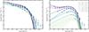 |
Fig. 10. Same as Fig. 9 but separated into star-forming (left) and quiescent galaxies (right) at z ≤ 3. |
6. Discussion
The galaxy SMF is commonly used as a tool to constrain the cosmic SMD. This section includes a validation of the evolution of the galaxy SMF measured and implied cosmic SMD through a comparison with similar efforts in the literature. However, perhaps the greatest difference between DAWN PL and previous works is the volume explored to high redshifts. As seen in Sect. 5, the increased volume leads to smaller uncertainties regarding the abundance of the most massive galaxies, especially at z > 3.5. The implications of these galaxies and the connection to their host dark matter halos and their environments is explored in this section. Additional systematics and interloper populations are further discussed, along with a presentation of a few select massive galaxies.
6.1. Cosmic stellar mass density
The cosmic SMD (ρ★) describes the total stellar mass, provided by all galaxies, per unit volume. A determination of the implied value of ρ★ at each redshift can be obtained by integrating the intrinsic SMF at that redshift, multiplied by ℳ, over an appropriate range of stellar mass. A related quantity is the cosmic star formation rate density (SFRD), which describes the star-formation rate over all galaxies per unit volume. The SFRD can be determined by multiple independent methods. For example, the SFRD may be measured from UV measurements (Cucciati et al. 2012), far-infrared (FIR) measurements (Gruppioni et al. 2013), millimetre and radio measurements (Le Borgne et al. 2009; Dunne et al. 2009), and even gamma ray bursts (Kistler et al. 2013). The SFRD can be converted to the corresponding SMD by assuming a particular IMF for star formation and by characterising the fraction of stellar mass that is lost due to stellar evolutionary processes. A notable example of this procedure is demonstrated by Madau & Dickinson (2014). Consequently, measuring the SMD provides an opportunity to compare the various methods for measuring stellar mass growth in galaxies across cosmic time.
As described above, a measurement of ρ★ can be obtained directly from the inferred intrinsic SMF obtained in Sect. 5.4. In the literature, the most commonly used range of integration is 108 < ℳ/M⊙ < 1013. Therefore, the same interval is considered in this work to provide an estimate of the implied evolution of ρ★. A comparison with values from the literature is provided in Fig. 11. All reported values from the literature have been converted to a Chabrier IMF and integrated across 108 < ℳ/M⊙ < 1013.
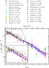 |
Fig. 11. SMD, ρ★, obtained from integrating the intrinsic galaxy SMF (from ℳ = 108 M⊙ to ℳ = 1013 M⊙), shown for both the median posterior values (circle symbols and solid line) and the maximum a posteriori values (square symbols). Values are compared with measurements from the literature also derived from galaxy SMFs (Caputi et al. 2011; González et al. 2011; Santini et al. 2012; Ilbert et al. 2013; Muzzin et al. 2013; Tomczak et al. 2014; Grazian et al. 2015; Caputi et al. 2015; Wright et al. 2018; Bhatawdekar et al. 2019; Adams et al. 2021; McLeod et al. 2021; Thorne et al. 2021; Stefanon et al. 2021; Weaver et al. 2023a; Weibel et al. 2024; Shuntov et al. 2025) as well as integrations of the cosmic SFRD functions (Madau & Dickinson 2014; Behroozi et al. 2019). For the latter, a return fraction of 41% (based on the Chabrier 2003 IMF; see Sect. 6.1 of Ilbert et al. 2013) is assumed. For Madau & Dickinson (2014), a shaded area is shown corresponding to return fractions between 25–30% (where the latter value is similar to the Salpeter 1955 IMF). |
From 0.2 < z ≲ 6, the evolution of ρ★ agrees well with the literature (G15, D17, W23, W24). At z ∼ 4, the same is true, although W23 measures a slightly lower value, likely caused by their lower value of the low-mass slope, α. Given the power-law shape of the low-mass end of the SMF and the exponential decline at high masses, ρ★ is significantly more sensitive to the characterisation of low-mass galaxies compared to massive galaxies. Thus, despite the abundance of massive galaxies that require extreme star-formation efficiencies at z > 3.5, their contribution to the SMD is dwarfed by galaxies with lower stellar masses. At z ≲ 4, DAWN PL remains consistent with both D17 and W23, except at the redshift bin corresponding to z ≤ 1.5. At these lower redshifts, the difference in the selection of quiescent galaxies like causes a small discrepancy of less than a factor of 2. Note that at z ≤ 0.8, DAWN PL finds a slightly greater value of ρ★, which may be due to the larger volume of DAWN PL that includes a great sampling of large-scale structure compared to COSMOS.
The broad agreement between the values of ρ★ measured from DAWN PL and the literature at-large validates the modelling procedure of Sect. 5.4, and in particular, the treatment of the low-mass slope α. Interestingly, at z > 2.5, comparison across the different works appears to show an agreement in the value of ρ★ that increases with publication date. In other words, the measurements that demonstrate the greatest deviations at z > 2.5 are also some of the earliest (e.g. before 2014). This likely reflects the improvement in data quality and may also suggest that observational methods for selecting and characterising galaxies at high redshifts since improved or at least have become more uniform. At z ≤ 2.5 a substantial fraction of the datasets, including this work, provide estimates of ρ★ that are lower than the values reported by Madau & Dickinson (2014) and Behroozi et al. (2019), at least until z ∼ 0.5. Both Madau & Dickinson (2014) and Behroozi et al. (2019) measure the SMD by converting measurements of the SFRD across redshifts using an assumed return fraction. Consequently, the origin of this discrepancy is not obvious, although there are many possible explanations explored by Madau & Dickinson (2014).
6.2. Galaxy-dark matter connection
A pillar of modern studies of galaxy evolution holds that galaxies form and evolve within dark matter halos. Consequently, the evolution of galaxies is directly linked to the evolution of their host dark matter halos (Wechsler & Tinker 2018). This relationship is generally referred to as the galaxy-halo connection. Numerous techniques are used in the literature to connect galaxies to dark matter halos, for example, hydrodynamical simulations (Vogelsberger et al. 2014; Schaye et al. 2015, 2023), semi-analytic models (Guo et al. 2011; Henriques et al. 2015), empirical forward modelling (Behroozi et al. 2013, 2019), abundance matching (Marinoni & Hudson 2002; Stefanon et al. 2021), and halo occupation distribution modelling (Harikane et al. 2018; Shuntov et al. 2022). The mass of the host dark matter halo appears to be the dominant intrinsic property with which many aspects of evolution are correlated (e.g. Contreras et al. 2015; Man et al. 2019). Consequently, it is often a goal to measure the stellar-to-halo mass relation (SHMR), which describes the stellar mass of galaxies as a function of the dark matter halo mass. While a detailed analysis involving the methods described above is beyond the scope of the present work, a qualitative comparison can easily be made by comparing the intrinsic SMF with the dark matter HMF.
Like the galaxy SMF, the dark matter HMF describes the co-moving number density of dark matter halos as a function of dark matter halo mass. The HMF can be roughly translated into a predicted SMF by assuming a baryon fraction and an integrated star-formation efficiency, ϵ. In SHMR studies, the value of a galaxy’s ratio of stellar mass to dark matter halo mass defines the integrated star-formation efficiency, i.e. ℳ/(ℳhfb)≡ϵ, where fb ≡ Ωb/Ωm = 0.166 is the fraction of baryonic matter in the Universe. Consequently, the integrated star-formation efficiency should be thought of as the time-averaged efficiency by which baryons have been converted into stars over the lifetime of the host halo, in contrast to an instantaneous star-formation efficiency (SFR/ ) or a gas-depletion efficiency (SFR/ℳgas).
Figure 12 shows the intrinsic SMF and observations at 0.2 < z ≤ 3.5 compared to the HMF of Tinker et al. (2008). In each panel, the coloured solid curve represents the maximum a posteriori SMF, while the coloured dotted curve represents the equivalent for the observed SMF, i.e. the Schechter function (or double-Schechter function) convolved with the Eddington bias kernel of Eq. (11). The HMF is scaled assuming a constant baryon fraction and three different values of ϵ: ϵ = 0.10, ϵ = 0.25, and ϵ > 1. The parameter space spanned by ϵ > 1 indicates the stellar mass of galaxies that are disallowed by the assumptions of the HMF and a universal value of fb, as the formation of any galaxy with such a stellar mass would have required more baryonic matter than is available. The comparison with the scaled HMF at z ≤ 3, shown in Fig. 12, suggests that galaxies at low-stellar masses and very high-stellar masses both suffer very low integrated star-formation efficiencies, as has been found in virtually all recent characterisations of the SHMR (Wechsler & Tinker 2018 and citations therein). At low stellar masses, star formation can be suppressed by internal processes regulated by stellar feedback including photoionisation, supernovae, and stellar winds (e.g. Hopkins et al. 2012). At high stellar masses, feedback mechanisms driven by AGN and virial shock heating can suppress star formation (e.g. Vogelsberger et al. 2013). Galaxies near the characteristic ℳ★ of the Schechter function achieve the maximum ϵ between 10% and 25%. In SHMR analyses, the ℳ at which galaxies achieve the maximum ϵ is referred to as the ‘pivot-mass’. Galaxies at the pivot-mass are those that have been the most efficient at converting baryons into stars over the lifetime of the halo. Their host dark matter halos were massive enough to withstand stellar feedback but not yet massive enough to have developed dominant AGN components or to shock-heat in-falling gas.
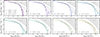 |
Fig. 12. Intrinsic galaxy SMF of the total sample through to 3.0 < z ≤ 3.5 (solid lines) and observed values (data points) with error bars (in matching colours) compared to the Tinker et al. (2008) dark matter HMF assuming a universal baryon fraction and various integrated star-formation (baryon-to-star conversion) efficiencies, ϵ. ℳ bins below the stellar mass limit are not shown. Maximum a posteriori values for the intrinsic galaxy SMFs are assumed. The uncertainty (1σ dark, 2σ light) according to the variation in the MCMC chains is shown by the shaded regions. The dotted coloured line represents the ‘observed’ model of the galaxy SMF, i.e. including the Eddington bias (Sect. 4.3). The shaded grey region corresponds to the number density of galaxies that would require 100% conversion (or greater) of baryons into star. |
At z ≤ 3, massive galaxies with ℳ > ℳ★ are characterised by lower values of ϵ than those with ℳ ∼ ℳ★. However, at 3 < z ≤ 3.5, the intrinsic SMF suggests a change in the SHMR compared to low redshifts. At 3 < z ≤ 3.5, essentially all galaxies observed above ℳ★ exhibit integrated star-formation efficiencies greater than or equal to 25%. The maximum a posteriori model of the observed SMF, shown by the coloured dotted line, suggests that the abundance of the most massive systems is over-estimated due to uncertainties in their stellar masses. Even so, the area enclosed at ϵ > 0.10 by the intrinsic SMF (in which the Eddington bias has been removed) is significantly greater than at lower redshifts and includes galaxies of greater stellar mass. The increased average ϵ achieved by massive galaxies would therefore manifest in a broader peak in the SHMR, where a range of galaxy stellar masses are characterised by the maximum integrated star-formation efficiency. The work best-suited to validate this suggestion is Shuntov et al. (2022), wherein the authors performed a detailed halo-occupation distribution modelling of galaxies selected from the COSMOS2020 catalogue. In this way, it is naturally complimentary to W23, which agrees very well with the observations from DAWN PL at 3 < z ≤ 3.5 (Fig. 5). Notably, Shuntov et al. (2022) is the only work to have measured the SHMR to high z (z ≤ 5.5) using a large survey area (> 1 deg2), reliable photo-zs, and galaxy stellar masses constrained by IR observations. Indeed, the authors find that the peak of the SHMR becomes substantially broader at z > 2.5, albeit with non-negligible uncertainty. A similar result was obtained by Harikane et al. (2018) from an even larger area (∼100 deg2), although the redshifts and stellar masses of the galaxies are significantly more uncertain due to a lack of rest-frame optical constraint from IR data.
Another result of Shuntov et al. (2022) suggests that at z > 3, the most massive galaxies have larger ratios of stellar-to-dark matter halo mass compared to those at lower redshifts (i.e. they achieve greater overall integrated star-formation efficiencies). Although a careful determination of the host dark matter halos is required to say conclusively, this scenario is consistent in principle with the comparison of the SMF from DAWN PL at 3 < z ≤ 3.5 and the HMF. However, Shuntov et al. (2022) further suggests that both effects, an increased fraction of stellar mass compared to dark matter halo mass, and a broader range of stellar masses achieving high integrated star-formation efficiencies, become stronger with increasing redshift. Figure 13 compares the intrinsic SMF and observations at 3.5 < z ≤ 6.5 compared to the Tinker et al. (2008) HMF. In Fig. 13, two additional scalings of the HMF are shown, ϵ = 0.50 and ϵ = 0.75. The comparison of the intrinsic SMF and the scaled HMF at 3.5 < z ≤ 4.5 is mostly similar to 3.0 < z ≤ 3.5 but now includes galaxies that achieve an even greater integrated star-formation efficiency, in excess of ϵ = 0.25 and approaching ϵ = 0.50. As demonstrated by the agreement between the present observations and both G15 and D17 in Fig. 6, such galaxies have been observed before. Indeed, although their abundance may seem excessive, it is emphasised that W23 found an even greater abundance of galaxies requiring large integrated star-formation efficiencies (see W23, Fig. 17). The difference between the present work and these references is the greater statistical significance of their abundance, which is discussed further below. For comparison, Shuntov et al. (2022) suggests that massive galaxies at 3.5 < z ≤ 4.5 may achieve integrated star-formation efficiencies that are a factor of ∼2 greater than those at z ≤ 3, which is consistent with the ϵ required by the most massive galaxies observed in DAWN PL.
The comparison between the intrinsic SMF and the HMF becomes more difficult at z > 4.5, where the inability to detect galaxies with low stellar mass weakens the constraints of the Schechter parameters. Consequently, there is some uncertainty in the shape of intrinsic galaxy SMF above log10(ℳ)/M⊙) > 11. In any case, at 4.5 < z ≤ 5.5, there are galaxies observed that require ϵ > 0.50, and even ϵ ≥ 0.75. This remains consistent within the 1σ upper bound of the SHMR of Shuntov et al. (2022), where the authors found that the SHMR does not change significantly between z ∼ 4 and z ∼ 5. Galaxies of approximately log10(ℳ/M⊙)∼11.5 require ϵ ∼ 0.50, according to the observations shown in Fig. 13. The abundance of galaxies around this stellar mass is supported by W23 and W24, and W23 actually suggests an even greater abundance of these galaxies (see again, Fig. 17 of W23 and their Sect. 6.3, and also W24, Fig. 11) therefore requiring an even greater integrated star-formation efficiency. However, these works do not find galaxies of greater stellar mass. One galaxy, with a statistical significance that does not exceed the 1σ upper bound for N = 0 detections, is found with ϵ > 1. This galaxy is discussed Sect. 6.4. The trend continues 5.5 < z ≤ 6.5 where again there are galaxies that require ϵ ≥ 0.75. Generally, the abundance of such galaxies is consistent with both W23 and W24, though it is noted that this comparison is highly uncertain, as neither of these two works can do more than provide upper limits on the abundance of galaxies with these stellar masses log10(ℳ/M⊙) > 10.75 (see Fig. 6).
The existence of a substantial population of galaxies at z ∼ 5–6 with integrated star-formation efficiencies of ϵ ≫ 0.25 implies that the feedback mechanisms that inhibit star formation in massive galaxies at lower redshifts are not as effective in the early Universe. To start, it is expected that these massive systems reside in dark matter halos in which feedback from stellar evolution (e.g. supernovae) is not efficient. From a theoretical perspective, Bassini et al. (2023) developed simulations in the Feedback In Realistic Environments (FIRE) project (Hopkins et al. 2014, 2018) to assess the possible impact of stellar feedback on star formation in massive galaxies ( ) at z ≥ 5.5. Indeed, the authors found that stellar feedback is extremely inefficient for regulating star formation due to the significant gas surface densities common at these redshifts (102–103 M⊙ pc−2), and that gas is consumed by star formation on shorter timescales (gas depletion time ∼20 Myr) than it can be expelled. However, in less massive galaxies (ℳ < 1010 M⊙), stellar feedback regulates star formation. Although perhaps coincidental, this is very nearly the value at which the intrinsic and observed SMF goes below ϵ = 0.10 in Fig. 13.
As discussed above, AGN activity is commonly cited as the primary factor inhibiting star formation in massive galaxies (Wechsler & Tinker 2018 and references therein). However, a quantitative and detailed understanding of AGN feedback at high redshifts that is empirically confirmed is not yet developed. To measure the impact of AGN feedback at lower redshifts (z ≤ 2.5), Fiore et al. (2017) used a combination of measurements from molecular, ionised, broad absorption line, and X-ray winds and found that only galaxies with ℳ ≥ 1011 M⊙ at z ≤ 2 are capable of driving mass outflows rates that exceed the star-formation rate with a trend that decreases with increasing redshift. Through observation, it is difficult to fully assess the effects of outflows in galaxies at z ∼ 5–6. At z ≥ 5 FIR observations with high-resolution and depth are necessary to detect outflows and measure their spatial distributions (Fujimoto et al. 2019), making statistical arguments difficult due to small sample sizes. Valentini et al. (2021) produced simulations of massive galaxies (ℳh = 1012 M⊙) at z = 6 using GADGET3, a private successor to GADGET2 (Springel et al. 2005), with detailed characterisation of AGN activity. Ultimately, the authors found that AGN feedback could not significantly halt the inflow of cold gas or influence the star-formation history of the galaxy, even when manually increasing the efficiency of AGN feedback by a factor of 10.
Observations at lower redshifts have historically implied a period of enhanced star-formation efficiency for the most massive galaxies in the early Universe (Cowie et al. 1996). For example, should massive galaxies at z > 3.5 undergo a period of enhanced star-formation efficiency, then it should be expected that a substantial abundance of massive quiescent galaxies is observed some time thereafter. Indeed, the evolution of both the observed quiescent SMF (Fig. 7) and the intrinsic quiescent SMF (Fig. 10) suggest that a significant fraction of the most massive quiescent galaxies are already in place by z ∼ 2.5, just 2.57 Gyr after the Big Bang. Quiescent galaxies at this mass do not appear to substantially grow in abundance from then onwards, nor does it appear that more massive quiescent systems arise later. Accordingly, the effects of AGN feedback, which were not yet strong enough to inhibit star formation at high z, may be delayed (e.g. D17,Valentini et al. 2021). By z ∼ 2 at least, these systems are more massive than the minimum stellar mass found by Fiore et al. (2017) that is needed for AGN feedback to completely ‘clean’ galaxies of their molecular gas. Assuming feedback is strong and gas supplies are absent, the only evolutionary pathway for such systems to grow in abundance is through merging events. Mundy et al. (2017) showed that on average, galaxies with ℳ > 1011 M⊙ undergo approximately 0.5 major mergers across 0 < z ≤ 3.5, a process that typically adds 1–4 ×10¹⁰ M⊙. Minor mergers should also be considered and are important at low z (Jespersen et al. 2022; Chuang et al. 2024), but it is difficult to measure their impact at high z (Lotz et al. 2010). Conselice et al. (2022) found a slightly greater major merger rate at ∼0.84 than Mundy et al. (2017) and also found that the growth in stellar mass for the same galaxies is approximately a factor of 2 (0.3 dex). The evolution in the shape of the observed quiescent SMF (Fig. 7) and total SMF with respect to the scaled HMF is consistent with this picture of little to no growth in the abundance of the most massive galaxies. This was found by Kawinwanichakij et al. (2020) this results extends the finding to z ∼ 2.5 and tentatively higher, considering the total sample.
Recent observations of exceptionally massive galaxies from JWST at z > 8 and above (Harikane et al. 2023; Casey et al. 2024; Weibel et al. 2024) imply the existence of similarly massive galaxies at later times. For example, W24 finds several galaxy candidates at z ∼ 8–9 that would require equal or greater integrated star-formation efficiencies to those found in DAWN PL. In addition, Casey et al. (2024) reports the discovery of three candidate galaxies at z ∼ 12 with ℳ ∼ 4–10 × 109 M⊙. These systems require extreme evolutionary histories acting on short timescales. Several possible theories have been put forth to explain them, including ‘feedback-free’ bursts of star formation (Dekel et al. 2023; Li et al. 2024) and positive feedback from AGNs (Silk et al. 2024). Without a measure of current star-formation activity in the massive galaxies found in DAWN PL, there is a degeneracy among evolutionary histories that would yield similar values of ϵ required for them to form, given that ϵ is a quantity that is integrated over the entire evolutionary timescale of the host halo. Spectroscopic confirmation, and a spectro-photometric analysis, is ultimately required to understand the nature of these massive galaxies in detail.
6.3. Galaxy environment
The results discussed in Sect. 6.2 motivate investigation of a possible correlation between galaxy stellar mass and the local density field, or environment. The SHMR (Wechsler & Tinker 2018; Behroozi et al. 2019; Shuntov et al. 2022) and other observations, for example galaxy bias (Beck et al. 2020), show that the galaxies with the greatest stellar mass must also reside in the most massive dark matter halos. In the early Universe, the most massive dark matter halos are also the sites of large-scale structure formation (Springel et al. 2006; Porqueres et al. 2019). Consequently, there is reason to suspect a relationship between stellar mass and environment, even at high z.
Determining the role of the environment in affecting galaxy evolution has been a topic of study for decades (e.g. Oemler 1974; see also Conselice 2014 and citations therein). Although environments may be characterised in different ways, it is common to describe environment in relation to the local density by measuring the relative ‘overdensity’, which is the difference in the local density compared to the average density; this is the definition used herein. Advancements in galaxy surveys across the past two decades have enabled studies seeking to link the role of environment in galaxy evolution, specifically through its impact on the galaxy SMF (Bundy et al. 2006; Bolzonella et al. 2010; Peng et al. 2010). These early works showed a greater abundance of massive galaxies in high-density environments. Peng et al. (2010), in particular, introduced the concepts of ‘environmental quenching’ and ‘mass quenching’ which are now commonly used to describe two different ways galaxies are thought to transition from star-forming to quiescent. This has also been investigated in low-z simulations, where Wu & Kragh Jespersen (2023), Wu et al. (2024) find strong environmental dependencies in galaxy properties.
At redshifts z > 1 it has generally been a challenge to measure the galaxy SMF as a function of environment because the high-redshift surveys were either too small in area to sample cosmologically distinct environments or did not have the necessary IR wavelength coverage (e.g. from Spitzer/IRAC) to reliably measure stellar masses at high z. Nonetheless, efforts to measure the impact of environment on the resulting galaxy SMF at higher redshifts are continually improving. As a few examples, Bolzonella et al. (2010) used some ten thousand galaxies from zCOSMOS (Lilly et al. 2007) sampling a 1 deg2 area to z ∼ 1; Etherington et al. (2016) used several million galaxies across a few hundred deg2 of the Dark Energy Survey (DES; Dark Energy Survey Collaboration 2016) to z ∼ 1; Davidzon et al. (2016) used 50 000 galaxies from the VIMOS Public Extragalactic Redshift Survey (VIPERS; Guzzo et al. 2014) spanning 0.5 < z < 1; Tomczak et al. (2017) analysed galaxies selected from 8 individual fields, each spanning between ∼150–450 arcmin2, of the Observations of Redshift Evolution in Large-Scale Environments survey (ORELSE; Lubin et al. 2009) at 0.6 < z < 1.3; Kawinwanichakij et al. (2017) used galaxies selected from the ∼300 arcmin2 FourStar galaxy evolution survey (ZFOURGE; Straatman et al. 2016) out to z ∼ 2; Papovich et al. (2018) used the same galaxies at Kawinwanichakij et al. (2017) as well as an additional sample selected from the Newfirm Medium Band Survey (NMBS; Whitaker et al. 2011) spanning ∼1500 arcmin2 again to z ∼ 2; Forrest et al. (2024b) considered two individual protoclusters at z ∼ 2 and at z ∼ 3 selected from COSMOS2020 (Weaver et al. 2022); and Edward et al. (2024) studied the queiscent galaxy SMF in protoclusters at z ∼ 2 − 2.5.
Future investigations will undoubtedly make use of DAWN PL’s significant volume, the imminent grism spectroscopy from Euclid (Euclid Collaboration: Scaramella et al. 2022), and reliable stellar masses provided by the deep Spitzer/IRAC data to explore many facets of galaxy evolution in relation to the environment. Although such detailed analyses are currently beyond the scope of this work, enough physical parameters have already been measured and formalisms defined to obtain a simple estimate of the abundance of galaxies as a function of their stellar mass and environment. It should be noted that despite the uniquely large area and rest-optical coverage at these redshifts, the limiting factor in this preliminary investigation is the photometric redshift precision, relative to similar, spectroscopically based studies in the literature.
The local density of every galaxy is estimated using a simplified implementation of the procedure described by Kovač et al. (2010) for measuring the density field of the zCOSMOS spectroscopic sample (Lilly et al. 2007) over a 1 deg2 area. The same measurements were used by Peng et al. (2010). Following Kovač et al. (2010), the local density around each galaxy is estimated using an aperture of variable size. The radius of the aperture is determined by the distance to the Nth nearest neighbour, where N = 5 (Kovač et al. 2010; Peng et al. 2010; Davidzon et al. 2016). The local density measurement is thus  , where d5 is the projected distance to the 5th nearest neighbour. Galaxies are each given equal weight such that the resulting density measurement simply describes the counts of objects within the aperture to avoid biasing the overdensity measurement around central objects of significant stellar mass (Kovač et al. 2010). For the tracer sample, all galaxies above the stellar mass limit (Sect. 3.3) are used for simplicity and consistency with the above selections (Sect. 3.1) of galaxies used to construct the SMFs. Galaxies are also binned according to the redshift binning used throughout (i.e. Table 1). Note that this redshift spacing is approximately similar to the spacing used by Papovich et al. (2018). Each galaxy is assigned an overdensity value, δ, which is the difference between the density measured at the position of the galaxy and the average density considering all galaxies and their respective density values, divided by the average density. Finally, galaxies are grouped into quartiles of overdensity based on the distribution of log10(1+δ).
The galaxy SMF is measured across each redshift bin and for each density quartile. Uncertainties σΦ in each ℳ bin are computed as described in Sect. 3.4, and volumes treated as described in Sect. 4. As is commonly done in the literature, the change in the shape of the galaxy SMF is measured by comparing the resulting SMFs from the most dense quartile, D4, to the least dense quartile, D1. Similar to Tomczak et al. (2017), the ratio of each SMF is measured here for each redshift bin considered. The result is summarised in Fig. 14. The y-axis is given by
 (12)
(12)
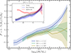 |
Fig. 14. Fraction of all galaxies in each ℳ bin in the most dense environments, D4, compared to the least dense environments, D1, relative to unity, ℱ = 1 − N(D1)/N(D4). See the main text for a description of the density estimates. For ℱ < 0, more galaxies are contributed by the least-dense environments; ℱ = 0 implies the two quartiles contribute equally; and ℱ > 0 indicates that more galaxies are contributed by the most dense environments. The solid coloured lines indicates the ratio of the counts in each quartile (subtracted from 1), and the shaded regions correspond to the 1σ uncertainties propagated from σΦ (Sect. 3.4). At low masses (ℳ < 1010 M⊙), more galaxies are found in low-density environments, while galaxies above are preferentially located in high-density environments. The inset plot shows the same relationship for 0.8 < z ≤ 1 separated into star-forming and quiescent galaxies. The over-abundance of low-mass quiescent galaxies in high-density environments is indicative of ‘environment quenching’ (Peng et al. 2010, 2012). |
where ℱ is the fraction of galaxies contributed to each ℳ bin by the most dense quartile relative to unity. For example, at ℱ < 0, more galaxies are contributed by the least-dense environments; ℱ = 0 implies the two quartiles contribute equally; and ℱ > 0 indicates that more galaxies are contributed by the most dense environments. The solid coloured lines represent the ratio of the counts in each quartile (subtracted from 1), and the shaded regions correspond to the 1σ uncertainties propagated from σΦ (Sect. 3.4). The two lowest-redshift bins 0.2 < z ≤ 0.5 and 0.5 < z ≤ 0.8 are not shown as they show no considerable change compared to 0.8 < z ≤ 1.1. However, the increased abundance of massive galaxies in dense environments is obvious at these low redshifts and is generally reminiscent of Peng et al. (2010) and the other low-redshift works. Thus, Fig. 14 begins with 0.8 < z ≤ 1.1 to provide a point of comparison with recent works (Etherington et al. 2016; Tomczak et al. 2017; Papovich et al. 2018) reaching to higher redshifts. In the primary area of the figure, the value of ℱ is given for the total SMF for each of the redshift interval shown.
Figure 14 shows that the abundance of galaxies as a function of stellar mass depends on the local environment, at least from 0.8 < z ≤ 1.1 out to 3.0 < z ≤ 3.5. The analysis does not go above z > 3.5 because it is not possible to measure a reliable signal given the current uncertainty in the data. Each redshift interval shows that the least massive galaxies are more abundant in environments with low-density, i.e. ℱ < 0. Note that the shape of the total SMF becomes steeper with increasing redshift. Consequently, even though the range of stellar masses with ℱ < 0 decreases with increasing redshift, their relative contribution to the total fraction of galaxies in the entire redshift bin grows. The result appears consistent with many previous works, in particular Davidzon et al. (2016) and Tomczak et al. (2017), which both found obvious increases in the abundance of massive galaxies of all types in high-density regions, at least at z ∼ 1. In the inset, the 0.8 < z ≤ 1.1 comparison is further broken down into star-forming and quiescent galaxies (using the selection criteria of Sect. 3.2). Unsurprisingly, the quiescent galaxies show a strong dependence on environment at all stellar masses. Notably, low-mass quiescent galaxies, for example log10(ℳ/M⊙) < 10, show an increased abundance in dense regions compared to galaxies of intermediate mass, for example 10 < log10(ℳ/M⊙) < 11. This may be understood as a result of ‘environmental’ quenching (Peng et al. 2010, 2012). The trend reverses at log10(ℳ/M⊙) > 11, and at log10(ℳ/M⊙) > 11.5 the environmental dependence becomes statistically indistinguishable from the relationship shown by the star-forming galaxies.
The redshift bin 0.8 < z ≤ 1.1 shows the strongest environmental dependence and the trend remains statistically significant at 2.0 < z ≤ 2.5, although with a shallower slope at high masses, log10(ℳ/M⊙) > 11. By contrast, Papovich et al. (2018) found no significant dependence on environment at these redshifts. However, it should be noted that the area explored by Papovich et al. (2018) was approximately 20 times smaller than DAWN PL and therefore likely sampled a smaller range of physical structures and the effect of cosmic variance is higher. This trend remains statistically significant at > 3σ up until 3.0 < z ≤ 3.5 except for the most massive galaxies, which are too few in number to provide definite evidence either way. Despite being tentative, these are some of the first constraints on the environmental dependence on the massive-end of the galaxy SMF only 2 billion years after the Big Bang. Euclid data will provide powerful improvements that will clarify this result.
The exact interpretation of Fig. 14 requires caution, given the very basic estimation of local density as well as the uncertainties in the photo-zs. In particular, a definitive evolutionary trend, or change in the dependence on environment over cosmological time, is likely inaccessible at present. Although each redshift bin includes plenty of galaxies to calculate the density field (e.g. Table 1), there has not been an attempt to account for any expected evolution in the tracer sample from one redshift bin to another, and consequently the meaning of the density field may not be uniform across redshifts. That said, it should still be reasonable to compare high and low-density regions consistently within each redshift bin. Moreover, the result appears reasonable in comparison to some of the results in the literature at z ∼ 1 and is also supported by the discussion in Sect. 6.2.
6.4. Systematic uncertainties in the abundance of massive galaxies
The discussion in Sect. 6.2 argued that the abundance of massive galaxies at z > 3.5 requires integrated star-formation efficiencies in excess of ϵ = 0.25. Although such systems may be above what is conventionally expected (e.g. from Behroozi et al. 2019), systems with similar stellar masses and abundance have been observed for nearly a decade, at least at 3.5 < z ≤ 4.5 (Grazian et al. 2015; Davidzon et al. 2017) and again more recently (Weaver et al. 2023a; Weibel et al. 2024). The difference now is that such galaxies are observed in DAWN PL with a statistical significance that should be addressed. In particular, the abundance of the galaxies that require great integrated star-formation efficiencies cause the characteristic mass of the Schechter function to grow at high redshifts. Such an excess may imply one of three scenarios: (1) the Eddington bias is underestimated, (2) the massive galaxies are dramatically affected by some systematic bias, or (3) that, after a full accounting of the most massive galaxies, the Schechter formalism does not apply at z > 3.5.
Beyond the excess of massive galaxies at z > 3.5, there does not appear to be evidence of scenario (1). As described in Sect. 4.3, the shape of the Eddington bias kernel (Eq. (11)) was derived from the PDF(ℳ) obtained from SED fitting. This is a common procedure in the literature (Ilbert et al. 2013; Grazian et al. 2015; Davidzon et al. 2017; Adams et al. 2021; Weaver et al. 2023a; Weibel et al. 2024). Moreover, the resulting shape is significantly broader than what was used by both D17 and W23. Although scenario (3) may be true, especially given the discussion presented in Sect. 6.2 regarding the influence of feedback mechanisms at z > 3.5, it is not possible to definitively conclude one way or the other without spectroscopic characterisation of a statistically significant sample of the massive galaxy candidates.
At present, it appears worthwhile to further consider scenario (2), the possible impact of systematic biases on the most massive galaxies. Perhaps the most obvious source of systematic bias may be from SED modelling (Marchesini et al. 2009). Various works have investigated the consistency of stellar mass estimates obtained from different codes (Mobasher et al. 2015; Pacifici et al. 2023), finding variation at the order of ∼0.15 dex depending on the method. Variation of this scale appears to be a reasonable characterisation according to tests that have investigated the constraining power of the DAWN PL filter set using COSMOS2020 presented in Chartab et al. (2023) and EC-Z25 (as well as Appendix B). In addition, the consistency in the SED modelling procedure between D17, W23, and this work should at least enable a straightforward comparison of galaxies and their stellar masses. It is possible that contribution from dust and metallicity are significant (Mitchell et al. 2013) for some galaxies, however. The setup of LePHARE used here, and also in D17 and W23, allows for a range of reddening due to dust though only a few discrete values of metallicity to limit degeneracy (Ilbert et al. 2013; Laigle et al. 2016). That said, Mitchell et al. (2013) showed that uncertainty in metallicity most significantly affects galaxies of low to intermediate stellar mass (ℳ < 1010.5 M⊙). The stellar masses of the most extreme galaxies may be best understood after obtaining spectroscopic confirmation of their redshift.
6.4.1. Galaxy misclassification
Massive galaxies at high redshifts may be mistaken for other objects. For example, high-z galaxies are at times difficult to distinguish from dwarf stars (e.g. Stanway et al. 2008), in particular L- and T-dwarfs, which are faint in the optical but bright in IR wavelengths. Although more easily identified by their NIR fluxes, these systems can also be based on their z−[3.6 μm] colours and [3.6 μm]−[4.5 μm] colours. In addition, the high resolution of Subaru HSC also allows for the consideration of morphology. At z ∼ 3, the most massive galaxies from van der Wel et al. (2014) have effective radii of 5–10 kpc (∼0 6 − 1
6 − 1 3), making them readily resolved in ground-based imaging, as supported by the spectroscopically confirmed candidate in Fig. 15. To this end, all of the galaxy candidates with excessive integrated star-forming efficiencies (i.e. ϵ ≥ 0.25) were visually inspected and obvious point sources flagged. For robustness, SEDs, cutouts in each multi-wavelength band, and segmentation maps created at source detection were generated for each source (similar to Fig. 15) to assist in the identification. The total number of objects that appear point-like form a small fraction and their removal from the sample has no significant impact on the results here. Bright foreground stars of other types can also be a problem by biasing the fluxes measured in their vicinities. The impact of bright (i < 14 mag) foreground sources on resulting stellar masses is investigated by measuring the nearest neighbour to every galaxy binned by stellar mass and redshift. There is no statistically significant correlation between bright foreground objects and massive galaxies.
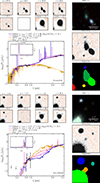 |
Fig. 15. Illustrative data for two galaxies observed by DAWN PL. See the main text for details. Top: Most massive galaxy from DAWN PL with a reliable spectroscopic redshift at z > 3, with log10(ℳ/M⊙) = 11.1 ± 0.1. The galaxy is located in EDF-F (which does not include HSC y imaging) and the reported ID corresponds to the DAWN PL EDF-F catalogue. The spectroscopic redshift is obtained from cross-matching to with GOODS-S catalogue (Garilli et al. 2021; Kodra et al. 2023). Bottom: Most massive galaxy observed at 4.5 < z ≤ 5.5. The stellar mass is highly uncertain at |
Another systematic bias may be introduced by the unaccounted for presence of AGNs. Using LePHARE, a set of AGN (or quasi-stellar object) templates are fit to every object alongside galaxy and stellar templates following Weaver et al. (2022, see also Laigle et al. 2016). There do not appear to be any massive galaxies that have SEDs that cannot be explained predominantly by stellar emission. However, it is difficult to observationally distinguish AGNs without MIR/FIR imaging, and therefore some of the best-fit AGN templates are degenerate with the galaxy solution. As pointed out by W23, it is not clear whether AGNs at z > 3 are bright enough in the rest-frame optical/NIR to significantly skew stellar mass measurements and resulting constraints on number densities. For example, the authors point to Ito et al. (2022), which showed that although AGNs appear common at these redshifts, their optical emission is more than an order of magnitude less than what is emitted in stellar light from their host galaxies. Recently, Guo et al. (2025) measured the abundance of AGNs at z ∼ 5 compared to ordinary galaxies and found that their abundance is between 0.5–1 dex smaller than Lyman break galaxies. As such, it is unlikely for a randomly selected galaxy to suffer severe AGN contamination.
The unaccounted for contribution of an AGN is likely to have a more significant effect at low redshifts. Using a sample of ∼900 X-ray luminous AGNs at 0.5 < z ≤ 3, Florez et al. (2020) showed that stellar mass estimates become increasingly overestimated with increasing fAGN, where fAGN is the fraction of emission from 8–1000 μm contributed by AGNs relative to stars. At fAGN > 0.6, stellar masses can be overestimated by up 0.5 dex (with some scatter). This result could significantly impact the massive end of the SMF if galaxies with very luminous AGNs are ubiquitous in massive galaxies. However, the authors compare the abundance of luminous AGNs to galaxies without X-ray counterparts and find that the latter are 2 orders of magnitude more abundant at log10(ℳ/M⊙) > 11. The abundance of luminous AGNs (or lack thereof) suggests their cumulative effect on the SMF is generally not substantial, despite the presence of an AGN in an individual system. Definitive quantification of this effect remains elusive even in richer multi-wavelength fields (cf. W23). Indeed, regardless of redshift, removing all galaxies that have smaller χ2 values in the best-fit AGN templates compared to the best-fit galaxy template has a negligible impact on the galaxy SMF.
Forrest et al. (2024a) show that the number density of massive galaxies, for example log10(ℳ/M⊙) > 11.5, can be overestimated at 3 < z < 4 due to the misclassification of very dusty galaxies at low z. Generally, their result likely has some applicability to the massive galaxies found here at 3 < z < 4, although the extent is unclear. In some cases, the P(z) measured by LePHARE shows two peaks, and a secondary photo-z solution can be inferred where the secondary solution is implies a low-redshift dusty galaxy. However, in detail, it is not immediately clear that the galaxies targeted by Forrest et al. (2024a) are detected in DAWN PL. First, the galaxies are selected from NIR imaging and photometry rather than from optical. More importantly, both their photometric- and spectroscopic-inferred rest-frame colours (e.g. Figs. 1 and 5 of Forrest et al. 2024a, respectively) indicate a parameter space that is precluded by DAWN PL’s optical selection function. The former partially overlap with the UVJ selection boundary for quiescent systems, while the latter shows that these galaxies are, in fact, extremely dusty. Although there are differences between the UVJ-selections and NUVrJ-selections (Sect. 3.2), there are virtually zero quiescent galaxy candidates found at z > 3 in DAWN PL, and even the ‘dusty’ quadrant of the NUVrJ diagram is essentially empty above z > 3. Consider further the comparison between this work, D17, and W23 at 3.0 < z ≤ 4.5 in Fig. 5 and Fig. 6. The excess of W23 over D17 and this work appears to be driven by galaxies that are faint and intrinsically redder than what can be detected from the HSC r + i + z selection. Consequently, it is possible that the interloper population identified by Forrest et al. (2024a) does not imply a drastic reduction in the number-densities of massive galaxies presented here.
6.4.2. Ultra-massive galaxies
This work introduces a hitherto unexplored region of parameter space occupied by ultra-massive galaxies. Seen only in smaller surveys by chance, their impact on the bright-end of the SMF can be enormous (see Sect. 5.4.1). This section presents some of the most convincing candidates yet found.
Figure 15 presents the most massive galaxy at z > 3 with a reliable spectroscopic confirmation, and the galaxy discussed in Sect. 6.2 with a stellar mass requiring and integrated star-formation efficiency ϵ > 1 at z ∼ 5. The first galaxy, shown in the upper panel of Fig. 15, is located in EDF-F with zspec = 3.08 (zphot = 3.07) and log10(ℳ/M⊙) = 11.1 ± 0.1. The spectroscopic redshift is obtained from the GOODS-S catalogue (Garilli et al. 2021; Kodra et al. 2023), which overlaps EDF-F. In addition to showcasing a resolved morphology and large physical size, the galaxy is characterised by a relatively flat SED and weak Balmer break. This galaxy is likely forming stars efficiently and may have a young stellar population; indeed, referring back to Fig. 12, this galaxy should be approximately at the peak of the SHMR. Galaxies at this redshift are easily disentangled from stellar interlopers, in particular based on their g − z and z − [3.6 μm] colours. Note that there is not any HSC y coverage over EDF-F, thus the blank cutout. Generally, this galaxy highlights the ability to properly identify galaxies known to be at high redshifts using the DAWN PL photometry, though EC-Z25 presents further detail regarding the performance of the DAWN PL photo-z in comparison to 3300 spectroscopic galaxies matched to the GOODS-S catalogue. Although there is no way to directly validate the stellar mass of this particular galaxy at present, EC-Z25 also provides a demonstration that shows that when the redshift of the galaxy is accurate, the resulting ℳ obtained from DAWN PL is fully consistent with what would be inferred from photometry including NIR (and additional) constraints.
The second galaxy, shown in the lower panel of Fig. 15 is located in EDF-N with zphot = 5.15 and  . The asymmetric uncertainty is indicative of the parameter space and the P(ℳ) for the galaxy: the probability distribution is broad but includes a local maximum near log10(ℳ/M⊙) = 12.5, with few models capable of producing greater stellar mass. The cutouts and reported magnitudes show that the galaxy is ∼4.5 magnitudes brighter in Spitzer/IRAC compared to HSC z, thus driving the substantial stellar mass. Stellar population ages in the galaxy templates are required to be younger than the age of the Universe at the assumed redshift, though such a significant excess beyond 4000 Å (rest frame) implies an advanced age, assuming the redshift is correct. The P(z) shows multiple peaks, and any lower value would lower the stellar mass while providing additional time to grow an old stellar population. The uncertainty in the stellar mass may be driven by an uncertainty in the dust content, which is not well constrained due to the lack of NIR photometry. In any case, the 4.5 magnitude difference between z and [3.6 μm] is extreme. Although no emission lines are included in the best-fit template, the secondary redshift solution includes emission lines expected for a star-forming galaxy. Again, it must be emphasised that the physical properties, including photo-z and ℳ, are not inferred from any one template but from the posterior distributions, consistent with D17 and W23. It is not expected that the foreground object visible in the lower left corner of the cutouts impacts the photometry of this galaxy, despite its proximity. The segmentation of the image looks reasonable, and Weaver et al. (2023b) provides several demonstrations of The Farmer photometry package that show that the light from objects in such proximity to one another can be properly distinguished. Moreover, the stellar mass is primarily driven by the [3.6 μm] and [4.5 μm] fluxes, which are significant and do not appear contaminated by the neighbouring object.
The degeneracy among the galaxy, AGN, and star templates is clearly evident in the second galaxy (right panel, Fig. 15). As discussed in Sect. 6.4.1, it is not clear whether an AGN at this redshift would be bright enough at the observed wavelengths to impact the stellar mass estimate, though a sizeable contribution from AGNs light would bring the ℳ estimate down. To reiterate the above, removing all galaxies that have smaller χ2 values in the best-fit AGN template compared to the best-fit galaxy template is inconsequential to the galaxy SMF, but doing so would have removed this source, which appears interesting and worthy of discussion. Comparing the χ2 values, the stellar template is rejected with high confidence, although visually it appears to be a reasonable fit. In the short-term, NIR observations from Euclid may provide clarity on the physical properties of this galaxy, and at least provide further confidence in ruling out the stellar solution. However, determining the true nature of this galaxy ultimately requires spectroscopic follow-up.
7. Summary and conclusions
We have characterised the evolution of the galaxy SMF across 0.2 < z ≤ 6.5 using the DAWN PL catalogues. The DAWN PL catalogues span an effective area of 10.13 deg2, exceeding COSMOS (Scoville et al. 2007; Weaver et al. 2022) and the recent analyses of the galaxy SMF therein of W23 by an order of magnitude and of Shuntov et al. (2025) by a factor of 20. Such a unique, tenfold increase in volume samples cosmologically diverse structure and environments while also exploring new parameter spaces of the most massive galaxies, which cannot be found in smaller surveys. This work constitutes a benchmark for the ‘pre-launch’ analysis of the galaxy SMF.
Generally, the abundance of massive systems observed by W23 is confirmed and upper limits of number density are replaced by firm estimates. A few dozen galaxy candidates are also observed with even greater stellar masses. This was enabled by a significant reduction in both Poisson uncertainty and cosmic variance (e.g. a factor of ∼5 for galaxies with ℳ ∼ 1011 M⊙ at z ∼ 5). All galaxies are detected from a deep composite stack of Subaru HSC r + i + z that rivals shallower NIR selection (e.g. D17) and reaches stellar masses above ℳ ∼ 1010 M⊙ at z ∼ 6. However, there is evidence that the most significantly dust-attenuated galaxies are not detected above z ∼ 1.5.
The number density of galaxies is described by a total uncertainty that includes Poisson uncertainty, cosmic variance, and uncertainty due to SED fitting with a zeroth-order correction for the covariance of stellar mass with redshift. To z ∼ 3, the SMF can be separated into a star-forming component and a quiescent component. A Schechter function, or a double Schechter function where appropriate, was used to infer the intrinsic total SMF as well as the star-forming and quiescent components, with Eddington bias accounted for following the procedure outlined in Ilbert et al. (2013), D17, and W23. The observed and intrinsic SMFs were compared to the most recent measurements in the COSMOS field as well as representative space-based measurements from HST and JWST (Grazian et al. 2015; Weibel et al. 2024); we find good agreement across all redshifts but with minor differences at z ∼ 5–6 caused by the selection functions. Selection function aside, the most significant difference with measurements from space-based facilities is the difference in volume explored: DAWN PL samples a volume between 70 and 100 times larger, and thus the improvements in Poisson uncertainty, cosmic variance, and access to massive galaxies over W23 are even greater compared to G15 and W24.
Additional key results of this analysis are as follows:
-
We compared the intrinsic and observed SMF with the Tinker et al. (2008) dark matter HMF at each redshift under various integrated star-formation efficiencies, ϵ. Up until z ∼ 3, the abundance relative to the HMF of galaxies with stellar masses above and below the characteristic stellar mass, ℳ★, is indicative of inefficient star formation (ϵ < 0.1). However, massive galaxies requiring ϵ > 0.3–0.5 are observed across 3.5 < z ≤ 6.5. Their abundance provides substantial evidence that feedback mechanisms in massive galaxies are not strong enough to regulate their star formation at this epoch or before, as suggested by recent numerical simulations (Valentini et al. 2021; Bassini et al. 2023) and recent measurements of the SHMR (Shuntov et al. 2022).
-
Exceptionally massive quiescent galaxies (ℳ > 1011.7 M⊙) are already fully formed as early as z ∼ 2.5 with a number density (Φ) of ∼10−6 Mpc−3. Their number density is consistent with little to no growth from z ∼ 2.5–3 to z ∼ 0.2, suggesting that their gas supplies are completely consumed or otherwise disrupted and that feedback mechanisms prevent further growth (Fiore et al. 2017). The inappreciable increase in their number density over time is consistent with the expected stellar mass growth from mergers in galaxies with ℳ > 1011 M⊙ across these redshifts (Mundy et al. 2017; Conselice et al. 2022) and appears to extend the result of Kawinwanichakij et al. (2020) to even earlier times for quiescent systems.
-
The galaxy SMF is investigated as a function of environment out to z ∼ 3.5 following a rudimentary characterisation of the density field based on Kovač et al. (2010). At 0.8 < z ≤ 1.1, the quiescent SMF in the most dense regions shows clear signs of ‘environmental quenching’ (Peng et al. 2010). In contrast to some previous works (e.g. Papovich et al. 2018), but supported by others (Davidzon et al. 2016; Tomczak et al. 2017), massive galaxies of all types are preferentially found in high-density environments at all redshifts. The environmental dependence appears weaker at earlier times; however, massive galaxies are observed to be more abundant in high-density environments as early as 3 < z ≤ 3.5, while less massive galaxies are preferentially located in low-density environments.
As emphasised above, DAWN PL has provided a powerful dataset uniquely suited to characterising the high-mass end of the galaxy SMF due to the exceptionally deep Spitzer/IRAC imaging over an unmatched area. Eventually, EDF-N and EDF-F (as well as EDF-S and the EAFs) will be observed by Euclid to NIR depths of 26 mag (Euclid Collaboration: McPartland et al. 2025; Euclid Collaboration: Mellier et al. 2025), providing an opportunity for a ‘post-launch’ analysis of the galaxy SMF. These data will be processed as part of the official Euclid data releases and matched with Spitzer/IRAC in future data releases from DAWN. Upon their releases, a window of exploration will be opened through the epoch of re-ionisation to at least z ∼ 8 with greater statistical power than this work and with further potential to discover intrinsically red massive galaxies. In addition, an improvement in the photo-z performance is expected from the NIR photometry, as well as a more complete selection of quiescent galaxies at z > 1.5 and robust rejection of interloper populations. Complementing the imminent NIR photometry, Euclid will also obtain hundreds of thousands of spectroscopic redshifts in the EDFs and EAFs alone (Euclid Collaboration: Mellier et al. 2025), enabling a precise characterisation of the clustering of galaxies and therefore the connection to both their dark matter halos and their local environments The combination of the survey area, wavelength coverage, photometric depth, and complementary spectroscopy will establish a legacy of precision galaxy demographics and galaxy evolution studies that push ever further into the cosmic past.
Data availability
FITS files are available at the CDS via anonymous ftp to https://cdsarc.cds.unistra.fr/viz-bin/cat/J/A+A/708/A104
Acknowledgments
J.R.W. acknowledges that support for this work was provided by The Brinson Foundation through a Brinson Prize Fellowship grant. The Euclid Consortium acknowledges the European Space Agency and a number of agencies and institutes that have supported the development of Euclid, in particular the Agenzia Spaziale Italiana, the Austrian Forschungsförderungsgesellschaft funded through BMIMI, the Belgian Science Policy, the Canadian Euclid Consortium, the Deutsches Zentrum für Luft- und Raumfahrt, the DTU Space and the Niels Bohr Institute in Denmark, the French Centre National d’Etudes Spatiales, the Fundação para a Ciência e a Tecnologia, the Hungarian Academy of Sciences, the Ministerio de Ciencia, Innovación y Universidades, the National Aeronautics and Space Administration, the National Astronomical Observatory of Japan, the Netherlandse Onderzoekschool Voor Astronomie, the Norwegian Space Agency, the Research Council of Finland, the Romanian Space Agency, the Swiss Space Office (SSO) at the State Secretariat for Education, Research, and Innovation (SERI), and the United Kingdom Space Agency. A complete and detailed list is available on the Euclid web site (www.euclid-ec.org/consortium/community/).
References
- Adams, N. J., Bowler, R. A. A., Jarvis, M. J., Häußler, B., & Lagos, C. D. P. 2021, MNRAS, 506, 4933 [CrossRef] [Google Scholar]
- Agertz, O., Kravtsov, A. V., Leitner, S. N., & Gnedin, N. Y. 2013, ApJ, 770, 25 [NASA ADS] [CrossRef] [Google Scholar]
- Arnouts, S., Moscardini, L., Vanzella, E., et al. 2002, MNRAS, 329, 355 [Google Scholar]
- Arnouts, S., Walcher, C. J., Le Fèvre, O., et al. 2007, A&A, 476, 137 [CrossRef] [EDP Sciences] [Google Scholar]
- Ashby, M. L. N., Caputi, K. I., Cowley, W., et al. 2018, ApJS, 237, 39 [CrossRef] [Google Scholar]
- Bahcall, N. A., & Cen, R. 1993, ApJ, 407, L49 [NASA ADS] [CrossRef] [Google Scholar]
- Barbary, K. 2016, J. Open Source Software, 1, 58 [NASA ADS] [CrossRef] [Google Scholar]
- Bassini, L., Feldmann, R., Gensior, J., et al. 2023, MNRAS, 525, 5388 [NASA ADS] [CrossRef] [Google Scholar]
- Beck, R., McPartland, C., Repp, A., et al. 2020, MNRAS, 493, 2318 [NASA ADS] [CrossRef] [Google Scholar]
- Beckmann, R. S., Devriendt, J., Slyz, A., et al. 2017, MNRAS, 472, 949 [NASA ADS] [CrossRef] [Google Scholar]
- Behroozi, P., & Silk, J. 2018, MNRAS, 477, 5382 [Google Scholar]
- Behroozi, P. S., Wechsler, R. H., & Conroy, C. 2013, ApJ, 770, 57 [NASA ADS] [CrossRef] [Google Scholar]
- Behroozi, P., Wechsler, R. H., Hearin, A. P., & Conroy, C. 2019, MNRAS, 488, 3143 [NASA ADS] [CrossRef] [Google Scholar]
- Bertin, E. 2010, Astrophysics Source Code Library [record ascl:1010.068] [Google Scholar]
- Bertin, E., Mellier, Y., Radovich, M., et al. 2002, ASP Conf. Ser., 281, 228 [Google Scholar]
- Bhatawdekar, R., Conselice, C. J., Margalef-Bentabol, B., & Duncan, K. 2019, MNRAS, 486, 3805 [NASA ADS] [CrossRef] [Google Scholar]
- Bolzonella, M., Kovac, K., Pozzetti, L., et al. 2010, A&A, 524, A76 [NASA ADS] [CrossRef] [EDP Sciences] [Google Scholar]
- Boulade, O., Charlot, X., Abbon, P., et al. 2003, SPIE Conf. Ser., 4841, 72 [Google Scholar]
- Bower, R. G., Benson, A. J., Malbon, R., et al. 2006, MNRAS, 370, 645 [Google Scholar]
- Boylan-Kolchin, M. 2023, Nat. Astron., 7, 731 [NASA ADS] [CrossRef] [Google Scholar]
- Boylan-Kolchin, M., Springel, V., White, S. D. M., Jenkins, A., & Lemson, G. 2009, MNRAS, 398, 1150 [Google Scholar]
- Brammer, G. B., van Dokkum, P. G., & Coppi, P. 2008, ApJ, 686, 1503 [Google Scholar]
- Breiman, L. 2001, Mach. Learn., 45, 5 [Google Scholar]
- Brinchmann, J., Charlot, S., White, S. D. M., et al. 2004, MNRAS, 351, 1151 [Google Scholar]
- Bundy, K., Ellis, R. S., Conselice, C. J., et al. 2006, ApJ, 651, 120 [Google Scholar]
- Capak, P., Arendt, R., Arnouts, S., et al. 2016, The Euclid/WFIRST Spitzer Legacy Survey, Spitzer Proposal [Google Scholar]
- Capozzi, D., Etherington, J., Thomas, D., et al. 2017, arXiv e-prints [arXiv:1707.09066] [Google Scholar]
- Caputi, K. I., Cirasuolo, M., Dunlop, J. S., et al. 2011, MNRAS, 413, 162 [NASA ADS] [CrossRef] [Google Scholar]
- Caputi, K. I., Ilbert, O., Laigle, C., et al. 2015, ApJ, 810, 73 [Google Scholar]
- Casey, C. M., Akins, H. B., Shuntov, M., et al. 2024, ApJ, 965, 98 [NASA ADS] [CrossRef] [Google Scholar]
- Chabrier, G. 2003, PASP, 115, 763 [Google Scholar]
- Chartab, N., Mobasher, B., Cooray, A. R., et al. 2023, ApJ, 942, 91 [Google Scholar]
- Chary, R.-R. 2008, ApJ, 680, 32 [Google Scholar]
- Chen, Y., Mo, H. J., & Wang, K. 2023, MNRAS, 526, 2542 [Google Scholar]
- Chuang, C.-Y., Jespersen, C. K., Lin, Y.-T., Ho, S., & Genel, S. 2024, ApJ, 965, 101 [Google Scholar]
- Clerc, N., Adami, C., Lieu, M., et al. 2014, MNRAS, 444, 2723 [NASA ADS] [CrossRef] [Google Scholar]
- Conroy, C. 2013, ARA&A, 51, 393 [NASA ADS] [CrossRef] [Google Scholar]
- Conselice, C. J. 2014, ARA&A, 52, 291 [CrossRef] [Google Scholar]
- Conselice, C. J., Mundy, C. J., Ferreira, L., & Duncan, K. 2022, ApJ, 940, 168 [CrossRef] [Google Scholar]
- Contreras, S., Baugh, C. M., Norberg, P., & Padilla, N. 2015, MNRAS, 452, 1861 [CrossRef] [Google Scholar]
- Cowie, L. L., Songaila, A., Hu, E. M., & Cohen, J. G. 1996, AJ, 112, 839 [Google Scholar]
- Croton, D. J. 2013, PASA, 30, e052 [NASA ADS] [CrossRef] [Google Scholar]
- Cucciati, O., Tresse, L., Ilbert, O., et al. 2012, A&A, 539, A31 [NASA ADS] [CrossRef] [EDP Sciences] [Google Scholar]
- Daddi, E., Dickinson, M., Morrison, G., et al. 2007, ApJ, 670, 156 [NASA ADS] [CrossRef] [Google Scholar]
- Dark Energy Survey Collaboration (Abbott, T., et al.) 2016, MNRAS, 460, 1270 [Google Scholar]
- Davidzon, I., Cucciati, O., Bolzonella, M., et al. 2016, A&A, 586, A23 [NASA ADS] [CrossRef] [EDP Sciences] [Google Scholar]
- Davidzon, I., Ilbert, O., Laigle, C., et al. 2017, A&A, 605, A70 [NASA ADS] [CrossRef] [EDP Sciences] [Google Scholar]
- Davis, M., Guhathakurta, P., Konidaris, N. P., et al. 2007, ApJ, 660, L1 [NASA ADS] [CrossRef] [Google Scholar]
- Dekel, A., Birnboim, Y., Engel, G., et al. 2009, Nature, 457, 451 [Google Scholar]
- Dekel, A., Sarkar, K. C., Birnboim, Y., Mandelker, N., & Li, Z. 2023, MNRAS, 523, 3201 [NASA ADS] [CrossRef] [Google Scholar]
- Duncan, K., Conselice, C. J., Mortlock, A., et al. 2014, MNRAS, 444, 2960 [Google Scholar]
- Dunne, L., Ivison, R. J., Maddox, S., et al. 2009, MNRAS, 394, 3 [NASA ADS] [CrossRef] [Google Scholar]
- Ebeling, H. 2004, MNRAS, 349, 768 [Google Scholar]
- Eddington, A. S. 1913, MNRAS, 73, 359 [Google Scholar]
- Eddington, A. S. 1940, MNRAS, 100, 354 [Google Scholar]
- Edward, A. H., Balogh, M. L., Bahé, Y. M., Cooper, M. C., et al. 2024, MNRAS, 527, 8598 [Google Scholar]
- Elbaz, D., Daddi, E., Le Borgne, D., et al. 2007, A&A, 468, 33 [NASA ADS] [CrossRef] [EDP Sciences] [Google Scholar]
- Etherington, J., Thomas, D., Maraston, C., et al. 2016, MNRAS, 466, 228 [Google Scholar]
- Euclid Collaboration (Moneti, A., et al.) 2022, A&A, 658, A126 [NASA ADS] [CrossRef] [EDP Sciences] [Google Scholar]
- Euclid Collaboration (Scaramella, R., et al.) 2022, A&A, 662, A112 [NASA ADS] [CrossRef] [EDP Sciences] [Google Scholar]
- Euclid Collaboration (McPartland, C. J. R., et al.) 2025, A&A, 695, A259 [Google Scholar]
- Euclid Collaboration (Mellier, Y., et al.) 2025, A&A, 697, A1 [Google Scholar]
- Euclid Collaboration (Zalesky, L., et al.) 2025, A&A, 695, A229 [Google Scholar]
- Fabian, A. C. 2012, ARA&A, 50, 455 [Google Scholar]
- Fiore, F., Feruglio, C., Shankar, F., et al. 2017, A&A, 601, A143 [NASA ADS] [CrossRef] [EDP Sciences] [Google Scholar]
- Florez, J., Jogee, S., Sherman, S., et al. 2020, MNRAS, 497, 3273 [NASA ADS] [CrossRef] [Google Scholar]
- Foreman-Mackey, D., Hogg, D. W., Lang, D., & Goodman, J. 2013, PASP, 125, 306 [Google Scholar]
- Forrest, B., Cooper, M. C., Muzzin, A., et al. 2024a, ApJ, 977, 51 [Google Scholar]
- Forrest, B., Lemaux, B. C., Shah, E. A., et al. 2024b, ApJ, 971, 169 [NASA ADS] [Google Scholar]
- Förster Schreiber, N. M., & Wuyts, S. 2020, ARA&A, 58, 661 [Google Scholar]
- Fujimoto, S., Ouchi, M., Ferrara, A., et al. 2019, ApJ, 887, 107 [Google Scholar]
- Furtak, L. J., Atek, H., Lehnert, M. D., Chevallard, J., & Charlot, S. 2021, MNRAS, 501, 1568 [Google Scholar]
- Gaia Collaboration (Vallenari, A., et al.) 2023, A&A, 674, A1 [NASA ADS] [CrossRef] [EDP Sciences] [Google Scholar]
- Garilli, B., McLure, R., Pentericci, L., et al. 2021, A&A, 647, A150 [NASA ADS] [CrossRef] [EDP Sciences] [Google Scholar]
- Gehrels, N. 1986, ApJ, 303, 336 [Google Scholar]
- Giavalisco, M., Ferguson, H. C., Koekemoer, A. M., et al. 2004, ApJ, 600, L93 [NASA ADS] [CrossRef] [Google Scholar]
- Gómez, P. L., Nichol, R. C., Miller, C. J., et al. 2003, ApJ, 584, 210 [Google Scholar]
- González, V., Labbé, I., Bouwens, R. J., et al. 2011, ApJ, 735, L34 [Google Scholar]
- Grazian, A., Fontana, A., Santini, P., et al. 2015, A&A, 575, A96 [NASA ADS] [CrossRef] [EDP Sciences] [Google Scholar]
- Gruppioni, C., Pozzi, F., Rodighiero, G., et al. 2013, MNRAS, 432, 23 [Google Scholar]
- Guo, Q., White, S., Boylan-Kolchin, M., et al. 2011, MNRAS, 413, 101 [Google Scholar]
- Guo, J., Onoue, M., Inayoshi, K., Kocevski, D. D., et al. 2025, ApJ, 991, 74 [Google Scholar]
- Guzzo, L., Scodeggio, M., Garilli, B., et al. 2014, A&A, 566, A108 [NASA ADS] [CrossRef] [EDP Sciences] [Google Scholar]
- Harikane, Y., Ouchi, M., Ono, Y., et al. 2018, PASJ, 70, S11 [NASA ADS] [CrossRef] [Google Scholar]
- Harikane, Y., Ouchi, M., Oguri, M., et al. 2023, ApJS, 265, 5 [NASA ADS] [CrossRef] [Google Scholar]
- Harvey, T., Conselice, C. J., Adams, N. J., et al. 2025, ApJ, 978, 89 [NASA ADS] [CrossRef] [Google Scholar]
- Henriques, B. M. B., White, S. D. M., Thomas, P. A., et al. 2015, MNRAS, 451, 2663 [Google Scholar]
- Hildebrandt, H., Erben, T., Kuijken, K., et al. 2012, MNRAS, 421, 2355 [Google Scholar]
- Hogg, D. W., Baldry, I. K., Blanton, M. R., & Eisenstein, D. J. 2002, arXiv e-prints [arXiv:astro-ph/0210394] [Google Scholar]
- Hopkins, P. F., Quataert, E., & Murray, N. 2012, MNRAS, 421, 3522 [Google Scholar]
- Hopkins, P. F., Kereš, D., Oñorbe, J., et al. 2014, MNRAS, 445, 581 [NASA ADS] [CrossRef] [Google Scholar]
- Hopkins, P. F., Wetzel, A., Kereš, D., et al. 2018, MNRAS, 480, 800 [NASA ADS] [CrossRef] [Google Scholar]
- Hung, D., Lemaux, B. C., Gal, R. R., et al. 2021, MNRAS, 502, 3942 [NASA ADS] [CrossRef] [Google Scholar]
- Ilbert, O., Tresse, L., Zucca, E., et al. 2005, A&A, 439, 863 [NASA ADS] [CrossRef] [EDP Sciences] [Google Scholar]
- Ilbert, O., Arnouts, S., McCracken, H. J., et al. 2006, A&A, 457, 841 [NASA ADS] [CrossRef] [EDP Sciences] [Google Scholar]
- Ilbert, O., Salvato, M., Le Floc’h, E., et al. 2010, ApJ, 709, 644 [Google Scholar]
- Ilbert, O., McCracken, H. J., Le Fèvre, O., et al. 2013, A&A, 556, A55 [NASA ADS] [CrossRef] [EDP Sciences] [Google Scholar]
- Ito, K., Tanaka, M., Miyaji, T., et al. 2022, ApJ, 929, 53 [NASA ADS] [CrossRef] [Google Scholar]
- Ivezić, Ž., Kahn, S. M., Tyson, J. A., et al. 2019, ApJ, 873, 111 [Google Scholar]
- Jespersen, C. K., Cranmer, M., Melchior, P., et al. 2022, ApJ, 941, 7 [NASA ADS] [CrossRef] [Google Scholar]
- Jespersen, C. K., Steinhardt, C. L., Somerville, R. S., & Lovell, C. C. 2025, ApJ, 982, 23 [Google Scholar]
- Kauffmann, G., White, S. D. M., Heckman, T. M., et al. 2004, MNRAS, 353, 713 [Google Scholar]
- Kawinwanichakij, L., Papovich, C., Quadri, R. F., et al. 2017, ApJ, 847, 134 [NASA ADS] [CrossRef] [Google Scholar]
- Kawinwanichakij, L., Papovich, C., Ciardullo, R., et al. 2020, ApJ, 892, 7 [Google Scholar]
- Kikuchihara, S., Ouchi, M., Ono, Y., et al. 2020, ApJ, 893, 60 [NASA ADS] [CrossRef] [Google Scholar]
- Kistler, M. D., Yuksel, H., & Hopkins, A. M. 2013, arXiv e-prints [arXiv:1305.1630] [Google Scholar]
- Kodra, D., Andrews, B. H., Newman, J. A., et al. 2023, ApJ, 942, 36 [NASA ADS] [CrossRef] [Google Scholar]
- Kovač, K., Lilly, S. J., Cucciati, O., et al. 2010, ApJ, 708, 505 [CrossRef] [Google Scholar]
- Laigle, C., McCracken, H. J., Ilbert, O., et al. 2016, ApJS, 224, 24 [Google Scholar]
- Lang, D., Hogg, D. W., & Mykytyn, D. 2016, Astrophysics Source Code Library [record ascl:1604.008] [Google Scholar]
- Laureijs, R., Amiaux, J., Arduini, S., et al. 2011, arXiv e-prints [arXiv:1110.3193] [Google Scholar]
- Le Borgne, D., Elbaz, D., Ocvirk, P., & Pichon, C. 2009, A&A, 504, 727 [NASA ADS] [CrossRef] [EDP Sciences] [Google Scholar]
- Leja, J., Tacchella, S., & Conroy, C. 2019, ApJ, 880, L9 [NASA ADS] [CrossRef] [Google Scholar]
- Li, Z., Dekel, A., Sarkar, K. C., et al. 2024, A&A, 690, A108 [NASA ADS] [CrossRef] [EDP Sciences] [Google Scholar]
- Lilly, S. J., Le Fèvre, O., Renzini, A., et al. 2007, ApJS, 172, 70 [Google Scholar]
- Lotz, J. M., Jonsson, P., Cox, T. J., & Primack, J. R. 2010, MNRAS, 404, 575 [Google Scholar]
- Lubin, L. M., Gal, R. R., Lemaux, B. C., Kocevski, D. D., & Squires, G. K. 2009, AJ, 137, 4867 [Google Scholar]
- Madau, P., & Dickinson, M. 2014, ARA&A, 52, 415 [Google Scholar]
- Malmquist, K. G. 1922, Meddelanden fran Lunds Astronomiska Observatorium Serie I, 100, 1 [Google Scholar]
- Malmquist, K. G. 1925, Meddelanden fran Lunds Astronomiska Observatorium Serie I, 106, 1 [Google Scholar]
- Man, Z.-Y., Peng, Y.-J., Shi, J.-J., et al. 2019, ApJ, 881, 74 [Google Scholar]
- Marchesini, D., van Dokkum, P. G., Förster Schreiber, N. M., et al. 2009, ApJ, 701, 1765 [NASA ADS] [CrossRef] [Google Scholar]
- Marinoni, C., & Hudson, M. J. 2002, ApJ, 569, 101 [NASA ADS] [CrossRef] [Google Scholar]
- Martin, D. C., Wyder, T. K., Schiminovich, D., et al. 2007, ApJS, 173, 342 [NASA ADS] [CrossRef] [Google Scholar]
- McCracken, H. J., Milvang-Jensen, B., Dunlop, J., et al. 2012, A&A, 544, A156 [NASA ADS] [CrossRef] [EDP Sciences] [Google Scholar]
- McLeod, D. J., McLure, R. J., Dunlop, J. S., et al. 2021, MNRAS, 503, 4413 [NASA ADS] [CrossRef] [Google Scholar]
- Metuki, O., Libeskind, N. I., Hoffman, Y., Crain, R. A., & Theuns, T. 2015, MNRAS, 446, 1458 [NASA ADS] [CrossRef] [Google Scholar]
- Mitchell, P. D., Lacey, C. G., Baugh, C. M., & Cole, S. 2013, MNRAS, 435, 87 [NASA ADS] [CrossRef] [Google Scholar]
- Miyazaki, S., Komiyama, Y., Kawanomoto, S., et al. 2018, PASJ, 70, S1 [NASA ADS] [Google Scholar]
- Mobasher, B., Dahlen, T., Ferguson, H. C., et al. 2015, ApJ, 808, 101 [NASA ADS] [CrossRef] [Google Scholar]
- Moster, B. P., Somerville, R. S., Maulbetsch, C., et al. 2010, ApJ, 710, 903 [Google Scholar]
- Moster, B. P., Somerville, R. S., Newman, J. A., & Rix, H.-W. 2011, ApJ, 731, 113 [Google Scholar]
- Mundy, C. J., Conselice, C. J., Duncan, K. J., et al. 2017, MNRAS, 470, 3507 [Google Scholar]
- Muzzin, A., Marchesini, D., Stefanon, M., et al. 2013, ApJ, 777, 18 [NASA ADS] [CrossRef] [Google Scholar]
- Noeske, K. G., Weiner, B. J., Faber, S. M., et al. 2007, ApJ, 660, L43 [CrossRef] [Google Scholar]
- Oemler, A. J. 1974, ApJ, 194, 1 [NASA ADS] [CrossRef] [Google Scholar]
- Oi, N., Goto, T., Matsuhara, H., et al. 2021, MNRAS, 500, 5024 [Google Scholar]
- Oke, J. B. 1974, ApJS, 27, 21 [Google Scholar]
- Pacifici, C., Iyer, K. G., Mobasher, B., et al. 2023, ApJ, 944, 141 [NASA ADS] [CrossRef] [Google Scholar]
- Papovich, C., Kawinwanichakij, L., Quadri, R. F., et al. 2018, ApJ, 854, 30 [NASA ADS] [CrossRef] [Google Scholar]
- Pearson, W. J., Wang, L., Alpaslan, M., et al. 2019, A&A, 631, A51 [NASA ADS] [CrossRef] [EDP Sciences] [Google Scholar]
- Peng, Y.-J., Lilly, S. J., Kovač, K., et al. 2010, ApJ, 721, 193 [Google Scholar]
- Peng, Y.-J., Lilly, S. J., Renzini, A., & Carollo, M. 2012, ApJ, 757, 4 [NASA ADS] [CrossRef] [Google Scholar]
- Popesso, P., Concas, A., Cresci, G., et al. 2023, MNRAS, 519, 1526 [Google Scholar]
- Porqueres, N., Jasche, J., Lavaux, G., & Enßlin, T. 2019, A&A, 630, A151 [NASA ADS] [CrossRef] [EDP Sciences] [Google Scholar]
- Pozzetti, L., Bolzonella, M., Zucca, E., et al. 2010, A&A, 523, A13 [NASA ADS] [CrossRef] [EDP Sciences] [Google Scholar]
- Riaz, R., Schleicher, D. R. G., Vanaverbeke, S., & Klessen, R. S. 2021, Astron. Nachr., 342, 157 [Google Scholar]
- Salim, S., Rich, R. M., Charlot, S., et al. 2007, ApJS, 173, 267 [NASA ADS] [CrossRef] [Google Scholar]
- Salpeter, E. E. 1955, ApJ, 121, 161 [Google Scholar]
- Santini, P., Fontana, A., Grazian, A., et al. 2012, A&A, 538, A33 [NASA ADS] [CrossRef] [EDP Sciences] [Google Scholar]
- Sawicki, M., Arnouts, S., Huang, J., et al. 2019, MNRAS, 489, 5202 [NASA ADS] [Google Scholar]
- Schaye, J., Crain, R. A., Bower, R. G., et al. 2015, MNRAS, 446, 521 [Google Scholar]
- Schaye, J., Kugel, R., Schaller, M., et al. 2023, MNRAS, 526, 4978 [NASA ADS] [CrossRef] [Google Scholar]
- Schechter, P. 1976, ApJ, 203, 297 [Google Scholar]
- Schmidt, M. 1968, ApJ, 151, 393 [Google Scholar]
- Scoville, N. Z. 2013, in Secular Evolution of Galaxies, eds. J. Falcón-Barroso, & J. H. Knapen, 491 [Google Scholar]
- Scoville, N., Aussel, H., Brusa, M., et al. 2007, ApJS, 172, 1 [Google Scholar]
- Shuntov, M., McCracken, H. J., Gavazzi, R., et al. 2022, A&A, 664, A61 [NASA ADS] [CrossRef] [EDP Sciences] [Google Scholar]
- Shuntov, M., Ilbert, O., Toft, S., et al. 2025, A&A, 695, A20 [NASA ADS] [CrossRef] [EDP Sciences] [Google Scholar]
- Silk, J., & Rees, M. J. 1998, A&A, 331, L1 [NASA ADS] [Google Scholar]
- Silk, J., Begelman, M. C., Norman, C., Nusser, A., & Wyse, R. F. G. 2024, ApJ, 961, L39 [NASA ADS] [CrossRef] [Google Scholar]
- Speagle, J. S., Steinhardt, C. L., Capak, P. L., & Silverman, J. D. 2014, ApJS, 214, 15 [Google Scholar]
- Springel, V., White, S. D. M., Jenkins, A., et al. 2005, Nature, 435, 629 [Google Scholar]
- Springel, V., Frenk, C. S., & White, S. D. M. 2006, Nature, 440, 1137 [NASA ADS] [CrossRef] [Google Scholar]
- Stanway, E. R., Bremer, M. N., Squitieri, V., Douglas, L. S., & Lehnert, M. D. 2008, MNRAS, 386, 370 [Google Scholar]
- Stark, D. P., Ellis, R. S., Bunker, A., et al. 2009, ApJ, 697, 1493 [NASA ADS] [CrossRef] [Google Scholar]
- Stefanon, M., Bouwens, R. J., Labbé, I., et al. 2021, ApJ, 922, 29 [NASA ADS] [CrossRef] [Google Scholar]
- Steinhardt, C. L., Capak, P., Masters, D., & Speagle, J. S. 2016, ApJ, 824, 21 [NASA ADS] [CrossRef] [Google Scholar]
- Steinhardt, C. L., Jespersen, C. K., & Linzer, N. B. 2021, ApJ, 923, 8 [NASA ADS] [CrossRef] [Google Scholar]
- Steinhardt, C. L., Sneppen, A., Mostafa, B., et al. 2022, ApJ, 931, 58 [NASA ADS] [CrossRef] [Google Scholar]
- Straatman, C. M. S., Spitler, L. R., Quadri, R. F., et al. 2016, ApJ, 830, 51 [NASA ADS] [CrossRef] [Google Scholar]
- Szalay, A. S., Connolly, A. J., & Szokoly, G. P. 1999, AJ, 117, 68 [Google Scholar]
- Taamoli, S., Mobasher, B., Chartab, N., et al. 2024, ApJ, 966, 18 [NASA ADS] [CrossRef] [Google Scholar]
- Tacconi, L. J., Genzel, R., & Sternberg, A. 2020, ARA&A, 58, 157 [NASA ADS] [CrossRef] [Google Scholar]
- Taylor, A. J., Barger, A. J., Cowie, L. L., et al. 2023, ApJS, 266, 24 [Google Scholar]
- Teerikorpi, P. 2004, A&A, 424, 73 [NASA ADS] [CrossRef] [EDP Sciences] [Google Scholar]
- Thorne, J. E., Robotham, A. S. G., Davies, L. J. M., et al. 2021, MNRAS, 505, 540 [NASA ADS] [CrossRef] [Google Scholar]
- Tinker, J., Kravtsov, A. V., Klypin, A., et al. 2008, ApJ, 688, 709 [Google Scholar]
- Tomczak, A. R., Quadri, R. F., Tran, K.-V. H., et al. 2014, ApJ, 783, 85 [Google Scholar]
- Tomczak, A. R., Lemaux, B. C., Lubin, L. M., et al. 2017, MNRAS, 472, 3512 [NASA ADS] [CrossRef] [Google Scholar]
- Valentini, M., Gallerani, S., & Ferrara, A. 2021, MNRAS, 507, 1 [NASA ADS] [CrossRef] [Google Scholar]
- van der Wel, A., Franx, M., van Dokkum, P. G., et al. 2014, ApJ, 788, 28 [Google Scholar]
- Vogelsberger, M., Genel, S., Sijacki, D., et al. 2013, MNRAS, 436, 3031 [Google Scholar]
- Vogelsberger, M., Genel, S., Springel, V., et al. 2014, Nature, 509, 177 [Google Scholar]
- Wang, T., Sun, H., Zhou, L., et al. 2025, ApJ, 988, L35 [Google Scholar]
- Weaver, J. R., Kauffmann, O. B., Ilbert, O., et al. 2022, ApJS, 258, 11 [NASA ADS] [CrossRef] [Google Scholar]
- Weaver, J. R., Davidzon, I., Toft, S., et al. 2023a, A&A, 677, A184 [NASA ADS] [CrossRef] [EDP Sciences] [Google Scholar]
- Weaver, J. R., Zalesky, L., Kokorev, V., et al. 2023b, ApJS, 269, 20 [NASA ADS] [CrossRef] [Google Scholar]
- Wechsler, R. H., & Tinker, J. L. 2018, ARA&A, 56, 435 [NASA ADS] [CrossRef] [Google Scholar]
- Weibel, A., Oesch, P. A., Barrufet, L., et al. 2024, MNRAS, 533, 1808 [NASA ADS] [CrossRef] [Google Scholar]
- Weigel, A. K., Schawinski, K., & Bruderer, C. 2016, MNRAS, 459, 2150 [NASA ADS] [CrossRef] [Google Scholar]
- Whitaker, K. E., Labbé, I., van Dokkum, P. G., et al. 2011, ApJ, 735, 86 [Google Scholar]
- Whitaker, K. E., van Dokkum, P. G., Brammer, G., et al. 2012, ApJ, 754, L29 [NASA ADS] [CrossRef] [Google Scholar]
- Williams, R. J., Quadri, R. F., Franx, M., van Dokkum, P., & Labbé, I. 2009, ApJ, 691, 1879 [NASA ADS] [CrossRef] [Google Scholar]
- Wright, A. H., Driver, S. P., & Robotham, A. S. G. 2018, MNRAS, 480, 3491 [Google Scholar]
- Wu, J. F., & Kragh Jespersen, C. 2023, arXiv e-prints [arXiv:2306.12327] [Google Scholar]
- Wu, J. F., Jespersen, C. K., & Wechsler, R. H. 2024, ApJ, 976, 37 [Google Scholar]
- Zitrin, A., Broadhurst, T., Bartelmann, M., et al. 2012, MNRAS, 423, 2308 [NASA ADS] [CrossRef] [Google Scholar]
Data files containing key observed measurements are available for download: https://zenodo.org/records/17634521.
Future releases from the DAWN survey will be detected from Euclid NIR imaging.
This is important since the highly skewed number count distributions in the limit of high cosmic variance bias the estimates of the cosmic variance, artificially inflating them.
Utilising a computing facility with 200 total cores and over 500 Gb of RAM, performing an MCMC simulation for 100 DAWN survey PL catalogues would require 1–2 years.
Note that at z ≥ 0.8, a single Schechter function is assumed, and the meaning of α1 changes.
Appendix A: Schechter parameters
Schechter parameters resulting from the MCMC analysis are presented in Table A.1 for the total sample, Table A.2 for the star-forming sample, and Table A.3 for the quiescent sample. The median of the marginalised posterior distributions of each parameter are shown with uncertainties corresponding to the 16th and 84th percentiles (i.e. enclosing 68% of the data). The maximum a posteriori parameter values are provided in brackets. Below, the comparison with the Schechter parameters of G15, D17, W23, and W24 is discussed.
Double (z ≤ 2) and single (z > 2) Schechter parameters derived for the total mass-complete sample.
Double (z ≤ 2) and single (z > 2) Schechter parameters derived for the star-forming mass-complete subsample.
Double (z ≤ 0.8) and single (z > 0.8) Schechter parameters derived for the quiescent mass-complete subsample.
Starting with the low-mass slope, the maximum a posteriori value and the median of the posterior are each consistent with the one or more of G15, D17, W23, or W24, by construction, i.e. due to the priors that are assumed. As a whole, the representative values of the low-mass slope are most similar to D17. To compare the other Schechter parameters with the literature, it must be acknowledged that the treatment of the Eddington bias between this work and other works may be different, which will affect the inferred values of the Schechter parameters.
Of particular interest in the literature is the appropriate value of the characteristic mass, ℳ★, at each redshift. The value of ℳ★ is believed to coincide with the peak of the SHMR and thus represents that stellar mass at which a galaxy is most efficient at converting baryons into stars (Behroozi et al. 2013; Wechsler & Tinker 2018). Following similar lines of reasoning, it is thought that above ℳ★, quenching mechanisms become more effective. The values of ℳ★ found here appear to be mostly consistent with the literature within the reported uncertainties, and especially with W23, the next largest survey by volume. Indeed, every value of ℳ★ through to and including 1.1 < z ≤ 1.5 is fully consistent with W23. Note that 1.1 < z ≤ 1.5 marks the onset of the increased uncertainty in photo-zs that leads to an excess of massive galaxies in DAWN PL. Nonetheless, median of the ℳ★ posterior distribution is  , while W23 reports a value of
  . This comparison, may suggest that the adopted Eddington bias kernel is reasonable given the resulting representative values of ℳ★. Although the representative values at 1.5 < z ≤ 2.0 and 2.0 < z ≤ 2.5 are somewhat larger than what was found by W23, they are very nearly consistent within 1σ. At 2.5 < z ≤ 3.0, where it is believed that the uncertainty in the photo-zs decreases is due to the Lyman break being better constrained, the representative value of ℳ★ is again fully consistent with W23 with a difference significantly less than the 1σ uncertainties.
As previously discussed, W23 fixes the value of the low-mass slope α at −1.46 at z > 2.5, while in this work the value of α is modelled with a prior that encourages a steeper (more negative) slope with increasing z. This is important to consider because α and ℳ★ are anti-correlated, with more negative (i.e. steeper) values of α leading to greater values of ℳ★ (see, again, Fig. 8 of Stefanon et al. 2021 and Fig. 7 of W24). As such, the representative values of ℳ★ should be generally greater than what was found by W23 at z ≫ 2.5 and they should agree more closely with works that found greater values of α at these redshifts (Grazian et al. 2015; Davidzon et al. 2017; Weibel et al. 2024). The former is confirmed throughout all remaining redshift bins. As for the latter, the representative value of ℳ★ is greater than what is found by D17 at 3.0 < z ≤ 3.5 but consistent within the reported 1σ uncertainties. The lowest-redshift bin of G15 and W24 is 3.5 < z ≤ 4.5. At these redshift, D17 notably reports a value of ℳ★ that increases significantly. The representative value of ℳ★ found in this work is lower than each of G15, W24, and D17, but remains consistent within their reported uncertainties. Looking more closely, the difference with D17 may be explained by their lower normalisation, where the two parameters are anti-correlated. Both G15 and W24 finds a higher value of ℳ★, while finding a smaller value for α. The comparison with G15 is sensible, as they report a much lower normalisation than either this work or W24. By contrast, W24 finds a similar normalisation to this work, and the source of the disagreement in the reported values of ℳ★ is not clear. At z ∼ 4, they assume an Gaussian-shaped Eddington bias kernel during their modelling with σ = 0.13, which has a similar overall shape to the kernel used herein (Eq. 11 with τc = 0.05 and σEdd = 0.6) but lacks the wings, which may be the cause.
At 4.5 < z ≤ 5.5 and 5.5 < z ≤ 6.5, the value of ℳ★ shows significant variation, likely caused by the absence of low-mass constraints and the degeneracy with normalisation. As reported in Table A.1, the maximum a posteriori values of ℳ★ are always larger than the median posterior values, suggesting that the likelihood space is peaked at the high-mass end but not strongly. Notably, D17 also finds an even larger value of ℳ★ at 4.5 < z ≤ 5.5, though still consistent with the reported uncertainties. The difference may be explained by their lower normalisation. It is emphasised that D17 is the only other survey of substantial cosmic volume that also allowed for variation in α, which should make the comparison between the results more appropriate. Although the representative values of ℳ★ found at these redshifts in DAWN PL are larger than G15 and W24, the SMFs at z > 4.5 of both G15 and W24 are dominated by low-mass galaxies far below the stellar mass completeness limits of DAWN PL. Both works find significantly higher normalisations, by contrast. Interestingly, the normalisation found by W24 at 4.5 < z ≤ 5.5 is higher than their value at 3.5 < z ≤ 4.5, and even at z ∼ 7 W24 finds a higher normalisation than at 3.5 < z ≤ 4.5. This is against the trend of decreasing normalisation of the galaxy SMF with increasing redshift found in this work and by G15, D17, and W23. Consequently, the difference with W24 difference at z > 4.5 is likely due to the very small number of massive galaxies that can be found in their volume (∼70× smaller than DAWN PL).
Appendix B: Validation of galaxy properties
Section 3.4.4 summarises additional validation tests that were performed to gain insight into systematic uncertainties and/or biases present in both the physical properties provided by the DAWN PL catalogues and the resulting galaxy SMFs. The first test (Appendix B.1) builds off a set of tests presented in EC-Z25 involving measuring physical properties of galaxies from the COSMOS2020 catalogue (Weaver et al. 2022) from SED fitting with LePHARE using just the DAWN PL filter set. The second test (Appendix B.2) builds off a framework presented by Chartab et al. (2023) involving measuring physical properties of galaxies from the COSMOS2020 catalogue using a random forest regressor trained on the DAWN PL filter set and the physical properties provided by COSMOS2020. Each test uses the same input catalogue, which includes photometry from the COSMOS2020 The Farmer catalogue but restricted to the DAWN PL filter set and with uncertainties scaled to match the flux-flux error distributions from DAWN PL as described by EC-Z25.
B.1. Re-fitting COSMOS2020
As described in EC-Z25, photo-zs and stellar masses are measured for COSMOS2020 galaxies using the modifications detailed above. For this test, a detection image with similar properties to DAWN PL is also created by adding noise to the COSMOS2020 HSC r, i, and z images such that their noise properties (e.g. RMS) match DAWN PL; the images are then added together in the same way as the DAWN PL detection image. Galaxies are detected in the new-image and cross-matched to the COSMOS2020 coordinates to perform a selection according to the DAWN PL selection function. Finally, photo-zs and stellar masses are derived for each galaxy using LePHARE in the same setup used for the creation of the DAWN PL catalogues.
EC-Z25 demonstrated that the galaxy properties derived from re-fitting the COSMOS2020 catalogue in this way showed excellent agreement with the official values from Weaver et al. (2022) measured with over forty photometric bands. In particular, EC-Z25 showed that the stellar masses were highly accurate and unbiased in comparison to the official values provided by Weaver et al. (2022) when the photo-zs agreed. The photo-zs agreed for 95% of objects brighter than i ≤ 25 and for more than 80% of objects that are fainter. Here, ‘agreement’ is defined as not being classified as an outlier according to the standard definition when evaluating photo-zs, i.e. |z1 − z2|/(1 + z2) < 0.15 (Hildebrandt et al. 2012), where z1 is the photo-z obtained from re-fitting COSMOS2020 and z2 is the photo-z of Weaver et al. (2022). Using the new set of properties measured from the re-fitted COSMOS2020 catalogue with LePHARE, the exact selections used to construct the galaxy SMFs from the DAWN PL catalogue (Sect. 3.1) can be applied to make an identical selection of galaxies consistent with the analysis above. In doing so, more than 95% of all objects, regardless of their brightness, have photo-zs that are in agreement with those provided by Weaver et al. (2022). These objects are used to measure the evolution of the SMF using the same stellar mass bins and redshift bins as above. The result is shown in Fig. B.4 for z ≤ 3.5 and Fig. B.5 for z > 3.5. The results are shown alongside the observed galaxy SMF from DAWN PL, D17 and W23.
The agreement is excellent with DAWN PL within the associated uncertainties and volume limit of COSMOS2020, and strong with D17 as well. This provides support for the assumption that the DAWN PL selection function is competitive with the NIR selection of D17 at every redshift. The agreement with W23 is similar to what is achieved with DAWN PL. It is emphasised, however, the selection of galaxies used here is not identical to what was used by W23, so some minor difference is to be expected. The only redshift range indicative of significant incompleteness is 4.5 < z ≤ 5.5 and perhaps 5.5 < z ≤ 6.5, though the uncertainty in the literature makes the comparison difficult. Ultimately, it would appear that the lack of NIR likely results in an incompleteness for the fainter galaxies at z ≥ 4.5, which is perhaps not surprising. The values of the different selections described in Sect. 3.1 were varied without resulting in a significant difference.
It is also possible to use the re-fitted COSMOS2020 catalogue to investigate the source of the DAWN PL excess prominently observed at 1.5 < z ≤ 2.5. Interestingly, the feature is not observed in the re-fitted COSMOS2020 data. A closer inspection of the re-fitted photo-zs compared to the Weaver et al. (2022) is suggestive of the problem, however. The most likely cause is that low-mass galaxies at z ∼ 1.1 − 1.5 drift towards higher redshifts, artificially increasing their stellar masses due to the change in the luminosity distance. Recall that at z ∼ 1.5, the Balmer break exits the HSC z filter and sits between HSC z and [3.6 μm]. Consequently, the degeneracy in redshift among the possible templates considered by LePHARE during SED fitting increases significantly above z = 1.1 with a non-negligible bias towards higher-redshift solutions. The preferential drift towards higher redshifts is simply due to there being more available templates that can satisfy the observed photometry. Galaxies are less likely to be placed at lower redshifts because then the Balmer break would have been observed, thus ruling out low-z solutions. The effect is demonstrated in Fig. B.1.
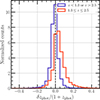 |
Fig. B.1. Difference in photo-z for galaxies from COSMOS2020 re-fitted with LePHARE using just the DAWN PL bands compared to the original COSMOS2020 (Weaver et al. 2022) values. The redshift range 1.3 ≤ z ≤ 2.5 shows greater spread with a tendency towards higher redshifts, especially in the wings, due to lack of constraint on both the Lyman break and Balmer break. Galaxies outside this interval do not have the same problem and constrain at least one of the two breaks. A small number of galaxies scattering to higher redshifts can affect the observed galaxy SMF in this redshift interval. |
Even without a bias towards higher-redshift solutions, the prospect of a low-redshift galaxy (e.g. at z = 1.2) being placed at higher redshifts (e.g. to z = 2) presents an effect that is observed more often than the inverse. At fixed mass, galaxies are less abundant at high z at all masses. Thus, the fractional change in the number density is always greater when a galaxy is moved from a low-redshift bin to a higher-redshift bin. In addition, the change in the luminosity distance implies a greater inferred mass for objects being moved to higher redshifts than they would have if placed to a lower redshift, where galaxies are more numerous. This is essentially the Eddington bias, but considered from the perspective of covariance with the redshift. Finally, a randomly selected low-redshift galaxy is more likely to be brighter in the observed-frame, further exacerbating the impact on the observed number density at higher redshifts. It is important to emphasise that, for consistency with D17 and W23, LePHARE was not run with an apparent magnitude prior (or any prior). It is noted that this trend is visible even in Fig. C1 of EC-Z25 in the comparison between the newly obtained photo-z and those presented by Weaver et al. (2022).
B.2. Random-forest-predicted galaxy properties
With a goal to further validate the physical properties of galaxies measured with LePHARE in this work, an additional set of galaxy properties are obtained following the machine learning methods explored by Chartab et al. (2023). Therein, the authors analysed the information content of multi-wavelength galaxy surveys using a combination of an information theory and machine learning techniques. Specifically, the authors investigated the information content of the COSMOS2020 catalogue that is encoded by the photometry measured in the Hawaii Two-0 / DAWN survey PL (EC-Z25) filter set, namely, CFHT MegaCam u, Subaru HSC griz, and Spitzer/IRAC [3.6 μm] and [4.5 μm]. Among other results, the authors showed that for an optically selected catalogue, a random forest regressor (Breiman 2001) can be trained to predict the flux in NIR bands (e.g. UltraVista YJH), photometric redshifts, and stellar masses, each with impressive accuracy. In their work, they trained a random forest regressor on a training sample selected from the COSMOS2020 catalogue and then predicted galaxy properties from a test sample. Their analysis is extended here, where a random forest regressor is trained on the COSMOS2020 catalogue and galaxy properties are predicted from the DAWN PL catalogue.
The basic approach for training the random forest described by Chartab et al. (2023) is followed here. One modification, however, is the selection of galaxies. Rather than splitting the COSMOS2020 catalogue evenly into a training and a test sample, all galaxies that satisfy the basic requirements of signal-to-noise in the appropriate filters (Sect. 3.1) are used to train the random forest to predict photo-zs using photometry from the modified COSMOS2020 catalogue (i.e. just using the DAWN PL filters). However, under this configuration, it was observed that high-redshift solutions were disfavoured too often when comparing the outputs to the LePHARE measurements for the same galaxies. This bias can be seen at z > 2 in Fig. 11 of Chartab et al. (2023). The bias is likely caused by the conservative nature of a random forest: by number, high-redshift galaxies are comparatively rare, and a random forest is prevented from predicting properties outside its training data by construction. To remedy this bias, an alternative selection was used to select an approximately even number of galaxies as a function of redshift. Specifically, redshift-stratified sampling was performed by binning all galaxies meeting the signal-to-noise requirements in redshift-space with a bin size of δz = 0.1 and setting the maximum number of galaxies in each bin to the number in the 4 < z ≤ 4.1 bin (selected as a reference point). Within each δz bin, galaxies are randomly selected. This approach preferentially retains nearly all available z ≥ 4 galaxies while subsampling the more numerous low-z population. The downside to this approach is that it removes a significant portion of the training sample and creates a challenge for evaluating the performance of the random forest.
The random forest is first trained to predict redshifts from the modified COSMOS2020 catalogue. As described above, evaluating the performance of the random forest predictions is a challenge given the selection of the training set. For the performance of the model under similar conditions and a standard training/testing split, the reader is directed to Chartab et al. (2023). In this case, to provide insight into the performance of the model, the modified COSMOS2020 catalogue is used and the photometry is perturbed. First, the photometric uncertainties are scaled according to the method described by EC-Z25 to match the flux-flux uncertainty relationships of DAWN PL. Then, each flux is scattered assuming a Gaussian probability distribution centred on the flux and with a standard deviation equal to the scaled flux uncertainty. The result of applying the random forest to this perturbed photometry from COSMOS2020 is shown in the top row of Fig. B.2 for galaxies that have sufficient signal-to-noise in the necessary bands (Sect. 3.1) and that are above the nominal stellar mass limit (Sect. 3.3). The x-axis is the official COSMOS2020 redshift (column name: ‘lp_zPDF’) and the y-axis is the random-forest prediction. Colour scaling shows logarithmic density. Generally, the agreement is excellent, although it is emphasised that photo-zs obtained from re-fitting the modified COSMOS2020 catalogue with LePHARE are better for the faintest galaxies, with 5.4% outliers in comparison to 6.1%. One area of improvement obtained by the random forest is in the redshift range 1.5 < z ≤ 2.5, in which there is no significant bias. Although there is scatter, it appears approximately equal in each direction, whereas the values from LePHARE show a small bias towards higher redshifts (Fig. B.1).
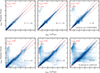 |
Fig. B.2. Top: Validation of photometric redshifts (photo-z) predicted from a random forest regressor trained on photometry from the COSMOS2020 in the DAWN PL filter set. The y-axis shows the random-forest-predicted redshifts after scattering the photometry within the photometric errors, while the x-axis shows the official Weaver et al. (2022) photo-z measured with LePHARE and > 40 photometric bands. Galaxies are selected for this comparison using the criteria described in Sect. 3.1. Bottom: Comparison of photo-zs predicted from DAWN PL photometry using the random forest trained on COSMOS2020 as described above. The y-axis shows the random-forest-predicted redshifts from DAWN PL, while the x-axis shows the redshift measured from LePHARE using the same photometry provided by EC-Z25. Galaxies selected for this validation also satisfy the requirements of Sect. 3.1. Shading corresponds to logarithmic density. |
The random forest trained on the modified COSMOS2020 catalogue is next used to predict galaxy properties from the DAWN PL photometry. Before doing so, photometric offsets are determined and applied to every photometric filter based on the median colours of stars in each field. Stars are identified from both COSMOS2020 and DAWN PL (with EDF-N and EDF-F treated separately) based on the χ2 of the best-fit LePHARE stellar and galaxy templates. Only stars with signal-to-noise greater than 10 are used for this calibration. Then, median differences in each available colour are measured (i.e. with seven available filters, there are six independent colours) between DAWN PL and COSMOS2020. Finally, a system of equations is solved to determine a linear offset for each band that minimises the median difference in each colour measured between COSMOS2020 and DAWN PL. The resulting offsets are less than ∼5% with the exception of Spitzer/IRAC [4.5 μm], which is ∼15%. Overall, these are of similar scale to what is obtained from LePHARE when fixing the redshifts of a spectroscopic sample to their spectroscopic values and minimising the differences in the photometry predicted by the best-fit LePHARE galaxy templates (e.g. Weaver et al. 2022, Table 3; see also Ilbert et al. 2013 and Laigle et al. 2016 for further description of this operation). The random-forest-predicted redshifts for DAWN PL are shown in the bottom row of Fig. B.2 (y-axis) and compared to the photo-z measured with LePHARE for the same galaxies (x-axis). The same selection criteria are applied as for the row above (i.e. those described in Sect. 3.1). It should not be expected that the redshifts from the random forest predictions and LePHARE agree in DAWN PL as well as they do for COSMOS because random forest was trained to predict the exact redshifts used in the comparison. Nonetheless, the random-forest-predicted redshifts for DAWN PL agree well with the values obtained from LePHARE, and for the entire sample generally. Indeed, the agreement is similar to what Weaver et al. (2022) showed when comparing the output from fitting the same exact photometry with the two separate SED-fitting codes, LePHARE and EAZY (see e.g. their Fig. 14). Interestingly, a number of bright galaxies (17 < i < 24) that are moved from higher-redshift solutions to low-redshift solutions by the random forest. As will be shown below, this largely solves the excess of massive galaxies seen in the DAWN PL galaxy SMF at 1.5 < z ≤ 2.5.
Departing from Chartab et al. (2023), stellar masses are determined separately from the photo-z. A second random forest is trained using the modified COSMOS2020 photometry as well as the official Weaver et al. (2022) photo-z values as inputs, and the training target is the stellar mass. The primary reason for separating these steps is to exploit the information in the redshift related to the stellar mass, i.e. the luminosity distance. This also ensures that the predicted stellar mass is consistent with the observed distribution of redshift versus stellar mass provided by the COSMOS2020 catalogue, which is not as likely if the stellar mass is predicted without knowledge of the redshift. For the purposes of validation, stellar masses are predicted from the modified COSMOS2020 catalogue, again with photometry scattered within the photometric uncertainties, and the photo-zs predicted by the random forest in the previous step as inputs. The result is shown in the left-hand side of Fig. B.3 for galaxies that have sufficient signal-to-noise in the necessary bands (Sect. 3.1) and that are above the nominal stellar mass limit (Sect. 3.3). In addition, galaxies are selected to have redshifts that agree within 0.15(1 + δz) to avoid differences that would arise simply from discrepant redshifts. The x-axis is the official COSMOS2020 stellar mass (column name: ‘lp_mass_best’) and the y-axis is the difference in stellar mass from the prediction and the official value. colour scaling shows logarithmic density, and the red shading shows the 1σ spread. The agreement is again strong. In this case, it appears that the random-forest performs equally well compared to SED fitting (e.g. EC-Z25, Fig. 11). However, without utilising the redshift as an input, the quality of the random forest prediction degrades.
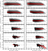 |
Fig. B.3. Left: Validation of stellar masses predicted from a random forest regressor trained on photometry from the COSMOS2020 in the DAWN PL filter set. The y-axis shows the difference in stellar mass between the random-forest-predicted values, after scattering the photometry within the photometric errors, and the official Weaver et al. (2022) stellar masses measured with LePHARE and greater than 40 photometric bands. The x-axis shows the official Weaver et al. (2022) stellar masses. Galaxies are selected for this comparison using the criteria described in Sect. 3.1. Right: Comparison of stellar masses predicted from DAWN PL photometry using the random forest trained on COSMOS2020 as described above. The y-axis shows the difference in stellar mass between the random-forest-predicted values from DAWN PL and the stellar masses measured from LePHARE using the same photometry provided by EC-Z25. The x-axis shows the LePHARE stellar mass. Galaxies selected for this validation also satisfy the requirements of Sect. 3.1. Shading corresponds to logarithmic density. |
The random forest trained on the modified COSMOS2020 catalogue is next used to predict stellar masses from the DAWN PL photometry and from the random-forest-predicted redshifts. The same linear offsets applied to the photometry before predicted the redshifts are used again. The random-forest-predicted stellar masses for DAWN PL are compared to the values measured from LePHARE in the right-hand side of Fig. B.3. The same selection criteria are applied as for the row above, i.e. those described in Sect. 3.1, and the requirement that redshifts that agree within 0.15(1 + δz). At z < 4, the agreement with the values determined with LePHARE is nearly as good as in the COSMOS2020 validation shown in the left-hand side, without any bias. Starting at 4 < z < 5, a bias begins to appear for the most massive galaxies, where the random forest predicts a smaller stellar mass than is determined with LePHARE. As can be seen from the left-hand panel (as well as Fig. 6), there are very few galaxies with stellar masses ℳ ≳ 1011 M⊙ in COSMOS2020 at z > 4. As such, the random forest is biased against predicting such great stellar masses because such galaxies are largely absent from the training data. However, it is expected that over the entire DAWN PL volume, which is an order of magnitude larger than COSMOS2020, there should be many intrinsically bright galaxies at high redshifts. Indeed, at every redshift interval, the most massive galaxies are found to be less massive according to the random forest, even in the training data. Care must therefore be taken when considering galaxy properties inferred from machine learning techniques.
As a whole, the random-forest-predicted quantities appear mostly reasonable, with the exception of the highest-redshift bins. Nonetheless, having calculated these values, it is possible to measure the evolution of the SMF using the same stellar mass bins and redshift bins as above. The result is shown in Fig. B.4 for z ≤ 3.5 and Fig. B.5 for z > 3.5, alongside the values from re-fitting the modified COSMOS2020 catalogue with LePHARE, the observed galaxy SMF from DAWN PL, and the results of D17 and W23.
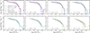 |
Fig. B.4. Same as Fig. 5 but with additional data points from the random forest (squares) and COSMOS2020 re-fits (triangles). Due to the conservative nature of random forests, large stellar masses are generally disfavoured at all redshifts. At 1.1 < z ≤ 2.5, this appears to correct for the bias observed from LePHARE alone, but at z > 2.5, this appears to lead to an incompleteness. COSMOS2020 re-fitted using just the DAWN PL bands closely resembles the DAWN PL observed galaxy SMF. |
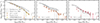 |
Fig. B.5. Same as Fig. 6 but showing additional data points from the random forest (squares) and the COSMOS2020 re-fits (triangles), as in Fig. B.4. |
At z ≤ 3.5, there is strong agreement with DAWN PL, the result of re-fitting the COSMOS2020 catalogue, with D17. The agreement with W23 is similar to what is achieved with DAWN PL. Overall, this exercise is another confirmation that there is sufficient information present in the DAWN PL catalogues to reliably infer the evolution of the galaxy SMF. As noted previously, the random-forest-predicted values also successfully avoid the excess in massive galaxies seen at 1.5 < z ≤ 2.5. Referring back to Fig. B.2, the problematic galaxies are likely placed at lower redshifts. At z > 3.5, the random forest appears poorly suited to measure the galaxy SMF. The stellar mass limit is high for DAWN PL (i.e. ℳ ≳ 1010 M⊙ at z ∼ 4). Such galaxies are relatively rare in the training data (COSMOS2020) by absolute number. As such, lower stellar masses are preferred by the random forest, as are lower-redshift solutions, severely impacting the high-redshift galaxy SMF.
Given the improvement at low redshifts, it may be advantageous to somehow utilise the random-forest-predicted galaxy properties alongside those obtained through SED fitting. However, it is not obvious how best to do so without introducing additional biases and systematic uncertainties to the analysis. A future work may explore this topic more fully.
All Tables
Total co-moving volume, stellar mass limit (for the total sample), and number of galaxies with stellar masses above the stellar mass limit for each redshift bin.
Double (z ≤ 2) and single (z > 2) Schechter parameters derived for the total mass-complete sample.
Double (z ≤ 2) and single (z > 2) Schechter parameters derived for the star-forming mass-complete subsample.
Double (z ≤ 0.8) and single (z > 0.8) Schechter parameters derived for the quiescent mass-complete subsample.
All Figures
|
Fig. 1. Galaxies identified as either star-forming or quiescent based on their NUV − r and r − J rest-frame colours at z ≤ 3. Rest-frame colours are measured using LePHARE following Ilbert et al. (2005). Representative uncertainties associated with the rest-frame colours of the star-forming (blue) and quiescent (maroon) subsamples are plotted. At z > 1.5, the Balmer break is redshifted between two observed bands (HSC z and IRAC [3.6 μm]), and so the inferred rest-frame colours become increasingly model-dependent. Shading corresponds to logarithmic density. |
| In the text | |
|
Fig. 2. Galaxy stellar mass distribution as a function of redshift. The limiting stellar mass of the total (left), star-forming (middle), and quiescent (right) samples are determined as a function of redshift following Pozzetti et al. (2010) and are shown by the solid black curves. Two estimates are computed based on the limiting magnitude of HSC z (solid) and the IRAC [3.6 μm] limiting magnitude (dotted), respectively. The more conservative estimate using HSC z is used in the remainder of this work and are presented as Eqs. (3)–(5) for the total, star-forming, and quiescent samples. For comparison, the stellar mass limits of D17 and W23 are also shown. Shading corresponds to logarithmic density. |
| In the text | |
|
Fig. 3. Three components of the total uncertainty of the number density in each ℳ bin, σΦ: the Poisson uncertainty (σN; left), cosmic variance (σCV; middle), and uncertainty arising from SED fitting (σSED; right). The total uncertainty, shown by the dashed lines in each panel, is the quadrature sum of the three components, shown by the solid lines in each panel. |
| In the text | |
|
Fig. 4. Evolution of the observed galaxy SMF of the total sample across 0.2 < z ≤ 6.5. The ℳ bins are uniform except for the first bin, which is extended to the respective stellar mass limit. The ℳ bins below the stellar mass limit (Eq. 3) are not shown. Uncertainties are indicated by the solid error bars and shaded regions. |
| In the text | |
|
Fig. 5. Observed total galaxy SMF of DAWN PL (coloured points) and uncertainties (1σ, shaded) compared with two measurements from COSMOS, D17 and W23, through to 3 < z ≤ 3.5. ℳ bins below the stellar mass limit (Eq. 3) are not shown. The volume limit according to the N = 0 Poisson uncertainty is shown by the downward pointing coloured arrow for DAWN PL and in grey for W23. |
| In the text | |
|
Fig. 6. Same as Fig. 5 but at z > 3.5 and also showing measurements from G15 with HST (grey circles) and W24 with JWST (grey squares). |
| In the text | |
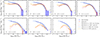 |
Fig. 7. Same as Fig. 5 but comparing the SMFs of star-forming and quiescent galaxies until z ≤ 3. |
| In the text | |
|
Fig. 8. Variation in the best-fit double Schechter function resulting from three different parameterisations of the uncertainty in ℳ used for the Eddington bias kernel (Eq. (11)) at 1.1 < z ≤ 1.5. The shape of the kernel according to each parameterisation is shown in the inset plot, with the corresponding parameter values annotated above in matching colours. The resulting intrinsic (solid) and observed (dotted) galaxy SMF is shown for each case, with the value of the best-fit characteristic mass (ℳ★) annotated and given by the vertical dashed lines. The treatment of the Eddington bias significantly affects the inferred intrinsic galaxy SMF. |
| In the text | |
|
Fig. 9. Evolution of the intrinsic galaxy SMF of the total sample, shown as solid lines, across 0.2 < z ≤ 6.5. Maximum a posteriori values are assumed, as listed in Table A.1. The 1σ (2σ) uncertainty according to the variation in the MCMC chains is shown by the dark (light) shaded regions. Extrapolations below the stellar mass limit (Eq. (3)) are shown by the dashed lines, and the uncertainties are indicated by the hatched regions. Observed values for corresponding redshift bins are shown in the matching colour as data points with error bars. |
| In the text | |
|
Fig. 10. Same as Fig. 9 but separated into star-forming (left) and quiescent galaxies (right) at z ≤ 3. |
| In the text | |
|
Fig. 11. SMD, ρ★, obtained from integrating the intrinsic galaxy SMF (from ℳ = 108 M⊙ to ℳ = 1013 M⊙), shown for both the median posterior values (circle symbols and solid line) and the maximum a posteriori values (square symbols). Values are compared with measurements from the literature also derived from galaxy SMFs (Caputi et al. 2011; González et al. 2011; Santini et al. 2012; Ilbert et al. 2013; Muzzin et al. 2013; Tomczak et al. 2014; Grazian et al. 2015; Caputi et al. 2015; Wright et al. 2018; Bhatawdekar et al. 2019; Adams et al. 2021; McLeod et al. 2021; Thorne et al. 2021; Stefanon et al. 2021; Weaver et al. 2023a; Weibel et al. 2024; Shuntov et al. 2025) as well as integrations of the cosmic SFRD functions (Madau & Dickinson 2014; Behroozi et al. 2019). For the latter, a return fraction of 41% (based on the Chabrier 2003 IMF; see Sect. 6.1 of Ilbert et al. 2013) is assumed. For Madau & Dickinson (2014), a shaded area is shown corresponding to return fractions between 25–30% (where the latter value is similar to the Salpeter 1955 IMF). |
| In the text | |
|
Fig. 12. Intrinsic galaxy SMF of the total sample through to 3.0 < z ≤ 3.5 (solid lines) and observed values (data points) with error bars (in matching colours) compared to the Tinker et al. (2008) dark matter HMF assuming a universal baryon fraction and various integrated star-formation (baryon-to-star conversion) efficiencies, ϵ. ℳ bins below the stellar mass limit are not shown. Maximum a posteriori values for the intrinsic galaxy SMFs are assumed. The uncertainty (1σ dark, 2σ light) according to the variation in the MCMC chains is shown by the shaded regions. The dotted coloured line represents the ‘observed’ model of the galaxy SMF, i.e. including the Eddington bias (Sect. 4.3). The shaded grey region corresponds to the number density of galaxies that would require 100% conversion (or greater) of baryons into star. |
| In the text | |
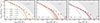 |
Fig. 13. Same as Fig. 12 but at z > 3.5 and also showing additional values of ϵ. |
| In the text | |
|
Fig. 14. Fraction of all galaxies in each ℳ bin in the most dense environments, D4, compared to the least dense environments, D1, relative to unity, ℱ = 1 − N(D1)/N(D4). See the main text for a description of the density estimates. For ℱ < 0, more galaxies are contributed by the least-dense environments; ℱ = 0 implies the two quartiles contribute equally; and ℱ > 0 indicates that more galaxies are contributed by the most dense environments. The solid coloured lines indicates the ratio of the counts in each quartile (subtracted from 1), and the shaded regions correspond to the 1σ uncertainties propagated from σΦ (Sect. 3.4). At low masses (ℳ < 1010 M⊙), more galaxies are found in low-density environments, while galaxies above are preferentially located in high-density environments. The inset plot shows the same relationship for 0.8 < z ≤ 1 separated into star-forming and quiescent galaxies. The over-abundance of low-mass quiescent galaxies in high-density environments is indicative of ‘environment quenching’ (Peng et al. 2010, 2012). |
| In the text | |
|
Fig. 15. Illustrative data for two galaxies observed by DAWN PL. See the main text for details. Top: Most massive galaxy from DAWN PL with a reliable spectroscopic redshift at z > 3, with log10(ℳ/M⊙) = 11.1 ± 0.1. The galaxy is located in EDF-F (which does not include HSC y imaging) and the reported ID corresponds to the DAWN PL EDF-F catalogue. The spectroscopic redshift is obtained from cross-matching to with GOODS-S catalogue (Garilli et al. 2021; Kodra et al. 2023). Bottom: Most massive galaxy observed at 4.5 < z ≤ 5.5. The stellar mass is highly uncertain at |
| In the text | |
|
Fig. B.1. Difference in photo-z for galaxies from COSMOS2020 re-fitted with LePHARE using just the DAWN PL bands compared to the original COSMOS2020 (Weaver et al. 2022) values. The redshift range 1.3 ≤ z ≤ 2.5 shows greater spread with a tendency towards higher redshifts, especially in the wings, due to lack of constraint on both the Lyman break and Balmer break. Galaxies outside this interval do not have the same problem and constrain at least one of the two breaks. A small number of galaxies scattering to higher redshifts can affect the observed galaxy SMF in this redshift interval. |
| In the text | |
|
Fig. B.2. Top: Validation of photometric redshifts (photo-z) predicted from a random forest regressor trained on photometry from the COSMOS2020 in the DAWN PL filter set. The y-axis shows the random-forest-predicted redshifts after scattering the photometry within the photometric errors, while the x-axis shows the official Weaver et al. (2022) photo-z measured with LePHARE and > 40 photometric bands. Galaxies are selected for this comparison using the criteria described in Sect. 3.1. Bottom: Comparison of photo-zs predicted from DAWN PL photometry using the random forest trained on COSMOS2020 as described above. The y-axis shows the random-forest-predicted redshifts from DAWN PL, while the x-axis shows the redshift measured from LePHARE using the same photometry provided by EC-Z25. Galaxies selected for this validation also satisfy the requirements of Sect. 3.1. Shading corresponds to logarithmic density. |
| In the text | |
|
Fig. B.3. Left: Validation of stellar masses predicted from a random forest regressor trained on photometry from the COSMOS2020 in the DAWN PL filter set. The y-axis shows the difference in stellar mass between the random-forest-predicted values, after scattering the photometry within the photometric errors, and the official Weaver et al. (2022) stellar masses measured with LePHARE and greater than 40 photometric bands. The x-axis shows the official Weaver et al. (2022) stellar masses. Galaxies are selected for this comparison using the criteria described in Sect. 3.1. Right: Comparison of stellar masses predicted from DAWN PL photometry using the random forest trained on COSMOS2020 as described above. The y-axis shows the difference in stellar mass between the random-forest-predicted values from DAWN PL and the stellar masses measured from LePHARE using the same photometry provided by EC-Z25. The x-axis shows the LePHARE stellar mass. Galaxies selected for this validation also satisfy the requirements of Sect. 3.1. Shading corresponds to logarithmic density. |
| In the text | |
|
Fig. B.4. Same as Fig. 5 but with additional data points from the random forest (squares) and COSMOS2020 re-fits (triangles). Due to the conservative nature of random forests, large stellar masses are generally disfavoured at all redshifts. At 1.1 < z ≤ 2.5, this appears to correct for the bias observed from LePHARE alone, but at z > 2.5, this appears to lead to an incompleteness. COSMOS2020 re-fitted using just the DAWN PL bands closely resembles the DAWN PL observed galaxy SMF. |
| In the text | |
|
Fig. B.5. Same as Fig. 6 but showing additional data points from the random forest (squares) and the COSMOS2020 re-fits (triangles), as in Fig. B.4. |
| In the text | |
Current usage metrics show cumulative count of Article Views (full-text article views including HTML views, PDF and ePub downloads, according to the available data) and Abstracts Views on Vision4Press platform.
Data correspond to usage on the plateform after 2015. The current usage metrics is available 48-96 hours after online publication and is updated daily on week days.
Initial download of the metrics may take a while.