| Issue |
A&A
Volume 708, April 2026
|
|
|---|---|---|
| Article Number | A90 | |
| Number of page(s) | 19 | |
| Section | Planets, planetary systems, and small bodies | |
| DOI | https://doi.org/10.1051/0004-6361/202555931 | |
| Published online | 30 March 2026 | |
The GAPS Programme at the TNG
LXXII. TOI-5734b: A hot sub-Neptune orbiting a relatively young K dwarf with an Earth-like density★
1
INAF – Osservatorio Astronomico di Roma,
Via Frascati 33,
00040
Monte Porzio Catone (RM),
Italy
2
Dipartimento di Fisica, Università di Roma Tor Vergata,
Via della Ricerca Scientifica 1,
00133
Roma,
Italy
3
Dipartimento di Fisica, Sapienza Università di Roma,
Piazzale Aldo Moro 5,
00185
Roma,
Italy
4
Max Planck Institute for Astronomy,
Königstuhl 17,
69117
Heidelberg,
Germany
5
Department of Astronomy, Sofia University “St Kliment Ohridski”,
5 James Bourchier Blvd,
1164
Sofia,
Bulgaria
6
Landessternwarte, Zentrum für Astronomie der Universtät Heidelberg,
Königstuhl 12,
69117
Heidelberg,
Germany
7
INAF – Osservatorio Astrofisico di Torino,
Via Osservatorio 20,
10025
Pino Torinese,
Italy
8
ESO – European Southern Observatory,
Alonso de Córdova 3107, Casilla 19,
Santiago
19001,
Chile
9
INAF – Osservatorio Astronomico di Palermo,
Piazza del Parlamento 1,
90134
Palermo,
Italy
10
Centre for Astrophysics | Harvard & Smithsonian,
60 Garden Street,
Cambridge,
MA
02138,
USA
11
Fundación Galileo Galilei – INAF,
Rambla José Ana Fernandez Pérez 7,
38712
Breña Baja (TF),
Spain
12
INAF – Osservatorio Astronomico di Padova,
Vicolo dell’Osservatorio 5,
35122
Padova,
Italy
13
INAF – Osservatorio Astrofisico di Catania,
Via S. Sofia 78,
95123
Catania,
Italy
14
Dipartimento di Fisica e Astronomia, Università degli Studi di Padova,
Vicolo dell’Osservatorio 3,
35122
Padova,
Italy
15
Department of Physics and Astronomy, Vanderbilt University,
Nashville,
TN
37235,
USA
16
DISAT, Università degli Studi dell’Insubria,
via Valleggio 11,
22100
Como,
Italy
17
INAF – Osservatorio Astronomico di Brera,
Via E. Bianchi 46,
23807
Merate (LC),
Italy
18
NASA Exoplanet Science Institute-Caltech/IPAC,
Pasadena,
CA
91125,
USA
19
Department of Physics and Kavli Institute for Astrophysics and Space Research, Massachusetts Institute of Technology,
Cambridge,
MA
02139,
USA
20
National Optical-Infrared Astronomy Research Laboratory,
950 N. Cherry Avenue,
Tucson,
AZ
85719,
USA
21
Center for Space and Habitability, University of Bern,
Bern,
Switzerland
22
Sternberg Astronomical Institute, Lomonosov Moscow State University,
119992
Universitetskii prospekt 13,
Moscow,
Russia
23
Planetary Discoveries in Fredericksburg,
VA
22405,
USA
24
NASA Goddard Space Flight Centre,
8800 Greenbelt Rd,
Greenbelt,
MD
20771,
USA
25
Società Astronomica Lunae, Castelnuovo Magra,
Italy
★★ Corresponding author. This email address is being protected from spambots. You need JavaScript enabled to view it.
Received:
13
June
2025
Accepted:
15
February
2026
Abstract
Context. Increasing interest in young exoplanets is leading to a growing effort to understand the formation and evolutionary processes responsible for their different architectures. One interesting target is TOI-5734, a relatively young K3–K4 dwarf star (500−150+300 Myr) showing a transiting candidate in photometric observations followed up with high-resolution spectroscopic data.
Aims. Using both Transiting Exoplanet Survey Satellite (TESS) photometry and High Accuracy Radial velocity Planet Searcher for the Northern hemisphere (HARPS-N) radial-velocity (RV) data, we aim to validate the presence of the companion TOI-5734b, measure its planetary mass, size, and its orbital parameters after having characterised its host star. We then aim to study its possible planetary composition and atmospheric evolution.
Methods. By simultaneously modelling photometry and high-cadence RVs, we measured the radius, mass, and density of TOI-5734b precisely, which were needed in order to reconstruct the evolution of its atmosphere under the high-energy irradiation of its young host. In particular, we employed Gaussian processes (GPs) with a flexible kernel to discriminate between the stellar activity of the young host and planetary signals.
Results. We confirmed the planetary nature of TOI-5734b and measured its orbital period (Pb ~ 6.18 d), radius (Rb = 2.10−0.12+0.12 R⊕), and mass (Mb = 9.1−2.6+2.6 M⊕). By measuring its density (ρb = 0.98−0.30+0.36 ρ⊕) and running atmospheric evolution modelling, we infer that TOI-5734b is close to having a rocky composition and an almost completely depleted primary envelope. We also modelled stellar activity, which points to a rotational period of the star of Prot = 11.09−0.08+0.07 d; this is compatible with its young age. Our results point toward the possibility of considering the target for atmospheric studies with present and future ground- and space-based facilities.
Key words: techniques: photometric / techniques: spectroscopic / planets and satellites: fundamental parameters / planets and satellites: individual: TOI-5734 b / stars: individual: TIC 9989136
Based on observations made with the Italian Telescopio Nazionale Galileo operated on the island of La Palma by the INAF – Fundación Galileo Galilei at the Roque de los Muchachos Observatory of the Instituto de Astrofísica de Canarias (IAC) in the framework of the Large Programme Global Architecture of Planetary Systems (GAPS; PI: Micela, ID: A37TAC_31) and the Large Programme Ariel Mass Survey (ArMS) programme (PI: Benatti, ID: A48TAC_48).
© The Authors 2026
 Open Access article, published by EDP Sciences, under the terms of the Creative Commons Attribution License (https://creativecommons.org/licenses/by/4.0), which permits unrestricted use, distribution, and reproduction in any medium, provided the original work is properly cited.
This article is published in open access under the Subscribe to Open model. This email address is being protected from spambots. You need JavaScript enabled to view it. to support open access publication.
1 Introduction
Thanks to the large number of exoplanets detected so far, we have entered the era of exoplanet demographics and started a systematic investigation of the large variety of physical properties and orbital architectures exhibited by extrasolar planets. In particular, deep interest in their formation processes is rising; this requires solid observational verifications to confirm theoretical models. For this the description of the initial planetesimal and pebble accretion mechanisms is necessary (e.g. Tychoniec et al. 2020), contributing to the formation of terrestrial and giant planets cores and the improvement of core-accretion (Ida & Lin 2004; Matsuo et al. 2007) and disk-instability (Boss 1997; Currie et al. 2022) scenarios, which should be adopted to model the ensuing evolution and accretion of a primary atmosphere. To unravel the mechanisms of planetary formation and evolution and their timescales, the study of infant planets, likely still at their original formation sites, is crucial. This is achieved by analysing and characterising planets in young systems (e.g. Carleo et al. 2020).
Since the Transiting Exoplanet Survey Satellite (TESS; Ricker et al. 2014) began scanning the solar neighbourhood (Benatti et al. 2019; Newton et al. 2019), the number of young planets discovered has increased. This led to the observational focus on high-resolution spectroscopic follow-ups of transiting systems detected by TESS, allowing for the constraint of planetary masses. However, it is still difficult to extract reliable masses for particularly active young stars with strong activity signals in their radial-velocity (RV) time series. Spots, faculae, and other flux variations due to magnetic activity on the stellar surface can completely hide small planetary signals (e.g. Benatti et al. 2021; Carleo et al. 2021; Damasso et al. 2023). Consequently, analytical techniques such as Gaussian processes (GPs; Rasmussen & Williams 2006) must be used to model and remove the stellar influence so that an increasing number of young exoplanets with well-constrained radii and masses can be revealed in combination with a tailored observing strategy (e.g. Nardiello et al. 2022; Barragán et al. 2022; Mallorquín et al. 2023). Furthermore, the choice of the GP kernel is fundamental to face the system-specific data reduction. The most common kernels are the quasi-periodic and double stochastically driven, damped simple harmonic oscillator (dSHO) kernel (Foreman-Mackey et al. 2017; Foreman-Mackey 2018); however, in some cases it could be useful to apply a kernel taking into account the expected wavelength dependence of stellar activity to estimate RV signals below the activity RV noise level (see, e.g. Cale et al. 2021).
The study of small and close-in planets around solar-type stars has led to one of the most relevant observational results: the discovery of a bimodal distribution of planetary radii with a separation region, the ‘radius valley’. It is placed at ~1.7–2.0 M⊕ (e.g. Fulton et al. 2017; Van Eylen et al. 2018) dividing two populations of planets: super-Earths (≲1.8 M⊕) and sub-Neptunes (≳1.8 M⊕). The exact location of the valley may vary depending on the relation of planetary radius with planetary orbital period and stellar mass (Van Eylen et al. 2018; Fulton & Petigura 2018; Petigura et al. 2022). Super-Earths are high-density planets with an expected rocky composition and a null or scarce atmospheric envelope. At the same time, sub-Neptunes are intermediate- and low-density planets whose composition is mostly explained as a core made of icy and rocky material with a shallow H-He atmospheric envelope (‘gas dwarfs’). However, recent findings report greater diversity in the composition of sub-Neptunes, which can be modelled as ‘water worlds’ or ‘steam worlds’, which have a rocky core surrounded by liquid or icy water shells and an envelope of water vapour mixed with H2 and high mean molecular weight volatiles (Luque & Pallé 2022; Piaulet-Ghorayeb et al. 2024; Burn et al. 2024; Bonomo et al. 2025).
The Global Architecture of Planetary System (GAPS) programme at the Telescopio Nazionale Galileo (TNG) was created more than ten years ago (Covino et al. 2013) to provide a comprehensive characterisation of the architectural properties of planetary systems by exploiting RV follow-up observations and a precise and a homogeneous analysis of the stellar atmospheres (e.g. Baratella et al. 2020b; Biazzo et al. 2022; Filomeno et al. 2024) and deriving planetary orbital and physical parameters (e.g. Nardiello et al. 2022; Naponiello et al. 2025; Nardiello et al. 2025). In the framework of GAPS, two observing programmes focused on planets around young stars, relying on high-cadence RV monitoring. The young objects (YOs) sub-programme (Carleo et al. 2020) was aimed at observing young and intermediate-aged stars (from a few megayears to a few gigayears) to detect young exoplanets down to super-Earth masses, including validation and mass measurement of transiting candidates (see, e.g. Nardiello et al. 2025; Mantovan et al. 2024a). After the conclusion of the GAPS-YO sub-programme, the Ariel Masses Survey (ArMS) large programme (PI: Benatti) started its operations, with the aim of measuring the masses of planets with radii spanning the ‘radius valley’ suitable for atmospheric characterisation with the Atmospheric Remote-Sensing Infrared Exoplanet Large-survey (Ariel; Tinetti et al. 2018) Space Mission. In the ArMS sample, several young transiting planets were also included to predict their atmospheric evolution.
In this paper, we present the detection and characterisation of the transiting young planetary system TOI-5734 (TIC 9989136), selected both for the GAPS-YO and the ArMS programmes. The study was performed using a combination of three TESS sectors and spectroscopic data from the High Accuracy Radial velocity Planet Searcher for the Northern hemisphere (HARPS-N, Cosentino et al. 2014) spectrograph installed at the TNG.
The paper is organised as follows: Sect. 2 presents the photometric and spectroscopic observations. Sect. 3 reports the determination of the stellar fundamental parameters. Sect. 4 presents the planet photometric validation. In Sect. 5, we describe the methods for the planetary system analysis and the joint fit results with the retrieved planetary system parameters. We present our discussion in Sect. 6, and in Sect. 7 we summarise our results.
2 Observations and data reduction
2.1 TESS data
The TESS mission observed TOI-5734 (2MASS J07250142 +3713516) with a cadence of 1800 s, 600 s, and 200 s, respectively, for Sectors 20, 47 (starting on February 14, 2020 and February 11, 2022), and 60 (starting on February 7, 2023; programme ID: G05121). The light curves were downloaded from the Mikulski Archive for Space Telescopes1 (MAST), extracted and corrected adopting the PATHOS pipeline (see Nardiello et al. 2019, 2020, 2021; Nardiello 2020). We analysed the light curve extracted with a three-pixel aperture photometry, which is optimal for our target with a TESS magnitude of T ~ 8.5 mag (see Table 1). Moreover, we excluded all the data points in the light curves with the data quality parameter DQUALITY>0 (see the TESS Science Data Products Description Document for details). Further, we cleaned the light curves, removing the remaining outliers distant by more than 4σ from the mean flux and the data points showing a bimodal trend at the beginning of the light curves.
We verified the absence of nearby sources from Data Release 3 (DR3) of the Gaia catalogue (Gaia Collaboration 2016, 2023), possibly contaminating the flux from TOI-5734 in the target pixel files using the code tpfplotter (Aller et al. 2020). We set a specific maximum magnitude contrast of Δm = 8 for our targets and plotted the proper motion directions of all targets. As shown in Fig. 1 for Sector 20, the code highlights the aperture mask that the Science Processing Operations Centre (SPOC) pipeline (Jenkins et al. 2016) employs to measure the simple aperture photometry (SAP) flux. For TOI-5734, many targets are shown in the 10 × 10 px field. The stars with the smallest contrast with TOI-5734 are identified as Gaia DR3 898844472171624576 (G = 14.6 mag) and Gaia DR3 898844575250838400 (G = 13.2 mag), respectively numbered 2 and 3 in Fig. 1. We investigated the possibility that some targets could influence the signal from TOI-5734 by estimating the dilution factor. Since we used a three-pixel photometric aperture for our study, we chose to consider all the targets (7) within three pixels of the target star (i.e. inside the dashed green circle in Fig. 1) for each sector, assuming that the faintest targets do not adequately influence the dilution. As reported in Eq. (6) of Espinoza et al. (2019), the dilution factor is D = 1/(1 + ∑n Fn/FT), where n is the number of contaminating sources, ∑n Fn represents the flux of the contaminating sources in the photometric aperture, and FT is the out-of-transit flux of the target star in a given passband. As flux values, we used the Gaia DR3 integrated RP mean flux in e−/s. For each sector, the dilution factor resulted in D = 0.969, and this value was applied to all light curves. The final light curves used in our analysis are shown in Fig. 2.
Stellar properties of TOI-5734 (TIC 9989136).
2.2 HARPS-N data
The target was observed with HARPS-N at TNG 97 times between 7 October, 2022 and 17 May, 2024, with a median exposure time (texp) of 900 s; so, an average [min, max] signal-to-noise ratio (S/N) at 550 nm of 68 [21, 103] was achieved. We reduced the data with the new offline version of HARPS-N data-reduction software (DRS v3.2.0; Cosentino, priv. comm.). The spectroscopic data of TOI-5734 were extracted using a K2 mask template and a cross-correlation-function (CCF) width of 30 km/s. We obtained RV data with an average uncertainty of 1.6 m/s and a dispersion of around 13.3 m/s. To improve the quality of the analysis, we preferred not to consider the data points with an S/N lower than one-third the maximum S/N in the sample. Furthermore, the DRS provided the values of the bisector inverse slope (BIS) velocity span, line contrast, and line full width at half maximum (FWHM), which we used as indicators of stellar activity. The chromospheric activity index, ![Mathematical equation: $\[\log~ R_{\mathrm{HK}}^{\prime}\]$](/articles/aa/full_html/2026/04/aa55931-25/aa55931-25-eq11.png) , was derived after extracting the S-index2, which was calibrated on the Mount Wilson scale (Baliunas et al. 1995) with the use of the procedure described in Lovis et al. (2011).
, was derived after extracting the S-index2, which was calibrated on the Mount Wilson scale (Baliunas et al. 1995) with the use of the procedure described in Lovis et al. (2011).
In addition, we exploited the software SpEctrum Radial Velocity AnaLyser (SERVAL; Zechmeister et al. 2018) to compare the extracted RVs and errors with the DRS ones. The SERVAL RVs have an average uncertainty of 1.3 m/s and a dispersion of around 14.5 m/s, which are compatible within 1 σ with the DRS data; therefore, we decided to use the latter values. The RVs are shown in Fig. A.2 and presented in Table A.1 together with the BIS span and the ![Mathematical equation: $\[\log~ R_{\mathrm{HK}}^{\prime}\]$](/articles/aa/full_html/2026/04/aa55931-25/aa55931-25-eq12.png) . Since the target was observed twice for some nights, we adopted the RV data with a 0.5-day binning width in the analysis, which is a value sufficiently smaller than the orbital period of the planet (see Sect.4).
. Since the target was observed twice for some nights, we adopted the RV data with a 0.5-day binning width in the analysis, which is a value sufficiently smaller than the orbital period of the planet (see Sect.4).
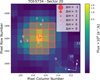 |
Fig. 1 TESS target pixel file of Sector 20 of TOI-5734, which is marked with ‘1’. The other sources, extracted from the Gaia DR3 catalogue, have numbered circles of sizes proportional to the G-mag difference with our target. The colour bar shows the electron counts for each pixel. The orange squares represent the pixels used to construct the aperture photometry by the TESS pipeline. Grey arrows indicate the direction of the proper motions for all the plotted sources. The dashed green circle represents the reference three-pixel aperture to select the targets relevant for the dilution factor estimate. |
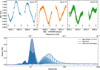 |
Fig. 2 PATHOS light curves of TOI-5734 obtained using TESS data in Sectors 20, 40, and 60, with arrows pointing to the mid-transit times of the planet. The plot below shows the overall GLS and its envelope. The dashed red line represents the signal due to the stellar rotation period peaking at 11.12 d. |
3 Stellar fundamental parameters
3.1 Atmospheric parameters and iron abundance
For the determination of the stellar atmospheric parameters (effective temperature Teff, surface gravity log g, microturbulence velocity ξ) and iron abundance [Fe/H] of TOI-5734, we considered the co-added spectrum obtained through a combination of all spectra collected for the target. The final S/N of the co-added spectrum was ~390 at ~6000 Å.
Given the relatively high level of chromospheric activity of our target, following the same procedure as in Baratella et al. (2020a) and Filomeno et al. (2024) we used a combination of iron (Fe) and titanium (Ti) lines to derive the stellar parameters with the equivalent-width (EW) method. We chose to use Ti lines because of the influence stellar activity might have on Fe lines; i.e. increasing their EWs if they form in the upper layers of the photosphere. This could cause an overestimation of the microturbulence velocity (ξ) and, consequently, an underestimation of the elemental abundances. Instead, Ti lines, which on average form deeper in the photosphere, led to more precise values of ξ (see also Baratella et al. 2020b).
We measured the EWs of both Fe and Ti lines in the neutral and ionised stages using the ARES code (Sousa et al. 2015) and discarded those lines with uncertainties larger than 10%. For lines with EW > 120 mÅ, we double checked the measurements with IRAF3 by fitting Voigt profiles, which better reproduce the line profiles. The line list comes from Baratella et al. (2020a). We adopted the 1D LTE Kurucz model atmospheres linearly interpolated from the Castelli & Kurucz (2003) grid with solar-scaled chemical composition and new opacities (ODFNEW). To derive final stellar parameters and iron abundances, we used the pyMOOGi code by Adamow (2017), which is a Python wrapper of the MOOG code (Sneden 1973, version 2019). The final results of this spectroscopic analysis are reported in Table 1.
Our final spectroscopic temperature agrees, within the uncertainties, with that obtained from photometry, with 2MASS (Cutri et al. 2003) and Gaia DR3 (Gaia Collaboration 2023) magnitudes, and considering the reddening derived through the extinction maps by Lallement et al. (2018) is negligible (E(B − V)=![Mathematical equation: $\[0.000_{-0.000}^{+0.014}\]$](/articles/aa/full_html/2026/04/aa55931-25/aa55931-25-eq13.png) ). Indeed, by using the COLTE program developed by Casagrande et al. (2021), the photometric temperature ranges between 4604 ± 80 K in (GRP − J) and 4706 ± 44 K in (GBP − H) and has a weighted mean value of Teff (phot) = 4670 ± 43 K, as also reported in Table 1. From the mass value reported in the TICv8.2 Catalogue (Paegert et al. 2022) and the photometric Teff, we obtained a log g of 4.64 ± 0.10 dex using the classical equation based on the luminosity of the star, in agreement with our spectroscopic value. With these values and from the relation published by Dutra-Ferreira et al. (2016), the expected ξ is 0.66 ± 0.10 km/s, again in agreement with the spectroscopic estimation (see Table 1). The derived stellar Teff is compatible with a K3–K4 dwarf star (see Pecaut & Mamajek 2013, v.2022).
). Indeed, by using the COLTE program developed by Casagrande et al. (2021), the photometric temperature ranges between 4604 ± 80 K in (GRP − J) and 4706 ± 44 K in (GBP − H) and has a weighted mean value of Teff (phot) = 4670 ± 43 K, as also reported in Table 1. From the mass value reported in the TICv8.2 Catalogue (Paegert et al. 2022) and the photometric Teff, we obtained a log g of 4.64 ± 0.10 dex using the classical equation based on the luminosity of the star, in agreement with our spectroscopic value. With these values and from the relation published by Dutra-Ferreira et al. (2016), the expected ξ is 0.66 ± 0.10 km/s, again in agreement with the spectroscopic estimation (see Table 1). The derived stellar Teff is compatible with a K3–K4 dwarf star (see Pecaut & Mamajek 2013, v.2022).
3.2 Lithium abundance
We measured the EW of the lithium line at 6707.8 Å with IRAF from the co-added spectrum, which resulted in EWLi = 3.3 ± 0.3 mÅ. From this EW and the adopted atmospheric parameters, we estimated the lithium abundance by applying the corrections for non-local thermodynamic equilibrium (NLTE) effects by following the prescriptions of Lind et al. (2009). We obtained an upper limit of 0.04 dex. Despite the almost depleted lithium value, this upper limit seems to support an age following the distribution of young clusters such as Hyades (~600 Myr). Our age estimate is discussed in Sect. 3.6.
3.3 Rotation period
We estimated the stellar rotation period, Prot, both from photometric and spectroscopic data, making use of the generalised Lomb–Scargle (GLS; Zechmeister & Kürster 2009) periodogram4. The results are shown in the bottom panel of Fig. 2 and in Fig. 3 for the joint TESS light curve and spectroscopic data, respectively. The former shows a peak at around 11.12 d, while the latter shows the RV and BIS span periodograms both having a mean peak at Prot = 11.09 ± 0.02 d (respectively, FAP~10−10 and FAP~10−8), which is close to the values extracted from the photometric data. This result is consistent with the significant correlation measured between the RVs and BIS span (Spearman correlation coefficient ρspear = −0.69), suggesting the influence of the stellar activity on the RVs (see also Sect. 5).
3.4 Chromospheric and coronal activity
We measured the activity indices linked to Ca II H & K emission lines, which are the S-index and the ![Mathematical equation: $\[\log~ R_{\mathrm{HK}}^{\prime}\]$](/articles/aa/full_html/2026/04/aa55931-25/aa55931-25-eq14.png) , and they show mean values of 0.72 ± 0.12 dex and −4.47 ± 0.09 dex, respectively. Despite the weak correlation between RVs and the
, and they show mean values of 0.72 ± 0.12 dex and −4.47 ± 0.09 dex, respectively. Despite the weak correlation between RVs and the ![Mathematical equation: $\[\log~ R_{\mathrm{HK}}^{\prime}\]$](/articles/aa/full_html/2026/04/aa55931-25/aa55931-25-eq15.png) (Spearman correlation coefficient ρspear = 0.27), the GLS of
(Spearman correlation coefficient ρspear = 0.27), the GLS of ![Mathematical equation: $\[\log~ R_{\mathrm{HK}}^{\prime}\]$](/articles/aa/full_html/2026/04/aa55931-25/aa55931-25-eq16.png) in Fig. 3 shows strong power at long periods, and an increasing trend in the
in Fig. 3 shows strong power at long periods, and an increasing trend in the ![Mathematical equation: $\[\log~ R_{\mathrm{HK}}^{\prime}\]$](/articles/aa/full_html/2026/04/aa55931-25/aa55931-25-eq17.png) is evident from its time series reported in the bottom panel of Fig. A.2. Here, a possible turnover is observed, and the minimum and maximum values of the time series are
is evident from its time series reported in the bottom panel of Fig. A.2. Here, a possible turnover is observed, and the minimum and maximum values of the time series are ![Mathematical equation: $\[\log~ R_{\mathrm{HK}}^{\prime}\]$](/articles/aa/full_html/2026/04/aa55931-25/aa55931-25-eq18.png) = −4.52 and −4.43, respectively. These considerations were taken into account when calculating the uncertainties of these Ca II activity indices. The star could have a long-term activity cycle, whose periodicity cannot be well defined because of the short time coverage of our dataset. After removing the long-term trend, a significant periodicity at 11.17 d, ascribable to the rotation period of the star, appears on the residuals of the
= −4.52 and −4.43, respectively. These considerations were taken into account when calculating the uncertainties of these Ca II activity indices. The star could have a long-term activity cycle, whose periodicity cannot be well defined because of the short time coverage of our dataset. After removing the long-term trend, a significant periodicity at 11.17 d, ascribable to the rotation period of the star, appears on the residuals of the ![Mathematical equation: $\[\log~ R_{\mathrm{HK}}^{\prime}\]$](/articles/aa/full_html/2026/04/aa55931-25/aa55931-25-eq19.png) time series.
time series.
The Chandra source catalogue v2.0 (source ID 2CXO J072501.4+371352; Evans et al. 2010) includes TOI-5734, which is revealed at 5.4 σ in a shallow observation. More recently, it was also detected in the eROSITA All-Sky Survey (source ID 1eRASS J072501.0+371400; Merloni et al. 2024), with a count rate of 0.143 ± 0.045 cts/s. Adopting an isothermal model for an optically thin plasma, the flux in the standard ROSAT band ([0.1,2.4]keV) can be estimated in the [0.9, 2.5]×10−13 erg/s/cm2 range, depending on the assumed plasma temperature ([2, 10] MK) and metallicity ([0.2, 1] in solar units). These values correspond to an X-ray luminosity of LX = [2, 3] × 1028 erg/s at the distance of the star, and to log LX/Lbol in the [−4.53, −4.36] range from the stellar luminosity derived in Sect. 3.7. In the following, we assume LX = (2.0 ± 0.5) × 1028 erg/s. This value provides the best agreement with the independent predictions based on the measured rotational period (Pizzolato et al. 2003) and on the Ca II ![Mathematical equation: $\[R_{\mathrm{HK}}^{\prime}\]$](/articles/aa/full_html/2026/04/aa55931-25/aa55931-25-eq20.png) (Mamajek & Hillenbrand 2008) within a factor of 1.4.
(Mamajek & Hillenbrand 2008) within a factor of 1.4.
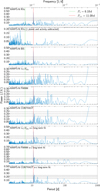 |
Fig. 3 GLS power spectrum for TOI-5734 based on HARPS-N RVs, stellar activity indicators (BIS span, |
![Mathematical equation: $\[\log~ R_{\mathrm{HK}}^{\prime}\]$](/articles/aa/full_html/2026/04/aa55931-25/aa55931-25-eq21.png)
3.5 Kinematic and multiplicity
From the results obtained in the previous sections, TOI-5734 emerges as a relatively young star. We checked membership to nearby young moving groups exploiting the online tool BANYAN Σ5 (Gagné et al. 2018). The star results in a field object with a null membership probability to known groups. The kinematic parameters U, V, and W were derived following the prescriptions of Johnson & Soderblom (1987) and are listed in Table 1. TOI-5734 is close to the edge of the kinematic space typical of young stars (Montes et al. 2001), with properties similar to the Ursa Major moving group. This is fully consistent with the age determinations of other methods.
We also searched for co-moving objects in Gaia DR3. None were found within 600 arcsec (about 20000 au), which is a plausible maximum limit for bound companions. Also, the standard diagnostic used to signify departure from a good single-star model in the Gaia DR3 astrometric solution, the renormalised unit weight error (RUWE), is reported to be 0.930 for TOI-5734 (RUWE>1.4 being the threshold for likely presence of orbital motion in the data), and the RV difference between Gaia DR3 and HARPS-N is not significant. Hence, TOI-5734 appears to be a single star.
3.6 Age
As expected for an unevolved K dwarf, isochrone fitting provides little constraint on stellar age (3.7 ± 3.5 Gyr) using the PARAM6 (da Silva et al. 2006) web interface with the parameters described in Sect. 3.7 and without priors on stellar age. However, as mentioned in previous sections, all indirect age indicators agree quite well and support an age close to and likely slightly younger than that of the Hyades.
The gyrochronology calibration from Mamajek & Hillenbrand (2008) yields an age of 524 ± 25 Myr. Using the Mamajek & Hillenbrand (2008) activity-age relation and the activity values measured in Sect. 3.4, we derived a chromospheric age of 493 ± 300 Myr. The X-ray emission of the star is slightly above the median value of Hyades members of similar colour but within the distribution of available measurements for cluster members, with the nominal age from Mamajek & Hillenbrand (2008) of ![Mathematical equation: $\[360_{-70}^{+110}\]$](/articles/aa/full_html/2026/04/aa55931-25/aa55931-25-eq22.png) Myr.
Myr.
Another age estimate was performed following the methodology described in Jeffries et al. (2023) and using the Empirical AGes from lithium Equivalent widthS (EAGLES) code. In particular, the latter uses the lithium EW at λ6707 Å and the stellar effective temperature. For TOI-5734, we measured the lithium EW of 3.3 ± 0.3 mÅ. Considering that the EAGLES code is likely to derive lower limits in ages for EWLi lower than 50 mÅ, we estimated a lower age limit of ~310 Myr, which is in agreement with our other estimates. Finally, while inconclusive in providing a well-defined age value, the kinematic parameters are in agreement with the age estimates above. Considering the possible long-term variability of the chromospheric and coronal activity, and systematic uncertainties in the rotational evolution (e.g. Curtis et al. 2020), we adopted ![Mathematical equation: $\[500_{-150}^{+300}\]$](/articles/aa/full_html/2026/04/aa55931-25/aa55931-25-eq23.png) Myr as a conservative estimate of the stellar age.
Myr as a conservative estimate of the stellar age.
3.7 Mass and radius
The stellar mass and radius were determined as in previous papers of the GAPS-YO series (Carleo et al. 2021; Nardiello et al. 2025). For the stellar mass, we exploited the PARAM web interface, adopting the mean between spectroscopic and photometric effective temperature, the [Fe/H] from our spectroscopic analysis, and the V magnitude and parallax π from Table 1, and constraining the age to the range allowed by the indirect methods (300–800 Myr, see Desidera et al. 2015). In this way, we found M⋆ = 0.724 ± 0.009 M⊙, where the quoted error is the one obtained by the PARAM procedure, and it does not include possible systematics uncertainties in the input stellar models.
The stellar radius was derived from the Stefan-Boltzmann law using the above parameters and bolometric corrections by Pecaut & Mamajek (2013). It is R⋆ = 0.639 ± 0.034 R⊙. This determination is basically identical to the value obtained through PARAM (R⋆ = 0.637 ± 0.012 R⊙). Both stellar mass and radius are compatible with an independent determination performed using the broadband spectral energy distribution (SED) of the star and Gaia DR3 parallax (see Appendix B). The corresponding stellar luminosity is L⋆ = 0.181 ± 0.009 L⊙.
3.8 Projected rotational velocity and stellar inclination
We used the spectral-synthesis method to estimate the stellar projected rotational velocity (see Biazzo et al. 2022 for details). With the pyMOOGi code by Adamow (2017) and the stellar parameters Teff, log g, ξ, and [Fe/H] derived in Sect. 3.1, we measured v sin i⋆ = 2.9 ± 0.7 km/s, taking into account the spectral regions around 5400, 6200, and 6700 Å. We also computed the projected rotational velocity by applying the empirical relations found in Rainer et al. (2023) using the FWHM of the CCFs of the analysed spectra as input. Considering Equation (7) for the K5 mask, we obtained v sin i⋆ = 3.2 ± 0.5 km/s, which is comparable with the value from the spectral synthesis. Using the previous estimates of Prot and R⋆, we determined the stellar equatorial velocity veq = 2πR⋆/Prot = 2.9 ± 0.2 km/s. This value is compatible with our measurements of v sin i⋆; thus, the stellar inclination is consistent with ≃90 deg.
4 Transit validation
The TESS mission released an alert about a planetary candidate around TOI-5734 with an orbital period around Prot ~ 6.18 d measured by the SPOC pipeline (Jenkins et al. 2016) and archived on the MAST on August 18, 2022. We studied the transit event by first modelling and removing the stellar variability trend from the reduced light curves. We applied the WOTAN detrending algorithm (Hippke et al. 2019) using, on each light curve, an rspline interpolation with a window-length interval of 12 hours. We investigated the presence of transiting candidates using the TRANSIT LEAST SQUARES package (TLS; Hippke & Heller 2019) to extract the periodogram of the joint detrended light curves, looking for transit periods from 1 to 100 d. In Fig. 4 we show the TLS power spectrum with the main peak indicating an orbital period of Pb = 6.18414 ± 0.00072 d with a signal-detection efficiency (SDE) of ~79, which strongly confirms the presence of a transiting candidate. The other relevant peaks represent only low-order harmonics of the main periodicity. Then, we followed the procedure described by Nardiello et al. (2020) for the in- and out-of-transit centroid analysis to check whether the transit is on our target or associated with a neighbour source. We calculated the differences between the mean centroids by averaging the in- and out-of-transit centroids of each sector. We found that the centroid and the target (at (0,0) coordinates) have compatible positions, within the errors (see Fig. A.1), confirming that the transit signal originates from TOI-5734 itself.
To further validate the planet, we used TRICERATOPS (Giacalone et al. 2021), a Bayesian tool designed for TESS candidates. It evaluates the probability of the nature of the transit signal being planetary by combining information on the transit signal, the target star, and nearby stars from Gaia DR2, considering possible false-positive scenarios. The analysis also checks for instrumental artefacts and background contamination. TRICERATOPS can be applied to TESS data alone or combined with high-resolution contrast imaging for improved constraints. According to Giacalone et al. (2021), a planet candidate is validated if it meets the false-positive probability (FPP) criterion of <0.015 and the nearby false-positive probability (NFPP) of < 10−3. The FPP is defined as 1 − (PTP + PPTP + PDTP + Poth), where PTP stands for transiting planet probability, PPTP for primary TP probability, and PDTP for diluted TP probability, while ![Mathematical equation: $\[\mathrm{NFPP}=P_{\mathrm{NTP}}+P_{\mathrm{NEB}}+P_{\mathrm{NEB x} 2 \mathrm{P}}+P_{\text {oth}}^{\prime}\]$](/articles/aa/full_html/2026/04/aa55931-25/aa55931-25-eq24.png) refers to a nearby star with probabilities associated with a nearby transiting planet (NTP), nearby eclipsing binary (NEB), and an eclipsing binary with double orbital period. Even though the Poth and
refers to a nearby star with probabilities associated with a nearby transiting planet (NTP), nearby eclipsing binary (NEB), and an eclipsing binary with double orbital period. Even though the Poth and ![Mathematical equation: $\[P_{\text {oth}}^{\prime}\]$](/articles/aa/full_html/2026/04/aa55931-25/aa55931-25-eq25.png) probabilities contribute to adding FPP and NFPP together to make one, they are sums of negligible terms, so they were not included in the following considerations. In our analysis of TOI-5734b, we used TESS SPOC PDCSAP light curves from all available sectors, adopting extraction apertures from the light-curve headers. We ran TRICERATOPS 100 times, incorporating contrast curves from NESSI on the 3.5-m WIYN telescope (Kitt Peak National Observatory, USA) to refine our results. Since FPP varies across runs, we computed its median and 84th percentile to confirm that the initial validation was not an outlier. The final results yielded FPP = 2 × 10⁻⁵ and NFPP < 1 × 10⁻⁶, suggesting the planet could be validated. However, the uncertainties (0.7 and 0.01, respectively) warrant caution. The ambiguity in the results likely arises from the presence of a nearby star capable of reproducing the observed transit signal (see Fig. 1 the dilution factor estimated in Sect. 2.1) and is further supported by the validation test probabilities: 52% for a transiting planet (TP), 16% for a primary TP, and 15% for a diluted TP, which accounts for the possibility of a bound companion or background stars. Moreover, untraceable stellar activity effects may impact the accuracy of the transit fit and, consequently, the final results. However, we highlight that it is not possible that the transit signal is due to a bound companion, since this option was excluded from both the kinematic analysis of group membership and the Gaia DR3 analysis, with the target being a field object with astrometric values consistent with a single star (see Sect. 3.5). Also, we excluded the presence of any type of blended eclipsing binary from the analysis of ground-based multi-colour photometry from LCOGT (see Appendix C). In addition, we discarded the possibility for diluted TP, since the in- and out-of-transit analysis and LCOGT photometric observations confirm that the transit signal originates on-target and the fit made on the transit detected by LCOGT reveals a transit depth 1σ consistent with that derived in the analysis described in Sect. 5 (see Appendix C and Fig. C.1). Finally, by analysing the high-resolution imaging results from the near-infrared Palomar-PHARO, and the optical WIYN-NESSI and SAI-Speckle Polarimeter instruments, we excluded the presence of any contaminant, such as Gaia unresolved companions, down to Δmag ~ 5 within 0.2–1.0 arcsec (see Appendix D). Consequently, combining our validation analysis with the information from ground-based seeing-limited photometry, Gaia DR3 data and high-resolution imaging data, we have the evidence to consider the planet validated.
probabilities contribute to adding FPP and NFPP together to make one, they are sums of negligible terms, so they were not included in the following considerations. In our analysis of TOI-5734b, we used TESS SPOC PDCSAP light curves from all available sectors, adopting extraction apertures from the light-curve headers. We ran TRICERATOPS 100 times, incorporating contrast curves from NESSI on the 3.5-m WIYN telescope (Kitt Peak National Observatory, USA) to refine our results. Since FPP varies across runs, we computed its median and 84th percentile to confirm that the initial validation was not an outlier. The final results yielded FPP = 2 × 10⁻⁵ and NFPP < 1 × 10⁻⁶, suggesting the planet could be validated. However, the uncertainties (0.7 and 0.01, respectively) warrant caution. The ambiguity in the results likely arises from the presence of a nearby star capable of reproducing the observed transit signal (see Fig. 1 the dilution factor estimated in Sect. 2.1) and is further supported by the validation test probabilities: 52% for a transiting planet (TP), 16% for a primary TP, and 15% for a diluted TP, which accounts for the possibility of a bound companion or background stars. Moreover, untraceable stellar activity effects may impact the accuracy of the transit fit and, consequently, the final results. However, we highlight that it is not possible that the transit signal is due to a bound companion, since this option was excluded from both the kinematic analysis of group membership and the Gaia DR3 analysis, with the target being a field object with astrometric values consistent with a single star (see Sect. 3.5). Also, we excluded the presence of any type of blended eclipsing binary from the analysis of ground-based multi-colour photometry from LCOGT (see Appendix C). In addition, we discarded the possibility for diluted TP, since the in- and out-of-transit analysis and LCOGT photometric observations confirm that the transit signal originates on-target and the fit made on the transit detected by LCOGT reveals a transit depth 1σ consistent with that derived in the analysis described in Sect. 5 (see Appendix C and Fig. C.1). Finally, by analysing the high-resolution imaging results from the near-infrared Palomar-PHARO, and the optical WIYN-NESSI and SAI-Speckle Polarimeter instruments, we excluded the presence of any contaminant, such as Gaia unresolved companions, down to Δmag ~ 5 within 0.2–1.0 arcsec (see Appendix D). Consequently, combining our validation analysis with the information from ground-based seeing-limited photometry, Gaia DR3 data and high-resolution imaging data, we have the evidence to consider the planet validated.
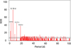 |
Fig. 4 TLS power spectrum of light-curve data of TOI-5734. The transiting signal is confirmed by the peak at Pb=6.18414 d with an SDE value of 79, which is strongly above the thresholds (horizontal dashed lines) corresponding to the TLS false positive rates of 10%, 1%, and 0.1%. |
5 Radial velocity and photometry joint analysis
TOI-5734 is a young, strongly active star, so the RV measurements are likely affected, hiding planetary signals or injecting spurious ones. Hence, it is fundamental to remove the activity contribution from the RVs. To identify if and how stellar-activity signal influences our RV data, we used the BIS span and the ![Mathematical equation: $\[\log~ R_{\mathrm{HK}}^{\prime}\]$](/articles/aa/full_html/2026/04/aa55931-25/aa55931-25-eq26.png) as proxies of the stellar activity. We compared the GLS of the activity indices with that of our data, as shown in Fig. 3. The BIS span has a periodogram peaking at 11.09 d suggesting that its signal is related to the stellar rotation period (see Sect. 3.3) and implies the presence of spots on the stellar surface. Instead, the long-term signal introduced by the
as proxies of the stellar activity. We compared the GLS of the activity indices with that of our data, as shown in Fig. 3. The BIS span has a periodogram peaking at 11.09 d suggesting that its signal is related to the stellar rotation period (see Sect. 3.3) and implies the presence of spots on the stellar surface. Instead, the long-term signal introduced by the ![Mathematical equation: $\[\log~ R_{\mathrm{HK}}^{\prime}\]$](/articles/aa/full_html/2026/04/aa55931-25/aa55931-25-eq27.png) in the RV data (see Sect. 3.4) should not affect the result of our analysis, so we did not use it to model the RVs for the following analysis. As displayed in Fig. 3 for the GLS of FWHM and for contrast, the long-term trend contribution is visible, together with a significant peak at ~30.55 d, showing its alias due to the Moon cycle (clearly visible in the window function). In fact, by removing the long-term trend, the 30.55 d peak goes below the significance thresholds in the GLS of all the activity indicators, as well as the long-term power, and the significance of the rotational period peak strongly increases, as shown in the bottom three panels of Fig. 3. We analysed the system to retrieve the planetary parameters using the toolbox EXO-STRIKER7 (Trifonov 2019). We performed a joint fit of the RV data and the undetrended transit photometry, which were extracted and cleaned through the PATHOS pipeline, and corrected for the dilution factor to consider the flux contamination of the neighbour stars falling inside the photometric aperture (see Sect. 2.1). The transit modelling inside the EXO-STRIKER toolbox was done through the BATMAN package (Kreidberg 2015). We used an algorithm based on GPs to model and remove the signal induced by stellar activity, such as the rotation period signature and the RV long-term trend. Fundamental in this operation was the use of unflattened light curves to exploit the modulation introduced by the stellar rotation. We added the GP regression through the CELERITE package (Foreman-Mackey et al. 2017; Foreman-Mackey 2018) to simultaneously model the stellar activity in both RV and transit signals. After we approached the analysis with a quasi-periodic kernel, we noticed it could not model the relevant harmonic in the GLS of the residuals at half of the stellar rotation period, which is probably a signature of the flux effect on RV variations due to dark spots or bright faculae (see, e.g. Lanza et al. 2010). Therefore, we chose a kernel containing the half-period term in its expression; i.e. the dSHO as defined by Foreman-Mackey et al. (2017) and Foreman-Mackey (2018), because it has two SHO terms that can be used to model stellar rotation and the harmonic at half its period. The kernel hyperparameters are the standard deviation of the process GPdSHO σ, the primary period of variability GPdSHO Prot, the quality factor GPdSHO Q0 (or the quality factor minus one half; this keeps the system underdamped) for the secondary oscillation, and the difference between the quality factors of the first and the second modes GPdSHO dQ. This parametrisation (if dQ > 0) ensures that the primary mode is always of higher quality. In the end, GPdSHO f represents the fractional amplitude of the secondary mode compared to the primary.
in the RV data (see Sect. 3.4) should not affect the result of our analysis, so we did not use it to model the RVs for the following analysis. As displayed in Fig. 3 for the GLS of FWHM and for contrast, the long-term trend contribution is visible, together with a significant peak at ~30.55 d, showing its alias due to the Moon cycle (clearly visible in the window function). In fact, by removing the long-term trend, the 30.55 d peak goes below the significance thresholds in the GLS of all the activity indicators, as well as the long-term power, and the significance of the rotational period peak strongly increases, as shown in the bottom three panels of Fig. 3. We analysed the system to retrieve the planetary parameters using the toolbox EXO-STRIKER7 (Trifonov 2019). We performed a joint fit of the RV data and the undetrended transit photometry, which were extracted and cleaned through the PATHOS pipeline, and corrected for the dilution factor to consider the flux contamination of the neighbour stars falling inside the photometric aperture (see Sect. 2.1). The transit modelling inside the EXO-STRIKER toolbox was done through the BATMAN package (Kreidberg 2015). We used an algorithm based on GPs to model and remove the signal induced by stellar activity, such as the rotation period signature and the RV long-term trend. Fundamental in this operation was the use of unflattened light curves to exploit the modulation introduced by the stellar rotation. We added the GP regression through the CELERITE package (Foreman-Mackey et al. 2017; Foreman-Mackey 2018) to simultaneously model the stellar activity in both RV and transit signals. After we approached the analysis with a quasi-periodic kernel, we noticed it could not model the relevant harmonic in the GLS of the residuals at half of the stellar rotation period, which is probably a signature of the flux effect on RV variations due to dark spots or bright faculae (see, e.g. Lanza et al. 2010). Therefore, we chose a kernel containing the half-period term in its expression; i.e. the dSHO as defined by Foreman-Mackey et al. (2017) and Foreman-Mackey (2018), because it has two SHO terms that can be used to model stellar rotation and the harmonic at half its period. The kernel hyperparameters are the standard deviation of the process GPdSHO σ, the primary period of variability GPdSHO Prot, the quality factor GPdSHO Q0 (or the quality factor minus one half; this keeps the system underdamped) for the secondary oscillation, and the difference between the quality factors of the first and the second modes GPdSHO dQ. This parametrisation (if dQ > 0) ensures that the primary mode is always of higher quality. In the end, GPdSHO f represents the fractional amplitude of the secondary mode compared to the primary.
We imposed the following as free parameters: the planetary orbital period, Pb; the RV semi-amplitude, K; the orbit eccentricity, e; the argument of periastron, ω, estimated through the hkλ parametrisation from Eastman et al. (2013) (h=ecosω, k=esinω, λ=ω+Ma, with Ma the mean anomaly); the inclination, i; the time of the first mid-transit, t0; the scaled planetary radius, Rp/R⋆; and the stellar density, ρ⋆. We also left the following as free parameters: the quadratic limb-darkening coefficients (LDC; Kipping 2013), the RV offset and jitter, the photometry relative flux offset and noise, and the GP hyperparameters both for the photometry and RV data. Conscious that the GP can influence the RV retrieval and confident of the goodness of our transit estimates, we decided to use them to guide the choice of informative priors. For this reason, since stellar rotation is particularly evident from the light curves, we extracted Prot from the GPdSHO hyperparameter by modelling the light curves and also used it to model the GP on RVs. Since the light curve and RV datasets cover different BJDs, when scanning the system in different moments during the stellar activity evolution, we preferred to estimate the GPdSHO hyperparameters Q0 and dQ separately. The same was done for the GPdSHO σ hyperparameters for the RV and photometric data, since they have different units (meters-per-second, m/s and parts-per-million, ppm, respectively). Also, since stellar surface inhomogeneities do not induce the same relative power of the first harmonic in RV and photometric time series, we decided to keep the GPdSHO f hyperparameters independent in our joint model.
We initialised the dynamic nested sampling (NS) algorithm implemented in the DYNESTY package (Speagle 2020) to efficiently explore the parameter space of orbital elements and study their posteriors. We imposed the likelihood maximisation and ran 130 live points for each fitted parameter (130 × ndim total live points, where ndim is the total number of parameters). To avoid the presence of biases in the exploration of the parameter space, we imposed uniform priors for most of the used parameters (as reported in Table 2 and Table A.2), with a very wide prior defined for K to allow a large range of K values to be fitted. Since the planet is transiting, we preferred a Gaussian prior for the orbital inclination, i, around 90°, which, being considered as the angle of symmetry of the sampling interval, and hence the likelihood, was also set as the upper limit of the sampling range. Also, for the LDC we adopted a Gaussian prior taking into account the mean values selected from the theoretical LD estimates, specifically for the TESS filters; we adopted the values reported in Table 1 for [Fe/H], log g, and Teff. We referred to the estimates tabulated in Claret (2018) for TESS LDCs. Given the caution suggested in setting LDC for stars with a Teff lower than 5000 K (see Patel & Espinoza 2022) and a relevant activity (see Maxted 2018), such as TOI-5734, we set a sufficiently wide prior, as reported in Table A.2. The priors of the RV and photometry GPdSHO hyperparameters σ and f were set as wide and uniform. We imposed a Jeffreys prior for the RV jitter as well as for the RV and photometry GPdSHO hyperparameters Q0 and dQ to optimally scan all the orders of magnitude of the imposed ranges. Finally, for the RV and photometry common hyperparameter GPdSHO Prot, we set a sufficiently wide Gaussian prior based on the computation of the GLS periodograms in Sect. 3.3.
Through the NS algorithm, we tested models involving zero planets (baseline null model), one planet circular (eccentricity fixed to zero) with K = 0 (fixed), one planet circular with K variable, and one planet with free eccentricity (elliptical orbit in the hkλ parametrisation) without and with a linear or quadratic trend in the RV fit. Initially, we also tried to model the system with a two-planet configuration, but the results were not favoured over the other models, so we did not continue investigating this configuration. For each model, we extracted the logarithm of the Bayesian evidence (log Z) to evaluate the model that better fits the data, consistently with the prescriptions by Trotta (2008). The results are shown in Table 3. After fitting the model with no planets, a significant improvement in the fit quality was derived from the inclusion of transit constraints in the models with one planet. The first test with this model was done by imposing K = 0, which means assuming that no planetary signal is present in the RV data. This way, the GP modelled the RV data oscillation, considering them to be produced entirely by stellar activity. This test was computed to check if RV data contain a signal from the photometrically detected transiting planet and to ensure that the modelling of the activity-induced RVs with a GP does not bias the mass estimate of the planet. Consequently, we also fitted a planetary signal in the RVs; hence, we left K free to vary. We found a further significant improvement in the quality of the fit, with a Δ log Z of 8.9 with respect to the K = 0 model. Following Trotta (2008), this shows strong evidence that the RVs do contain the planet signal, which can be retrieved in our joint transit and RV GP analysis. Additionally, since the one-planet eccentricity-free model has a negligible difference in Bayesian evidence with the circular one, we adopted the latter model. Also, including a linear trend in the RVs before fitting the models was inconclusive; the results yielded the same conclusion. The K-free model showed one planet with a circular orbit as the favoured one. This was expected since the dSHO kernel has the right characteristics to model the peak and the lower frequencies (higher periods), working as a detrending of the long-term activity (see Fig. A.2).
The resulting planetary system parameters are listed in Table 2 as median, along with the 16th and 84th percentiles. Due to the symmetry of the likelihood around ib=90°, the inclination posterior is skewed and non-Gaussian; we therefore report the posterior mode and the 68% highest posterior-density (HPD) interval rather than the mean or median. We did the same for the impact parameter, bb, which was directly derived from ib. The phase-folded curves of transits and RVs with the GP activity signal subtracted and the residuals of the planetary model are displayed in Fig. 5. Figure A.3 shows the RV data modulated by the GP modelling after subtracting the planetary signal. The 68.3% confidence levels of the NS posterior probability parameter distribution represent the 1σ uncertainties of the system parameters. From the fit, we derived parameters scaled on stellar values, so we used the stellar parameters derived in Sect. 3 to estimate the final planetary parameters. The corner plots of the posterior distributions of the fitted and derived parameters are shown in Figs. A.4 and A.5. From the adopted joint transit and RV model of TOI-5734b we derived the final estimates of the orbital period of Pb = ![Mathematical equation: $\[6.1841876_{-0.0000094}^{+0.0000080}\]$](/articles/aa/full_html/2026/04/aa55931-25/aa55931-25-eq42.png) d, which is compatible with the one found in Sect. 4 without the use of the GP to model the stellar activity, the stellar rotation period of Prot =
d, which is compatible with the one found in Sect. 4 without the use of the GP to model the stellar activity, the stellar rotation period of Prot = ![Mathematical equation: $\[11.09_{-0.08}^{+0.07}\]$](/articles/aa/full_html/2026/04/aa55931-25/aa55931-25-eq43.png) d, the radius of Rb =
d, the radius of Rb = ![Mathematical equation: $\[2.10_{-0.12}^{+0.12}\]$](/articles/aa/full_html/2026/04/aa55931-25/aa55931-25-eq44.png) R⊕, and the mass of Mb =
R⊕, and the mass of Mb = ![Mathematical equation: $\[9.1_{-2.6}^{+2.6}\]$](/articles/aa/full_html/2026/04/aa55931-25/aa55931-25-eq45.png) M⊕. The mass is compatible with that derived through the mass-radius relations (e.g. Spiegel et al. 2014; Müller et al. 2024). The precisions of our radius and mass estimates lie below the threshold commonly used to define high-precision estimates of 30% (they are, respectively, ~2% and ~29% precision), making them reliable estimates. A further analysis of the completeness of our RV time series is detailed in Appendix E.
M⊕. The mass is compatible with that derived through the mass-radius relations (e.g. Spiegel et al. 2014; Müller et al. 2024). The precisions of our radius and mass estimates lie below the threshold commonly used to define high-precision estimates of 30% (they are, respectively, ~2% and ~29% precision), making them reliable estimates. A further analysis of the completeness of our RV time series is detailed in Appendix E.
Nested sampling priors and posteriors (median and the 16th and 84th percentiles) of TOI-5734b orbital parameters.
Comparison between joint fit models where the logarithm of the Bayesian evidence log Z was derived from the NS runs with the 1D–GP activity modelling.
6 Discussion
6.1 Mass-radius diagram
The values of Mb and Rb allowed us to derive the planetary mean density of ρb = ![Mathematical equation: $\[0.98_{-0.30}^{+0.36}\]$](/articles/aa/full_html/2026/04/aa55931-25/aa55931-25-eq46.png) ρ⊕ =
ρ⊕ = ![Mathematical equation: $\[5.4_{-1.7}^{+2.0}\]$](/articles/aa/full_html/2026/04/aa55931-25/aa55931-25-eq47.png) g/cm3 (Table 2). The mass-radius diagram is shown in Fig. 6, where planets younger than 1 Gyr with accurate (relative errors <50%) radius, mass, and age estimates are overplotted. We also calculated the planet equilibrium temperature of Teq =
g/cm3 (Table 2). The mass-radius diagram is shown in Fig. 6, where planets younger than 1 Gyr with accurate (relative errors <50%) radius, mass, and age estimates are overplotted. We also calculated the planet equilibrium temperature of Teq = ![Mathematical equation: $\[688_{-23}^{+23}\]$](/articles/aa/full_html/2026/04/aa55931-25/aa55931-25-eq48.png) K by assuming an albedo (Ab) of 0.3 and a full atmospheric circulation (day-night uniform heat redistribution; fatm = 1); we did this following the equation derived by the Stephan-Boltzmann law,
K by assuming an albedo (Ab) of 0.3 and a full atmospheric circulation (day-night uniform heat redistribution; fatm = 1); we did this following the equation derived by the Stephan-Boltzmann law, ![Mathematical equation: $\[T_{\text {eq}}=T_{\text {eff}}(\frac{R_{\star}}{2 a})^{1 / 2}\left[f_{\text {atm}}\left(1-A_{b}\right)\right]^{1 / 4}\]$](/articles/aa/full_html/2026/04/aa55931-25/aa55931-25-eq49.png) , where a is the planetary semi-major axis (Kaltenegger & Sasselov 2011). In the same figure, we also show the planetary composition tracks by Zeng et al. (2019) chosen by assuming a 1 mbar surface pressure level and a reference equilibrium temperature of 700 K, which is close to the value of our target. As shown in the diagram, the planet is mostly compatible with an Earth-like composition (32.5% Fe + 67.5% MgSiO3) at 99% with a 0.1% H2 atmosphere. Besides this, the planet location is compatible within 1σ with a rocky composition (100% MgSiO3) and a structure of 50% Earth and 50% H2O (water world; see Burn et al. 2024), suggesting the possible presence of water content of less than 50%. Given its physical parameters, TOI-5734b is placed on the upper edge of the so-called ‘radius valley’, which is characterised by a scarcity of 1.5–2.0 R⊕ planets (e.g. Petigura et al. 2022), or it is within its upper bounds if the valley location at the planetary Pb is calculated following the relation from Van Eylen et al. (2018). In the mass-radius diagram, there are other young planets (labelled with their name) with similar characteristics to those of TOI-5734b. Sorted by increasing radius, they are TOI-1807b (Nardiello et al. 2022), Kepler-411b (Sun et al. 2019), TOI-1726c (Damasso et al. 2023; Mallorquín et al. 2023), TOI-179b (Desidera et al. 2023), and TOI-815c (Psaridi et al. 2024). Both TOI-1807b and Kepler-411b orbit two younger stars with properties (Teff, M⋆, R⋆) comparable to those of TOI-5734. They have shorter orbital periods than TOI-5734b (respectively ~0.55 d and ~3.01 d for TOI-1807b and Kepler-411b) and low eccentricity (fixed to 0 and 0.15, respectively). TOI-1807b is placed below the ‘radius valley’; it has an Earth-like density (ρp = 5.5 ± 1.6 g/cm3) consistent with a rocky terrestrial composition (silicates and iron) and no extended H/He envelope, while Kepler-411b, with a Teq of 1138 K and a density of 10.3 ± 1.3 g/cm3, possibly has a 21% iron-core mass fraction with a rocky mantle. Also, TOI-179b orbits a K2V star with an age of 400 Myr and a short period of 4.14 d. It is a mini-Neptune with a high equilibrium temperature of 990 K with a typical composition of 75% rock + 25% water. This planet has lost most of its primordial atmosphere, but its high density (ρp = 7.5 ± 2.5 g/cm3) guarantees stability against hydrodynamic evaporation. TOI-1726c and TOI-815c are both mini-Neptunes with longer orbital periods from 20.5 to 35 d orbiting, respectively, a 400 Myr-old G2V and a 200 Myr-old K3V star. They have similar densities of, respectively, 7.1 ± 2.7 g/cm3 and 7.2 ± 1.1 g/cm3, and a different Teq (680 K for TOI-1726c and 469 K for TOI-815c), suggesting a composition of an Earth-like core and a water layer (<50% and 10% H2O, respectively). TOI-1726c has an atmospheric mass fraction that can significantly change during the lifetime of the system, even though it is scarcely affected by atmospheric evaporation. TOI-815c has little or no atmosphere, since it is likely that the planet has lost the majority of its primordial atmosphere.
, where a is the planetary semi-major axis (Kaltenegger & Sasselov 2011). In the same figure, we also show the planetary composition tracks by Zeng et al. (2019) chosen by assuming a 1 mbar surface pressure level and a reference equilibrium temperature of 700 K, which is close to the value of our target. As shown in the diagram, the planet is mostly compatible with an Earth-like composition (32.5% Fe + 67.5% MgSiO3) at 99% with a 0.1% H2 atmosphere. Besides this, the planet location is compatible within 1σ with a rocky composition (100% MgSiO3) and a structure of 50% Earth and 50% H2O (water world; see Burn et al. 2024), suggesting the possible presence of water content of less than 50%. Given its physical parameters, TOI-5734b is placed on the upper edge of the so-called ‘radius valley’, which is characterised by a scarcity of 1.5–2.0 R⊕ planets (e.g. Petigura et al. 2022), or it is within its upper bounds if the valley location at the planetary Pb is calculated following the relation from Van Eylen et al. (2018). In the mass-radius diagram, there are other young planets (labelled with their name) with similar characteristics to those of TOI-5734b. Sorted by increasing radius, they are TOI-1807b (Nardiello et al. 2022), Kepler-411b (Sun et al. 2019), TOI-1726c (Damasso et al. 2023; Mallorquín et al. 2023), TOI-179b (Desidera et al. 2023), and TOI-815c (Psaridi et al. 2024). Both TOI-1807b and Kepler-411b orbit two younger stars with properties (Teff, M⋆, R⋆) comparable to those of TOI-5734. They have shorter orbital periods than TOI-5734b (respectively ~0.55 d and ~3.01 d for TOI-1807b and Kepler-411b) and low eccentricity (fixed to 0 and 0.15, respectively). TOI-1807b is placed below the ‘radius valley’; it has an Earth-like density (ρp = 5.5 ± 1.6 g/cm3) consistent with a rocky terrestrial composition (silicates and iron) and no extended H/He envelope, while Kepler-411b, with a Teq of 1138 K and a density of 10.3 ± 1.3 g/cm3, possibly has a 21% iron-core mass fraction with a rocky mantle. Also, TOI-179b orbits a K2V star with an age of 400 Myr and a short period of 4.14 d. It is a mini-Neptune with a high equilibrium temperature of 990 K with a typical composition of 75% rock + 25% water. This planet has lost most of its primordial atmosphere, but its high density (ρp = 7.5 ± 2.5 g/cm3) guarantees stability against hydrodynamic evaporation. TOI-1726c and TOI-815c are both mini-Neptunes with longer orbital periods from 20.5 to 35 d orbiting, respectively, a 400 Myr-old G2V and a 200 Myr-old K3V star. They have similar densities of, respectively, 7.1 ± 2.7 g/cm3 and 7.2 ± 1.1 g/cm3, and a different Teq (680 K for TOI-1726c and 469 K for TOI-815c), suggesting a composition of an Earth-like core and a water layer (<50% and 10% H2O, respectively). TOI-1726c has an atmospheric mass fraction that can significantly change during the lifetime of the system, even though it is scarcely affected by atmospheric evaporation. TOI-815c has little or no atmosphere, since it is likely that the planet has lost the majority of its primordial atmosphere.
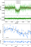 |
Fig. 5 Top: TESS phase-folded transits after subtracting the GP-modelled activity, along with the transit model shown with a black line and the residuals below it. Bottom: HARPS-N phased curve of RV data after subtracting the GP-modelled activity, with the planetary RV model (black line) and the residuals plotted below. The RV error bars are plotted without the jitter, the value of which is reported in Table A.2. |
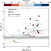 |
Fig. 6 Mass–radius diagram for young (≤1 Gyr) planets with precise age estimates (relative errors <50%). Planets are colour-coded based on their age, with a discrete colour bar at the top of the figure. Young planets with similar characteristics to TOI-5734b are labelled with their name. The Zeng et al. (2019) tracks, shown as dashed lines, are reported in the case of planets with an equilibrium temperature of Teq = 700 K, 1 mbar pressure and the following compositions: 100% Earth-like, 100% H2O, 100% rock (MgSiO3), 50% Earth+50% H2O, 99.9% Earth+0.1% H2 envelope. The wide, horizontal grey line represents the ‘radius valley’. |
6.2 Atmospheric evolution
Since TOI-5734b is a close-in planet orbiting a young star, it is subjected to the high-energy irradiation emitted by its host. This condition could have a strong impact on the atmospheric evolution of such a low-mass planet, whose gravity is unable to retain volatile chemical species heated by the intense stellar radiation. To study the atmospheric photo-evaporation over time, we adopted a modelling approach initially proposed by Locci et al. (2019) that was refined in subsequent works (see, e.g. Mantovan et al. 2024b). In brief, we evaluated the mass–loss rate of the planetary atmosphere by using the analytical approximation derived from the ATES hydrodynamic code (Caldiroli et al. 2021, 2022), coupled with the planetary core-envelope models by Fortney et al. (2007) and Lopez & Fortney (2014), the MESA stellar tracks (MIST; Choi et al. 2016), the X-ray luminosity time evolution by Penz et al. (2008), and the X-ray-to-EUV scaling by Sanz-Forcada et al. (2025). We underline that we use the term ‘core’ to refer specifically to all the solid components of the planet. As a first step, we calculated the planetary structure. Starting from the mass and radius at the current age, we determined the mass and radius of the core, the radius of the gaseous envelope, and the atmospheric mass fraction. To do this, we solved a system of four equations with four unknowns. One equation is from Fortney et al. (2007), which provides the core radius as a function of core mass; another is from Lopez & Fortney (2014), which gives the envelope radius as a function of the atmospheric fraction. Finally, we included two closing equations: one that gives the planetary radius as the sum of the envelope and core radius, and another that calculates the planetary mass as the sum of the core and atmospheric mass. Thus, keeping this planetary structure constant over time, we calculated the mass lost by the planet due to evaporation. We then updated the planetary radius, which changes both due to gravitational contraction and in response to mass loss. Finally, we updated both the bolometric luminosity and the X and EUV luminosities (see Sect. 3.7). Our simulation traces the planet’s evolution back in time to 10 Myr, at which point we assume the stellar disc had dissipated and the planet had reached its final orbit, while the simulation ended at 5 Gyr. To perform simulations of the past and future planetary evolution, we assumed an Earth-like core with a rock–iron (67%, 33%) composition. To compute the planetary radius, we considered solar metallicity (Lopez & Fortney 2014). Figure A.6 shows the values of the core mass, core radius, and atmospheric mass fraction, at the present age, as a function of the planetary radius. We found that the system has a solution for only a very low value of the atmospheric mass fraction. We needed to move to higher values of planetary radii or lower values of the rocky fraction to find a higher value of the atmospheric mass fraction. An ice–rock composition would produce a higher core radius, giving even lower values for the atmospheric mass fraction. However, the system of an ice–rock composition does not find a solution for the nominal values of mass and radius, suggesting that an Earth-like core composition is more appropriate. At the current age, we determined a core mass and a radius of 9.07 M⊕ and 1.75 R⊕, respectively. According to our calculations, the planet has only a small atmospheric fraction, ~0.25%, suggesting that it has likely already lost most of its primordial envelope entirely. We emphasise that this conclusion holds under the assumption of an Earth-like core and a hydrogen-dominated atmosphere. As for the future evolution, we found that the planet will completely lose its primary atmosphere in approximately 300 Myr, and it will end as a Chthonian planet (rocky core remnant of the atmospheric escape process a planet underwent during its evolution; Hébrard et al. 2004), with a radius and mass equivalent to those of the core (unless it develops a secondary atmosphere). We also determined that the planet began its evolution with a mass of ~9.24 M⊕ and a radius of ~3.41 R⊕. In Fig. 7, we show the temporal evolution of some planetary parameters. The figure also shows the evolutions taking into account different ages for the star; in particular, we considered the values of 350 Myr and 800 Myr, i.e. ±1σ with respect to the nominal age. An older age would imply that the planet has undergone the photoevaporation process for a longer time; hence, it would have had a greater mass at 10 Myr. The opposite argument would apply in the case of a younger age. Changing the law used to calculate the mass-loss rate does not alter the planet’s fate, it just changes the timescale needed for the planet to lose its atmosphere. In particular, the timescale is a factor of ~1.8 longer in the case of the formulation proposed by Kubyshkina et al. (2018), because it predicts a lower mass-loss rate with respect to that computed with the analytical formulation of ATES (Caldiroli et al. 2021, 2022). We conclude that, during its lifetime, the planet has likely moved from the region at larger radii in the mass–radius diagram to its current position near the radius gap.
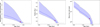 |
Fig. 7 Temporal evolution of mass fraction, radius, and mass-loss rate of TOI-5734b. The panels show the evolution of atmospheric mass fraction (left), radius (middle), and mass-loss rate (right). Solid lines represent the future evolution, whereas dashed lines represent the past one. The grey lines represent the temporal evolution, considering an age equal to ±1σ the nominal age. The red circle shows the position of TOI-5734b at the current age. |
6.3 Orbital evolution
We estimated the timescale of tidal circularisation of the orbit of TOI-5734b. In this system, orbit circularisation is dominated by tides inside the planet. Assuming a modified tidal-quality factor of ![Mathematical equation: $\[Q_{p l}^{\prime}=1000\]$](/articles/aa/full_html/2026/04/aa55931-25/aa55931-25-eq50.png) , which is appropriate for a planet with a rocky internal structure (Lanza 2021), we find a circularisation e-folding timescale e/lde/dtl of 1.1 Gyr, which is comparable with or slightly longer than the age of the system. Therefore, the planet is likely to have formed by migration in a disk rather than through high-eccentricity migration (HEM; Rasio & Ford 1996) followed by circularisation, because the latter scenario would require a time span longer than the age of the system. Moreover, the semi-major axis of the planet is more than ten times larger than the semi-major axis corresponding to the Roche limit (0.0053 au for our target), while in the case of HEM, one would expect a semi-major axis around three times the Roche limit (Ford & Rasio 2006).
, which is appropriate for a planet with a rocky internal structure (Lanza 2021), we find a circularisation e-folding timescale e/lde/dtl of 1.1 Gyr, which is comparable with or slightly longer than the age of the system. Therefore, the planet is likely to have formed by migration in a disk rather than through high-eccentricity migration (HEM; Rasio & Ford 1996) followed by circularisation, because the latter scenario would require a time span longer than the age of the system. Moreover, the semi-major axis of the planet is more than ten times larger than the semi-major axis corresponding to the Roche limit (0.0053 au for our target), while in the case of HEM, one would expect a semi-major axis around three times the Roche limit (Ford & Rasio 2006).
7 Conclusions
In this paper, we present the dynamical mass determination of a planet transiting the active star TOI-5734, first observed with TESS. TOI-5734 is a K3-K4 V star with a Teff of 4750 K. Based on the stellar Prot (~11.09 d), coronal and chromospheric activity, and lithium EW, we find that the star is relatively young, with an age ~500 Myr. We combined the TESS observations with a dataset of RV measurements collected with HARPS-N at TNG to model stellar activity and planetary signal simultaneously. We used a GP regression to extract the activity signal with a dSHO kernel, which modelled the stellar rotational period and its first harmonic. This approach helped us to constrain the stellar and planetary parameters. We tested several models, and we found that TOI-5734 is orbited by a planet with a mass of ~9.1 M⊕ and a radius of ~2.10 R⊕ leading to a density of ~5.4 g/cm3 ~ 0.98 ρ⊕. TOI-5734b is a hot sub-Neptune possibly with a rocky composition and a depleted (almost) primary atmosphere that is located slightly above the upper edge of the ‘radius valley’ in the mass-radius diagram. This is also confirmed by the simulation of the past and future planetary evolution, suggesting that the planet will completely lose its primordial envelope within 300 Myr, ending its evolution as a Chthonian planet. Despite these results, taking into account its mass and radius uncertainties, the planet location is possibly compatible with a water-world model (composition of 50% H2O), which cannot be discarded in the absence of other informative data.
Thanks to the JWST and the future launch of Ariel in 2029, it will be possible to probe the exoplanet atmospheres of young transiting planets and look at the atmospheric composition and the possible presence of clouds and hazes in detail. This will also allow us to obtain insight into the formation and migration mechanisms of young exoplanets. For the particular case of TOI-5734b, we employed the ArielRad radiometric model (Mugnai et al. 2020) to evaluate the number of transits needed to achieve the required S/N to detect the presence of a primary atmosphere during the Ariel Tier 1 observation phase. Assuming a cloud-free atmosphere and the planetary and stellar properties obtained in this work, the number of transits is 19. In particular, the detection of the primary atmosphere for this planet could validate our atmospheric evolution simulations and deepen our knowledge of the evolution of young exoplanetary atmospheres.
Acknowledgements
This work made use of tpfplotter by J. Lillo-Box (publicly available at www.github.com/jlillo/tpfplotter), which also made use of the Python packages astropy, lightkurve, matplotlib and numpy. This research has made use of the Exoplanet Follow-up Observation Programme (ExoFOP; DOI: 10.26134/ExoFOP5) website, which is operated by the California Institute of Technology, under contract with the National Aeronautics and Space Administration under the Exoplanet Exploration Program. This work includes data collected with the TESS mission, obtained from the MAST data archive at the Space Telescope Science Institute (STScI). This work has made use of data from the European Space Agency (ESA) mission Gaia (https://www.cosmos.esa.int/gaia), processed by the Gaia Data Processing and Analysis Consortium (DPAC, https://www.cosmos.esa.int/web/gaia/dpac/consortium). Funding for the DPAC has been provided by national institutions, in particular, the institutions participating in the Gaia Multilateral Agreement. This work makes use of observations from the LCOGT network. Part of the LCOGT telescope time was granted by NOIRLab through the Mid-Scale Innovations Program (MSIP). MSIP is funded by NSF. This work is based on observations obtained at the Hale Telescope, Palomar Observatory, as part of a collaborative agreement between the Caltech Optical Observatories and the Jet Propulsion Laboratory operated by Caltech for NASA. This work has been financially supported by the PRIN-INAF 2019 Planetary systems at young ages (PLATEA), the grant INAF 2022 TRAME@JWST (TRacing the Accretion Metallicity rElationship with NIRSpec@JWST), the ASI-INAF agreement 2021-5-HH.0, the INAF Guest Observer Grant (Large) “GAPS2” and the INAF Guest Observer Grant (Normal) “ArMS: the Ariel Masses Survey Large Program at the TNG”, according to the INAF Fundamental Astrophysics funding scheme. Part of the research activities described in this paper were carried out with contribution of the Next Generation EU funds within the National Recovery and Resilience Plan (PNRR), Mission 4 – Education and Research, Component 2 – From Research to Business (M4C2), Investment Line 3.1 – Strengthening and creation of Research Infrastructures, Project IR0000034 – ‘STILES - Strengthening the Italian Leadership in ELT and SKA’. SF thanks the Max Planck Institute for Astronomy (Heidelberg) for the kind hospitality. T.T. acknowledges support by the BNSF program “VIHREN-2021” project No. KP-06-DV/5. LMan acknowledges financial contribution from PRIN MUR 2022 project 2022J4H55R. IAS acknowledges the support of the MV Lomonosov Moscow State University Program of Development. TZi acknowledges support from the CHEOPS ASI-INAF agreement no. 2019-29-HH.0, NVIDIA Academic Hardware Grant Program for the use of the Titan V GPU card and the Italian MUR Departments of Excellence grant 2023–2027 Quantum Frontiers. DRC acknowledges partial support from NASA Grant 18-2XRP18_2-0007. We acknowledge the Italian centre for Astronomical Archives (IA2, https://www.ia2.inaf.it) for providing technical assistance, services and supporting activities. SF thanks G.S.A. Pallavolo Ariano a.s.d. for its support and wishes to dedicate this work to it.
References
- Adamow, M. M. 2017, in American Astronomical Society Meeting Abstracts, 230, American Astronomical Society Meeting Abstracts #230, 216.07 [Google Scholar]
- Aller, A., Lillo-Box, J., Jones, D., Miranda, L. F., & Barceló Forteza, S. 2020, A&A, 635, A128 [NASA ADS] [CrossRef] [EDP Sciences] [Google Scholar]
- Baliunas, S. L., Donahue, R. A., Soon, W. H., et al. 1995, ApJ, 438, 269 [Google Scholar]
- Baratella, M., D’Orazi, V., Biazzo, K., et al. 2020a, A&A, 640, A123 [NASA ADS] [CrossRef] [EDP Sciences] [Google Scholar]
- Baratella, M., D’Orazi, V., Carraro, G., et al. 2020b, A&A, 634, A34 [NASA ADS] [CrossRef] [EDP Sciences] [Google Scholar]
- Barragán, O., Armstrong, D. J., Gandolfi, D., et al. 2022, MNRAS, 514, 1606 [CrossRef] [Google Scholar]
- Benatti, S., Nardiello, D., Malavolta, L., et al. 2019, A&A, 630, A81 [NASA ADS] [CrossRef] [EDP Sciences] [Google Scholar]
- Benatti, S., Damasso, M., Borsa, F., et al. 2021, A&A, 650, A66 [NASA ADS] [CrossRef] [EDP Sciences] [Google Scholar]
- Biazzo, K., D’Orazi, V., Desidera, S., et al. 2022, A&A, 664, A161 [NASA ADS] [CrossRef] [EDP Sciences] [Google Scholar]
- Bonomo, A. S., Dumusque, X., Massa, A., et al. 2023, A&A, 677, A33 [NASA ADS] [CrossRef] [EDP Sciences] [Google Scholar]
- Bonomo, A., Borsato, L., Rajpaul, V. M., et al. 2025, A&A, 696, A233 [NASA ADS] [CrossRef] [EDP Sciences] [Google Scholar]
- Boss, A. P. 1997, Science, 276, 1836 [Google Scholar]
- Brown, T. M., Baliber, N., Bianco, F. B., et al. 2013, PASP, 125, 1031 [Google Scholar]
- Burn, R., Mordasini, C., Mishra, L., et al. 2024, Nat. Astron., 8, 463 [Google Scholar]
- Caldiroli, A., Haardt, F., Gallo, E., et al. 2021, A&A, 655, A30 [NASA ADS] [CrossRef] [EDP Sciences] [Google Scholar]
- Caldiroli, A., Haardt, F., Gallo, E., et al. 2022, A&A, 663, A122 [NASA ADS] [CrossRef] [EDP Sciences] [Google Scholar]
- Cale, B. L., Reefe, M., Plavchan, P., et al. 2021, AJ, 162, 295 [NASA ADS] [CrossRef] [Google Scholar]
- Carleo, I., Malavolta, L., Lanza, A. F., et al. 2020, A&A, 638, A5 [NASA ADS] [CrossRef] [EDP Sciences] [Google Scholar]
- Carleo, I., Desidera, S., Nardiello, D., et al. 2021, A&A, 645, A71 [EDP Sciences] [Google Scholar]
- Casagrande, L., Lin, J., Rains, A. D., et al. 2021, MNRAS, 507, 2684 [NASA ADS] [CrossRef] [Google Scholar]
- Castelli, F., & Kurucz, R. L. 2003, in Modelling of Stellar Atmospheres, 210, eds. N. Piskunov, W. W. Weiss, & D. F. Gray, A20 [Google Scholar]
- Choi, J., Dotter, A., Conroy, C., et al. 2016, ApJ, 823, 102 [Google Scholar]
- Ciardi, D. R., Beichman, C. A., Horch, E. P., & Howell, S. B. 2015, ApJ, 805, 16 [NASA ADS] [CrossRef] [Google Scholar]
- Claret, A. 2018, A&A, 618, A20 [NASA ADS] [CrossRef] [EDP Sciences] [Google Scholar]
- Collins, K. 2019, in American Astronomical Society Meeting Abstracts, 233, American Astronomical Society Meeting Abstracts #233, 140.05 [Google Scholar]
- Collins, K. A., Kielkopf, J. F., Stassun, K. G., & Hessman, F. V. 2017, AJ, 153, 77 [Google Scholar]
- Cosentino, R., Lovis, C., Pepe, F., et al. 2014, in Ground-based and Airborne Instrumentation for Astronomy V, 9147, SPIE, 2658 [Google Scholar]
- Covino, E., Esposito, M., Barbieri, M., et al. 2013, A&A, 554, A28 [NASA ADS] [CrossRef] [EDP Sciences] [Google Scholar]
- Currie, T., Lawson, K., Schneider, G., et al. 2022, Nat. Astron., 6, 751 [NASA ADS] [CrossRef] [Google Scholar]
- Curtis, J. L., Agüeros, M. A., Matt, S. P., et al. 2020, ApJ, 904, 140 [Google Scholar]
- Cutri, R. M., Skrutskie, M. F., van Dyk, S., et al. 2003, 2MASS All Sky Catalog of point sources [Google Scholar]
- da Silva, L., Girardi, L., Pasquini, L., et al. 2006, A&A, 458, 609 [NASA ADS] [CrossRef] [EDP Sciences] [Google Scholar]
- Damasso, M., Locci, D., Benatti, S., et al. 2023, A&A, 672, A126 [NASA ADS] [CrossRef] [EDP Sciences] [Google Scholar]
- Dekany, R., Roberts, J., Burruss, R., et al. 2013, ApJ, 776, 130 [CrossRef] [Google Scholar]
- Desidera, S., Covino, E., Messina, S., et al. 2015, A&A, 573, A126 [NASA ADS] [CrossRef] [EDP Sciences] [Google Scholar]
- Desidera, S., Damasso, M., Gratton, R., et al. 2023, A&A, 675, A158 [NASA ADS] [CrossRef] [EDP Sciences] [Google Scholar]
- Dutra-Ferreira, L., Pasquini, L., Smiljanic, R., Porto de Mello, G. F., & Steffen, M. 2016, A&A, 585, A75 [NASA ADS] [CrossRef] [EDP Sciences] [Google Scholar]
- Eastman, J., Gaudi, B. S., & Agol, E. 2013, PASP, 125, 83 [Google Scholar]
- Espinoza, N., Kossakowski, D., & Brahm, R. 2019, MNRAS, 490, 2262 [Google Scholar]
- Evans, I. N., Primini, F. A., Glotfelty, K. J., et al. 2010, ApJS, 189, 37 [NASA ADS] [CrossRef] [Google Scholar]
- Filomeno, S., Biazzo, K., Baratella, M., et al. 2024, A&A, 690, A370 [NASA ADS] [CrossRef] [EDP Sciences] [Google Scholar]
- Ford, E. B., & Rasio, F. A. 2006, ApJ, 638, L45 [Google Scholar]
- Foreman-Mackey, D. 2018, RNAAS, 2, 31 [NASA ADS] [Google Scholar]
- Foreman-Mackey, D., Agol, E., Ambikasaran, S., & Angus, R. 2017, AJ, 154, 220 [Google Scholar]
- Fortney, J. J., Marley, M. S., & Barnes, J. W. 2007, ApJ, 659, 1661 [Google Scholar]
- Fulton, B. J., & Petigura, E. A. 2018, AJ, 156, 264 [Google Scholar]
- Fulton, B. J., Petigura, E. A., Howard, A. W., et al. 2017, AJ, 154, 109 [Google Scholar]
- Furlan, E., Ciardi, D. R., Everett, M. E., et al. 2017, AJ, 153, 71 [NASA ADS] [CrossRef] [Google Scholar]
- Gagné, J., Mamajek, E. E., Malo, L., et al. 2018, ApJ, 856, 23 [Google Scholar]
- Gaia Collaboration (Prusti, T., et al.) 2016, A&A, 595, A1 [NASA ADS] [CrossRef] [EDP Sciences] [Google Scholar]
- Gaia Collaboration (Vallenari, A., et al.) 2023, A&A, 674, A1 [NASA ADS] [CrossRef] [EDP Sciences] [Google Scholar]
- Giacalone, S., Dressing, C. D., Jensen, E. L. N., et al. 2021, AJ, 161, 24 [Google Scholar]
- Hayward, T. L., Brandl, B., Pirger, B., et al. 2001, PASP, 113, 105 [NASA ADS] [CrossRef] [Google Scholar]
- Hébrard, G., Lecavelier Des Étangs, A., Vidal-Madjar, A., Désert, J. M., & Ferlet, R. 2004, in Astronomical Society of the Pacific Conference Series, 321, Extrasolar Planets: Today and Tomorrow, eds. J. Beaulieu, A. Lecavelier Des Etangs, & C. Terquem, 203 [Google Scholar]
- Hippke, M., & Heller, R. 2019, A&A, 623, A39 [NASA ADS] [CrossRef] [EDP Sciences] [Google Scholar]
- Hippke, M., David, T. J., Mulders, G. D., & Heller, R. 2019, AJ, 158, 143 [Google Scholar]
- Howell, S. B., Everett, M. E., Sherry, W., Horch, E., & Ciardi, D. R. 2011, AJ, 142, 19 [Google Scholar]
- Husser, T., Wende-von Berg, S., Dreizler, S., et al. 2013, A&A, 553, A6 [NASA ADS] [CrossRef] [EDP Sciences] [Google Scholar]
- Ida, S., & Lin, D. N. C. 2004, ApJ, 604, 388 [Google Scholar]
- Jeffries, R. D., Jackson, R. J., Wright, N. J., et al. 2023, MNRAS, 523, 802 [NASA ADS] [CrossRef] [Google Scholar]
- Jenkins, J. M., Twicken, J. D., McCauliff, S., et al. 2016, in SPIE Conference Series, 9913, Software and Cyberinfrastructure for Astronomy IV, eds. G. Chiozzi, & J. C. Guzman, 99133E [Google Scholar]
- Johnson, D. R. H., & Soderblom, D. R. 1987, AJ, 93, 864 [Google Scholar]
- Kaltenegger, L., & Sasselov, D. 2011, ApJ, 736, L25 [Google Scholar]
- Kipping, D. M. 2013, MNRAS, 435, 2152 [Google Scholar]
- Kreidberg, L. 2015, PASP, 127, 1161 [Google Scholar]
- Kubyshkina, D., Fossati, L., Erkaev, N. V., et al. 2018, ApJ, 866, L18 [NASA ADS] [CrossRef] [Google Scholar]
- Lallement, R., Capitanio, L., Ruiz-Dern, L., et al. 2018, A&A, 616, A132 [NASA ADS] [CrossRef] [EDP Sciences] [Google Scholar]
- Lanza, A. F. 2021, A&A, 653, A112 [NASA ADS] [CrossRef] [EDP Sciences] [Google Scholar]
- Lanza, A. F., Bonomo, A. S., Moutou, C., et al. 2010, A&A, 520, A53 [NASA ADS] [CrossRef] [EDP Sciences] [Google Scholar]
- Lind, K., Asplund, M., & Barklem, P. S. 2009, A&A, 503, 541 [NASA ADS] [CrossRef] [EDP Sciences] [Google Scholar]
- Lindegren, L., Hernández, J., Bombrun, A., et al. 2018, A&A, 616, A2 [NASA ADS] [CrossRef] [EDP Sciences] [Google Scholar]
- Lindegren, L., Klioner, S. A., Hernández, J., et al. 2021, A&A, 649, A2 [EDP Sciences] [Google Scholar]
- Locci, D., Cecchi-Pestellini, C., & Micela, G. 2019, A&A, 624, A101 [NASA ADS] [CrossRef] [EDP Sciences] [Google Scholar]
- Lopez, E. D., & Fortney, J. J. 2014, ApJ, 792, 1 [Google Scholar]
- Lovis, C., Dumusque, X., Santos, N. C., et al. 2011, arXiv e-prints [arXiv:1107.5325] [Google Scholar]
- Luque, R., & Pallé, E. 2022, Science, 377, 1211 [NASA ADS] [CrossRef] [Google Scholar]
- Mallorquín, M., Béjar, V. J. S., Lodieu, N., et al. 2023, A&A, 671, A163 [NASA ADS] [CrossRef] [EDP Sciences] [Google Scholar]
- Mamajek, E. E., & Hillenbrand, L. A. 2008, ApJ, 687, 1264 [Google Scholar]
- Mantovan, G., Malavolta, L., Desidera, S., et al. 2024a, A&A, 682, A129 [NASA ADS] [CrossRef] [EDP Sciences] [Google Scholar]
- Mantovan, G., Malavolta, L., Locci, D., et al. 2024b, A&A, 684, L17 [NASA ADS] [CrossRef] [EDP Sciences] [Google Scholar]
- Matsuo, T., Shibai, H., Ootsubo, T., & Tamura, M. 2007, ApJ, 662, 1282 [NASA ADS] [CrossRef] [Google Scholar]
- Maxted, P. F. L. 2018, A&A, 616, A39 [NASA ADS] [CrossRef] [EDP Sciences] [Google Scholar]
- McCully, C., Volgenau, N. H., Harbeck, D.-R., et al. 2018, SPIE Conf. Ser., 10707, 107070K [Google Scholar]
- Merloni, A., Lamer, G., Liu, T., et al. 2024, A&A, 682, A34 [NASA ADS] [CrossRef] [EDP Sciences] [Google Scholar]
- Montes, D., López-Santiago, J., Gálvez, M. C., et al. 2001, MNRAS, 328, 45 [NASA ADS] [CrossRef] [Google Scholar]
- Mugnai, L. V., Pascale, E., Edwards, B., Papageorgiou, A., & Sarkar, S. 2020, Exp. Astron., 50, 303 [NASA ADS] [CrossRef] [Google Scholar]
- Müller, S., Baron, J., Helled, R., Bouchy, F., & Parc, L. 2024, A&A, 686, A296 [NASA ADS] [CrossRef] [EDP Sciences] [Google Scholar]
- Naponiello, L., Bonomo, A. S., Mancini, L., et al. 2025, A&A, 693, A7 [NASA ADS] [CrossRef] [EDP Sciences] [Google Scholar]
- Nardiello, D. 2020, MNRAS, 498, 5972 [Google Scholar]
- Nardiello, D., Borsato, L., Piotto, G., et al. 2019, MNRAS, 490, 3806 [NASA ADS] [CrossRef] [Google Scholar]
- Nardiello, D., Piotto, G., Deleuil, M., et al. 2020, MNRAS, 495, 4924 [Google Scholar]
- Nardiello, D., Deleuil, M., Mantovan, G., et al. 2021, MNRAS, 505, 3767 [NASA ADS] [CrossRef] [Google Scholar]
- Nardiello, D., Malavolta, L., Desidera, S., et al. 2022, A&A, 664, A163 [NASA ADS] [CrossRef] [EDP Sciences] [Google Scholar]
- Nardiello, D., Akana Murphy, J. M., Spinelli, R., et al. 2025, A&A, 693, A32 [NASA ADS] [CrossRef] [EDP Sciences] [Google Scholar]
- Newton, E. R., Mann, A. W., Tofflemire, B. M., et al. 2019, ApJ, 880, L17 [Google Scholar]
- Paegert, M., Stassun, K. G., Collins, K. A., et al. 2022, VizieR Online Data Catalog: IV/39 [Google Scholar]
- Patel, J. A., & Espinoza, N. 2022, AJ, 163, 228 [NASA ADS] [CrossRef] [Google Scholar]
- Pecaut, M. J., & Mamajek, E. E. 2013, ApJS, 208, 9 [Google Scholar]
- Penz, T., Micela, G., & Lammer, H. 2008, A&A, 477, 309 [NASA ADS] [CrossRef] [EDP Sciences] [Google Scholar]
- Petigura, E. A., Rogers, J. G., Isaacson, H., et al. 2022, AJ, 163, 179 [NASA ADS] [CrossRef] [Google Scholar]
- Piaulet-Ghorayeb, C., Benneke, B., Radica, M., et al. 2024, ApJ, 974, L10 [NASA ADS] [CrossRef] [Google Scholar]
- Pizzolato, N., Maggio, A., Micela, G., Sciortino, S., & Ventura, P. 2003, A&A, 397, 147 [NASA ADS] [CrossRef] [EDP Sciences] [Google Scholar]
- Psaridi, A., Osborn, H., Bouchy, F., et al. 2024, A&A, 685, A5 [NASA ADS] [CrossRef] [EDP Sciences] [Google Scholar]
- Rainer, M., Desidera, S., Borsa, F., et al. 2023, A&A, 676, A90 [NASA ADS] [CrossRef] [EDP Sciences] [Google Scholar]
- Rasio, F. A., & Ford, E. B. 1996, Science, 274, 954 [Google Scholar]
- Rasmussen, C. E., & Williams, C. K. I. 2006, Gaussian Processes for Machine Learning (The MIT Press) [Google Scholar]
- Ricker, G. R., Winn, J. N., Vanderspek, R., et al. 2014, SPIE Conf. Ser., 9143, 914320 [Google Scholar]
- Sanz-Forcada, J., López-Puertas, M., Lampón, M., et al. 2025, A&A, 693, A285 [NASA ADS] [CrossRef] [EDP Sciences] [Google Scholar]
- Schlegel, D. J., Finkbeiner, D. P., & Davis, M. 1998, ApJ, 500, 525 [Google Scholar]
- Scott, N. J., Howell, S. B., Horch, E. P., & Everett, M. E. 2018, PASP, 130, 054502 [Google Scholar]
- Sneden, C. 1973, ApJ, 184, 839 [Google Scholar]
- Sousa, S. G., Santos, N. C., Adibekyan, V., Delgado-Mena, E., & Israelian, G. 2015, A&A, 577, A67 [NASA ADS] [CrossRef] [EDP Sciences] [Google Scholar]
- Sozzetti, A. 2023, A&A, 670, L17 [NASA ADS] [CrossRef] [EDP Sciences] [Google Scholar]
- Speagle, J. S. 2020, MNRAS, 493, 3132 [Google Scholar]
- Spiegel, D. S., Fortney, J. J., & Sotin, C. 2014, PNAS, 111, 12622 [NASA ADS] [CrossRef] [Google Scholar]
- Stassun, K. G., & Torres, G. 2016, ApJ, 831, L6 [NASA ADS] [CrossRef] [Google Scholar]
- Stassun, K. G., & Torres, G. 2018, ApJ, 862, 61 [Google Scholar]
- Stassun, K. G., & Torres, G. 2021, ApJ, 907, L33 [NASA ADS] [CrossRef] [Google Scholar]
- Stassun, K. G., Collins, K. A., & Gaudi, B. S. 2017, AJ, 153, 136 [Google Scholar]
- Strakhov, I. A., Safonov, B. S., & Cheryasov, D. V. 2023, Astrophys. Bull., 78, 234 [NASA ADS] [CrossRef] [Google Scholar]
- Sun, L., Ioannidis, P., Gu, S., et al. 2019, A&A, 624, A15 [NASA ADS] [CrossRef] [EDP Sciences] [Google Scholar]
- Tinetti, G., Drossart, P., Eccleston, P., et al. 2018, Exp. Astron., 46, 135 [NASA ADS] [CrossRef] [Google Scholar]
- Torres, G. 2010, AJ, 140, 1158 [Google Scholar]
- Trifonov, T. 2019, The Exo-Striker: Transit and radial velocity interactive fitting tool for orbital analysis and N-body simulations, Astrophysics Source Code Library [record ascl:1906.004] [Google Scholar]
- Trotta, R. 2008, Contemp. Phys., 49, 71 [Google Scholar]
- Tychoniec, Ł., Manara, C. F., Rosotti, G. P., et al. 2020, A&A, 640, A19 [NASA ADS] [CrossRef] [EDP Sciences] [Google Scholar]
- Van Eylen, V., Agentoft, C., Lundkvist, M. S., et al. 2018, MNRAS, 479, 4786 [Google Scholar]
- Zechmeister, M., & Kürster, M. 2009, A&A, 496, 577 [CrossRef] [EDP Sciences] [Google Scholar]
- Zechmeister, M., Reiners, A., Amado, P. J., et al. 2018, A&A, 609, A12 [NASA ADS] [CrossRef] [EDP Sciences] [Google Scholar]
- Zeng, L., Jacobsen, S. B., Sasselov, D. D., et al. 2019, PNAS, 116, 9723 [Google Scholar]
The S-index was measured from the Ca II H&K emission using the code from Alejandro Suarez Mascareno and Christophe Lovis.
NOIRLab IRAF is distributed by the Community Science and Data Center at NSF NOIRLab, which is managed by the Association of Universities for Research in Astronomy (AURA) under a cooperative agreement with the U.S. National Science Foundation.
Appendix A Additional tables and figures
The study exploited the light curves from three TESS sectors (20, 47, 60). We checked that the detected transits originate on our target and are not associated with a neighbour source using the procedure in Nardiello et al. (2020). This was done by looking at the differences between the mean in- and out-of-transit centroids of each sector, where the centroid and the target (at (0,0) coordinates) show compatible positions, within the errors, as reported in Fig. A.1. The analysis was conducted with spectroscopic data extracted from 97 HARPS-N high-resolution spectra. The time series of RVs and the BIS span, and ![Mathematical equation: $\[\log~ R_{\mathrm{HK}}^{\prime}\]$](/articles/aa/full_html/2026/04/aa55931-25/aa55931-25-eq51.png) activity indices are tabulated in Table A.1 and displayed in Fig. A.2. The bottom panel of Fig. A.2 shows an increasing trend of the
activity indices are tabulated in Table A.1 and displayed in Fig. A.2. The bottom panel of Fig. A.2 shows an increasing trend of the ![Mathematical equation: $\[\log~ R_{\mathrm{HK}}^{\prime}\]$](/articles/aa/full_html/2026/04/aa55931-25/aa55931-25-eq52.png) . This trend implies a higher level of activity variability in the second observational season, which leads to more scattered radial-velocity measurements as shown in the top panel of Fig. A.2. Fig. A.3 shows the RV time series fitted with the GP model activity component after subtracting the planetary signal. As shown in the figure, the higher scattering of RV data in the second observational season is completely absorbed by the GP model. The best fit parameters of our simultaneous RV and light curve model with the GP hyperparameters used to remove the stellar contribution are presented in the corner plots of Fig. A.4 and Fig. A.5, showing respectively the posterior distribution of the main planetary parameters and that of the global fit data, such as jitter, GP hyperparameters and LDC, each with the 1 σ, 2 σ, and 3 σ confidence levels. Nested sampling priors and posteriors (median and the 16th and 84th percentiles) of the GP hyperparameters and the other system parameters used in the analysis are reported in Table A.2. Following the discussion on atmospheric evolution simulations in Sect. 6.2, we report in Figure A.6 the solutions of the core-envelope model assuming a rock-iron core composition, where the core mass, core radius, and atmospheric mass fraction, at the present age, are plotted as a function of the planetary radius.
. This trend implies a higher level of activity variability in the second observational season, which leads to more scattered radial-velocity measurements as shown in the top panel of Fig. A.2. Fig. A.3 shows the RV time series fitted with the GP model activity component after subtracting the planetary signal. As shown in the figure, the higher scattering of RV data in the second observational season is completely absorbed by the GP model. The best fit parameters of our simultaneous RV and light curve model with the GP hyperparameters used to remove the stellar contribution are presented in the corner plots of Fig. A.4 and Fig. A.5, showing respectively the posterior distribution of the main planetary parameters and that of the global fit data, such as jitter, GP hyperparameters and LDC, each with the 1 σ, 2 σ, and 3 σ confidence levels. Nested sampling priors and posteriors (median and the 16th and 84th percentiles) of the GP hyperparameters and the other system parameters used in the analysis are reported in Table A.2. Following the discussion on atmospheric evolution simulations in Sect. 6.2, we report in Figure A.6 the solutions of the core-envelope model assuming a rock-iron core composition, where the core mass, core radius, and atmospheric mass fraction, at the present age, are plotted as a function of the planetary radius.
 |
Fig. A.1 In- and out-of-transit centroid of TOI-5734. Within the errors, the centroid coordinates coincide with the target position (located in (0,0)). |
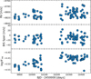 |
Fig. A.2 HARPS-N spectroscopic time series used in this work. From top to bottom, the RV, the BIS span and the |
![Mathematical equation: $\[\log~ R_{\mathrm{HK}}^{\prime}\]$](/articles/aa/full_html/2026/04/aa55931-25/aa55931-25-eq53.png)
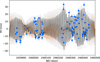 |
Fig. A.3 RV data with the GP model component after subtracting the planetary component. |
Time series of TOI-5734 from HARPS-N data showing Barycentric Julian Dates (BJD), radial velocities (RV) with uncertainties and the BIS span and ![Mathematical equation: $\[R_{\mathrm{HK}}^{\prime}\]$](/articles/aa/full_html/2026/04/aa55931-25/aa55931-25-eq54.png) activity indices with their uncertainties.
activity indices with their uncertainties.
Nested sampling priors and posteriors (median and the 16th and 84th percentiles) of the GP hyperparameters and the other system parameters used in the analysis of TOI-5734b.
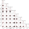 |
Fig. A.4 Corner plot of the posterior distribution of the main planetary parameters resulting from the TESS and HARPS-N analysis done with a NS scheme for TOI-5734b. The dark contours on the panels represent the 1σ, 2σ, and 3σ confidence levels of the overall NS. The red line represents the median value of the posterior distribution (the mode in the case of ib). |
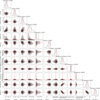 |
Fig. A.5 Corner plot of the posterior distribution of the global data resulting from the TESS and HARPS-N analysis with the GP rotational kernel for TOI-5734b. The dark contours on the panels represent the 1σ, 2σ, and 3σ confidence levels of the overall NS. The red line represents the median value of the posterior distribution. |
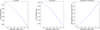 |
Fig. A.6 Solutions of core-envelope models for planet TOI-5734b with total mass fixed at the measured value, considering rock-iron core composition with solar metallicity. The left panel shows the core mass versus the planetary radius, the middle panel shows the core radius, and the right panel shows the atmospheric mass fraction. The purple circle shows the position in the diagram of TOI-5734b at the current age. |
Appendix B Spectral energy distribution analysis
As an independent determination of the basic stellar parameters, we performed an analysis of the broadband SED of the star together with the Gaia DR3 parallax (with no systematic offset applied; see, e.g. Stassun & Torres 2021), to determine an empirical measurement of the stellar radius, following the procedures described in Stassun & Torres (2016); Stassun et al. (2017); Stassun & Torres (2018). We pulled the JHKS magnitudes from 2 MASS, the GBP − GRP magnitudes from Gaia, and the W1–W4 magnitudes from WISE. Together, the available photometry spans the full stellar SED over the wavelength range 0.2–20 μm (see Fig. B.1).
We performed a fit using PHOENIX stellar atmosphere models (Husser et al. 2013), with the Teff, log g, and [Fe/H]adopted from the spectroscopic analysis. The extinction, AV, was limited to the maximum line-of-sight value from the Galactic dust maps of Schlegel et al. (1998). The resulting fit (see Fig. B.1) has a reduced χ2 of 1.2, with a best-fit AV = 0.13 ± 0.03. Integrating the (unreddened) model SED gives the bolometric flux at Earth, Fbol = 6.370 ± 0.074 × 10⁻⁹ erg s−1 cm−2. Taking the Fbol together with the Gaia parallax directly gives the bolometric luminosity, Lbol = 0.2107 ± 0.0024 L⊙. The stellar radius follows from the Stefan-Boltzmann relation, giving R⋆ = 0.678 ± 0.029 R⊙. In addition, we can estimate the stellar mass from the empirical relations of Torres (2010), giving M⋆ = 0.725 ± 0.044 M⊙. The stellar mass and radius estimates obtained through the analysis conducted in this section are similar to the ones found in Sec. 3.7.
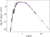 |
Fig. B.1 Spectral energy distribution of TOI-5734. Red symbols represent the observed photometric measurements, where the horizontal bars represent the effective width of the passband. Blue symbols are the model fluxes from the best-fit PHOENIX atmosphere model (black). |
Appendix C LCOGT Ground-based Photometry
The TESS pixel scale is ~21″/pixel and photometric apertures typically extend out to roughly 1 arcminute, generally causing multiple stars to blend in the TESS photometric aperture. To attempt to determine the true source of the TESS detection, we acquired ground-based time series follow-up photometry of the field around TOI-5734 as part of the TESS Follow-up Observing Program (TFOP; Collins 2019)8.
We observed a full transit window of TOI-5734b on UTC 2023 December 11 in Pan-STARRS zs band from the Las Cumbres Observatory Global Telescope (LCOGT) (Brown et al. 2013) 1 m network node at Teide Observatory on the island of Tenerife (TEID). The 1 m telescope is equipped with a 4096 × 4096 px camera having an image scale of ![Mathematical equation: $\[0^{\prime\prime}_\cdot389\]$](/articles/aa/full_html/2026/04/aa55931-25/aa55931-25-eq76.png) per pixel, resulting in a 26′ × 26′ field of view. The images were calibrated by the standard LCOGT BANZAI pipeline (McCully et al. 2018) and differential photometric data were extracted using AstroImageJ (Collins et al. 2017). We used circular
per pixel, resulting in a 26′ × 26′ field of view. The images were calibrated by the standard LCOGT BANZAI pipeline (McCully et al. 2018) and differential photometric data were extracted using AstroImageJ (Collins et al. 2017). We used circular ![Mathematical equation: $\[8^{\prime\prime}_\cdot1\]$](/articles/aa/full_html/2026/04/aa55931-25/aa55931-25-eq77.png) photometric apertures that excluded all flux from all known Gaia DR3 catalogue neighbours. The ingress window was marred by passing clouds. With the weather-affected data removed, we ruled out deep events that could be responsible for the TESS detection in all neighbouring Gaia DR3 stars within 2′.5 of TOI-5734, and detected an on-time 1 ppt egress in the target star aperture, which confirms that the TESS-detected event is indeed occurring on-target. The LCOGT light curve is shown in Figure C.1.
photometric apertures that excluded all flux from all known Gaia DR3 catalogue neighbours. The ingress window was marred by passing clouds. With the weather-affected data removed, we ruled out deep events that could be responsible for the TESS detection in all neighbouring Gaia DR3 stars within 2′.5 of TOI-5734, and detected an on-time 1 ppt egress in the target star aperture, which confirms that the TESS-detected event is indeed occurring on-target. The LCOGT light curve is shown in Figure C.1.
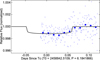 |
Fig. C.1 LCOGT 1 m light curve of TOI-5734b phase folded to the ephemeris reported in this work. The larger blue symbols show the LCOGT data in 18-minute bins. The smaller blue symbols show the unbinned data. An independent transit model fit to the light curve, including ephemeris priors, and fixed a/R* and impact parameters from the global fit in this work, is overplotted using a solid black line. No detrending has been applied since our BIC test preferred an undetrended light curve model. The model has Rp/R* = 0.032 ± 0.004, which is 1σ consistent with the value from the global fit in this work, and Tc = 2460289.6098 ± 0.005 BJD, which is within 1σ consistent with the value predicted by the global fit ephemeris from this work. |
Appendix D High Resolution Imaging
As part of our standard process for validating transiting exoplanets to assess the possible contamination of bound or unbound companions on the derived planetary radii (Ciardi et al. 2015), we observed TOI-5734 with near-infrared adaptive optics imaging on Palomar and optical speckle imaging at WIYN and SAI. The near-infrared and optical imaging complement each other with differing resolutions and sensitivities.
Appendix D.1 Palomar NIR AO Imaging
Observations of TOI-5734 were made on November 27th, 2023, with the PHARO instrument (Hayward et al. 2001) on the Palomar Hale (5 m) behind the P3K natural guide star AO system (Dekany et al. 2013). The pixel scale for PHARO is 0.025″. The Palomar data were collected in a standard 5-point quincunx dither pattern in the Kcont filter. The reduced science frames were combined into a single mosaicked image with final resolutions of ~0.098″.
The sensitivity of the final combined AO images was determined by injecting simulated sources azimuthally around the primary target every 20° at separations of integer multiples of the central source’s FWHM (Furlan et al. 2017). The brightness of each injected source was scaled until standard aperture photometry detected it with 5σ significance. The final 5σ limit at each separation was determined from the average of all of the determined limits at that separation, and the uncertainty on the limit was set by the rms dispersion of the azimuthal slices at a given radial distance. No stellar companions were detected. The 5σ sensitivity as a function of angular separation from TOI-5734 is shown in Figure D.1.
Appendix D.2 WIYN Speckle Imaging
TOI-5734 was observed on February 18th, 2024, using the NN-EXPLORE Exoplanet Stellar Speckle Imager (NESSI; Scott et al. 2018) at the WIYN 3.5 m telescope on Kitt Peak. NESSI data were taken simultaneously in two filters having central wavelengths of λc = 562 and 832 nm and consisted of 9000 40 ms exposures in a 256 × 256 pixel (4.6 × 4.6 arcsec) section of the detectors. A nearby single star was also observed right before the science target to serve as a measure of the point spread function. The NESSI data reduction followed the description given in Howell et al. (2011) and resulted in reconstructed images of the field and contrast curves measured from those images (see Figure D.2). No companion sources were detected near TOI-5734.
Appendix D.3 SAI Speckle Imaging
TOI-5734 was observed on November 8th, 2022, with the speckle polarimeter on the 2.5-m telescope at the Caucasian Observatory of the Sternberg Astronomical Institute (SAI) of Lomonosov Moscow State University. A low-noise CMOS detector, Hamamatsu ORCA-quest (Strakhov et al. 2023), was used as a detector. The atmospheric dispersion compensator was active and allowed the use of the Ic band. The respective angular resolution is 0.083″ and the long-exposure atmospheric seeing was 0.64″. The power spectrum was estimated from 5200 frames with 23 ms of exposure. The contrast detection limits expressed in units of magnitude difference between the source and the potential companion at angular separations 0.25″ and 1.0″ from the star are ΔIc = 4.4 mag and 7.5 mag, respectively. From the acquired data, no companions were detected. The 5σ sensitivity as a function of angular separation from TOI-5734 is shown in Figure D.3.
 |
Fig. D.1 Palomar NIR AO imaging and 5σ sensitivity curve in the Kcont filter. Inset: Image of the central portion of the frames. |
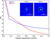 |
Fig. D.2 Contrast curves measured from NESSI at the WIYN 3.5 m telescope for images taken with λc = 562 (blue curve) and 832 nm (red curve) and filters. Inset: Image of the central portion of the frames in the two filters. |
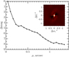 |
Fig. D.3 SAI speckle imaging and contrast curve in the Ic band. Inset: Image of the central portion of the frames. |
Appendix E RV completeness analysis
We estimated the completeness of our RV time series by performing injection-recovery simulations, following Bonomo et al. (2023) and Naponiello et al. (2025). In summary, we injected synthetic RVs with planetary signals at the time of our observations using HARPS-N error bars in addition to the stellar jitter. The signals of additional companions were simulated across a logarithmic 30 × 30 grid in planetary mass (Mp) and semi-major axis (a), covering the ranges [0.01,20] MJup and [0.01,10] au. For each location of the grid, we generated 200 synthetic planetary signals with a free orbital inclination. Then we fitted the signals by employing either Keplerian orbits or linear and quadratic trends to take into account long-period signals. Finally, we adopted the Bayesian information criterion (BIC) to compare the fitted planetary model with a constant model. We considered the planetary signal significantly detected only when ΔBIC > 10 in favour of the planet-induced one. The detection fraction was finally computed as the portion of detected signals for each grid element, as illustrated by Fig. E.1. From this result, we can tell that, with the current dataset, there are no planets of Jovian mass up to 3 au; otherwise, they should have been seen through RV analysis. Jupiter and Saturn have been plotted as a comparison, and they would be at the detection limit and off-limits, respectively.
Furthermore, data from Gaia DR3 for TOI-5734 indicate a RUWE of 0.93. RUWE serves as an indicator of how well a single-star astrometric solution fits the data, and values below 1.4 are generally interpreted as consistent with a good single-star model (see, e.g. Lindegren et al. 2018, 2021). By performing a Monte Carlo analysis to evaluate which combinations of companion mass and orbital separation would lead to RUWE values exceeding those observed in DR3 (following the methodology of Sozzetti 2023), we determined that the Gaia DR3 astrometry rules out, at a 99% confidence level, the presence of companions with masses around 6 times that of Jupiter at separations between approximately 1 and 2.5 au (see Fig. E.2). While RV measurements impose more stringent limits, it’s worth noting that Gaia DR3 astrometry is nearly immune to inclination-related uncertainties.
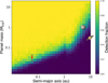 |
Fig. E.1 HARPS-N RV detection map for TOI-5734. The colour scale expresses the detection fraction, while the red circle marks the position of TOI-5734b. Jupiter and Saturn have been plotted as a comparison. |
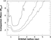 |
Fig. E.2 Sensitivity of Gaia DR3 astrometry. The plot of companion mass vs. orbital radius is based on simulations of planetary signals that would have produced a RUWE value in excess with respect to the one reported in the Gaia DR3 archive. Dashed contours represent the 80%, 90%, and 99% probability, from the outer to the inner. |
All Tables
Nested sampling priors and posteriors (median and the 16th and 84th percentiles) of TOI-5734b orbital parameters.
Comparison between joint fit models where the logarithm of the Bayesian evidence log Z was derived from the NS runs with the 1D–GP activity modelling.
Time series of TOI-5734 from HARPS-N data showing Barycentric Julian Dates (BJD), radial velocities (RV) with uncertainties and the BIS span and activity indices with their uncertainties.
Nested sampling priors and posteriors (median and the 16th and 84th percentiles) of the GP hyperparameters and the other system parameters used in the analysis of TOI-5734b.
All Figures
|
Fig. 1 TESS target pixel file of Sector 20 of TOI-5734, which is marked with ‘1’. The other sources, extracted from the Gaia DR3 catalogue, have numbered circles of sizes proportional to the G-mag difference with our target. The colour bar shows the electron counts for each pixel. The orange squares represent the pixels used to construct the aperture photometry by the TESS pipeline. Grey arrows indicate the direction of the proper motions for all the plotted sources. The dashed green circle represents the reference three-pixel aperture to select the targets relevant for the dilution factor estimate. |
| In the text | |
|
Fig. 2 PATHOS light curves of TOI-5734 obtained using TESS data in Sectors 20, 40, and 60, with arrows pointing to the mid-transit times of the planet. The plot below shows the overall GLS and its envelope. The dashed red line represents the signal due to the stellar rotation period peaking at 11.12 d. |
| In the text | |
|
Fig. 3 GLS power spectrum for TOI-5734 based on HARPS-N RVs, stellar activity indicators (BIS span, |
| In the text | |
|
Fig. 4 TLS power spectrum of light-curve data of TOI-5734. The transiting signal is confirmed by the peak at Pb=6.18414 d with an SDE value of 79, which is strongly above the thresholds (horizontal dashed lines) corresponding to the TLS false positive rates of 10%, 1%, and 0.1%. |
| In the text | |
|
Fig. 5 Top: TESS phase-folded transits after subtracting the GP-modelled activity, along with the transit model shown with a black line and the residuals below it. Bottom: HARPS-N phased curve of RV data after subtracting the GP-modelled activity, with the planetary RV model (black line) and the residuals plotted below. The RV error bars are plotted without the jitter, the value of which is reported in Table A.2. |
| In the text | |
|
Fig. 6 Mass–radius diagram for young (≤1 Gyr) planets with precise age estimates (relative errors <50%). Planets are colour-coded based on their age, with a discrete colour bar at the top of the figure. Young planets with similar characteristics to TOI-5734b are labelled with their name. The Zeng et al. (2019) tracks, shown as dashed lines, are reported in the case of planets with an equilibrium temperature of Teq = 700 K, 1 mbar pressure and the following compositions: 100% Earth-like, 100% H2O, 100% rock (MgSiO3), 50% Earth+50% H2O, 99.9% Earth+0.1% H2 envelope. The wide, horizontal grey line represents the ‘radius valley’. |
| In the text | |
|
Fig. 7 Temporal evolution of mass fraction, radius, and mass-loss rate of TOI-5734b. The panels show the evolution of atmospheric mass fraction (left), radius (middle), and mass-loss rate (right). Solid lines represent the future evolution, whereas dashed lines represent the past one. The grey lines represent the temporal evolution, considering an age equal to ±1σ the nominal age. The red circle shows the position of TOI-5734b at the current age. |
| In the text | |
|
Fig. A.1 In- and out-of-transit centroid of TOI-5734. Within the errors, the centroid coordinates coincide with the target position (located in (0,0)). |
| In the text | |
|
Fig. A.2 HARPS-N spectroscopic time series used in this work. From top to bottom, the RV, the BIS span and the |
| In the text | |
|
Fig. A.3 RV data with the GP model component after subtracting the planetary component. |
| In the text | |
|
Fig. A.4 Corner plot of the posterior distribution of the main planetary parameters resulting from the TESS and HARPS-N analysis done with a NS scheme for TOI-5734b. The dark contours on the panels represent the 1σ, 2σ, and 3σ confidence levels of the overall NS. The red line represents the median value of the posterior distribution (the mode in the case of ib). |
| In the text | |
|
Fig. A.5 Corner plot of the posterior distribution of the global data resulting from the TESS and HARPS-N analysis with the GP rotational kernel for TOI-5734b. The dark contours on the panels represent the 1σ, 2σ, and 3σ confidence levels of the overall NS. The red line represents the median value of the posterior distribution. |
| In the text | |
|
Fig. A.6 Solutions of core-envelope models for planet TOI-5734b with total mass fixed at the measured value, considering rock-iron core composition with solar metallicity. The left panel shows the core mass versus the planetary radius, the middle panel shows the core radius, and the right panel shows the atmospheric mass fraction. The purple circle shows the position in the diagram of TOI-5734b at the current age. |
| In the text | |
|
Fig. B.1 Spectral energy distribution of TOI-5734. Red symbols represent the observed photometric measurements, where the horizontal bars represent the effective width of the passband. Blue symbols are the model fluxes from the best-fit PHOENIX atmosphere model (black). |
| In the text | |
|
Fig. C.1 LCOGT 1 m light curve of TOI-5734b phase folded to the ephemeris reported in this work. The larger blue symbols show the LCOGT data in 18-minute bins. The smaller blue symbols show the unbinned data. An independent transit model fit to the light curve, including ephemeris priors, and fixed a/R* and impact parameters from the global fit in this work, is overplotted using a solid black line. No detrending has been applied since our BIC test preferred an undetrended light curve model. The model has Rp/R* = 0.032 ± 0.004, which is 1σ consistent with the value from the global fit in this work, and Tc = 2460289.6098 ± 0.005 BJD, which is within 1σ consistent with the value predicted by the global fit ephemeris from this work. |
| In the text | |
|
Fig. D.1 Palomar NIR AO imaging and 5σ sensitivity curve in the Kcont filter. Inset: Image of the central portion of the frames. |
| In the text | |
|
Fig. D.2 Contrast curves measured from NESSI at the WIYN 3.5 m telescope for images taken with λc = 562 (blue curve) and 832 nm (red curve) and filters. Inset: Image of the central portion of the frames in the two filters. |
| In the text | |
|
Fig. D.3 SAI speckle imaging and contrast curve in the Ic band. Inset: Image of the central portion of the frames. |
| In the text | |
|
Fig. E.1 HARPS-N RV detection map for TOI-5734. The colour scale expresses the detection fraction, while the red circle marks the position of TOI-5734b. Jupiter and Saturn have been plotted as a comparison. |
| In the text | |
|
Fig. E.2 Sensitivity of Gaia DR3 astrometry. The plot of companion mass vs. orbital radius is based on simulations of planetary signals that would have produced a RUWE value in excess with respect to the one reported in the Gaia DR3 archive. Dashed contours represent the 80%, 90%, and 99% probability, from the outer to the inner. |
| In the text | |
Current usage metrics show cumulative count of Article Views (full-text article views including HTML views, PDF and ePub downloads, according to the available data) and Abstracts Views on Vision4Press platform.
Data correspond to usage on the plateform after 2015. The current usage metrics is available 48-96 hours after online publication and is updated daily on week days.
Initial download of the metrics may take a while.