| Issue |
A&A
Volume 708, April 2026
|
|
|---|---|---|
| Article Number | A139 | |
| Number of page(s) | 18 | |
| Section | Extragalactic astronomy | |
| DOI | https://doi.org/10.1051/0004-6361/202556056 | |
| Published online | 01 April 2026 | |
Infrared observations reveal the reprocessing envelope in the tidal disruption event AT 2019azh
1
Tuorla observatory, Department of Physics and Astronomy, University of Turku, FI-20014, Turku, Finland
2
Niels Bohr Institute, University of Copenhagen, Jagtvej 128, 2200, København N, Denmark
3
Cosmic Dawn Center (DAWN), Copenhagen, Denmark
4
Department of Physics, University of Hong Kong, Pokfulam Road, Hong Kong
5
School of Sciences, European University Cyprus, Diogenes Street, Engomi, 1516, Nicosia, Cyprus
6
Aalto University Metsähovi Radio Observatory, Metsähovintie 114, 02540, Kylmälä, Finland
7
Aalto University Department of Electronics and Nanoengineering, PO BOX 15500, FI-00076, Aalto, Finland
8
European Southern Observatory, Alonso de Córdova 3107, Casilla 19, Santiago, Chile
9
Instituto de Alta Investigación, Universidad de Tarapacá, Casilla 7D, Arica, Chile
10
School of Physics and Astronomy, Tel Aviv University, Tel Aviv, 69978, Israel
11
Astronomical Observatory, University of Warsaw, Al. Ujazdowskie 4, 00-478, Warszawa, Poland
12
Institut d’Estudis Espacials de Catalunya (IEEC), Edifici RDIT, Campus UPC, 08860, Castelldefels, Barcelona, Spain
13
Institute of Space Sciences (ICE, CSIC), Campus UAB, Carrer de Can Magrans s/n, E-08193, Barcelona, Spain
14
Cardiff Hub for Astrophysics Research and Technology, School of Physics & Astronomy, Cardiff University, Queens Buildings, The Parade, Cardiff, CF24 3AA, UK
15
Finnish Centre for Astronomy with ESO (FINCA), University of Turku, 20014, Turku, Finland
16
Instituto de Astrofísica de Andalucía (CSIC), Glorieta de la Astronomía s/n, E-18080, Granada, Spain
17
School of Physics and Astronomy, University of Leicester, University Road, Leicester, LE1 7RH, UK
18
School of Physics and Astronomy, University of Southampton, Southampton, SO17 1BJ, UK
19
Leiden Observatory, Leiden University, Postbus 9513, 2300 RA, Leiden, The Netherlands
★ Corresponding author: This email address is being protected from spambots. You need JavaScript enabled to view it.
Received:
23
June
2025
Accepted:
29
December
2025
Abstract
Context. Tidal disruption events (TDEs) are expected to release much of their energy in the far-ultraviolet (UV), which we do not observe directly. However, infrared (IR) observations can observe re-radiation of the optical/UV emission from dust, and if this dust is observed in the process of sublimation, we can infer the un-observed UV radiated energy. Tidal disruption events have also been predicted to show spectra shallower than a blackbody in the IR, but this has not yet been observed.
Aims. We present IR observations of the TDE AT 2019azh that span from −3 d before the peak until > 1750 d after. We evaluate these observations for consistency with dust emission or direct emission from the TDE.
Methods. We fitted the IR data with a modified blackbody associated with dust emission. We compared the UV+optical+IR data with simulated spectra produced from general relativistic radiation magnetohydrodynamics simulations of super-Eddington accretion. We modelled the data at later times (> 200 d) as an IR echo.
Results. The IR data at the maximum light cannot be self-consistently fitted with dust emission. Instead, the data can be better fitted with a reprocessing model, with the IR excess arising due to the absorption opacity being dominated by free-free processes in the dense reprocessing envelope. We infer a large viewing angle of ∼60°, which is consistent with previously reported X-ray observations, and a tidally disrupted star with a mass > 2 M⊙. The IR emission at later times is consistent with cool dust emission. We modelled these data as an IR echo and found that the dust is distant (0.65 pc) and clumpy, with a low covering factor. We show that TDEs can have an IR excess that does not arise from dust and that IR observations at early times can constrain the viewing angle for the TDE in the unified model. Near-IR observations are therefore essential to distinguish between hot dust and a non-thermal IR excess.
Key words: methods: observational / black hole physics / galaxies: nuclei
© The Authors 2026
 Open Access article, published by EDP Sciences, under the terms of the Creative Commons Attribution License (https://creativecommons.org/licenses/by/4.0), which permits unrestricted use, distribution, and reproduction in any medium, provided the original work is properly cited.
This article is published in open access under the Subscribe to Open model. This email address is being protected from spambots. You need JavaScript enabled to view it. to support open access publication.
1. Introduction
When a star ventures close enough to a supermassive black hole (SMBH) the tidal forces of the SMBH can overcome the star’s self gravity and cause it to be disrupted in what is known as a tidal disruption event (TDE). If the star is completely disrupted, approximately half of the stellar material will be accreted onto the SMBH and power a luminous flare (Rees 1988; Phinney 1989; Evans & Kochanek 1989). Tidal disruption events were originally a theoretical prediction and were first discovered by surveys in X-rays (Donley et al. 2002); they are now routinely discovered in the optical, with > 100 TDEs now identified (e.g. Gezari 2021; van Velzen et al. 2021; Hammerstein et al. 2023; Yao et al. 2023). Optically discovered TDEs display a blue thermal continuum with high (∼30 000 K) temperatures that persist over the TDE evolution, very broad emission lines of 5000–15 000 km s−1 (e.g. Arcavi et al. 2014; van Velzen et al. 2021), and a smooth power-law decline (e.g. Hammerstein et al. 2023). The X-ray properties of the optically selected TDEs include ubiquitous soft X-ray spectra with temperatures ∼106 K, alongside a great deal of variation in their light curve evolution (see e.g. Saxton et al. 2020; Guolo et al. 2024).
The observed X-ray properties of TDEs are broadly consistent with thermal emission from an accretion disc, as theoretically predicted (see e.g. Ulmer 1999; Saxton et al. 2020). However, the ultraviolet (UV)+optical (hereafter UVO) component at early times is not consistent with a bare accretion disc since it is too luminous and has a larger inferred radii than the accretion disc (see e.g. Gezari 2021). The observed UVO emission has been suggested to arise from several sources: reprocessing via enveloping or outflowing material, which can be produced via the intersecting debris streams (Lu & Bonnerot 2020), an outflow arising from super-Eddington accretion (Dai et al. 2018; Thomsen et al. 2022), or a quasi-spherical envelope (Loeb & Ulmer 1997; Guillochon et al. 2014; Metzger 2022). Alternatively, UVO emission has been suggested to arise from shocks between the intersecting debris streams themselves rather than reprocessed disc emission (see e.g. Piran et al. 2015; Bonnerot et al. 2021). In the case of reprocessing, various mechanisms such as bulk scattering, absorption and compton scattering will convert the disc emission to a spectral energy distribution (SED) that peaks in the UVO regime (see e.g. Roth et al. 2016, 2020, for details). Attempts to model the resulting TDE spectra have concluded that a non-thermal spectrum is expected, with excess emission in the unobservable extreme-UV wavelengths (Roth et al. 2016), and potentially in the IR regime (Roth et al. 2020; Lu & Bonnerot 2020).
Tidal disruption events have also been observed to produce substantial emission in the IR in excess of the expected emission associated with the accretion disc, or the hot (∼20 000–30 000 K) blackbodies observed in UVO. The IR emission has been associated with re-radiation of the UVO emission by circumnuclear dust surrounding the TDE as an IR echo. IR echoes have been observed from supernovae over several decades (e.g. Graham et al. 1983; Dwek 1983). Observations of IR echoes arising from TDEs are a potential method for probing the nuclear dust and its distribution in the circumnuclear regions of galaxies and Lu et al. (2016) predicted that they were observable with existing facilities using 1D radiative transfer models. van Velzen et al. (2016) reported mid-IR variability associated with TDEs that was consistent with expectations for an IR echo and suggested that observations of IR echoes could be used to estimate bolometric luminosities of TDEs, with further observations of IR echoes from optical TDEs following soon afterwards (Jiang et al. 2016; Dou et al. 2016). More recently, a systematic study by Jiang et al. (2021b) found that optically discovered TDEs show dust covering factors (LIR/LUVO) of ∼1%, which suggests that the optical TDE sample favours host galaxies with small amounts of dust within their nuclear regions. Most recently, samples of energetic nuclear transients discovered via IR observations (Mattila et al. 2018; Kool et al. 2020; Jiang et al. 2021a; Reynolds et al. 2022; Masterson et al. 2024, 2025) suggest the presence of a dust obscured population of TDEs that has remained out of the reach of optical surveys.
In this work, we present novel IR observations of the TDE AT 2019azh1. As a particularly nearby and recent TDE, AT 2019azh has been the subject of extensive multi-wavelength observations, which we briefly summarise here. The UVO observations of AT 2019azh have been presented in a number of publications (Hinkle et al. 2021a; van Velzen et al. 2021; Liu et al. 2022; Faris et al. 2024), and collectively provide high cadence data across the entire UVO spectrum, which makes this TDE one of the best observed at these wavelengths. The TDE is quite luminous at peak (third most luminous in the sample of 17 presented in van Velzen et al. 2021); and exhibited an early bump in its pre-peak light curve (Faris et al. 2024); however, it is overall a fairly typical optical TDE. X-ray observations of AT 2019azh reveal a late time brightening, where the X-rays are initially detected at peak, but are faint, and then brighten at ∼200 d before fading again (Hinkle et al. 2021a). Guolo et al. (2024) find AT 2019azh to be part of a group of late-time X-ray brightening TDEs and suggest a scenario in which the X-ray emission is present but suppressed at early time due to reprocessing of high-energy emission by optically thick material, which becomes optically thin as the accretion rate drops, causing the X-rays to escape and become observable.
The host galaxy of AT 2019azh is KUG 0810+227, with a redshift of z = 0.022240 ± 0.0000071 (Almeida et al. 2023), which is a post-starburst galaxy (Hinkle et al. 2021a). These galaxies are heavily over-represented as host galaxies for TDEs (see e.g. Arcavi et al. 2014; French et al. 2020). Furthermore, AT 2019azh was identified as hosting an extended emission line region (EELR) through identification of extended [O III] emission in spatially resolved spectra (French et al. 2023). These observations could indicate the presence of a luminous active galactic nucleus (AGN) approximately 104 years ago, which has now declined by at least 0.8 dex based on a current AGN luminosity derived from far-IR observations with the Infrared Astronomical Satellite (IRAS). Alternatively, the EELR in the host galaxy of AT 2019azh and other TDEs may be powered by an elevated TDE rate in these galaxies (Wevers & French 2024; Mummery et al. 2025). There are a number of indirect SMBH mass measurements available for the host of AT 2019azh derived from the MBH − σ relation, with two independent measurements of the velocity dispersion from medium resolution spectra that yield log(MBH) = 6.36 ± 0.43 (Wevers 2020) and log(MBH) = 6.44 ± 0.33 (Yao et al. 2023).
This paper is organised as follows. Section 2 presents our novel IR observations of AT 2019azh, including both the data reduction and photometry, as well as describing the previously published data that we make use of in our analysis. In Sect. 3, we analyse the IR observations through SED fitting of the photometry and IR echo modelling. Sect. 4 discusses the possible interpretations of our analysis and the implications of the evidence for a non-blackbody spectrum for the TDE emission. Finally, in Sect. 5 we summarise our findings.
We adopt the same cosmological parameters as used in Faris et al. (2024), namely a flat ΛCDM with H0 = 69.6 km s−1 Mpc−1, Ωm = 0.286, and ΩΛ = 0.714 (Bennett et al. 2014). The luminosity distance to the host of AT 2019azh is 96.6 Mpc with these parameters and the observed host redshift.
2. Observations and data reduction
2.1. UV and optical
We make use of the UVO data presented in Faris et al. (2024) throughout this work, which combines data presented in Hinkle et al. (2021a) and Hinkle et al. (2021b) with original observations. The data are corrected for the Milky Way extinction of AV = 0.122 mag as described in Faris et al. (2024). We assume no host extinction, consistently with Hinkle et al. (2021a), Liu et al. (2022), Faris et al. (2024), noting that if there was significant host extinction, the already UV bright TDE would become extremely luminous compared to the TDE population. All the data are host-subtracted, but we note that the 6 filters from the UltraViolet and Optical Telescope (UVOT) on the Neil Gehrels Swift Observatory have host subtractions from synthetic magnitudes obtained from SED fitting of the host galaxy rather than template imaging.
2.2. Near-infrared
We obtained four epochs of near-IR (NIR) imaging in the JHK bands with the NOTCam instrument mounted on the Nordic Optical Telescope (NOT) as part of the NUTS22 programme, as well as NOTCam template imaging long after the transient had faded (27 December 2023). The NOTCam data were reduced using a slightly modified version of the NOTCam QUICKLOOK v2.5 reduction package. The reduction process included flat-field correction, a distortion correction, bad pixel masking, sky subtraction and finally stacking of the dithered images.
One epoch of JHK imaging was obtained with the SOFI instrument mounted on the New Technology Telescope (NTT) as a part of the extended Public ESO Spectroscopic Survey of Transient Objects (ePESSTO; Smartt et al. 2015). The reduced data was obtained from the ESO archive. Unfortunately, we did not obtain template imaging with SOFI+NTT before the instrument was decommissioned.
2.3. Mid-infrared
As noted in Faris et al. (2024), AT 2019azh was observed in the mid-IR (MIR) by the Wide-field Infrared Survey Explorer (WISE) satellite as part of the Near-Earth Object Wide-field Infrared Survey Explorer reactivation mission (NEOWISE; Mainzer et al. 2014). We obtained time-resolved co-adds of the NEOWISE data of AT 2019azh (Meisner et al. 2018)3. These are produced using an adaptation of the unWISE code, which stacks the individual exposures from each NEOWISE visit, without utilising the intentional blurring that is performed in the NEOWISE data, for maximum depth (for more details, see Lang 2014; Meisner et al. 2017).
2.4. Photometry
Point spread function (PSF) photometry on the NIR data was performed with the AUTOPHOT pipeline (Brennan & Fraser 2022) after template subtraction and the resulting magnitudes were calibrated using the 2MASS catalogue (Skrutskie et al. 2006). Images were aligned for template subtraction using standard IRAF tasks and template subtraction was performed with the HOTPANTS package4, an implementation of the image subtraction algorithm by Alard & Lupton (1998). Template subtracted images were visually inspected to ensure that field stars subtracted cleanly and no dipole-type residuals were left at the transient location, which would indicate a poor subtraction. Additionally, residuals at the transient location were inspected to ensure their full width half maximum (FWHM) matched the measured seeing in the image and that they were fitted well by our model PSF. For non-detections, a 3σ limiting magnitude was obtained by injecting and recovering sources around the transient location in the template subtracted images. The NOTCam images obtained on 2019-10-23 and 2019-11-16 display a large degree of PSF elongation, likely due to issues with the telescope guiding. We were still able to obtain subtractions in which the field stars cleanly subtracted but the residual TDE PSF is elongated and so we used aperture photometry to recover magnitudes from these data.
The JHKs filters mounted in the SOFI and NOTCam instruments are not identical, which introduces systematic uncertainty into the template subtraction of the SOFI images. A comparison of the normalised filter transmission curves for the SOFI and NOTCam filters is shown in Fig. C.1. The H and Ks filters are very similar, but the J filters are quite different, with the SOFI filter being considerably wider. The atmospheric transmission in the additional region covered by the red side of the SOFI J filter is very low, but there is some transmission in the blue side. We do not expect the effective transmission to be extremely different, and make no attempt to correct the photometry.
Using the publicly available NEOWISE catalogue, Faris et al. (2024) find a clear detection in both the W1 and W2 bands very close to the g-band peak of the transient, which they find to be significantly in excess of the UVO BB, and a marginal detection in W2 only at a later epoch. For our MIR photometry, we performed image subtraction with the time-resolved unWISE co-adds of the NEOWISE data of AT 2019azh (Lang 2014). As a template, we used the full depth unWISE co-add that includes all the data before the first detection of AT 2019azh, i.e. the ‘six-year full-depth unWISE coadd’ (Meisner et al. 2021), which is the deepest template available with no possibility of flux associated with the transient. Template subtraction and photometry were mostly performed as described above for the NIR photometry, although the images are already astrometrically calibrated and did not require alignment. The results of the template subtraction are shown in Fig. C.2. The images were photometrically calibrated using the unWISE catalogue presented in Schlafly et al. (2019). We find consistent results with the detections from Faris et al. (2024), as well as additional detections that are described below.
We corrected the IR photometry for Milky Way extinction using the Fitzpatrick (1999) extinction law with the corresponding coefficients taken from Yuan et al. (2013), as in Faris et al. (2024). We assumed no additional host extinction, consistent with Faris et al. (2024) and Hinkle et al. (2021a). We additionally followed Faris et al. (2024) in presenting all phases relative to their g-band peak brightness of MJD 58565.16 ± 0.62. All phases are presented in the rest frame unless otherwise specified. The results of the photometry are given in Table D.1.
3. Analysis
3.1. Evolution of the IR light curves
Photometry of AT 2019azh is shown in Fig. 1. Our NIR observations span the period between −3 d and 238 d, with NEOWISE MIR detections continuing until 738 d, and further upper limits continuing afterwards. Additionally, there is a single W1 detection at 1640 d. Our IR coverage of the peak of the light curve consists of 3 NIR epochs, at −3, 17 and 38 d, and a single MIR epoch at 7 d, and reveals a rise and fall in both H and K band, while J experiences only a decline. The NIR detections after the solar conjunction at ∼210 d are ∼3 magnitudes fainter in all bands, while the NEOWISE measurements are ∼1.7 mag fainter. After the solar conjunction, the W1 photometry shows a flat period of at least 200 d, before a slow decline until the last detection at 738 d, with multiple non-detections afterwards. The W2 photometry is similarly flat for 200 d, after which the source declines beyond our detection limits.
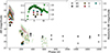 |
Fig. 1. Photometry of AT 2019azh. The IR photometry is shown with solid coloured symbols, while the extensive UVO photometry is shown using partially transparent symbols. Upper limits are indicated with downward facing triangles. The x-axis is broken as the omitted time period only contains upper limits. The inset plot shows the optical and IR light curves around peak in more detail. |
In Faris et al. (2024), the authors find that the redder TDE emission peaks later compared to bluer bands, as has been found in other TDEs (see e.g. Holoien et al. 2020). We fitted a second order polynomial to our H and K band photometry and determined the implied peak times to be 11.4 d and 14.8 d for H and K, respectively, continuing this trend. We note however, that we only have sparse data, so there is a large uncertainty on these peak times. The J-band data only declines, so our peak estimate is an upper limit of 17 d.
3.2. SED fitting with dust emission
To measure the temperature of the dust that is a possible source of the IR emission, we performed fits to the UVO+IR SED of AT 2019azh at the epochs where we have IR data. For each NIR epoch, we linearly interpolated between the closest two epochs for each UVO filter to generate the full SED, estimating the uncertainties at the interpolated epochs by adding the uncertainties of the closest two epochs in quadrature. We excluded UVO filters which do not have two observations within five days of the IR epoch. For the NEOWISE data, we did not interpolate between the first two epochs, as there is a large change in brightness (1.7 mag) and a six month gap between these observations, but we interpolated between the second and third epoch, as there is very little change in brightness (0.1 mag). The second NEOWISE epoch is very fortunately timed within 2 d of a NIR observation, and we assumed no evolution between these NEOWISE and NIR epochs.
We simultaneously fitted a linear combination of a ‘hot’ blackbody which we assume describes the contribution from the direct TDE emission, and a ‘cool’ blackbody which describes the contribution of the emission arising from the heated dust to the observed SED. For the ‘cool’ blackbody, we used a modified blackbody of the form B′ν(Tdust) = κabs, νBν(Tdust), where κabs, ν is the mass absorption coefficient for the dust at frequency ν, which is dependent on the choice of distribution of grain radii a, and the grain composition. We considered both single size distributions and multiple size distributions, where the number density of grains per grain radius is proportional to a−3.5 (the MRN grain size distribution; Mathis et al. 1977) from minimum size a = 0.005 μm up to a selected maximum size. For the modified blackbody, the observed flux density can be expressed as Fν, dust = (κabs, νMdBν(Tdust))/D2 where Md is the total dust mass and D is the luminosity distance to the TDE.
The temperature of the cool blackbody should be less than the dust sublimation temperature, Tsub, which is dependent on the grain size, composition and number density. Graphite grains able to survive temperatures 300 − 500 K larger than those of silicate, and larger grains have higher Tsub (Guhathakurta & Draine 1989; Baskin & Laor 2018). Dust survives at higher temperatures as the number density of grains, or equivalently the gas number density, increases, with graphite grains having Tsub = 1500 and 2000 K for gas number densities n ∼ 105 and 1011 cm−3, respectively (Baskin & Laor 2018). Making no assumption for the gas density, we conservatively limited the cool blackbody temperature to < 2200 K in our fits and initially made use of the κabs, ν for a single size distribution of 0.1 μm graphite dust, which has a high sublimation temperature. For the fitting, we employed the EMCEE python implementation of the Markov chain Monte Carlo (MCMC) method (Foreman-Mackey et al. 2013) to fit the points and derive uncertainties. We excluded some measurements from the fits, these are indicated in the figures. This is because the ori bands at 17 d and 38 d have a significant excess compared to the hot blackbody implied by the UV data. The origin of the excess could be strong Hα emission, as is indeed clear in the host and continuum subtracted spectra presented in Faris et al. (2024). Alternatively, there could be an intrinsic deviation from a thermal spectrum, as we discuss below.
We show the results of these fits in Fig. 2. In all epochs, there is an IR excess compared to the hot blackbody, so the IR emission does not simply represent the Rayleigh-Jeans tail of the TDE blackbody emission. Before 40 d, we can fit the SEDs for the epochs with only JHK observations using a cool blackbody with 0.1 μm graphite dust. The dust temperatures are very high, but potentially consistent with dust sublimation if the gas density was sufficiently high, approximately n ∼ 1011 to 1012 cm−3 (Baskin & Laor 2018). However, the best fit dust temperature in the second epoch at 7 d, where the SED extends to 4.6 μm, is ∼1000 K, much cooler than the surrounding epochs. If we exclude the measurements at 3.4 and 4.6 μm and only fit the interpolated JHK data with a hot dust component that is consistent with the surrounding epochs, we find a large deficit in flux density at 3.4 μm and 4.6 μm (see Fig. 3).
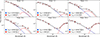 |
Fig. 2. SED fitting with two blackbodies (hotter TDE and cooler dust) for the observed UVO+IR SEDs at six epochs (labelled). Fitting was performed with a modified blackbody for the dust. The dust here is entirely composed of graphite with a grain size of 0.1 μm. Empty points are excluded from the fit. |
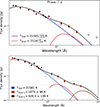 |
Fig. 3. Top: SED fitting with two blackbodies (hot TDE and cooler dust) for the observed UVO+IR SED at 7 d. Fitting was performed with a modified blackbody for the dust. The 3.4 μm and 4.6 μm data (open circles) are excluded from the fit, so that a fit with a high dust temperature is preferred. Bottom: SED fitting with three blackbodies (hot TDE and two dust components) at the same epoch, with a modified blackbody corresponding to graphite dust for both dust components. The TDE temperature is fixed. |
To investigate if any other dust grain size distribution can produce a good fit, we fitted the second epoch with a range of κabs, ν corresponding to graphite dust with different grain sizes, including both single and multiple size distributions. We used only graphite grains because the results of our fitting of the other epochs imply that high temperature dust is required. These fits are shown in Fig. C.3, with the reduced χ2 statistic listed. No composition yields a good fit. Although we can obtain good fits for hot 0.1 μm graphite dust in epochs −3 d, 17 d, and 38 d, the additional MIR data available at the second epoch is inconsistent with dust of this temperature and composition.
One possibility to fit the MIR data is to include an additional dust component with a lower temperature. We show such a fit in Fig. 3, where both dust components are composed of graphite with a single size of 0.1 μm. In this fit, the TDE component was subtracted from the overall SED and the two dust components were fitted to the remaining flux. The cooler dust has a rather low temperature of ∼630 K. Notably, the best fit temperature for the hotter dust is still consistent with the best fit temperatures found for the surrounding epochs that lack MIR data. This fit could imply that the NIR part of the SED is explained by hot dust at the sublimation radius of the TDE, while the MIR part would arise from much cooler dust much further out. We explore this scenario further in Sect. 3.4.
The SEDs in the final two epochs, where the phase is more than 200 d post-peak, have a much different shape, with a clear double peak. These can be fitted reasonably well with a modified blackbody, yielding cool dust temperatures of 600–700 K. Notably, this temperature is similar to that required for the cooler dust component inferred from the triple blackbody fit at +7 d. At these cooler temperatures, a graphite dust model is not necessarily required, and using different dust grain compositions can produce a range of temperatures and masses for the dust. This will be explored further in Sect. 3.4. In summary, the observed SEDs of AT 2019azh are consistent with a combination of direct TDE blackbody emission and cool dust at epochs later than 200 d, but for epochs earlier than 40 d, multiple dust components with different temperatures are required.
3.3. SED fitting with reprocessing models
An alternative explanation for the observed IR excess is direct emission from the TDE, which requires that the TDE spectrum deviates from a blackbody. This possibility has been discussed by a number of authors, who argue that the dominant absorption opacity at > 1 μm can be due to free-free processes and produce a power-law slope that is shallower than a blackbody (Lu & Bonnerot 2020; Roth et al. 2016, 2020)5. A detailed derivation of the expected continuum spectrum is given in Roth et al. (2020), who find that, under the assumptions of spherical symmetry and that the density drops as r−n with n > 1 near the surface of the emitting material, Lν ∝ ν(6 − 4n)/(2 − 3n). This connects the SED shape in the IR with the density of the material from the disrupted star.
We fitted our IR data at the four epochs before 40 d with a power-law function Lν ∝ να. The measured parameters are listed in Table 1, and the fits are shown in Fig. C.4. For a blackbody at the observed TDE temperatures we expect the emission to follow the Rayleigh–Jeans law, Lν ∝ ν2 at low frequencies. We observe shallower slopes at all epochs, which is visible as an IR excess in Fig. 2. The JHK SED is well fitted by a power law at −3 and 38 d, and fitted less well at 7 d and 17 d. We note that the JHK data in the 7 d fit is derived from interpolation, so this is not an independent measurement. The measured power-law index α decreases steadily and linearly over the 40 d period of our observations, becoming shallower at a rate of −0.015 per day. The corresponding values of power-law index for the density profile are initially very large, implying an extremely steep density profile. The power law at 7 d does not fit both the NIR and MIR part of the IR SED, with the MIR data having a different slope. This could be due to the interpolation used to estimate the NIR photometry at this epoch, evidence of excess IR emission due to dust at this epoch, or an indication that a single power-law slope does not hold for our data.
Results from fitting a power law Lν ∝ να to the IR SEDs observed for AT 2019azh.
3.3.1. The viewing-angle-dependent reprocessing model
To further explore the non-blackbody SED of AT 2019azh, we made use of the reprocessing framework presented in Thomsen et al. (2022) and Dai et al. (2018). This model utilises the radiative transfer code SEDONA and the general relativistic radiation magneto-hydrodynamics (GRRMHD) code HARMRAD to calculate the continuum emission from a super-Eddington accretion flow. Following the methods outlined in Thomsen et al. (2022), we obtained a 1D density, temperature, and velocity profile for a given inclination angle of the 3D accretion flow structure. This 1D structure was then converted to a spherical structure in SEDONA. The gas composition includes H, He, C, N, O, Na, Mg, Si, S, Ca, Ti, and Fe, with solar metallicity.
We initialised the radiative transfer simulation by launching millions of photon packages drawn from a blackbody spectrum, characterised by a temperature T0 = 106 K and luminosity Linj. These photon packages propagate through the 3D spherical geometry and undergo scattering, and absorption and re-emission events, transforming the initial blackbody to a reprocessed spectrum. SEDONA incorporates and models various emission and absorption processes including Compton scattering, free-free, bound-free, and bound-bound transitions (Kasen et al. 2006; Roth et al. 2016). Due to the significant energy contained in the radiation, all calculations are considered under non-local thermal conditions when calculating the ionisation and excitation. SEDONA was run iteratively at least 20 times to ensure the temperature has converged.
We produced a grid of models with viewing angles θ ∈ [50° ,60° ,70° ]; luminosities Linj ∈ [2, 4, 8, 16] L45, where L45 = 1045 erg s−1 and accretion rates Ṁacc ∈ [7,12,24] ṀEdd. As we lack GRRMHD models with higher values of Ṁacc than 24, we multiplicatively scaled the density profile of the Ṁacc = 24 ṀEdd case to approximate higher mass accretion rates, and produced models with density scaling parameters ρscale ∈ [1, 1.5, 2]. The grid is incomplete for 70°, where the extremely high densities for ρ ∈ [1.5, 2] caused the simulations to fail in most cases. In the GRRMHD simulations used to create the super-Eddington disc, the SMBH has MBH = 106 M⊙ and spin parameter a = 0.8. We found that models with Ṁacc ∈ [7,12] were not luminous enough to fit the data. This is consistent with the physically expected mass accretion rates – we discuss this below.
Figure 4 shows all the models with Ṁacc = 24 produced in our grid, alongside the observed data of AT 2019azh. The models reproduce the trends discussed in Thomsen et al. (2022). For a fixed value of Linj, the spectra emit more in the UVO as the density of the reprocessing envelope along the line of sight increases, which occurs either through higher accretion rates (i.e. increasing ρscale), or increasing the observed viewing angle. The 50° inclination angle is not able to reproduce the observed luminosity of AT 2019azh at any epoch. For smaller inclination angles, the spectrum becomes more X-ray dominated, so we would expect even lower luminosities in the UVO+IR region. We therefore rule out viewing angles of 50° or less. For 60° and 70°, the models are able to reproduce the observed luminosity in the UVO region.
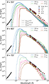 |
Fig. 4. Observed SEDs of AT 2019azh at epochs before 40 d, compared to the grid of simulated escaping spectra. The models have a wavelength grid such that the wavelength changes by 2% at each step, and are smoothed with a median filter of size 3. The top, middle, and bottom panels show models with 50°, 60°, and 70° inclinations, respectively. The colouring denotes the value of Linj as described in the legend, while the solid, dashed, and dotted lines represent models with a density profile scaling factor of 2, 1.5 and 1, respectively. We additionally show the X-ray spectrum observed at 20 d (Guolo et al. 2024) with black circles. |
In Fig. 5 we zoom in on the UVO+IR part of the spectrum for the 60° and 70° models. The NIR slope for AT 2019azh is shallower than the Rayleigh-Jeans part of a blackbody spectrum, and to reproduce this, we require a strong contribution from free-free emission. The strength of the free-free opacity is closely tied to the ionisation state, which decreases with increasing density (i.e. ρscale or θ), and increases with Linj. We discuss this in detail in Appendix A, and show the contribution of the free-free opacity and emission in Fig. A.1. In summary, for a significant contribution from free-free emission, the density and injected luminosity must be such that the ionisation level is high enough for bound-free processes not to dominate, but not so high that electron scattering dominates. In these latter two cases, the spectrum becomes more blackbody-like.
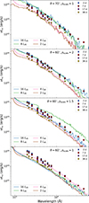 |
Fig. 5. As in Fig. 4 but zoomed into the UVO+IR region. The top panel shows the 70° inclination, whereas the other three panels have an inclination of 60°. The density profile scaling is indicated on the panels. |
For an inclination angle of 70°, the UVO data around peak is fitted reasonably well with Linj = 16 or 8 L45, although the model spectrum is slightly too luminous. For the 38 d epoch, the UVO part of the spectrum is well reproduced with Linj = 2 or 4 L45. In both cases, the IR data are too faint, with the MIR emission not well fitted at peak, and the NIR data not well fitted at 38 d. This is because the ionisation level is not high enough to produce the free-free emission required to reproduce the IR spectrum. In contrast, the 60° model with ρscale = 2 and Linj = 16 L45 is able to fit the entire spectrum at 7 d including all the IR data.
In Fig. 4 we also show the observed X-ray spectrum of AT 2019azh at 20 d, reported in Guolo et al. (2024). All of our models are much fainter than the observed X-rays. This could be explained by the assumption of spherical symmetry inherent in our 1D models, which prevents us from capturing 2D/3D effects such as photons scattering from different viewing angles to the line of sight (see Parkinson et al. 2025). We discuss this further in Sect. 4.1.
3.3.2. Inferring physical parameters from spectral modelling
From the best fitting model at peak, we measured the accretion rate at 7 d, and use analytical expectations for the evolution of the fallback rate to select models that should fit our data at the other epochs. The fallback timescale for the most tightly bound disrupted material for the tidal disruption of a star with mass m★ and radius r★ is given by (Evans & Kochanek 1989; Guillochon & Ramirez-Ruiz 2013; Rossi et al. 2021):
 (1)
(1)
and assuming that the fallback rate peaks at tfb, the post-peak time associated with a fallback mass accretion rate Ṁfb is calculated with
 (2)
(2)
Some quantity of the material that falls back will be lost to outflows in the form of a disc wind, so Ṁfb = Ṁacc+Ṁw. The wind value for Ṁacc = 24 ṀEdd measured in the hydrodynamical simulations from Thomsen et al. (2022) was Ṁw = 14 ṀEdd, implying Ṁfb = 38 ṀEdd for the total fallback rate. To estimate Ṁfb for our models with ρscale > 1, we assume that Ṁacc and Ṁw scale linearly with ρscale, so that Ṁfb = [57, 76] ṀEdd for ρscale = 1.5, 2. The results from Thomsen et al. (2022) show an increase of the ratio Ṁw/Ṁacc with increasing Ṁacc, so our approximation for Ṁfb is a lower limit.
Our best fitting models at −3 d and 7 d have ρscale = 2, which implies that Ṁfb(tfb) = 76 ṀEdd. We adopt the SMBH mass of MBH = 106.4 M⊙ derived from the velocity dispersement measurements of Wevers (2020) and Yao et al. (2023), and assume a simple stellar mass-radius relation of R★/R⊙ = (M★/M⊙)0.8. We also assume that the fallback rate peak coincided with the −3 d epoch. Equation (2) then implies a mass for the disrupted star of M★ ∼ 2.8 M⊙. With this value for M★, we derive expected fallback rates at 17 d and 38 d of Ṁfb(tfb+17) = 55 ṀEdd, Ṁfb(tfb+38) = 40 ṀEdd. These values are rather close to the expected Ṁfb values of 57 and 38 ṀEdd for ρscale = 1.5 and 1 respectively, so we expect these models to fit these epochs well.
As we assume that the injected luminosity arises from accretion, the values for Linj and Ṁacc are not independent. We make the simple approximation that Linj scales linearly with Macc to select models that we expect to reproduce the spectra at 17 d and 38 d. These models are shown in Fig. 6, and fitted the evolution of the TDE SED quite well. The optical and IR data in particularly are well fitted, but the UV data are somewhat more luminous than the models. Note that the model with ρscale = 1.5 and Linj = 12 L45 was not part of our initial grid.
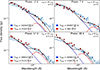 |
Fig. 6. Observed SEDs of AT 2019azh, compared with both the best fitting dust models as in Fig. 2, and selected reprocessing models. The SED at 7 d is well fitted by the model with ρscale = 2 and Linj = 16 L45. The models at 17 and 38 d assume that the density and luminosity scale linearly during the decline of the accretion rate. The reduced χ2 values associated with these models are listed in Table 2. |
The total luminosity available for injection is limited by the accretion rate, with Linj ≤ Lmax = ϵ Ṁaccc2 for some efficiency ϵ. For Ṁacc = 24,36,48 ṀEdd, corresponding to assumed accretion rates for our values of ρscale, and with the estimated SMBH mass of MBH = 106.4 M⊙ then Lmax = 24, 36, 48 LEdd ∼ 8, 11, 15 L45. Our best-fitting model at peak has Linj = 16 L45, broadly consistent but slightly larger than Lmax. Reducing the value of Linj to be consistent with this limit would not strongly effect the resulting spectral model.
To explain the mass accretion rates with a lower mass star, we would require a lower mass SMBH. For a solar mass star, the SMBH mass required for the best fit peak Ṁfb is MBH ∼ 106.16 M⊙, which is well within the uncertainties on our SMBH mass measurements. As Lmax ∝ MBH, so Lmax would also be halved for this smaller SMBH compared to our adopted value and so we would need to half the values of Linj to maintain physical consistency. The corresponding models are not luminous enough to fit the spectrum well, particularly in the IR. However, a somewhat lower value for MBH and corresponding lower value of M★ cannot be ruled out.
The luminosity we observed, i.e. the escaping luminosity Lesc, is less than the injected luminosity, as energy is lost to work done driving outflowing TDE material. Typical values of Lesc, measured directly from the model spectrum, are ∼0.1 − 0.2 × Linj, depending on the specific model. For example, the best-fitting model at 7 d with ρscale = 2, Linj = 16 L45, and θ = 60°, has Lesc/Linj = 0.2. There is a trend for this ratio to be larger for larger values of Linj. The difference between Lesc and the luminosity of the blackbody fit to the UVO data (measured in Sect. 3.2), LBB, represents the ‘missing energy’ that we do not directly observe from the TDE. The best fitting model at 7 d has LBB/Lesc = 0.05, i.e. the missing energy is 95% of the luminosity of the TDE at this epoch.
In order to directly compare whether the dust or reprocessing model best describes the data, we measured reduced χ-squared values for the best fitting dust models and the selected reprocessing models that we show in Fig. 6. The results are shown in Table 2. The quality of fits is comparable between the two models for the first two epochs, although the hot dust model at 7 d is a worse fit. The third and fourth epochs are less well fitted by the dust model if all the data, including the ori bands, is included. We note that the reprocessing models come from a sparse grid, so we would expect to find better χ-squared values if are grid was more densely sampled.
Selected models for the SEDs of AT 2019azh with IR data.
In summary, these reprocessing models can reproduce the entire UVO+IR SED of AT 2019azh, requiring a viewing angle of 60°; highly super-Eddington accretion, Ṁacc > 24 ṀEdd; and a high mass star, with M★ > 2. The time evolution can be well reproduced under a set of simple assumptions for the fallback accretion rates. We discuss the implications of these results and their consistency with other observations of this TDE in Sect. 4.1.
3.4. IR echo modelling
The most common explanation for an IR excess observed in TDEs is an IR echo from circumnuclear dust, and many IR echoes associated with optical TDEs have been observed (see e.g. van Velzen et al. 2016; Jiang et al. 2016, 2021b; Dou et al. 2016). As shown in Sects. 3.2 and 3.3, the IR brightness before 40 d is not consistent with single-temperature dust, but instead requires either a hotter and cooler dust component, or non-thermal TDE emission. We detect an IR excess at epochs later than 200 d which is consistent with cool dust emission, and we can model this as an IR echo. At late times, we no longer expect a non-thermal TDE spectrum due to free-free emission, as the accretion rates and thus densities are much lower. We therefore assumed that the TDE’s UVO SED is well modelled with a blackbody and subtracted the flux density associated with this blackbody at each epoch from the IR data to obtain the flux density associated only with the IR echo. The blackbody parameters were taken from the results of our blackbody fitting in Sect. 3.2, and the resulting IR echo light curve evolution is shown in Fig. 7. We also show the cooler dust component from the SED at 7 d, (shown in Fig. 3) after subtraction of both the TDE and hotter dust component. The observed J-band flux density after 200 d is consistent with the UVO blackbody, and is not shown. We omitted the NIR detections before 40 d, which arise from either much hotter dust, or non-thermal TDE emission. We did not propagate the uncertainties on the BB fitting.
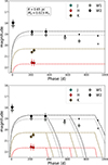 |
Fig. 7. Top: IR echo model for a spherical shell of silicate dust. The dust shell has a radius of 0.65 pc, to match the observed photometry between 200 and 400 d. The contribution of the hot TDE blackbody, and any hot dust emission at early times, has been subtracted from the data. The shell does not reproduce the observed drop in the MIR light curves, and under-predicts the potential cool dust component at early times. Bottom: IR echo models for different silicate dust clumps. The dust is at 0.65 pc from the TDE and has θ0 = 30°, 40°, 50°; θclump = 60°, 80°, 100°. The models with larger values of θclump decline at later times. |
3.4.1. Thin shell
We first attempted to model the IR echo with a spatially thin spherical shell of dust with radius R. We followed Maeda et al. (2015), and summarise here the key points. The dust shell has a temperature T(θ), with θ the angle between the observer line-of-sight and the vector directed from the centre of the shell to the observed shell volume element, and mass Md. Then the luminosity of the IR echo is:
 (3)
(3)
where κabs, ν is the mass absorption coefficient of the dust at frequency ν, which is determined by the dust properties. We assume a uniform number density for the shell. We can derive a time-dependent luminosity by relating t′, the time at which light emitted from a given volume element at θ is observed, to t, the time since the first light from the TDE, as follows:
 (4)
(4)
 (5)
(5)
We additionally assume that the temperature of the dust is determined by radiative equilibrium with the TDE flux:
 (6)
(6)
which determines the dust temperature T(t) for a given TDE luminosity evolution and dust shell radius. As discussed in van Velzen et al. (2016) and Lu et al. (2016), and shown in the examples from Maeda et al. (2015), such a model produces a square wave if the light travel time to the dust is larger than the characteristic timescale of the TDE.
We assumed that the pseudo-bolometric LC derived in Faris et al. (2024) is a good approximation for the total luminosity of the TDE at the wavelengths responsible for heating the dust, and used this as an input to the model. The free parameters are then the dust composition, which determines the mass absorption coefficient, and the mass and radius of the dust shell. The dust shell is spatially thin – this is an approximation for a more physical distribution of dust, that can be extended to larger radii. This is a reasonable approximation as the IR echo signal will be dominated by the emission arising at the inner part of the distribution, where the dust is hottest, the density highest and the IR echo has a shorter duration, due to shorter light travel times.
Our SED fitting in Sect. 3.2 implies that the dust temperatures are low (< 1000 K), much less than the sublimation temperature. We cannot then assume that the dust composition and radius is controlled by dust sublimation as a result of the TDE. Using a graphite dust composition, we require dust at ∼1 pc to reproduce the observed colours; however, silicate dust can be located more nearby, with a good fit to the observed colours at ∼0.65 pc (∼2 light years), shown in Fig. 7. Such a large radius for the dust shell creates a long-lived IR echo (twice the light travel time, i.e. ∼4 years), that does not reproduce the observed decline and drop in the MIR observations. Therefore, the spherical shell IR echo model cannot self-consistently reproduce both the timescale and the colours of the IR echo we observe. Additionally, the observed cool dust emission at 7 d is much more luminous than predicted by this model, implying that an additional dust component is required to fit these data.
3.4.2. Dust clumps
The temperature of the dust, and therefore the colour of the IR emission, is determined by the distance to the dust from the TDE. By altering the geometry of the dust, we can change the time evolution of the IR echo while still obtaining similar colours for the IR emission. We consider a dust clump, which we here simply approximate with a section of the overall spatially thin spherical shell with the same properties as in Sect. 3.4.1, at distance rclump. The section is defined by θclump, the angle between the observer line of sight and the centre of the section, and θ0 which is the opening angle of the section in both the polar and the azimuthal direction. The section has an infinitely-small radial thickness dr, the solid angle of the section is:
![Mathematical equation: $$ \begin{aligned} \begin{split} \Omega _{\mathrm{clump}} =&\int r_{\mathrm{clump}}^{2}\mathrm{sin}\theta \ \mathrm{d}\theta \mathrm{d}\phi \\ =&r_{\mathrm{clump}}^{2} \int _{\theta _{\mathrm{clump}}-\theta _{\mathrm{0}}/2}^{\theta _{\mathrm{clump}}+\theta _{\mathrm{0}}/2}\mathrm{sin}\theta \ \mathrm{d}\theta \int _{-\theta _{\mathrm{0}}/2}^{+\theta _{\mathrm{0}}/2}\mathrm{d}\phi \\ =&\theta _{\mathrm{0}} r_{\mathrm{clump}}^{2} [\mathrm{cos}(\theta _{\mathrm{clump}}-\theta _{0}/2) - \mathrm{cos}(\theta _{\mathrm{clump}}+\theta _{0}/2)], \end{split} \end{aligned} $$](/articles/aa/full_html/2026/04/aa56056-25/aa56056-25-eq21.gif) (7)
(7)
and the density of the clump is:
 (8)
(8)
The luminosity of the IR echo from this clump is:
![Mathematical equation: $$ \begin{aligned} \begin{split} L_{\mathrm{echo},\nu }(t)&= \int 4 \pi \kappa _{\mathrm{abs},\nu } B_{\nu } (T(\theta )) \rho _{\mathrm{clump}} \Omega _{\mathrm{clump}}\, \mathrm{d}r \\&= \frac{4 \pi c \kappa _{\mathrm{abs},\nu } M_d}{r_{\rm clump} [\mathrm{cos}(\theta _{\mathrm{clump}}-\theta _{0}/2) - \mathrm{cos}(\theta _{\mathrm{clump}}+\theta _{0}/2)]} \\&\quad \times \int _{\mathrm{max}([t-\frac{r_{\mathrm{clump}}}{c}(1-\mathrm{cos}(\theta _{\mathrm{clump}}+\theta _{0}/2))],0)}^{\mathrm{max}([t-\frac{r_{\mathrm{clump}}}{c}(1-\mathrm{cos}(\theta _{\mathrm{clump}}-\theta _{0}/2))],0)} B_{\nu }(T(t\prime )\mathrm{d}t\prime \end{split} \end{aligned} $$](/articles/aa/full_html/2026/04/aa56056-25/aa56056-25-eq23.gif) (9)
(9)
where t′ is defined as in Eq. (4) and the temperature evolution by Eq. (6)6.
To fit the IR LC after 200 d, we explored silicate dust clumps placed at approximately 0.65 pc, in order to match the observed colours of the IR echo. In Fig. 7 we show models arising from some dust clumps with rclump = 0.65 pc, θ0 = 30, 40, 50°, and θclump = 60, 80, 100°, respectively. These dust configurations produce IR echoes that rise as early as possible, to demonstrate that we expect only a small contribution from this dust at early times. The epoch at which the echo sharply declines is later for larger opening angles θclump. The slow decline after ∼400 d is not well reproduced by a spatially thin dust shell, but would be naturally produced by extending our model to include an extended distribution for the dust (see e.g. Nagao et al. 2017). Thus a dust clump with θ0 = 30° and θclump = 60°, with an extended dust distribution, could likely fit these data. However, given the lack of constraints on the many free parameters of the model, we choose not to further increase the model complexity. Using Eq. (9), we can calculate the dust covering factor directly by measuring the total radiated energy of the IR echo (Edust) and comparing to the observed total radiated energy of the TDE (ETDE). For the model with θ0 = 40° and θclump = 80°, we find a covering factor Edust/ETDE ∼ 1%. The mass of dust in this model is 0.01 M⊙.
In order to produce the more luminous emission associated with the cool dust at 7 d, an additional dust clump is required. We measured the temperature of this dust to be very similar to that of the dust at late times, implying it lies at a similar distance. As the rise of the echo from this dust is very fast, θclump must be small, corresponding to a clump close to the line of sight. Furthermore, the opening angle θ0 must also be small, to prevent this dust dominating the IR echo signal after 200 d. The LC resulting from a configuration with θ0 = 5° and θclump = 10° is shown in Fig. B.2, and can reproduce the 7 d epoch and then decline fast enough to not contribute significantly at later epochs.
Given that the possible cool dust emission at early times could be explained by a distant dust clump close to the line of sight, we now return to the possibility of hot dust as an explanation for the early NIR emission. Such dust must be close to the sublimation radius for the given graphite dust composition, in order to produce the very high temperatures found in Sect. 3.2. Then, for similar reasons as for the cool dust above, the dust must be confined to a clump that is close to the line of sight and has a small opening angle. The most extreme example, a clump almost in the line of sight with a very small opening angle, will produce a echo light curve that follows the TDE luminosity evolution and decline as fast as possible, as there are no light travel time effects. In this case, the IR echo evolution is driven purely by the evolution of the dust temperature. As shown in Fig. B.2, we find that dust with a sufficient mass to fit the first epoch well over-predicts the NIR brightness at 200 d. Additionally, such dust does not produce the rise observed in the NIR bands at early times, instead declining rapidly. This NIR LC shape can be produced by increasing the dust opening angle, but this increases the HK luminosity at 200 d. It is therefore difficult to explain the early time NIR data with at clump of hot dust. For further discussion, see Appendix B.
Interestingly, there is an additional NEOWISE detection in the W1 band at 1640 d, shown in Fig. 1. The W1 mag is fainter than at 212 and 363 d, and there is no W2 detection. For a time lag of 1640 d, the minimum radial distance to the dust, occurring in the case that the dust is on the far side of the SMBH, is 1640/2 light days, i.e. 0.69 pc. The detection is thus consistent with the presence of an additional dust clump further out than the first, and given that the epochs immediately before and after the detection yield no detection, it should have a relatively small opening angle.
In summary, it is possible to explain the observed IR data of AT 2019azh after 200 d with an IR echo arising from a clump of silicate dust that lies ∼0.65 pc from the TDE. There is additionally evidence of further dust clumps at similar distances from the SMBH but different angles. It is important to note that these parameters are not strongly constrained. For example, using different dust compositions will change the distance to the dust (larger radius for larger proportions of graphite) and our sparse photometry does not properly constrain the rise and fall of the echo.
4. Discussion
4.1. Reprocessing models for AT 2019azh
Infrared detections of TDEs have previously been interpreted as arising from an IR echo from dust. However, in the case of AT 2019azh, the IR emission at epochs before 40 d is difficult to explain as dust emission. This is primarily because we are unable to reproduce the SED that extends to 4.6 μm at 7 d with a single blackbody corresponding to any graphite dust composition. It is possible to fit the NIR SED at the other early epochs with very hot graphite dust, but a consistent temperature cannot simultaneously fit the entire SED we observe at 7 d, drastically underestimating the 3.4 μm and 4.6 μm flux. It is possible to introduce multiple dust components to better fit the SED, requiring a dust component at the sublimation radius to produce the hot emission seen in the NIR, and a substantially further out dust component to produce the bright, but much cooler MIR emission. We show above that a dust clump close to the line of sight can explain the cool emission, but any dust clump at the sublimation radius that can reproduce the early emission will not fade sufficiently fast to fit our NIR observations at 200 d. We therefore disfavour the hot dust interpretation for the early NIR emission. However, it is difficult to rule out this scenario entirely, due to the limited data available.
The alternative explanation is that the IR emission arises primarily directly from the TDE. To produce an IR excess compared to a hot blackbody describing the TDE emission, the free-free opacity should dominate in the IR, which requires a geometrically and optically thick reprocessing envelope. The predicted spectrum follows a power law, and our NIR data can be well fitted with such a power law. However, as we only have three NIR bands, this power-law fit is not well-constrained. We found that the evolution of the required power-law index implies a very steep density distribution outside the emitting region at peak that rapidly and linearly becomes shallower. A major powering mechanism invoked to produce the UVO emission from TDEs is stream-stream collisions. Lu & Bonnerot (2020) presents the collision-induced outflow (CIO) model for TDEs, in which self-intersection of the fallback stream unbinds a large amount of shocked gas and produces an outflow. They predict that the reprocessing in the unbound envelope will produce a shallow slope in the IR, Lν ∝ ν∼0.5, rather close to our observed values at ∼39 d.
The viewing angle dependent model of Dai et al. (2018) and Thomsen et al. (2022) can well reproduce the IR SED of AT 2019azh, while simultaneously fitting the UVO data. The best fit parameters require a relatively steep viewing angle for the observer of ∼60° and very high accretion rates of Macc > 24 ṀEdd at peak. We also found that to reproduce the large value of Mfb that is implied by our spectral fitting at peak, we require a high mass star to be disrupted, with M★ > 2 M⊙ being the preferred mass. The starburst age for the host galaxy of AT 2019azh has been measured as 200 ± 30 Myr (Wevers & French 2024), and a 3 M⊙ star has a main sequence lifetime of ∼300 Myr (Kippenhahn et al. 2013); therefore there is a population of such stars available to be disrupted. Light curve fitting codes have been used to estimate M★ for AT 2019azh: the widely used code MOSFiT (Guillochon et al. 2018) has found very low values of 0.1 M⊙ (Hinkle et al. 2021a; Faris et al. 2024) as well as a high value of ∼4 M⊙ (Hammerstein et al. 2023). Neither result is secure, with Faris et al. (2024) arguing that the low mass values are not self-consistent, and the SMBH mass estimated in the results of Hammerstein et al. (2023) being an order of magnitude larger than that derived from the velocity dispersion measurements. The high luminosity of AT 2019azh compared to the TDE population is also naturally explained if the disrupted star has a larger mass compared to the general population, and therefore a larger fallback rate. We note that there are many assumptions that go into this measurement. Some examples include that: Eq. (2) is not expected to hold for early times when the original structure of the disrupted star still impacts the light curve evolution (Guillochon & Ramirez-Ruiz 2013); the relationship between the peak optical luminosity in any particular band and the peak accretion rate is not clear; and our sparse grid means we do not have a precise measurement of the accretion rate or the inclination angle.
As well as fitting the UVO+IR SED, the X-ray behaviour of AT 2019azh is also well described by the viewing angle dependent reprocessing model, with the viewing angle we obtain. The X-ray emission in this model is prompt, but the X-rays are reprocessed in the optically thick material. The optical depth through the observer line of sight depends on the viewing angle and on the mass accretion rate of material. At low viewing angles (close to the pole), X-rays efficiently escape at all times, and the X-ray luminosity is always large compared to the UVO luminosity. At high viewing angles, the opposite is the case. At intermediate angles, the mass accretion rate is important: X-rays are suppressed at early times while the accretion rates are high, but as the accretion rate drops the optical depth decreases and the ratio of the X-ray to UVO luminosity increases. X-ray observations of AT 2019azh show this behaviour, described in Guolo et al. (2024) as a late-time brightening. AT 2019azh is detected at early times (20 d) but the ratio of UVO to X-ray luminosity is of order 103. By 225 d, this ratio has become of order unity, and it remains so until 404 d. As previously mentioned, the 1-D nature of our modelling prevents direct comparison of the observed X-rays to our model spectra. However, the observed X-ray behaviour is consistent with the expectations for intermediate viewing angles, such as our predicted viewing angle of 60°. The CIO model also predicts that an X-ray brightening can occur in some TDEs, due to the CIO blocking the line of sight to the accretion disc at early times. Therefore, their scenario is also qualitatively consistent with the X-ray observations of AT 2019azh.
A single epoch of spectro-polarimetry of AT 2019azh was observed at 16 d and this data was presented and analysed in Leloudas et al. (2022). They found that the peak of emission lines observed was depolarised, while the wings showed polarisation peaks, indicative of electron scattering. Leloudas et al. (2022) argue that the polarimetric observations are consistent with the viewing angle dependent reprocessing model similar to that which we present, with super-Eddington accretion and a massive reprocessing envelope.
In Goodwin et al. (2022), analysis of the radio observations of AT 2019azh revealed an outflow occurring at early times (10 d pre-peak), around the time of the stellar disruption. They argue that the CIO model would produce an outflow with similar properties to that inferred from the radio data, and that the early timing can be explained by the outflow being launched through the stream-stream collision. An accretion driven outflow is disfavoured by the lack of X-rays at early times unless there is significant obscuration of the X-rays, as in the viewing angle dependent model.
In summary, the multi-wavelength observations of AT 2019azh seem consistent with either the viewing angle dependent model or the CIO model for TDE emission. We explored the viewing angle dependent model in greater depth, and show that we can reproduce the UVO+IR SED, and constrain the TDE viewing angle. We encourage further exploration of both models.
4.2. Dust properties
The IR emission from AT 2019azh later than 200 d is consistent with an IR echo from ∼0.01 M⊙ of dust confined to a relatively small region approximately 0.65 pc from the central SMBH. Assuming a typical gas to dust mass ratio of 100, this quantity of dust would correspond to ∼1 M⊙ of gas. The inner parsec around the central SMBH thus appears to be quite sparse, consistent with the nature of the host galaxy as quiescent. We additionally observe a short lived-late time IR flare that is consistent with another dust clump, at similar or greater distance than the first one. The observations are consistent with a distribution of clumpy clouds of gas and dust, similar to those observed in the Milky Way, where tens of gas clouds have been observed within 0.5–2 pc of the SMBH Sgr A*, although these clouds are much more massive (∼104 M⊙) (Mezger et al. 1996; Christopher et al. 2005).
Given that we have concluded that the early time IR excess is not due to dust, we never observe very hot dust in connection with AT 2019azh. This implies that the TDE itself does not sublimate a significant amount of dust, and therefore the dust distribution is independent of the TDE flare. The dust properties we infer are dependent on a number of simplifying assumptions about the TDE emission, which are not necessarily valid. First, the inferred luminosity of the TDE we use arises from blackbody fitting of the UVO observations. As discussed above, AT 2019azh was observed to produce significant X-ray emission and furthermore, it is expected that TDEs produce significant emission in the extreme-UV which we cannot directly observe. Integrating the SEDs of the models we present in Sect. 3.3.1, we find that the total luminosity of the best fitting models is ∼10 times that of the blackbody luminosity at the same epoch. This energy can be efficiently absorbed by the dust, and will require the dust to be more distant for our IR echo model to match the observed IR SED. If the dust is much more distant, then a smaller opening angle for the dust is required to produce the same timescale flare than for closer dust. The > 0.65 pc dust radius we infer here is larger than has been previously inferred for most TDE IR echoes in the literature (see e.g. van Velzen et al. 2016; Masterson et al. 2024), although a recent study found a large radius of > 1.2 pc for the dust echo arising from the TDE AT 2019qiz Wu et al. (2025).
Independent measurements of the density and location of the circumnuclear material around the SMBH hosting AT 2019azh arise from radio observations. Goodwin et al. (2022) found fluctuations in the synchrotron energy index observed for AT 2019azh, and argue that an inhomogenous circumnuclear medium could explain these observations and Burn et al. (2025) find an unusually flat density profile within the inner 0.1 pc surrounding the SMBH, implying a relatively dense environment. Additionally, Zhuang et al. (2025) argue that the multiple radio flares AT 2019azh exhibited significantly after the peak optical emission (∼350 and 600 d) were produced by the collision of the TDE outflow with multiple circumnuclear gas clouds, each producing a luminous radio flare. By modelling the flare associated with the scenario, they find that these clouds should lie at 0.1 pc and 0.2 pc, and have radii of 0.04 and 0.08 pc, respectively. These clouds are much closer than we infer for the dust cloud that produces the IR echo, and are close to the sublimation radius for AT 2019azh. We therefore expect to see high temperatures for any surviving dust in these clouds. As described above, such clouds with relatively large radii will be too luminous at > 200 d to reproduce the faint NIR emission observed. An alternative possibility is that all the dust within these clouds could be destroyed, if the intrinsic bolometric luminosity if the TDE is higher than that inferred from the blackbody luminosity. The sublimation radius increases approximately  , implying that if we are truly underestimating the peak luminosity by a factor of 10, the sublimation radius would be ∼0.28 pc for the graphite dust with a multiple size distribution, and any dust in the above clouds would be destroyed. If the sublimation radius is truly this large, then radio observations are essential in probing the smaller physical scales where the dust has been destroyed. Meanwhile, the IR observations complement the radio, by tracing the larger physical scales which will not be reached by the slower TDE outflows for many years.
4.3. Implications for the TDE population
There is a small sample of TDEs in the literature that have been observed close to the peak in the IR. All of these that we know of come from the NEOWISE survey, with no peak NIR observations previously reported. In the upper panel of Fig. 8 we compare the W1 photometry from AT 2019azh with the sample of NEOWISE observed TDEs presented in Jiang et al. (2021b). The peak luminosity of AT 2019azh is quite typical for this sample of objects and the light curve evolution strongly resembles the TDE AT 2018dyb (also known as ASASSN-18pg; Holoien et al. 2020; Leloudas et al. 2019), as well as being quite similar to ASASSN-14li and AT 2018hyz, with slight offsets in luminosity. There are only four TDEs in this sample that have MIR observations within 30 d of their peak; however, three of these exhibit a very similar MIR photometric evolution as AT 2019azh, with a sharp decline between the first observation and the later observations. It follows that, similarly to AT 2019azh, the peak MIR emission could be arising from direct TDE emission rather than emission from dust in these TDEs.
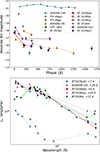 |
Fig. 8. Upper panel: NEOWISE W1 absolute magnitudes for AT 2019azh, alongside the sample of IR-detected TDEs presented in Jiang et al. (2021b). Lower panel: SEDs of TDEs in the literature with IR observations near to the TDEs optical peak. The MIR data are taken from Jiang et al. (2021b) and Swift data are taken from Hinkle et al. (2021b). Optical data for AT 2018hyz, AT 2018dyb, AT 2018zr, and ASASSN-14li are taken from Hung et al. (2020), Holoien et al. (2020), Holoien et al. (2019), and Holoien et al. (2016), respectively. The listed epoch is with respect to peak, except for ASASSN-14li, where it is with respect to the first detection. |
To further explore this, we show the SEDs of these TDEs at the epoch of the first MIR observation in the lower panel Fig. 8. The figure shows that the SED of AT 2018dyb is remarkably similar to that of AT 2019azh at an almost identical epoch, in both the UVO and MIR regions. In particular, the W1 − W2 colour is similar to that of AT 2019azh. This indicates that a reprocessing scenario could potentially explain the IR excess seen in this TDE. The other TDEs show variety, with both AT 2018hyz and AT 2018zr being less luminous in the UV, indicating a cooler and more thermal spectrum, or potentially host dust extinction, while ASASSN-14li appears both significantly less luminous and displays a U-shaped SED that is indicative of hot dust emission, as claimed in Jiang et al. (2016). Furthermore, the W1 − W2 colours of AT 2018zr and AT 2018hyz are also redder than those of the other TDEs. These TDEs are additionally all observed later than 20 d, in contrast with AT 2019azh and AT 2018dyb which are observed at ∼7 d, preventing a direct comparison. As we lack the NIR data to constrain the wavelength region between 1 and 2 μm, it is difficult to conclusively determine the origin of the IR emission in these cases.
Additionally to those TDEs observed at early times with NEOWISE, indications of reprocessing envelopes have been observed in other TDEs without such data. The TDE AT 2020mot exhibited a strong excess in i-band throughout its evolution, as well as a bump at 80 d post-peak, which Newsome et al. (2024) argued arose from multiple dust components within 0.1 pc of the TDE. Although the bump cannot be explained easily with the reprocessing model, it is possible that the persistent red excess was due to free-free emission. Newsome et al. (2024) argue that a ring of dust placed at ∼10−3 pc could explain the persistent excess, but this dust would be well within the expected sublimation radius. In Earl et al. (2025), the authors argue that the SED of the TDE AT 2020nov is best fit with the inclusion of a reprocessing envelope, with the z-band data in particular being poorly fitted with a simple blackbody model. NIR observations would have placed even stronger constraints on these two models.
5. Conclusions
In this work, we present IR observations of the TDE AT 2019azh and examine whether they are consistent with emission from dust heated by the TDE, or direct emission from the TDE in a reprocessing scenario. We summarise our findings as follows:
-
AT 2019azh exhibits a significant IR excess compared to a blackbody fit to the UVO data. The excess in the NIR alone before 40 d can be fitted by a blackbody corresponding to very hot (> 2000 K) graphite dust, but the NIR and MIR data together cannot be consistently fitted.
-
The IR excess exhibits a power-law shape, as predicted for non-thermal emission arising from free-free opacity in the IR in TDEs. This requires the presence of a dense reprocessing envelope.
-
The early time UVO+IR SED can be well-reproduced by spectral models produced from simulations of emission from a super-Eddington accretion flow. This model is viewing-angle dependent, and by comparing the SED to these models, we find that a viewing angle of ∼60° is necessary to reproduce the data. The implied mass accretion rate indicates that the disrupted star had a mass M★ > 2 M⊙.
-
The X-ray brightening of AT 2019azh supports a reprocessing scenario, with either the viewing-angle-dependent model or the CIO model qualitatively reproducing the observations.
-
Although the IR SED at early times can be fitted with hot dust associated with dust sublimation, such dust would be expected to still be hot and luminous at later epochs, and is thus disfavoured due to the faintness of the NIR data at epochs after 200 d. We favour the reprocessing scenario to explain the IR excess at early times.
-
Late time IR data show the presence of an IR echo from relatively cold (< 1000 K) dust. We model the IR echo and show that the dust must be distant from the TDE (> 0.65 pc) to have these low temperatures, and must have a relatively small geometrical covering factor in order to consistently produce an IR echo with a short timescale. We find evidence of a clumpy distribution of circumnuclear clouds, which is consistent with evidence of a similar distribution observed in the radio, although probing different distances from the SMBH.
-
Considering the small sample of previous TDEs observed close to the peak in the IR, we find that AT 2018dyb potentially also exhibited an IR excess due to non-thermal TDE emission.
Further observations of TDEs in the IR will be able to measure the relative rates of TDEs that show such a non-thermal IR excess, and determine whether these are consistent with the expected distribution of viewing angles for TDEs. Furthermore, multi-wavelength observations of TDEs that include the IR will be able to produce observables that can determine which reprocessing model is responsible for the TDEs we observe, and we invite further modelling efforts to capitalise on this. As in the case of AT 2019azh, observing both in the NIR and MIR will be crucial for distinguishing between non-thermal emission, and dust emission. Given that the NEOWISE survey has ended, future MIR facilities such as the NEO Surveyor (Mainzer et al. 2023) and SPHEREx (Alibay et al. 2023) will be essential.
Acknowledgments
T.M.R. thanks Thomas Wevers, Yanan Wang, Iair Arcavi and Peter Clark for helpful comments during preparation of the manuscript. We thank the anonymous referee for their constructive comments that improved the quality of the manuscript. T.M.R is part of the Cosmic Dawn Center (DAWN), which is funded by the Danish National Research Foundation under grant DNRF140. T.M.R and S. Mattila acknowledge support from the Research Council of Finland project 350458. T.N. and H.K. acknowledge support from the Research Council of Finland projects 324504, 328898, and 353019. S. Moran is funded by Leverhulme Trust grant RPG-2023-240. LT and LD acknowledge support from the National Natural Science Foundation of China and the Hong Kong Research Grants Council (N_HKU782/23, HKU17305124). CPG acknowledges financial support from the Secretary of Universities and Research (Government of Catalonia) and by the Horizon 2020 Research and Innovation Programme of the European Union under the Marie Skłodowska-Curie and the Beatriu de Pinós 2021 BP 00168 programme, from the Spanish Ministerio de Ciencia e Innovación (MCIN) and the Agencia Estatal de Investigación (AEI) 10.13039/501100011033 under the PID2023-151307NB-I00 SNNEXT project, from Centro Superior de Investigaciones Científicas (CSIC) under the PIE project 20215AT016 and the program Unidad de Excelencia María de Maeztu CEX2020-001058-M, and from the Departament de Recerca i Universitats de la Generalitat de Catalunya through the 2021-SGR-01270 grant.FEB acknowledges support from ANID-Chile BASAL CATA FB210003, FONDECYT Regular 1241005, and Millennium Science Initiative, AIM23-0001. This work is partially based on observations collected at the European Southern Observatory under ESO programme 199.D-0143(Q). This research was partly based on observations made with the Nordic Optical Telescope (program IDs: P59-506 and P68-505) owned in collaboration by the University of Turku and Aarhus University, and operated jointly by Aarhus University, the University of Turku and the University of Oslo, representing Denmark, Finland and Norway, the University of Iceland and Stockholm University at the Observatorio del Roque de los Muchachos, La Palma, Spain, of the Instituto de Astrofisica de Canarias. This publication makes use of data products from the Two Micron All Sky Survey, which is a joint project of the University of Massachusetts and the Infrared Processing and Analysis Center/California Institute of Technology, funded by the National Aeronautics and Space Administration and the National Science Foundation. This publication makes use of data products from the Near-Earth Object Wide-field Infrared Survey Explorer (NEOWISE), which is a joint project of the Jet Propulsion Laboratory/California Institute of Technology and the University of California, Los Angeles. NEOWISE is funded by the National Aeronautics and Space Administration. This work made use of Astropy: a community-developed core Python package and an ecosystem of tools and resources for astronomy (Astropy Collaboration Astropy Collaboration 2013, 2018, 2022).
References
- Alard, C., & Lupton, R. H. 1998, ApJ, 503, 325 [Google Scholar]
- Alibay, F., Sindiy, O. V., Jansma, P. A. T., et al. 2023, 2023 IEEE Aerospace Conference, 1 [Google Scholar]
- Almeida, A., Anderson, S. F., Argudo-Fernández, M., et al. 2023, ApJS, 267, 44 [NASA ADS] [CrossRef] [Google Scholar]
- Arcavi, I., Gal-Yam, A., Sullivan, M., et al. 2014, ApJ, 793, 38 [Google Scholar]
- Astropy Collaboration (Robitaille, T. P., et al.) 2013, A&A, 558, A33 [NASA ADS] [CrossRef] [EDP Sciences] [Google Scholar]
- Astropy Collaboration (Price-Whelan, A. M., et al.) 2018, AJ, 156, 123 [Google Scholar]
- Astropy Collaboration (Price-Whelan, A. M., et al.) 2022, ApJ, 935, 167 [NASA ADS] [CrossRef] [Google Scholar]
- Baskin, A., & Laor, A. 2018, MNRAS, 474, 1970 [Google Scholar]
- Bennett, C. L., Larson, D., Weiland, J. L., & Hinshaw, G. 2014, ApJ, 794, 135 [Google Scholar]
- Bonnerot, C., Lu, W., & Hopkins, P. F. 2021, MNRAS, 504, 4885 [NASA ADS] [CrossRef] [Google Scholar]
- Brennan, S. J., & Fraser, M. 2022, A&A, 667, A62 [NASA ADS] [CrossRef] [EDP Sciences] [Google Scholar]
- Burn, M., Goodwin, A. J., Anderson, G. E., et al. 2025, ApJ, 993, 207 [Google Scholar]
- Christopher, M. H., Scoville, N. Z., Stolovy, S. R., & Yun, M. S. 2005, ApJ, 622, 346 [Google Scholar]
- Dai, L., McKinney, J. C., Roth, N., Ramirez-Ruiz, E., & Miller, M. C. 2018, ApJ, 859, L20 [Google Scholar]
- Donley, J. L., Brandt, W. N., Eracleous, M., & Boller, T. 2002, AJ, 124, 1308 [NASA ADS] [CrossRef] [Google Scholar]
- Dou, L., Wang, T.-G., Jiang, N., et al. 2016, ApJ, 832, 188 [Google Scholar]
- Dwek, E. 1983, ApJ, 274, 175 [NASA ADS] [CrossRef] [Google Scholar]
- Earl, N., French, K. D., Ramirez-Ruiz, E., et al. 2025, ApJ, 983, 28 [Google Scholar]
- Evans, C. R., & Kochanek, C. S. 1989, ApJ, 346, L13 [Google Scholar]
- Faris, S., Arcavi, I., Makrygianni, L., et al. 2024, ApJ, 969, 104 [Google Scholar]
- Fitzpatrick, E. L. 1999, PASP, 111, 63 [Google Scholar]
- Foreman-Mackey, D., Hogg, D. W., Lang, D., & Goodman, J. 2013, PASP, 125, 306 [Google Scholar]
- French, K. D., Wevers, T., Law-Smith, J., Graur, O., & Zabludoff, A. I. 2020, Space Sci. Rev., 216, 32 [CrossRef] [Google Scholar]
- French, K. D., Earl, N., Novack, A. B., et al. 2023, ApJ, 950, 153 [NASA ADS] [CrossRef] [Google Scholar]
- Gezari, S. 2021, ARA&A, 59, 21 [NASA ADS] [CrossRef] [Google Scholar]
- Goodwin, A. J., van Velzen, S., Miller-Jones, J. C. A., et al. 2022, MNRAS, 511, 5328 [NASA ADS] [CrossRef] [Google Scholar]
- Graham, J. R., Meikle, W. P. S., Selby, M. J., et al. 1983, Nature, 304, 709 [NASA ADS] [CrossRef] [Google Scholar]
- Guhathakurta, P., & Draine, B. T. 1989, ApJ, 345, 230 [NASA ADS] [CrossRef] [Google Scholar]
- Guillochon, J., & Ramirez-Ruiz, E. 2013, ApJ, 767, 25 [NASA ADS] [CrossRef] [Google Scholar]
- Guillochon, J., Manukian, H., & Ramirez-Ruiz, E. 2014, ApJ, 783, 23 [NASA ADS] [CrossRef] [Google Scholar]
- Guillochon, J., Nicholl, M., Villar, V. A., et al. 2018, ApJS, 236, 6 [NASA ADS] [CrossRef] [Google Scholar]
- Guolo, M., Gezari, S., Yao, Y., et al. 2024, ApJ, 966, 160 [NASA ADS] [CrossRef] [Google Scholar]
- Hammerstein, E., van Velzen, S., Gezari, S., et al. 2023, ApJ, 942, 9 [NASA ADS] [CrossRef] [Google Scholar]
- Hinkle, J. T., Holoien, T. W. S., Auchettl, K., et al. 2021a, MNRAS, 500, 1673 [Google Scholar]
- Hinkle, J. T., Holoien, T. W. S., Shappee, B. J., & Auchettl, K. 2021b, ApJ, 910, 83 [NASA ADS] [CrossRef] [Google Scholar]
- Holoien, T. W. S., Kochanek, C. S., Prieto, J. L., et al. 2016, MNRAS, 455, 2918 [NASA ADS] [CrossRef] [Google Scholar]
- Holoien, T. W. S., Huber, M. E., Shappee, B. J., et al. 2019, ApJ, 880, 120 [NASA ADS] [CrossRef] [Google Scholar]
- Holoien, T. W. S., Auchettl, K., Tucker, M. A., et al. 2020, ApJ, 898, 161 [NASA ADS] [CrossRef] [Google Scholar]
- Hung, T., Foley, R. J., Ramirez-Ruiz, E., et al. 2020, ApJ, 903, 31 [NASA ADS] [CrossRef] [Google Scholar]
- Jiang, N., Dou, L., Wang, T., et al. 2016, ApJ, 828, L14 [Google Scholar]
- Jiang, N., Wang, T., Dou, L., et al. 2021a, ApJS, 252, 32 [Google Scholar]
- Jiang, N., Wang, T., Hu, X., et al. 2021b, ApJ, 911, 31 [NASA ADS] [CrossRef] [Google Scholar]
- Kasen, D., Thomas, R. C., & Nugent, P. 2006, ApJ, 651, 366 [NASA ADS] [CrossRef] [Google Scholar]
- Kippenhahn, R., Weigert, A., & Weiss, A. 2013, Stellar Structure and Evolution (Berlin, Heidelberg: Springer) [Google Scholar]
- Kool, E. C., Reynolds, T. M., Mattila, S., et al. 2020, MNRAS, 498, 2167 [NASA ADS] [CrossRef] [Google Scholar]
- Lang, D. 2014, AJ, 147, 108 [Google Scholar]
- Leloudas, G., Dai, L., Arcavi, I., et al. 2019, ApJ, 887, 218 [NASA ADS] [CrossRef] [Google Scholar]
- Leloudas, G., Bulla, M., Cikota, A., et al. 2022, Nat. Astron., 6, 1193 [NASA ADS] [CrossRef] [Google Scholar]
- Liu, X.-L., Dou, L.-M., Chen, J.-H., & Shen, R.-F. 2022, ApJ, 925, 67 [NASA ADS] [CrossRef] [Google Scholar]
- Loeb, A., & Ulmer, A. 1997, ApJ, 489, 573 [Google Scholar]
- Lu, W., & Bonnerot, C. 2020, MNRAS, 492, 686 [NASA ADS] [CrossRef] [Google Scholar]
- Lu, W., Kumar, P., & Evans, N. J. 2016, MNRAS, 458, 575 [Google Scholar]
- Maeda, K., Nozawa, T., Nagao, T., & Motohara, K. 2015, MNRAS, 452, 3281 [Google Scholar]
- Mainzer, A., Bauer, J., Cutri, R. M., et al. 2014, ApJ, 792, 30 [Google Scholar]
- Mainzer, A. K., Masiero, J. R., Abell, P. A., et al. 2023, Planet. Sci. J., 4, 224 [Google Scholar]
- Masterson, M., De, K., Panagiotou, C., et al. 2024, ApJ, 961, 211 [NASA ADS] [CrossRef] [Google Scholar]
- Masterson, M., De, K., Panagiotou, C., et al. 2025, ApJ, 988, L48 [Google Scholar]
- Mathis, J. S., Rumpl, W., & Nordsieck, K. H. 1977, ApJ, 217, 425 [Google Scholar]
- Mattila, S., Pérez-Torres, M., Efstathiou, A., et al. 2018, Science, 361, 482 [Google Scholar]
- Meisner, A. M., Lang, D., Schlafly, E. F., & Schlegel, D. J. 2021, Res. Notes Am. Astron. Soc., 5, 168 [Google Scholar]
- Meisner, A. M., Lang, D., & Schlegel, D. J. 2017, AJ, 153, 38 [Google Scholar]
- Meisner, A. M., Lang, D., & Schlegel, D. J. 2018, AJ, 156, 69 [NASA ADS] [CrossRef] [Google Scholar]
- Metzger, B. D. 2022, ApJ, 937, L12 [NASA ADS] [CrossRef] [Google Scholar]
- Mezger, P. G., Duschl, W. J., & Zylka, R. 1996, A&ARv, 7, 289 [NASA ADS] [CrossRef] [Google Scholar]
- Mummery, A., Guolo, M., Matthews, J., et al. 2025, MNRAS, 544, 2262 [Google Scholar]
- Nagao, T., Maeda, K., & Yamanaka, M. 2017, ApJ, 835, 143 [NASA ADS] [CrossRef] [Google Scholar]
- Newsome, M., Arcavi, I., Howell, D. A., et al. 2024, ApJ, 961, 239 [Google Scholar]
- Parkinson, E. J., Knigge, C., Dai, L., et al. 2025, MNRAS, 540, 3069 [Google Scholar]
- Phinney, E. S. 1989, in The Center of the Galaxy, ed. M. Morris, 136, 543 [Google Scholar]
- Piran, T., Svirski, G., Krolik, J., Cheng, R. M., & Shiokawa, H. 2015, ApJ, 806, 164 [Google Scholar]
- Rees, M. J. 1988, Nature, 333, 523 [Google Scholar]
- Reynolds, T. M., Mattila, S., Efstathiou, A., et al. 2022, A&A, 664, A158 [NASA ADS] [CrossRef] [EDP Sciences] [Google Scholar]
- Rossi, E. M., Stone, N. C., Law-Smith, J. A. P., et al. 2021, Space Sci. Rev., 217, 40 [NASA ADS] [CrossRef] [Google Scholar]
- Roth, N., Kasen, D., Guillochon, J., & Ramirez-Ruiz, E. 2016, ApJ, 827, 3 [Google Scholar]
- Roth, N., Rossi, E. M., Krolik, J., et al. 2020, Space Sci. Rev., 216, 114 [Google Scholar]
- Saxton, R., Komossa, S., Auchettl, K., & Jonker, P. G. 2020, Space Sci. Rev., 216, 85 [NASA ADS] [CrossRef] [Google Scholar]
- Schlafly, E. F., Meisner, A. M., & Green, G. M. 2019, ApJS, 240, 30 [Google Scholar]
- Skrutskie, M. F., Cutri, R. M., Stiening, R., et al. 2006, AJ, 131, 1163 [NASA ADS] [CrossRef] [Google Scholar]
- Smartt, S. J., Valenti, S., Fraser, M., et al. 2015, A&A, 579, A40 [NASA ADS] [CrossRef] [EDP Sciences] [Google Scholar]
- Thomsen, L. L., Kwan, T. M., Dai, L., et al. 2022, ApJ, 937, L28 [NASA ADS] [CrossRef] [Google Scholar]
- Ulmer, A. 1999, ApJ, 514, 180 [Google Scholar]
- van Velzen, S., Mendez, A. J., Krolik, J. H., & Gorjian, V. 2016, ApJ, 829, 19 [NASA ADS] [CrossRef] [Google Scholar]
- van Velzen, S., Gezari, S., Hammerstein, E., et al. 2021, ApJ, 908, 4 [NASA ADS] [CrossRef] [Google Scholar]
- Wevers, T. 2020, MNRAS, 497, L1 [NASA ADS] [CrossRef] [Google Scholar]
- Wevers, T., & French, K. D. 2024, ApJ, 969, L17 [NASA ADS] [CrossRef] [Google Scholar]
- Wright, A. E., & Barlow, M. J. 1975, MNRAS, 170, 41 [Google Scholar]
- Wu, M., Jiang, N., Zhu, J., et al. 2025, ApJ, 988, L77 [Google Scholar]
- Yao, Y., Ravi, V., Gezari, S., et al. 2023, ApJ, 955, L6 [NASA ADS] [CrossRef] [Google Scholar]
- Yuan, H. B., Liu, X. W., & Xiang, M. S. 2013, MNRAS, 430, 2188 [NASA ADS] [CrossRef] [Google Scholar]
- Zhuang, J., Shen, R.-F., Mou, G., & Lu, W. 2025, ApJ, 979, 109 [Google Scholar]
Recently, the transient name server (TNS) updated the prefix of all classified TDEs from ‘AT’ to ‘TDE’. We maintain the AT name in this work, to maintain consistency with previous publications.
This is analogous to continuum formation in the wind atmospheres of Wolf-Rayet stars (Wright & Barlow 1975).
For a more detailed derivation, see Maeda et al. (2015).
Appendix A: The contribution from free-free opacity in our modelling
The NIR slope for AT 2019azh is shallower than the Rayleigh-Jeans part of a blackbody spectrum, and to reproduce this, we require a strong contribution from free-free emission. The strength of the free-free opacity is closely tied to the ionisation state, which decreases with increasing density (i.e. increasing ρscale or θ), and increases with Linj. In Fig. A.1, we show simulated escaping spectra from our reprocessing model with inclinations of θ = 50° ,60° ,70° for a large and small value of Linj. We additionally show the same model after turning off the contribution from free-free opacity and emission, to illustrate its relative importance for different parameters and at different wavelengths.
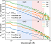 |
Fig. A.1. Simulated escaping spectra from our reprocessing model, with free-free opacity and emission on and off for the spectra drawn with a solid or dashed line respectively. All spectra have Ṁacc = 24 ṀEdd and ρscale = 1. The top and bottom panels have Linj = 16 × 1045 and 2 × 1045 erg s−1 respectively. The 50° and 70° spectra have been scaled by a factor of 0.1 and 5 respectively, to improve visual clarity. The spectral regions covered by UVO and IR observations are indicated by the blue and red shading respectively. |
In high ionisation states, for example, for a lower inclination angle of θ = 50° and a large Linj = 16 L45, the gas is highly ionised and hot. The contribution from free-free emission in these cases is weak, as it scales with temperature as T−7/2 according to Kramers’ law. Therefore, all opacity and emission terms are weak, and electron scattering is dominant. The injected radiation interacts with the outflowing wind, and bulk scattering (adiabatic work) stretches the initial blackbody spectrum, resulting in a blackbody-like slope in the IR. By contrast, in low ionisation states, for example, a larger inclination angle of θ = 70° and a low Linj = 2 L45, bound-free processes dominate, free-free emission makes only a minor contribution, and the spectral is again blackbody-like. For the θ = 70° case, the free-free emission is low due to a low level of ionisation, even when Linj is large, so that there can never be a large IR excess. When the ionisation state is intermediate between the two extremes, for example, for θ = 60° and Linj = 16 L45 or θ = 50° and Linj = 2 L45 we can see that the free-free emission contribution can be very significant.
Appendix B: Additional IR echo modelling
Here we present some additional IR echo models. First, we consider the case in which the TDE evaporates dust out to a certain radius (Rsub), leaving a a spatially thin spherical shell of dust at that radius. The IR echo signal will be dominated by the emission arising at the inner part of the dust distribution, where the dust is hottest, the density highest and the IR echo has a shorter duration, due to shorter light travel times, so the spatially thin shell is a reasonable approximation. The results of our temperature fitting in Sect. 3.2 indicated that if the IR echo model is applicable, the temperature of the dust at early times is ∼2100 K. This is approximately the sublimation temperature for graphite, and is too high for the survival of silicates, so we assume that the dust is pure graphite and consider both a single grain size distribution of 0.1 μm grains and a multiple grain size distribution with minimum size 0.005 μm, number density of grains following a−3.5, and maximum size 0.1 μm. Assuming based on the SED fitting that the dust sublimation temperature is 2100 K, we make use of Eq. (6) to find that the resulting evaporation radii are Revap, single = 0.037 pc and Revap, multiple = 0.064 pc for the single and multiple grain size distributions, respectively. These are lower limits for the sublimation radius, as any additional extreme-UV or X-ray emission from the TDE compared to our assumed blackbody spectrum will contribute to evaporating dust to a larger radius. We then use Eqn. 5 to derive the IR echo behaviour for these radii and dust compositions. We show the result for the single and multiple grain size distributions in Fig. B.1. The resulting IR echoes do not fit the early time emission well. The time evolution in the NIR is not well reproduced, although there are significant systematic uncertainties introduced by subtracting the estimated TDE contribution in the IR, and the MIR data are much brighter than predicted. Furthermore, at later times, nearly all the data is fainter than predicted. Thus the simple shell model cannot reproduce the IR emission we observe.
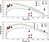 |
Fig. B.1. Top: IR echo model for a spherical shell of graphite dust with a single size composition of 0.1 μm grains. The dust shell has radius 0.037 pc, corresponding to the sublimation radius inferred from the TDE luminosity. Bottom: As top panel, for a multiple size composition with radius 0.064 pc. |
We now consider IR echoes from clumps of dust. To reproduce the early NIR observations, we invoke a clump of dust close to the line of sight, with small enough opening angle that it does not contribute significantly to the observations later than 200 d. For the MIR observations at early times, a more distant clump is required. We show the IR echoes arising from such clumps in Fig. B.2. The early MIR data can be explained with a distant clump with small extent, and the IR echo produced declines fast enough to not contribute to the emission observed at epochs > 200 d. However, the IR echo arising from a nearby clump cannot well explain the early time data. If the clump is placed to well fit the early LC, the clump remains much too luminous compared to the observed NIR data at > 200 d. Minimising the size and proximity to the line of sight for the clump still leaves the IR echo too bright at later times, while also producing a poor fit at the TDE peak.
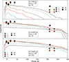 |
Fig. B.2. Top: IR echo model for a small clump of distant dust. This dust can produce the cool dust component observed at 7 d, and declines rapidly enough that it makes no observable contribution to the observed IR SED at later epochs. Middle: IR echo model for a small clump of nearby dust, close to the line of sight. Dust that can reproduce the pre-peak NIR data does not well reproduce the other early NIR data, or the NIR data at ∼200 d. Bottom: IR echo model for a larger clump of nearby dust, further from the line of sight. The NIR data around peak is well reproduced by this configuration, but the IR echo is much too bright to fit the data at > 200 d. |
Appendix C: Additional figures
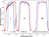 |
Fig. C.1. Normalised JHK transmission curves for SOFI and NOTCam. The atmospheric transmission in the region around the J filter is also shown. |
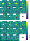 |
Fig. C.2. Subtraction residuals after template subtraction for the unWISE data, with the W1 and W2 band in the upper and lower panels respectively. A linear scaling that shows positive and negative values symmetrically around zero is used to clearly show dipole-like subtraction residuals. White and red circles indicate detections and non-detections, respectively. The radius of the circle corresponds to the FWHM of the image PSF. |
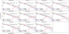 |
Fig. C.3. SED fitting with two blackbodies for the observed UVO+IR SEDs. The fitting was performed with a modified blackbody for the dust. The dust composed of graphite with a variety of grain sizes, as described in Sect. 3.2, including both single size and multiple size distributions. The i band was excluded from the fit. |
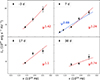 |
Fig. C.4. Power-law fits to the NIR and MIR SEDs of AT 2019azh. The power laws shown in red fit only the NIR data, while those shown in blue fit both the NIR and MIR data. Uncertainties are listed in Table 1. |
Appendix D: Tables
Photometry of AT 2019azh.
All Tables
Results from fitting a power law Lν ∝ να to the IR SEDs observed for AT 2019azh.
All Figures
|
Fig. 1. Photometry of AT 2019azh. The IR photometry is shown with solid coloured symbols, while the extensive UVO photometry is shown using partially transparent symbols. Upper limits are indicated with downward facing triangles. The x-axis is broken as the omitted time period only contains upper limits. The inset plot shows the optical and IR light curves around peak in more detail. |
| In the text | |
|
Fig. 2. SED fitting with two blackbodies (hotter TDE and cooler dust) for the observed UVO+IR SEDs at six epochs (labelled). Fitting was performed with a modified blackbody for the dust. The dust here is entirely composed of graphite with a grain size of 0.1 μm. Empty points are excluded from the fit. |
| In the text | |
|
Fig. 3. Top: SED fitting with two blackbodies (hot TDE and cooler dust) for the observed UVO+IR SED at 7 d. Fitting was performed with a modified blackbody for the dust. The 3.4 μm and 4.6 μm data (open circles) are excluded from the fit, so that a fit with a high dust temperature is preferred. Bottom: SED fitting with three blackbodies (hot TDE and two dust components) at the same epoch, with a modified blackbody corresponding to graphite dust for both dust components. The TDE temperature is fixed. |
| In the text | |
|
Fig. 4. Observed SEDs of AT 2019azh at epochs before 40 d, compared to the grid of simulated escaping spectra. The models have a wavelength grid such that the wavelength changes by 2% at each step, and are smoothed with a median filter of size 3. The top, middle, and bottom panels show models with 50°, 60°, and 70° inclinations, respectively. The colouring denotes the value of Linj as described in the legend, while the solid, dashed, and dotted lines represent models with a density profile scaling factor of 2, 1.5 and 1, respectively. We additionally show the X-ray spectrum observed at 20 d (Guolo et al. 2024) with black circles. |
| In the text | |
|
Fig. 5. As in Fig. 4 but zoomed into the UVO+IR region. The top panel shows the 70° inclination, whereas the other three panels have an inclination of 60°. The density profile scaling is indicated on the panels. |
| In the text | |
|
Fig. 6. Observed SEDs of AT 2019azh, compared with both the best fitting dust models as in Fig. 2, and selected reprocessing models. The SED at 7 d is well fitted by the model with ρscale = 2 and Linj = 16 L45. The models at 17 and 38 d assume that the density and luminosity scale linearly during the decline of the accretion rate. The reduced χ2 values associated with these models are listed in Table 2. |
| In the text | |
|
Fig. 7. Top: IR echo model for a spherical shell of silicate dust. The dust shell has a radius of 0.65 pc, to match the observed photometry between 200 and 400 d. The contribution of the hot TDE blackbody, and any hot dust emission at early times, has been subtracted from the data. The shell does not reproduce the observed drop in the MIR light curves, and under-predicts the potential cool dust component at early times. Bottom: IR echo models for different silicate dust clumps. The dust is at 0.65 pc from the TDE and has θ0 = 30°, 40°, 50°; θclump = 60°, 80°, 100°. The models with larger values of θclump decline at later times. |
| In the text | |
|
Fig. 8. Upper panel: NEOWISE W1 absolute magnitudes for AT 2019azh, alongside the sample of IR-detected TDEs presented in Jiang et al. (2021b). Lower panel: SEDs of TDEs in the literature with IR observations near to the TDEs optical peak. The MIR data are taken from Jiang et al. (2021b) and Swift data are taken from Hinkle et al. (2021b). Optical data for AT 2018hyz, AT 2018dyb, AT 2018zr, and ASASSN-14li are taken from Hung et al. (2020), Holoien et al. (2020), Holoien et al. (2019), and Holoien et al. (2016), respectively. The listed epoch is with respect to peak, except for ASASSN-14li, where it is with respect to the first detection. |
| In the text | |
|
Fig. A.1. Simulated escaping spectra from our reprocessing model, with free-free opacity and emission on and off for the spectra drawn with a solid or dashed line respectively. All spectra have Ṁacc = 24 ṀEdd and ρscale = 1. The top and bottom panels have Linj = 16 × 1045 and 2 × 1045 erg s−1 respectively. The 50° and 70° spectra have been scaled by a factor of 0.1 and 5 respectively, to improve visual clarity. The spectral regions covered by UVO and IR observations are indicated by the blue and red shading respectively. |
| In the text | |
|
Fig. B.1. Top: IR echo model for a spherical shell of graphite dust with a single size composition of 0.1 μm grains. The dust shell has radius 0.037 pc, corresponding to the sublimation radius inferred from the TDE luminosity. Bottom: As top panel, for a multiple size composition with radius 0.064 pc. |
| In the text | |
|
Fig. B.2. Top: IR echo model for a small clump of distant dust. This dust can produce the cool dust component observed at 7 d, and declines rapidly enough that it makes no observable contribution to the observed IR SED at later epochs. Middle: IR echo model for a small clump of nearby dust, close to the line of sight. Dust that can reproduce the pre-peak NIR data does not well reproduce the other early NIR data, or the NIR data at ∼200 d. Bottom: IR echo model for a larger clump of nearby dust, further from the line of sight. The NIR data around peak is well reproduced by this configuration, but the IR echo is much too bright to fit the data at > 200 d. |
| In the text | |
|
Fig. C.1. Normalised JHK transmission curves for SOFI and NOTCam. The atmospheric transmission in the region around the J filter is also shown. |
| In the text | |
|
Fig. C.2. Subtraction residuals after template subtraction for the unWISE data, with the W1 and W2 band in the upper and lower panels respectively. A linear scaling that shows positive and negative values symmetrically around zero is used to clearly show dipole-like subtraction residuals. White and red circles indicate detections and non-detections, respectively. The radius of the circle corresponds to the FWHM of the image PSF. |
| In the text | |
|
Fig. C.3. SED fitting with two blackbodies for the observed UVO+IR SEDs. The fitting was performed with a modified blackbody for the dust. The dust composed of graphite with a variety of grain sizes, as described in Sect. 3.2, including both single size and multiple size distributions. The i band was excluded from the fit. |
| In the text | |
|
Fig. C.4. Power-law fits to the NIR and MIR SEDs of AT 2019azh. The power laws shown in red fit only the NIR data, while those shown in blue fit both the NIR and MIR data. Uncertainties are listed in Table 1. |
| In the text | |
Current usage metrics show cumulative count of Article Views (full-text article views including HTML views, PDF and ePub downloads, according to the available data) and Abstracts Views on Vision4Press platform.
Data correspond to usage on the plateform after 2015. The current usage metrics is available 48-96 hours after online publication and is updated daily on week days.
Initial download of the metrics may take a while.