| Issue |
A&A
Volume 708, April 2026
|
|
|---|---|---|
| Article Number | A82 | |
| Number of page(s) | 22 | |
| Section | Interstellar and circumstellar matter | |
| DOI | https://doi.org/10.1051/0004-6361/202556335 | |
| Published online | 31 March 2026 | |
Molecular diagnostics for the mid-infrared emission of planet-forming disks
Carbon and oxygen elemental abundances
1
Kapteyn Astronomical Institute,
Rijksuniversiteit Groningen, Postbus 800,
9700AV
Groningen,
The Netherlands
2
Leiden Observatory, Leiden University,
2300 RA Leiden,
The Netherlands
3
Max-Planck Institut für Extraterrestrische Physik (MPE),
Giessenbachstr. 1,
85748
Garching,
Germany
4
Space Research Institute, Austrian Academy of Sciences,
Schmiedlstrasse 6,
8042
Graz,
Austria
5
University Observatory, Faculty of Physics, Ludwig-Maximilians-Universität München,
Scheinerstr. 1,
81679
Munich,
Germany
6
Department of Physics and Astronomy, University of Exeter,
Exeter EX4 4QL,
UK
7
Department of Astronomy, University of Michigan,
1085 S. University, Ann Arbor,
MI 48109,
USA
8
Université Paris-Saclay, CNRS,
Institut d’Astrophysique Spatiale,
91405
Orsay,
France
★ Corresponding author: This email address is being protected from spambots. You need JavaScript enabled to view it.
Received:
9
July
2025
Accepted:
17
February
2026
Abstract
Context. Mid-infrared (MIR) observations of planet-forming disks reveal a broad diversity among molecular spectra. Carbon and oxygen abundances play a central role in setting the chemical environment of the inner disk and the spectral appearance.
Aims. We aim to systematically explore how variations in elemental carbon and oxygen abundances affect the MIR spectra of planet-forming disks. We also aim to identify robust MIR molecular diagnostics of the C/H, O/H, and C/O ratios.
Methods. Using the thermochemical disk code ProDiMO and the line radiative transfer code FLiTs, we constructed a grid of 25 models with varying carbon and oxygen abundances, covering a broad range of C/O ratios. We analyzed the resulting MIR molecular emission, including species such as H2O, CO, CO2, C2H2, and OH.
Results. We find that the MIR molecular spectra are highly sensitive not only to the C/O ratio, but also to the absolute abundances of carbon and oxygen. Despite sharing the same disk structure and C/O ratios, the molecular fluxes (e.g., C2H2, CO2) vary by more than an order of magnitude. This variation stems from the differences in excitation conditions and emitting regions caused by the elemental abundances of oxygen and carbon. We identified diagnostic molecular flux ratios (such as CO2/H2O and H2O/C2H2) that can serve as tracers of C/H and O/H, respectively. By combining these diagnostics, we have been able to demonstrate the use of our method for inferring the underlying C/O ratio.
Conclusions. Our model grid provides a framework for interpreting MIR molecular emission from disks, allowing for estimates of elemental abundances if the disk properties and structure are known. Comparisons with recent JWST observations suggest that a variety in C and O abundances is observed in a sample of T Tauri disks, possibly shaped by disk transport processes and the presence of gaps.
Key words: planets and satellites: formation / protoplanetary disks
© The Authors 2026
 Open Access article, published by EDP Sciences, under the terms of the Creative Commons Attribution License (https://creativecommons.org/licenses/by/4.0), which permits unrestricted use, distribution, and reproduction in any medium, provided the original work is properly cited.
This article is published in open access under the Subscribe to Open model. This email address is being protected from spambots. You need JavaScript enabled to view it. to support open access publication.
1 Introduction
The chemical composition of the inner regions of planet-forming disks influences the resulting bulk composition of the forming planets. A quantitative interpretation of observations requires detailed 2D disk modeling. The inner planet-forming regions, typically at temperatures of a few hundred to a thousand Kelvin, emit in the near- to mid-infrared (NIR-MIR) wavelengths. Infrared (IR) observations of T Tauri disks show the presence of CO, one of the most abundant and stable molecules in the innermost regions of disks (Najita et al. 2003; Salyk et al. 2007, 2011a; Brown et al. 2013; Banzatti et al. 2022). The Spitzer Space Telescope revealed a rich chemistry within the inner few astronomical units (au) with numerous detections of species such as H2O, C2H2, HCN, CO2, and OH at MIR wavelengths (Lahuis et al. 2006; Carr & Najita 2008, 2011; Salyk et al. 2008, 2011b; Pascucci et al. 2009, 2013; Pontoppidan et al. 2010; Najita et al. 2010; Kruger et al. 2011; Bast et al. 2013). While these observations have generally indicated water-rich inner regions for T Tauri disks (Salyk et al. 2011b), they also reveal a significant chemical diversity, with some sources showing only CO2 and others primarily showing HCN or C2H2 emission (Pontoppidan et al. 2010). Crucially, some observed nondetections have likely been limited by the sensitivity and spectral resolution of Spitzer.
The Mid-Infrared Instrument (MIRI) on board the James Webb Space Telescope (JWST) significantly improves upon previous observations with its higher sensitivity and spectral resolution. MIRI reveals a greater diversity of the molecular inventory than was observed with Spitzer, detecting fainter molecular features that are important for quantifying the column densities and temperatures of molecules in planet-forming regions (e.g., Kóspál et al. 2023; Grant et al. 2023; Banzatti et al. 2023). For example, molecules such as H2O, OH, C2H2, and HCN, as well as 13CO2, are now detected in the disk around GW Lup (Grant et al. 2023), next to the bright CO2 emission already seen with Spitzer. MIRI also revealed the presence of substantial amounts of warm H2O in a disk with on-going planet formation (Perotti et al. 2023). The high quality spectra allow for a quantitative analysis of molecular band ratios and thermal gradients within the emitting layers (e.g., Gasman et al. 2023; Banzatti et al. 2023; Schwarz et al. 2024; Kaeufer et al. 2024; Temmink et al. 2024a; Romero-Mirza et al. 2024; Temmink et al. 2025).
One of the remarkable outcomes of the MIRI observations is the discovery of unexpectedly carbon-rich chemistry in disks around very low-mass stars (VLMSs) and brown dwarfs (BDs) (Tabone et al. 2023; Arabhavi et al. 2024; Kanwar et al. 2024a; Long et al. 2025; Flagg et al. 2025; Arabhavi et al. 2025a). While earlier Spitzer data hinted at this (Pascucci et al. 2009, 2013), MIRI confirmed and expanded upon this finding, revealing an unprecedented diversity and large column densities (≳ 1020 cm−2) of carbon-bearing molecules in VLMS and BD disks (Tabone et al. 2023; Arabhavi et al. 2024), where the MIR emission of water is generally weaker than that of carbon-bearing molecules (Arabhavi et al. 2025a,b). This contrasts with T Tauri stars, where only one disk with multiple hydrocarbon emission has been identified thus far (Colmenares et al. 2024).
The MIR emission from the inner disks observed by MIRI (e.g., Henning et al. 2024; Pontoppidan et al. 2024) is a complex interplay between the two-dimensional (2D) disk structure, radiative transfer, excitation conditions, and so on. Therefore, tailored modeling studies are the best way to understand how different disk properties and processes affect elemental abundances and MIR spectra in planet-forming disks. Modeling studies have revealed four primary drivers behind the MIR spectral appearance of disks: dust properties, disk structure, radiation fields (stellar and interstellar), and elemental abundances (see Meijerink et al. 2009; Antonellini et al. 2015; Walsh et al. 2015; Woitke et al. 2018; Greenwood et al. 2019; Anderson et al. 2021; Woitke et al. 2024; Vlasblom et al. 2024). In this paper, we focus on the role of elemental abundances.
Gas-phase elemental abundances, particularly the O/H and C/H ratios, are strongly influenced by radial transport processes such as pebble drift and advection of gas, which deliver volatiles such as H2O and CO2 to the inner disk. modifying the abundances by more than an order of magnitude (Bosman et al. 2018; Krijt et al. 2020; Mah et al. 2023). Initially, inward pebble drift significantly increases the oxygen abundances in the inner disk, lowering C/O below solar, a condition that persists briefly (≲ 2 Myr) around VLMSs, but much longer in T Tauri disks (Mah et al. 2023). The depth of disk gaps critically controls the inward delivery of volatiles (Mah et al. 2024). A shallow gap permits early oxygen-rich material flow, which later shifts to elevated C/O as it accretes onto the star, while a moderately deep gap prolongs the inward oxygen delivery and a deep gap entirely restricts volatile delivery, depleting the inner disk of oxygen. The location of the gap relative to the ice-lines of major volatiles strongly influences the inner disk composition and its spectral appearance (Kalyaan et al. 2021, 2023; Sellek et al. 2025). The question of whether such gaps are due to planet formation or to internal photoevaporation can help determine whether the material from the outer disk reaches the inner disk or is carried away by the photoevaporative winds (Lienert et al. 2024). Carbon in dust grains could also be released into the gas phase changing C/H but not O/H (Kress et al. 2010; Anderson et al. 2017; Tabone et al. 2023; Houge et al. 2025).
Trends in observations have been studied to estimate the elemental abundances, particularly carbon and oxygen, and put them in relation to disk parameters. Carr & Najita (2011) and Najita et al. (2013) reported a correlation between the observed HCN/H2O ratio and the submillimeter disk mass, suggesting a link between the inner disk elemental abundances and planet formation. Banzatti et al. (2020) expanded on this and found that the flux ratios, H2O/HCN, H2O/C2H2, and H2O/CO2, decrease with an increase in the outer disk dust radii. They also reported a possible trend between the stellar luminosity-normalized water fluxes and the outer disk radii, which they interpreted as an oxygen-enrichment in the inner disk due to inward pebble transport. The observed C2H2/HCN flux ratios are less than unity in T Tauri disks and greater than unity in VLMS disks (Pascucci et al. 2009; Grant et al. 2025). Using thermochemical disk models, Kanwar et al. (2024a) showed that the high column densities of hydrocarbons in VLMS disks require a C/O ratio greater than 1 (see also Díaz-Berríos et al. 2026). Arabhavi et al. (2025b) also showed that C2H2 fluxes relative to H2O increase with a decrease in stellar luminosities suggesting a higher C/O ratio in sources with lower luminosities (see also Grant et al. 2025).
While the role of disk properties on the MIR emission has been extensively studied, only a handful of studies have investigated how MIR molecular fluxes and their ratios vary with changes in elemental abundances. Najita et al. (2011) showed that in the warm surface layers, the column densities of O-bearing molecules such as H2O, CO2, and OH can decrease and those of C-bearing molecules such as C2H2 and HCN can increase by several orders of magnitude when the C/O ratio changes from 0.2 to 4 when the oxygen abundance is varied. By varying the carbon abundance, Woitke et al. (2018) showed that molecular fluxes such as OH, H2, and ions are relatively stable when the C/O ratio is varied between 0.46 and 1.1, but the fluxes of oxygen-bearing molecules, such as CO2 and H2O, decrease and that of C2H2 increases by up to three orders of magnitude. Similarly, Anderson et al. (2021) reported variations in molecular flux ratios by changing the initial abundance of H2O in the disk, essentially changing the oxygen budget of the disk (i.e., with a C/O ratio between 0.14 and 0.83). These modeling studies vary only one elemental abundance at a time (either carbon or oxygen), but inward material transport by pebble drift and gas advection can enrich or deplete one or both elements.
In this paper, we systematically explored the effect of changing both the carbon and oxygen elemental abundances on the MIR spectra. In Sect. 2, we present the modeling setup and the grid of disk models. The results of the grid are presented in Sect. 3. Reliable molecular diagnostics are presented in Sect. 4 and set in the context of observations and previous modeling studies in Sect. 5. We summarize our conclusions in Sect. 6.
2 The model setup and grid
We used PROtoplanetary DIsk MOdel (ProDiMO1, Woitke et al. 2009; Kamp et al. 2010; Thi et al. 2011; Rab et al. 2018) to simulate disks with different elemental abundances. The code first initializes the physical structure of the disk such as the gas and dust densities, including dust settling. The code then calculates the dust opacities and solves the continuum radiative transfer, thereby determining the dust temperature structure.
Subsequently, the code computes the chemistry and solves the heating & cooling balance to find the molecular abundances and the gas temperature structure. We used Fast Line Tracers (FLiTs, Woitke et al. 2018) to simulate the MIR spectrum from the resulting ProDiMO output. We note that our models are static models and do not include a treatment of radial transport processes.
2.1 Fiducial model
We adopted the fiducial T Tauri disk model of Woitke et al. (2016) and Woitke et al. (2018), incorporating the smooth inner disk edge introduced by Woitke et al. (2024) (also see Appendix A). We adopted the treatment of photorates, molecular shielding, PAHs, dust settling, and escape probabilities from Woitke et al. (2024). The disk model parameters that are common for the entire grid are listed in Table A.1. The dust opacities are explained in Woitke et al. (2016), and based on Min et al. (2016). The opacity calculations assume that the grains are spherical and the materials are well mixed. The refractory dust grains are assumed to be composed of 60% amorphous silicate (Dorschner et al. 1995, Mg0.7Fe0.3SiO3) and 15% amorphous carbon (Zubko et al. 1996), with a porosity of 25%. We use a grain size distribution with grain sizes varying between 0.05 μm and 3 mm with a power-law index of −3.5. While the vertically integrated dust size distribution follows a fixed power law, the model calculates the density-dependent settled dust size distribution following Riols & Lesur (2018). We did not include viscous heating.
We used steady-state chemistry in all the models presented in this paper. Beyond the large DIANA2 chemical network (Kamp et al. 2017), we included the extended hydrocarbon chemical network introduced by Kanwar et al. (2024b). In total, we included 327 species and 13 elements. The elemental abundances of the fiducial model are presented in Table 1. Similarly to Woitke et al. (2018), we include atomic lines, and the rotational and rovibrational molecular transitions in the heating and cooling balance to determine the gas temperatures. The details of the lines included in the MIR wavelength range can be found in Table 2. Species that have collisional data in the LAMDA database or literature (references in Table 2) were treated in local thermodynamic equilibrium (LTE). We note that for many polyatomic molecules, these data are still missing, which is why we chose to use LTE for these cases.
2.2 Grid
The objective of this work is to establish reliable molecular diagnostics for carbon and oxygen abundances and their ratios. Hence, we systematically varied their elemental abundances, while keeping all remaining parameters fixed to those listed in Table A.1. We introduce the Infrared Diagnostics from Line emIssion (IDLI) grid, whereby a uniform set of 25 models is constructed by varying the elemental abundances of carbon and oxygen relative to hydrogen (ε) by −0.5, −0.25, 0.0, 0.25, and 0.5 dex, spanning a total range across one order of magnitude. This range is physically motivated by dynamic transport models (e.g., Ciesla & Cuzzi 2006; Krijt et al. 2020; Mah et al. 2024) and the values explored in previous studies (e.g., Najita et al. 2011; Woitke et al. 2018; Anderson et al. 2021). The parameter space covers C/O ratios higher (up to 4.57) and lower (down to 0.046) than the solar value (0.46, Savage & Sembach 1996). Figure 1 shows the C/O ratio of each model in the grid. In the remainder of the paper, we use (Δ log10(εC), Δ log10(εO)) to refer to a particular model in the grid. For example, the model with a C/O ratio of 0.046 (top-left in Fig. 1) is referred to as (−0.5,0.5). All 5 × 5 panel figures in this paper use the same grid structure, with each panel corresponding to the same carbon and oxygen abundances (and the C/O ratio) as in this figure.
We note that the physical processes that change the elemental abundances in the inner disk not only modify the carbon and oxygen abundances, but also the remaining elements. However, exploring the effect of changes in the other elemental abundances is left to a future work. In this work, we focused on varying the elemental abundances in the whole disk and did not consider radial elemental abundance gradients. This approach is appropriate given that MIR emission originates primarily from the innermost disk regions (within a few au), which are typically well-mixed (Woitke et al. 2022; Semenov et al. 2006).
Elemental abundances in the fiducial model.
Line transitions in the MIRI wavelength range included in the line radiative transfer.
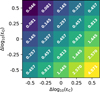 |
Fig. 1 C/O ratios explored in the grid. The change in the carbon and oxygen elemental abundances relative to their fiducial abundances are shown in the x- and y-axes. The fiducial carbon and oxygen elemental abundances are listed in Table 1. Each square represents a model in the grid with the C/O ratio written on the square. The color of the square corresponds to the C/O ratio of the corresponding model. |
3 Results
3.1 Fiducial model
Figure 2 provides the summary of the fiducial disk structure (i.e., model (0,0)). Although we assumed a total disk gas-to-dust mass ratio of 100, the dust settling leaves the upper regions of the disk with gas-to-dust ratios a few orders of magnitude higher. The gas-to-dust mass ratio at the vertical extinction Av=1 layer is about 4200.
The MIR gas emission typically arises from the inner surface regions of the disk (<10 au) with gas temperatures between 1000 K and 300 K (Fig. 2). Below the Av=1 layer, the gas and the dust temperatures are well coupled, whereas above the Av=1 layer, the gas temperatures exceed that of the dust. In this mid-IR gas emission layer, the dominant processes determining the gas temperature are: 1) heating processes such as H2O rovibrational heating, heating by UV photodissociation and PAHs (panel c of Fig. 2); and 2) cooling processes such as H2O rovibrational and rotational cooling, CO rotational and rovibrational cooling, and OH rovibrational cooling (see panel f of Fig. 2).
The continuum-subtracted MIR spectrum of the model between 13 and 17 μm (the molecular-emission-rich part of the spectrum) was convolved to a spectral resolving power of 3000 is shown in Fig. 3. Here, the features of the CO2 Q-branch as well as the P- and R-branches are clearly visible. The C2H2 and HCN emission are quite weak compared to water and CO2. We found strong emission of pure rotational lines of H2O. The spectrum also shows the NeIII atomic fine structure line. We calculated these spectra, including all lines in Table 2 and a proper treatment of opacity overlap using FLiTs. Although we included NH3 and SO2 lines in our model, their emission is a few orders of magnitude smaller than the bright emission shown in Fig. 3. A detailed analysis of SO2 emission can be found in Bethlehem et al. (2025). The spectrum of the fiducial model qualitatively agrees with a typical MIRI observations of T Tauri disks, with brighter H2O and CO2 features than C2H2 and HCN.
3.2 Properties across the grid
The dust temperature, the gas density, and gas-to-dust ratio do not depend on elemental abundances in our models. However, elemental abundances are crucial in calculating the resulting chemistry and the heating-cooling rates, and, thus, the gas temperatures as well. The dominant heating and cooling processes change for different C/O ratios in the grid (also shown in Fig. B.1).
When C/O <1, photodissociation heating becomes prominent in the warm layers (temperatures between 300 K and 1000 K and above Av=1) due to abundant oxygen-bearing molecules such as H2O. The heating by collisional de-excitation of excited H2 also dominates. The dominant cooling processes are rovibrational and rotational water cooling, OH rovibrational cooling, and [OI] line cooling.
When C/O > 1, the photodissociation heating becomes more prominent than in the case of low C/O ratios. Photodissociation heating is largely due to carbon-bearing molecules. There is also a small contribution of carbon photoionisation heating. On the other hand, the dominant cooling processes are C2H2, HCN, and CO rovibrational cooling.
Figure 4 shows the differences in gas temperatures between the models in the grid and the reference model. The gas temperatures below the AV=1 layer do not change with respect to the reference model. This is expected because the gas and dust are in thermal equilibrium in these regions, as seen in the middle panels of Fig. 2; hence, the elemental abundances have little influence. The figure shows that the disk layers above a gas temperature of 1000 K are generally much cooler when the oxygen abundances are higher than the reference model (top two rows of panels), whereas they are warmer when oxygen is depleted (bottom two rows of panels). This is due to the efficient cooling by neutral oxygen in the models with enhanced oxygen abundances (see Fig. B.1).
The diagonal from bottom-left to top-right corresponds to models with the same C/O ratio, but different carbon and oxygen elemental abundances. Along these diagonals, the models with higher oxygen content are slightly cooler in the MIR emitting layer (i.e., between the 300−1000 K contours, above Av=1). This region expands slightly with higher oxygen abundances and shrinks with lower oxygen abundances. This is again due to the dominant cooling processes being H2O and OH cooling. The higher the oxygen abundance, the more efficient H2O and OH cooling become due to their higher abundances. However, the temperature differences are small (<150 K). Similarly, increasing the carbon abundance slightly lowers the temperatures in the MIR emitting layer, as the higher CO abundance leads to more efficient rovibrational cooling (visible in the top two rows). However, when C/O>1, the region below this cooling layer becomes warmer, primarily because the depletion of oxygen reduces the efficiency of H2O cooling. These results show that the elemental abundances can impact the gas temperatures, which, in turn, will also affect the MIR spectra.
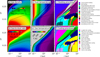 |
Fig. 2 Disk structure of the fiducial model. Only the innermost 12 au and z/r>0.1 region, relevant to MIR emission, is shown. Left panels (a and d) show the gas density and the gas-to-dust mass ratio. Middle panels (b and e) show the dust and the gas temperatures. Right panels (c and f) show the dominant heating and cooling processes, which are labeled to the right of the respective panels. The dotted black line in each panel indicates the vertical extinction Av=1 line. The dashed and dash-dotted black lines show the 300 K and 1000 K gas temperature contours, respectively. The gray contours in panel b indicate the dust temperatures. |
 |
Fig. 3 Continuum subtracted FLiTs spectrum (black, shifted vertically for clarity) of reference model using a spectral resolving power of 3000 between 13 and 17 μm. The different colors indicate different molecular and atomic emission highlighted in colored text. |
4 Molecular diagnostics
In this section, we investigate the resulting MIR spectral appearance across our model grid. Given the established impact of elemental abundances on gas temperatures and chemical abundances, we specifically examine how molecular fluxes and their ratios can serve as diagnostics for these chemical variations.
Table 3 shows the wavelength ranges used to calculated the integrated fluxes used in the following sections. Using different wavelength regions for the pure rotational lines of H2O, for example, 17.19−17.25 μm or 14.485−14.562 μm, does not change the trends presented in this section.
4.1 Abundances and line fluxes across the grid
The strength of the MIR emission of any species depends on the abundance of the species, the excitation condition, and the dust opacity along the line of sight. As we did not vary the dust properties in our models, their impact on the emission strength of molecular lines was only relevant if the emitting regions themselves were varied across the models.
Figure 5 provides an overview of the continuum-subtracted spectra of all models in the grid, limited to the wavelength regions corresponding to emission lines of dominant oxygen and carbon carriers observed in JWST/MIRI observations: the rovibrational emission of CO, H2O, C2H2, and CO2, and the pure rotational emission of H2O. A quantitative comparison of the integrated fluxes of species listed in Table 3 across the grid is shown in Fig. C.2. There is a clear diversity in the range of molecular emission strengths across the grid. Moving along the diagonals (i.e., the models with the same C/O ratios) reveals that the molecular strengths change significantly, although the C/O ratio remains the same (also see Appendix C). To aid the understanding of the diversity in the spectra presented in Fig. 5, it is important to understand the molecular abundances and the line-emitting area of different species (see Figs. D.1–D.5).
Wavelength ranges used for calculating the integrated fluxes of molecules.
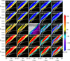 |
Fig. 4 Difference in gas temperatures with respect to the fiducial model. White contours (solid lines) are gas temperatures of 300 K and 1000 K. The white dotted lines show the 300 K and 1000 K gas temperatures, and white dashed lines show Av=1 of the reference model. Since the gas and dust densities are the same for each model, the location of the Av=1 contour is the same in all panels. The center panel shows the actual gas temperature of the fiducial model, which is the same as panel e of Fig. 2. The text in each panel denotes Δ log10(ɛC), Δ log10(ɛO), and the C/O ratio. |
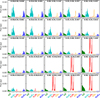 |
Fig. 5 Comparison of molecular emission across the grid. The text in each panel denotes Δ log10(ɛC), Δ log10(ɛO), and the C/O ratio. The molecular spectra are centered at 5.05 μm, 6.6 μm, 13.7 μm, 14.98 μm, and 23.86 μm from left to right. Subscripts ‘rv’ and ‘ro’ refer to rovibrational and pure rotational line emission. |
4.1.1 H2O
The abundance of H2O increases with increasing oxygen abundance, but also increases with decreasing carbon abundance (see Fig. D.1). Correspondingly, the highest water abundance is found in Model (−0.5,0.5), with a C/O ratio of 0.046, and the lowest water abundance is in Model (0.5,−0.5), with a C/O ratio of 4.57. The peak abundance of water in the emitting layers differs by more than three orders of magnitude between these models. Comparing the models with Δ log10(εO)=0 (i.e., for a constant elemental oxygen abundance; see middle panels of Fig. D.1), the emitting region of Models (−0.5,0.0), (−0.25,0.0), and (0.0,0.0) have roughly the same water abundances. However, the water abundance in the same surface region in the Model (0.5,0.0) with C/O>1 is several orders of magnitude lower, even though the model has the same elemental abundance of oxygen. In this model, oxygen is predominantly in the more stable species CO, with CO abundances roughly twice those found in Model (0.0,0.0) (Fig. D.2). Since CO is as abundant as H2O in these emitting layers, doubling the CO abundance takes away most of the oxygen that would otherwise end up in H2O. Inline with the abundances, the water fluxes (both rovibrational and rotational emission) increase with increasing oxygen abundance and decreasing carbon abundance (Fig. 5).
4.1.2 CO
The CO abundances increase with an increase in carbon or oxygen elemental abundances (Fig. D.2). However, the emission strength does not necessarily scale with the CO abundance (see Fig. 5). This is due to the changes in the emitting regions across the models.
For models with C/O<1, the fluxes increase with increasing carbon or oxygen abundances, but only marginally. In models with depleted oxygen abundances, the CO emitting region shifts to slightly higher altitudes in the disk (Fig. D.2). Here, the gas temperatures are higher (>1000 K), but the absolute CO abundances are lower. Conversely, in models with enhanced oxygen, CO emission originates from regions of lower temperature (<1000 K), but higher absolute abundances.
In models with C/O > 1, particularly the models with enhanced carbon (by 0.5 dex), they have much larger emitting areas that probe cooler temperatures, even though neither CO abundances nor the temperature within the emitting regions of these models are the highest in the grid. However, the emitting area is more than five times larger than in models with C/O<1, leading to the strongest CO fluxes in the grid.
4.1.3 C2H2
One of the most prominent trends in the simulated spectra is the bright emission of C2H2 in models with C/O>1 (Fig. 5). In these high C/O models, we find large abundances of C2H2 that form in the disk surface layers (Fig. D.3). While in the rest of the models the emitting region is limited to the innermost regions close to the rim, the C/O> 1 models have emitting areas that are larger by several orders of magnitude.
In models with C/O<1, the C2H2 emission is generally weaker. This is largely because the bulk of the C2H2 resides below the τ=1 layer, leaving little C2H2 that can emit at MIR wavelengths (see Figs. D.3 and D.4). For these models, we find that the emission strength of C2H2 is more strongly influenced by the abundance of oxygen compared to the abundance of carbon. For example, in models with C/O=0.457 (diagonal panels), we see a diversity in the C2H2 emission strengths (Figs. 5 and C.1). Although Model (0.5,0.5) has an order of magnitude higher carbon abundance than Model (−0.5,−0.5), the C2H2 emission is more than an order of magnitude brighter in the latter. This is because oxygen-depletion leads to an increase in C2H2 abundance (also see Estève et al. 2026). The C2H2 abundance in the innermost region above the τ=1 line increases by several orders of magnitude when Δ log10(εO) decreases from +0.5 to −0.5 (top-to-bottom panels Fig. D.4). In addition, the abundance of C2H2 also increases in the thin, radially extended surface layer that also contributes to the observed fluxes. However, the contribution to the total flux from this low density surface layer is less than 33%, even though the emitting area is several orders of magnitude larger. It is not clear whether C2H2 excitation is in LTE in this surface layer, since the densities are on the order of ≥ 1010 cm−3; whereas typical critical densities for these rovibrational lines are ≳ 1012 cm−3. However, IR pumping can also play a role, possibly bringing level populations again closer to LTE.
4.1.4 CO2
Overall, CO2 is the most strongly affected molecule by both carbon and oxygen abundances (Fig. 5). In models with C/O<1, the CO2 emission strength varies by a factor of ∼30. More interestingly, this variation occurs among models of the same C/O (i.e., for models with C/O=0.457).
The abundance of CO2 increases with an increase in the elemental carbon and oxygen abundances (Fig. D.5). On the other hand, the emitting region moves to a cooler region with a decrease in the elemental carbon and oxygen abundances. Both of these together explain the large change in the emission strength across the grid. In models with C/O>1, the CO2 abundances are inherently lower, while the reservoir largely resides below the τ=1 layer.
4.1.5 OH, HCN, Nell, and NH3
The fluxes of OH, HCN, [NeII], and NH3 also display some specific trend (Fig. C.2). Similarly to H2O, OH also peaks when carbon is depleted and oxygen is enhanced. However, the drop in OH flux for models with C/O>1 is not as drastic as in H2O flux, due to the larger emitting area of OH (see Appendix D). It is important to note that while our models include an approximate treatment of NLTE, other processes such as chemical excitation (i.e., prompt emission of OH, Tabone et al. 2021) are not included. This latter excitation mechanism can be very important for predicting accurate emission strengths of OH in disks (e.g., Tabone et al. 2024), but less important for a comparative study between models. The HCN fluxes behave similarly to the C2H2 fluxes, showing high fluxes when C/O>1. The [NeII] emission depends on the oxygen abundance and is only slightly influenced by the carbon abundance. However, the variation is small compared to the other species studied here. The dependence on the oxygen abundance is largely related to the dominant cooling processes in the emitting region of [NeII] (see Appendix D). Finally, NH3 is brighter when the oxygen abundance is higher and carbon abundance is lower. We note that the peak of the brightest NH3 emission in our models is about only 0.2 mJy, largely due to NH3 residing closer to the midplane (z/r<0.15, see Appendix D). We refer to Vlasblom et al. (2026) for a more detailed analysis of NH3 emission.
4.1.6 Summary
Changes in molecular abundances and the properties of the emitting region, such as temperature and spatial extent, are influenced by elemental abundances, leading to variations in the molecular line fluxes. For example, C2H2, which contains no oxygen, is still strongly influenced by the oxygen abundance. Conversely, H2O, which lacks carbon, is affected by both carbon and oxygen abundances. Molecules such as CO and CO2, which include both carbon and oxygen, are influenced by the abundances of both elements; although the effect is more pronounced for CO2. In models where the C/O ratio exceeds 1, the chemistry changes significantly, compared to models with C/O<1, and becomes dominated by hydrocarbons such as C2H2 and depleted in H2O, even when oxygen is not significantly depleted.
4.2 Line flux ratios as tracers of C/O, C/H, and O/H
Figure 5 shows the diversity in the emission strengths of different molecules with the elemental abundances of carbon and oxygen. The figure also shows that for the same C/O ratio, the molecular fluxes (both absolute and relative) can be significantly different.
In the following subsections, we present MIR diagnostics for carbon and oxygen abundances based on line flux ratios. While we have explored ratios involving all species in the model spectra, we mostly focus on a few species for the purposes of this work. Emission from atoms and ions arise from the thin tenuous layers that do not necessarily reflect the bulk composition of the disk, and which are often affected by factors such as disk winds and jets. Molecules such as CO and OH are expected to be excited by LTE processes such as UV and IR pumping, as well as chemical pumping, which go beyond collisional excitation. For example, Temmink et al. (2024b) demonstrated that spectral resolving power higher than that of JWST/MIRI is required to resolve CO lines to uncover the broad and narrow components of CO emission, the latter of which is potentially linked to disk winds. Temmink et al. (2024b) also show that the broad component should arise from within the dust sublimation radius, whereas the bulk of the emission from other molecules arises radially further out in the disk. However, other polyatomic molecules such as CO2, C2H2, H2O (rotational lines), and HCN, which are commonly detected in the MIR spectra of T Tauri disks, have been reproduced sufficiently well with LTE approximation across a wide range of temperatures, column densities, and emitting radii (e.g., Grant et al. 2023; Gasman et al. 2023; Tabone et al. 2023; Banzatti et al. 2023; Xie et al. 2023; Romero-Mirza et al. 2024; Kaeufer et al. 2024; Temmink et al. 2024a, 2025; Vlasblom et al. 2025). Thus, we focus mainly on these molecules (e.g., CO2, C2H2, and H2O).
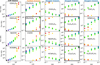 |
Fig. 6 MIR molecular diagnostics: integrated flux ratios. The colors of the scatter points indicate the C/O ratio. All species pairs in our models which show trends are shown. Reliable tracers are highlighted with thick panel edges. |
4.2.1 Tracers of C/O
As noted earlier in this work, the emission of different species react differently to the C/O ratio in the disk. We compared the C/O ratios of all models with the flux ratios between all species in Table 3, as well as [NeII] and H2 S(1), to identify any interesting species pair whose flux ratio can be used to estimate the C/O ratio. We found four flux ratios displays certain trends with the C/O ratio: CO/H2Orv, CO/H2Oro, [NeII]/OH, and HCN/NH3, as shown in the left panels of Fig. 6.
Apart from the flux ratio [NeII]/OH, the remaining three flux ratios increase substantially when the C/O ratios are greater than unity. Below the C/O ratios of unity, the flux ratios show a positive trend with the C/O ratio. For a given C/O ratio (i.e., corresponding to models with different oxygen and carbon abundances), the flux ratios display a minimal spread. However, beyond the C/O ratio of unity, the spread increases and the trend is not quite evident.
These flux ratios are unreliable to be applied to observations. Ro-vibrational band emission of H2O and CO, and OH are influenced by non-LTE effects, and the flux levels of NH3 are below the noise levels of MIRI. So far, NH3 has not been observed in emission in the MIR wavelengths in any planet-forming disks. The strength of the [NeII] emission observed is often influenced by jets and disk winds, and by the X-ray luminosity (Güdel et al. 2010; Pascucci et al. 2020).
4.2.2 Tracers of C/H
Here, we explore tracers for measuring the C/H and O/H individually, so that by combining these tracers, we can determine the C/O ratio. Hence, we go on to compare the C/H ratios (or the elemental carbon abundances) of all models of the grid with the flux ratios between the species, finding four tracers: CO2/H2Orv, CO2/H2Oro, CO/OH, and CO2/OH (Fig. 6). Apart from the flux ratio CO/OH, the remaining three flux ratios are substantially smaller in models with C/O>1, compared to models with C/O<1 for the same carbon abundances. However, in both cases, the flux ratios show a positive trend with the carbon abundance with a small spread. Again, discarding the flux ratios involving the rovibrational band emission of H2O and CO, and OH, we propose the flux ratio between CO2 and pure rotational lines of H2O to be reliable C/H tracer. We note that the two distinct trends of the CO2/H2O ratio (for models with C/O<1 and C/O>1) could theoretically result in degenerate solutions for C/H if the considered abundances are slightly higher or lower than our grid values. However, such degeneracies are lifted when complementary flux ratios are included in the analysis (see Sect. 4.3).
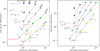 |
Fig. 7 Proposed C/O diagnostics: integrated flux ratios H2O/C2H2 vs. CO2/H2O (left) and CO2/C2H2 vs. CO2/H2O (right). The colors of the scatter points indicate the C/O ratio (see Fig.6). C/O ratio contours are shown as black lines, O/H contours as cyan lines, and C/H contours as red lines. The grey stars indicate the observations. The observed fluxes are taken from Gasman et al. (2025). |
4.2.3 Tracers of O/H
Figure 6 shows several tracers of the elemental oxygen abundance O/H. Again, the flux ratios are substantially different when the C/O ratios are larger than unity. The middle panels of figure corresponding to OH/H2Orv, OH/H2Oro, [NeII]/H2Orv, and HCN/H2Orv show a negative trend with O/H with a small spread when the C/O ratios are smaller than unity. However, each of these flux ratios involve either OH, [NeII], or the rovibrational band emission of H2O.
The remaining oxygen tracers are the flux ratios with C2H2. This is not surprising since, as discussed in Sect. 4.1, the C2H2 emission is strongly influenced by the abundance of oxygen (i.e., O/H). Among these tracers, the flux ratios of the pure rotational lines of H2O and CO2 with C2H2 are reliable. Moreover, the flux ratio CO2/C2H2 has the least spread for a given oxygen abundance.
4.3 Robust diagnostics for measuring C/O
In Sects. 4.2.2 and 4.2.3, we identify reliable tracers of elemental abundances of oxygen and carbon. Since our grid of models are equally spanning the oxygen and carbon abundances as shown in Fig. 1, we expect to reconstruct the matrix in Fig. 1 using these tracers identified.
In Fig. 7, we plot the diagnostic flux ratios with the oxygen tracers on y-axis against the carbon tracer on x-axis: H2O/C2H2 versus CO2/H2O (left) and CO2/C2H2 versus CO2/H2O (right). Models with C/O>1 are not shown in either panels as the oxygen tracer flux ratios of these models lie more than two orders of magnitude lower than the rest (as shown in Figs. 6 and E.1). The ideal case for elemental abundance retrieval would be for the diagnostic grid (Fig. 7) to reproduce the rectangular pattern of abundance variations shown in Fig. 1. However, we find a slightly skewed but still systematically organized grid using these diagnostic tracers. In both panels, both axes span more than an order of magnitude. The black lines, which represent constant C/O ratios, show a relatively clean progression across both panels. This indicates that the combination of these flux ratios is effective in diagnosing the C/O ratio. The cyan and red lines (indicating the constant O/H and C/H values) are somewhat tilted or skewed, but still follow an orderly trend. While the C/H and O/H could not be directly retrieved from the individual flux ratios due to the spread between models of different C/O ratios as shown in Fig. 6, using the combination of their flux ratios allows us to distinguish the elemental abundances.
5 Discussion
5.1 Grid in the context of the observations
In Sect. 4.1, we established that flux ratios that trace the oxygen and carbon abundances can be combined to predict C/O ratios in our models. In this section, we compare the flux ratios from our models to that measured by observations in the MIR. Our models pertain to a single representative disk; whereas in reality, the disk and stellar properties differ from source to source. This can significantly influence the fluxes and flux ratios measured. However, the line ratio diagnostics identified in the previous section span more than an order of magnitude. Even if the model properties do not necessarily reflect the actual source properties, we expect the general trend predicted by our models to be robust.
Figure 7 shows the flux ratios calculated from the fluxes reported by Gasman et al. (2025) for 10 T Tauri disks on top of the model results. Gasman et al. (2025) only included sources with confirmed detections of gaps in millimeter dust. The advantage of using this sample in our comparison is that dynamic disk models indicate that disk gaps can affect the elemental abundances in the inner disk (Kalyaan et al. 2021, 2023; Lienert et al. 2024; Mah et al. 2024; Sellek et al. 2025). Since the MIR fluxes in our models are not affected by the disk geometry beyond a few astronomical units (au) and the smallest gap reported in the sample is about 9 au, we can essentially compare the effect of the varying elemental abundances on the flux ratios. Some caveats are discussed later in this paper.
Figure 7 shows that the range of observed flux ratios that trace the oxygen abundance (CO2/C2H2 and H2Oro/C2H2) spans roughly the same range as our models, but the observed flux ratios that trace the carbon abundance (CO2/H2O) are extended by a factor of 2 below the models with C/O<1. This could largely be due to the specific disk properties of these sources that could be different from those assumed in our models. However, the range of flux ratios show important evidence for difference in elemental abundances in these disks. Sources such as Sz 98, BP Tau and SY Cha show high H2O/C2H2 flux ratios, indicating elevated abundances of oxygen. IQ Tau, and DR Tau correspond roughly to solar oxygen abundance; CI Tau, V1094 Sco, and DL Tau indicate depleted oxygen abundances; and CI Tau, DL Tau, V1094 Sco, and GW Lup have relatively bright CO2 emission, indicating higher carbon abundances than the oxygen-rich sources. With the highest CO2/H2O flux ratio and moderately high H2O/C2H2 ratio, the inner disk of GW Lup could indeed have enhancements in both carbon and oxygen.
While deep gaps completely block the inward transport of material, leaky gaps allow rapid inward transport; both scenarios lead to oxygen depletion in the inner disk (Kalyaan et al. 2021; Mah et al. 2024). In contrast, a moderately leaky gap can prolong the transport process, helping to maintain an oxygen-rich inner disk (Gasman et al. 2025). The sources in the top-left part of Fig. 7 (left panel) are indeed expected to have either moderately leaky gaps or deep gaps where gas has been detected in the gap indicating inward material transport. IQ Tau and DR Tau have similar disk structure (Gasman et al. 2025) and are clustered together in the figure. CI Tau is expected to have a deep gap, while V1094 Sco and DL Tau are expected to be either old disks with moderate gaps or young disks with deep gaps, in either case depleted in oxygen. Interestingly, no source in this sample resides in the top-right part of the figure, indicating equally enhanced carbon and oxygen abundances. GW Lup could, however, still be an example of such enhancement and would require a dedicated thermo-chemical disk model to examine the abundances more accurately. No source has H2O/C2H2 or CO2/C2H2 flux ratios (O/H-tracers) far below the region shown in the figure, which is where our models with C/O>1 lie (see Fig. E.1). A comparison of observations with model fluxes related to Fig. 7, but with observed flux ratios of disks around VLMSs, is provided in Appendix E.
5.2 Comparison to previous modeling studies
Anderson et al. (2021) explored the effects of elemental abundances on MIR fluxes. They adjusted the abundance of H2O to achieve a change in the C/O ratio, essentially changing the oxygen abundances only. According to our analysis, such variation should lead to large changes in molecular flux ratios of the oxygen tracers (H2Oro/C2H2. and.CO2/C2H2), but not so for the carbon tracer (CO2/H2O). Indeed, they reported broad variations in the flux ratios (up to three orders of magnitude) of CO2/C2H2 and H2O/C2H2, but a very slight variation in the CO2/H2O ratio. However, the specific values of these variations do not show a match between the two studies. This could be due to differences in the modeling approaches. For example, we performed a full line radiative transfer solution to predict the model spectra, but Anderson et al. (2021) used LTE slab models to predict the spectra, considering the column of molecules down to a depth where the total H2 gas column densities reach 1.8 × 1023 cm−2 and up to 10 au in radius. We clearly see that for molecules such as H2O, CO, and CO2, only the thin layer on the disk surface, which is radially limited, contributes to the total flux.
Woitke et al. (2018) showed the sensitivity of the fluxes close to a C/O ratio of unity by varying the elemental carbon abundance. They reported a decrease in flux of CO2 and an increase in the flux of C2H2 by several orders of magnitude when pushing models to values of C/O>1; this is in line with our models. However, the relative change in flux of the individual molecules such as H2O, or CO2 in our models are not as drastic as reported by Woitke et al. (2018). This difference could stem from several factors, including slightly different disk structures and different treatments of escape probabilities and shielding (see Woitke et al. 2024). Moreover, Woitke et al. (2018) reported integrated fluxes for all the lines of a molecule.
5.3 Caveats
While observed oxygen tracers align well with our C/O<1 models, the observations do not overlap with the model grid when oxygen and carbon tracers are considered simultaneously. One of the important factors that could affect the CO2/H2O ratio is the inner disk radius. Woitke et al. (2018), Anderson et al. (2021), and Vlasblom et al. (2024) showed that the inner disk radius has a distinct effect on the MIR fluxes. The fluxes increase with an increase in inner radius due to the larger emitting area of the inner rim, but only up to about 5 au ; beyond this point, the fluxes drop due to lower rim temperatures (lines cannot be excited anymore). The fluxes can vary by more than an order of magnitude and this effect depends on the molecule, thereby strongly influencing the CO2/H2O flux ratio. For example, BP Tau is expected to have a close-in gap or a large cavity; the latter could strongly boost the CO2/H2O flux ratio, making it appear water-rich. Vlasblom et al. (2024) showed that variations in the CO2/H2O molecular flux ratio, driven by changes in the inner disk radius, can exceed an order of magnitude; this result is comparable to the range shown in Fig. 7. Woitke et al. (2022) showed that with the same elemental abundances vertical mixing can drive an active organic chemistry, thereby enhancing hydrocarbon fluxes. Variability in the inner disk turbulence between sources can cause a further spread in range of elemental abundances that reproduce the same flux ratios.
Additionally, previous modeling studies have shown that dust properties and disk structures can play a large role in the spectral appearance of the disk, since they determine the amount and shape of radiation field that enters or leaves the disk. For example, the gas-to-dust ratio, maximum dust grain size, dust settling, and the dust size distribution can vary the mid-IR line strengths by more than an order of magnitude (Meijerink et al. 2009; Antonellini et al. 2015; Woitke et al. 2018; Greenwood et al. 2019; Woitke et al. 2024). Furthermore, in this study, we assumed fixed stellar properties. However, the observed sources span stellar luminosities between 0.22−1.52 L⊙. The mass and luminosity of the central object can strongly influence the molecular abundances (Walsh et al. 2015). A stronger UV radiation field (from the star or the interstellar medium) or the presence of X-rays greatly enhances the MIR fluxes (Antonellini et al. 2015; Walsh et al. 2015; Kanwar et al. 2026).
Although multiple additional factors can influence the predicted fluxes and flux ratios, the change seen among the elemental abundances in our grid largely explains the spectral diversity of the observations. More detailed analyses are required, taking into account the source specific properties to constrain the elemental abundances in individual sources.
6 Conclusions
We constructed a grid of thermochemical disk models that vary both the carbon and oxygen elemental abundances, allowing for a systematic exploration of their combined effects on MIR molecular emission. Our key findings are as follows:
Nonuniqueness of the C/O ratio: Molecular fluxes and ratios cannot be solely attributed to the C/O ratio; models with identical C/O ratios, but different absolute C and O abundances can yield significantly different spectra;
Sensitivity of individual species: Molecules such as H2O, C2H2, and CO2 are particularly sensitive to the elemental abundance of carbon and/or oxygen. Notably, C2H2 is, in fact, a purely carbon-bearing molecule, but it is strongly affected by oxygen depletion, while H2O and CO2 are influenced by both elements;
Diagnostic tracers: We identified flux ratios that serve as diagnostics for elemental C/H (e.g., CO2/H2O), O/H (e.g., H2O/C2H2) abundances and, thus, indirectly measuring the C/O ratio. These tracers are based on species and spectral regions accessible to JWST/MIRI observations;
Application to observations: When compared with recent observations of T Tauri disks with confirmed dust gaps, our diagnostic flux ratios reveal evidence of varying carbon and oxygen enrichment across sources (below C/O of 1), highlighting the role of transport processes such as radial drift and disk gaps.
Acknowledgements
We thank the Center for Information Technology of the University of Groningen for their support and for providing access to the Hábrók high performance computing cluster. I.K., A.M.A., and E.v.D. acknowledge support from grant TOP-1 614.001.751 from the Dutch Research Council (NWO). T.K. acknowledges support from STFC Grant ST/Y002415/1.
References
- Anderson, D. E., Bergin, E. A., Blake, G. A., et al. 2017, ApJ, 845, 13 [NASA ADS] [CrossRef] [Google Scholar]
- Anderson, D. E., Blake, G. A., Cleeves, L. I., et al. 2021, ApJ, 909, 55 [NASA ADS] [CrossRef] [Google Scholar]
- Antonellini, S., Kamp, I., Riviere-Marichalar, P., et al. 2015, A&A, 582, A105 [NASA ADS] [CrossRef] [EDP Sciences] [Google Scholar]
- Arabhavi, A. M., Kamp, I. Henning, T., & van Dishoeck, E. F., 2024, Science, 7, 805 [Google Scholar]
- Arabhavi, A. M., Kamp, I., Henning, T., et al. 2025a, A&A, 699, A194 [NASA ADS] [CrossRef] [EDP Sciences] [Google Scholar]
- Arabhavi, A. M., Kamp, I., van Dishoeck, E. F., et al. 2025b, ApJ, 984, L62 [Google Scholar]
- Banzatti, A., Pascucci, I., Bosman, A. D., et al. 2020, ApJ, 903, 124 [NASA ADS] [CrossRef] [Google Scholar]
- Banzatti, A., Abernathy, K. M., Brittain, S., et al. 2022, AJ, 163, 174 [NASA ADS] [CrossRef] [Google Scholar]
- Banzatti, A., Pontoppidan, K. M., Carr, J. S., et al. 2023, ApJ, 957, L22 [NASA ADS] [CrossRef] [Google Scholar]
- Bast, J. E., Lahuis, F., van Dishoeck, E. F., & Tielens, A. G. G. M., 2013, A&A, 551, A118 [NASA ADS] [CrossRef] [EDP Sciences] [Google Scholar]
- Bethlehem, J., Kamp, I., et al. 2025, A&A, submitted [Google Scholar]
- Bosman, A. D., Tielens, A. G. G. M., & van Dishoeck, E. F., 2018, A&A, 611, A80 [NASA ADS] [CrossRef] [EDP Sciences] [Google Scholar]
- Brooke, J. S. A., Bernath, P. F., Western, C. M., et al. 2016, J. Quant. Spec. Radiat. Transf., 168, 142 [NASA ADS] [CrossRef] [Google Scholar]
- Brown, J. M., Pontoppidan, K. M., van Dishoeck, E. F., et al. 2013, ApJ, 770, 94 [NASA ADS] [CrossRef] [Google Scholar]
- Carr, J. S., & Najita, J. R., 2008, Science, 319, 1504 [Google Scholar]
- Carr, J. S., & Najita, J. R., 2011, ApJ, 733, 102 [NASA ADS] [CrossRef] [Google Scholar]
- Ciesla, F. J., & Cuzzi, J. N., 2006, Icarus, 181, 178 [NASA ADS] [CrossRef] [Google Scholar]
- Colmenares, M. J., Bergin, E. A., Salyk, C., et al. 2024, ApJ, 977, 173 [NASA ADS] [CrossRef] [Google Scholar]
- Dere, K. P., Landi, E., Mason, H. E., Monsignori Fossi, B. C., & Young, P. R., 1997, A&AS, 125, 149 [Google Scholar]
- Díaz-Berríos, J. K., Walsh, C., & van Dishoeck, E. F. 2026, arXiv e-prints [arXiv:2601.23069] [Google Scholar]
- Dorschner, J., Begemann, B., Henning, T., Jaeger, C., & Mutschke, H., 1995, A&A, 300, 503 [Google Scholar]
- Estève, P., Tabone, B., Habart, E., et al. 2026, A&A, submitted [Google Scholar]
- Flagg, L., Scholz, A., Almendros-Abad, V., et al. 2025, ApJ, 986, 200 [Google Scholar]
- Gasman, D., van Dishoeck, E. F., Grant, S. L., et al. 2023, A&A, 679, A117 [NASA ADS] [CrossRef] [EDP Sciences] [Google Scholar]
- Gasman, D., Temmink, M., van Dishoeck, E. F., et al. 2025, A&A, 694, A147 [NASA ADS] [CrossRef] [EDP Sciences] [Google Scholar]
- Gordon, I. E., Rothman, L. S., Hargreaves, R. J., et al. 2022, J. Quant. Spec. Radiat. Transf., 277, 107949 [NASA ADS] [CrossRef] [Google Scholar]
- Grant, S. L., van Dishoeck, E. F., Tabone, B., et al. 2023, ApJ, 947, L6 [NASA ADS] [CrossRef] [Google Scholar]
- Grant, S. L., Temmink, M., van Dishoeck, E. F., et al. 2025, A&A, 702, A126 [NASA ADS] [CrossRef] [EDP Sciences] [Google Scholar]
- Greenwood, A. J., Kamp, I., Waters, L. B. F. M., Woitke, P., & Thi, W. F., 2019, A&A, 631, A81 [NASA ADS] [CrossRef] [EDP Sciences] [Google Scholar]
- Güdel, M., Lahuis, F., Briggs, K. R., et al. 2010, A&A, 519, A113 [CrossRef] [EDP Sciences] [Google Scholar]
- Henning, T., Kamp, I., Samland, M., et al. 2024, PASP, 136, 054302 [NASA ADS] [CrossRef] [Google Scholar]
- Houge, A., Johansen, A., Bergin, E., et al. 2025, A&A, 699, A227 [NASA ADS] [CrossRef] [EDP Sciences] [Google Scholar]
- Kaeufer, T., Min, M., Woitke, P., Kamp, I., & Arabhavi, A. M., 2024, A&A, 687, A209 [NASA ADS] [CrossRef] [EDP Sciences] [Google Scholar]
- Kalyaan, A., Pinilla, P., Krijt, S., Mulders, G. D., & Banzatti, A., 2021, ApJ, 921, 84 [CrossRef] [Google Scholar]
- Kalyaan, A., Pinilla, P., Krijt, S., et al. 2023, ApJ, 954, 66 [NASA ADS] [CrossRef] [Google Scholar]
- Kamp, I., Tilling, I., Woitke, P., Thi, W. F., & Hogerheijde, M., 2010, A&A, 510, A18 [NASA ADS] [CrossRef] [EDP Sciences] [Google Scholar]
- Kamp, I., Thi, W. F., Woitke, P., et al. 2017, A&A, 607, A41 [NASA ADS] [CrossRef] [EDP Sciences] [Google Scholar]
- Kanwar, J., Kamp, I., Jang, H., et al. 2024a, A&A, 689, A231 [NASA ADS] [CrossRef] [EDP Sciences] [Google Scholar]
- Kanwar, J., Kamp, I., Woitke, P., et al. 2024b, A&A, 681, A22 [NASA ADS] [CrossRef] [EDP Sciences] [Google Scholar]
- Kanwar, J., Kamp, I., Woitke, P., et al. 2026, A&A, 705, A222 [NASA ADS] [CrossRef] [EDP Sciences] [Google Scholar]
- Kóspál, Á., Ábrahám, P., Diehl, L., et al. 2023, ApJ, 945, L7 [CrossRef] [Google Scholar]
- Kramida, A., Yu. Ralchenko, Reader, J., & NIST ASD Team 2024, NIST Atomic Spectra Database (ver. 5.12), [Online]. Available: http://www.physics.nist.gov/asd [2025, July 5]. National Institute of Standards and Technology, Gaithersburg, MD [Google Scholar]
- Kress, M. E., Tielens, A. G. G. M., & Frenklach, M., 2010, Adv. Space Res., 46, 44 [NASA ADS] [CrossRef] [Google Scholar]
- Krijt, S., Bosman, A. D., Zhang, K., et al. 2020, ApJ, 899, 134 [NASA ADS] [CrossRef] [Google Scholar]
- Kruger, A. J., Richter, M. J., Carr, J. S., et al. 2011, ApJ, 729, 145 [Google Scholar]
- Lahuis, F., van Dishoeck, E. F., Boogert, A. C. A., et al. 2006, ApJ, 636, L145 [NASA ADS] [CrossRef] [Google Scholar]
- Lienert, J. L., Bitsch, B., & Henning, T., 2024, A&A, 691, A72 [NASA ADS] [CrossRef] [EDP Sciences] [Google Scholar]
- Lique, F., 2015, MNRAS, 453, 810 [NASA ADS] [CrossRef] [Google Scholar]
- Long, F., Pascucci, I., Houge, A., et al. 2025, ApJ, 978, L30 [Google Scholar]
- Mah, J., Bitsch, B., Pascucci, I., & Henning, T., 2023, A&A, 677, L7 [CrossRef] [EDP Sciences] [Google Scholar]
- Mah, J., Savvidou, S., & Bitsch, B., 2024, A&A, 686, L17 [NASA ADS] [CrossRef] [EDP Sciences] [Google Scholar]
- Meijerink, R., Pontoppidan, K. M., Blake, G. A., Poelman, D. R., & Dullemond, C. P., 2009, ApJ, 704, 1471 [Google Scholar]
- Min, M., Rab, C., Woitke, P., Dominik, C., & Ménard, F., 2016, A&A, 585, A13 [NASA ADS] [CrossRef] [EDP Sciences] [Google Scholar]
- Najita, J., Carr, J. S., & Mathieu, R. D., 2003, ApJ, 589, 931 [NASA ADS] [CrossRef] [Google Scholar]
- Najita, J. R., Carr, J. S., Strom, S. E., et al. 2010, ApJ, 712, 274 [NASA ADS] [CrossRef] [Google Scholar]
- Najita, J. R., Ádámkovics, M., & Glassgold, A. E., 2011, ApJ, 743, 147 [NASA ADS] [CrossRef] [Google Scholar]
- Najita, J. R., Carr, J. S., Pontoppidan, K. M., et al. 2013, ApJ, 766, 134 [Google Scholar]
- Pascucci, I., Apai, D., Luhman, K., et al. 2009, ApJ, 696, 143 [Google Scholar]
- Pascucci, I., Herczeg, G., Carr, J. S., & Bruderer, S., 2013, ApJ, 779, 178 [NASA ADS] [CrossRef] [Google Scholar]
- Pascucci, I., Banzatti, A., Gorti, U., et al. 2020, ApJ, 903, 78 [Google Scholar]
- Perotti, G., Christiaens, V., Henning, T., et al. 2023, Nature, 620, 516 [NASA ADS] [CrossRef] [Google Scholar]
- Perotti, G., Kurtovic, N. T., Henning, T., et al. 2026, ApJ, 997, 281 [Google Scholar]
- Pontoppidan, K. M., Salyk, C., Blake, G. A., et al. 2010, ApJ, 720, 887 [CrossRef] [Google Scholar]
- Pontoppidan, K. M., Salyk, C., Banzatti, A., et al. 2024, ApJ, 963, 158 [NASA ADS] [CrossRef] [Google Scholar]
- Rab, C., Güdel, M., Woitke, P., et al. 2018, A&A, 609, A91 [NASA ADS] [CrossRef] [EDP Sciences] [Google Scholar]
- Rahmann, U., Kreutner, W., & Kohse-Höinghaus, K., 1999, Appl. Phys. B: Lasers Opt., 69, 61 [NASA ADS] [CrossRef] [Google Scholar]
- Riols, A., & Lesur, G., 2018, A&A, 617, A117 [NASA ADS] [CrossRef] [EDP Sciences] [Google Scholar]
- Romero-Mirza, C. E., Banzatti, A., Öberg, K. I., et al. 2024, ApJ, 975, 78 [NASA ADS] [CrossRef] [Google Scholar]
- Salyk, C., Blake, G. A., Boogert, A. C. A., & Brown, J. M., 2007, ApJ, 655, L105 [NASA ADS] [CrossRef] [Google Scholar]
- Salyk, C., Pontoppidan, K. M., Blake, G. A., et al. 2008, ApJ, 676, L49 [NASA ADS] [CrossRef] [Google Scholar]
- Salyk, C., Blake, G. A., Boogert, A. C. A., & Brown, J. M. 2011a, ApJ, 743, 112 [NASA ADS] [CrossRef] [Google Scholar]
- Salyk, C., Pontoppidan, K. M., Blake, G. A., Najita, J. R., & Carr, J. S. 2011b, ApJ, 731, 130 [Google Scholar]
- Savage, B. D., & Sembach, K. R., 1996, ARA&A, 34, 279 [Google Scholar]
- Schöier, F. L., van der Tak, F. F. S., van Dishoeck, E. F., & Black, J. H., 2005, A&A, 432, 369 [Google Scholar]
- Schwarz, K. R., Henning, T., Christiaens, V., et al. 2024, ApJ, 962, 8 [NASA ADS] [CrossRef] [Google Scholar]
- Sellek, A. D., Vlasblom, M., & van Dishoeck, E. F., 2025, A&A, 694, A79 [NASA ADS] [CrossRef] [EDP Sciences] [Google Scholar]
- Semenov, D., Wiebe, D., & Henning, T., 2006, ApJ, 647, L57 [NASA ADS] [CrossRef] [Google Scholar]
- Tabone, B., van Hemert, M. C., van Dishoeck, E. F., & Black, J. H., 2021, A&A, 650, A192 [NASA ADS] [CrossRef] [EDP Sciences] [Google Scholar]
- Tabone, B., Bettoni, G., van Dishoeck, E. F., et al. 2023, Nat. Astron., 7, 805 [NASA ADS] [CrossRef] [Google Scholar]
- Tabone, B., van Dishoeck, E. F., & Black, J. H., 2024, A&A, 691, A11 [NASA ADS] [CrossRef] [EDP Sciences] [Google Scholar]
- Temmink, M., van Dishoeck, E. F., Gasman, D., et al. 2024a, A&A, 689, A330 [NASA ADS] [CrossRef] [EDP Sciences] [Google Scholar]
- Temmink, M., van Dishoeck, E. F., Grant, S. L., et al. 2024b, A&A, 686, A117 [NASA ADS] [CrossRef] [EDP Sciences] [Google Scholar]
- Temmink, M., Sellek, A. D., Gasman, D., et al. 2025, A&A, 699, A134 [NASA ADS] [CrossRef] [EDP Sciences] [Google Scholar]
- Thi, W. F., Woitke, P., & Kamp, I., 2011, MNRAS, 412, 711 [Google Scholar]
- Thi, W. F., Kamp, I., Woitke, P., et al. 2013, A&A, 551, A49 [NASA ADS] [CrossRef] [EDP Sciences] [Google Scholar]
- Vlasblom, M., van Dishoeck, E. F., Tabone, B., & Bruderer, S., 2024, A&A, 682, A91 [NASA ADS] [CrossRef] [EDP Sciences] [Google Scholar]
- Vlasblom, M., Temmink, M., Grant, S. L., et al. 2025, A&A, 693, A278 [NASA ADS] [CrossRef] [EDP Sciences] [Google Scholar]
- Vlasblom, M., Arabhavi, A. M., de Klerk, N., et al. 2026, ACS Earth Space Chem., submitted [Google Scholar]
- Walsh, C., Nomura, H., & van Dishoeck, E., 2015, A&A, 582, A88 [NASA ADS] [CrossRef] [EDP Sciences] [Google Scholar]
- Wiese, W. L., Fuhr, J. R., & Deters, T. M., 1996, Atomic transition probabilities of carbon, nitrogen, and oxygen: a critical data compilation [Google Scholar]
- Woitke, P., Kamp, I., & Thi, W. F., 2009, A&A, 501, 383 [NASA ADS] [CrossRef] [EDP Sciences] [Google Scholar]
- Woitke, P., Min, M., Pinte, C., et al. 2016, A&A, 586, A103 [NASA ADS] [CrossRef] [EDP Sciences] [Google Scholar]
- Woitke, P., Min, M., Thi, W. F., et al. 2018, A&A, 618, A57 [NASA ADS] [CrossRef] [EDP Sciences] [Google Scholar]
- Woitke, P., Arabhavi, A. M., Kamp, I., & Thi, W. F., 2022, A&A, 668, A164 [NASA ADS] [CrossRef] [EDP Sciences] [Google Scholar]
- Woitke, P., Thi, W. F., Arabhavi, A. M., et al. 2024, A&A, 683, A219 [NASA ADS] [CrossRef] [EDP Sciences] [Google Scholar]
- Wrathmall, S. A., Gusdorf, A., & Flower, D. R., 2007, MNRAS, 382, 133 [NASA ADS] [CrossRef] [Google Scholar]
- Xie, C., Pascucci, I., Long, F., et al. 2023, ApJ, 959, L25 [NASA ADS] [CrossRef] [Google Scholar]
- Zubko, V. G., Mennella, V., Colangeli, L., & Bussoletti, E., 1996, MNRAS, 282, 1321 [Google Scholar]
Version 8dedaadb, https://prodimo.iwf.oeaw.ac.at/
Disk Analysis, https://diana.iwf.oeaw.ac.at/
Appendix A Fiducial model and non-LTE OH data
The disk model parameters that remain common through out the grid are listed in Table A.1. The physical structure of the disk follows the model of Woitke et al. (2016), incorporating the smooth inner disk edge and density structure from Eq. (71) of Woitke et al. (2024). Including this smooth edge is crucial for accurately predicting MIR emission from the inner disk (Woitke et al. 2024; Henning et al. 2024).
In this work, we use an OH line list, encompassing levels and radiative transitions for v=0 and v=1 (N ≤ 54 and N ≤ 50 for v=0 and 1, respectively), based on Brooke et al. (2016). The collision rates with o−H2 and p−H2 between pure rotational levels in the LAMDA database (Schöier et al. 2005) served as the basis to estimate all the missing rates. The methodology follows Tabone et al. (2024) for the expansion of the v=0 rates. Since we considered collisional rates between normal H2 and OH, the rates with o−H2 and p−H2 have been merged into a single set of normal- H2 assuming a constant H2 ortho-to-para ratio of 3:1. The rates have been further extrapolated for transitions arising from higher rotational levels and temperatures up to 2000 K assuming that rates γ ∝ exp (−Δ E/k T), where Δ E is the energy difference between two levels, k. The collision rates from levels arising from v=1 were computed using the equal probability method and the coefficients in Rahmann et al. (1999). In this study, we did not consider other potential collision partners.
Common disk model parameters.
Appendix B Heating and cooling
A comparison of the dominant heating and cooling processes for five models of different C/O ratios are presented in Fig. B.1.
Appendix C Diverse spectral appearance with the same C/O ratio
Figure C.1 shows the spectra of five models from the grid that have the same C/O ratio, but different abundances of carbon and oxygen. The spectra are diverse, varying between spectra dominated by CO2, H2O, or C2H2, all for the same C/O ratio. Figure C.2 presents a quantitative comparison of integrated molecular fluxes of different species, each normalized to the flux from the fiducial model.
Appendix D Abundances and emitting regions different species
Figures D.1-D.9 show the abundances of the species discussed in this paper. H2O, CO, C2H2, and CO2 are discussed in the main text (Sect. 4.1). The line-emitting regions are bounded by four contours. The upper and lower boundaries indicate the 15% and 85% levels of the local vertical flux (integrated from the surface to the midplane). The vertical lines mark the radii where the radially cumulative flux reaches 15% and 85% of the total emission. Together, these boundaries enclose approximately 50% of the total line flux (also see Woitke et al. 2016). We calculate the flux contribution of individual grid points using the escape probability formalism presented in Sect. 2.2 of Woitke et al. (2024).
Figure D.6 shows the abundances and the line emitting regions of OH. Clearly, higher oxygen abundances lead to higher OH abundances. The emitting region morphs from a thin-long layer to a thick-narrow layer with increasing oxygen abundances. The temperature of the emitting region also moves slightly higher up and lower down around the 1000 K contour with changing oxygen abundance.
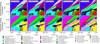 |
Fig. B.1 Dominant heating and cooling processes across models of different C/O ratios. The white dashed lines indicate the 300 K and 1000 K gas temperature contours. The white dotted lines indicate the Av=1 line. |
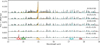 |
Fig. C.1 FLiTs spectra of five models with the same C/O ratio of 0.45, but different C/H and O/H (indicated in the figure). The spectrum in the center is the fiducial model (0,0). |
Figure D.7 shows that the abundances and the line emitting regions of HCN behave similar to C2H2. When C/O<1, the emitting region is a narrow layer above the τ=1 line. The abundances in the surface layer increase with decreasing oxygen abundance. The abundances increases significantly when the C/O ratio is greater than 1 and the emitting region extends to much larger areas.
Figure D.8 shows the abundances and the line-emitting regions of NH3. The NH3 reservoir is largely limited to the region below the τ=1 layer. The low abundances above this layer and the very narrow emitting region lead to small fluxes.
Figure D.9 shows the abundances and the line-emitting regions of [NeII]. The Ne+ reservoir is largely limited to the high temperature region above 1000 K. Since Ne+ is inert, the abundances do not change with carbon and oxygen abundances. However, the emitting regions change slightly in response to changes in the temperature structure of the gas.
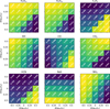 |
Fig. C.2 Integrated fluxes normalized to the fiducial model. |
Appendix E C/O diagnostics with VLMSs
Similarly to Fig. 7, Fig. E.2 presents the observed molecular flux ratios of disks around 11 VLMSs, which are generally carbon-rich, in comparison with those of the models. These sources are taken from Arabhavi et al. (2025a) with one source from Xie et al. (2023). The observations generally fall outside the flux ratios traced by the models. J0438 (highly inclined) and Sz114 have a water-rich MIRI spectra (Perotti et al. 2026; Arabhavi et al. 2025b; Xie et al. 2023). Comparing the model flux ratios to the observed flux ratios of J0438 and Sz114 indicates C/O ratios less than 1. All the other sources have multiple bright hydrocarbon emission corresponding to C/O ratios greater than 1 (Arabhavi et al. 2025a; Kanwar et al. 2024a). In fact, Kanwar et al. (2026) show that models require a C/O ratio significantly larger than unity to reproduce the C2H2 pseudo-continuum observed in J1605. Moreover, not much is known about the inner and outer disk structures of these carbon-rich sources.
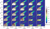 |
Fig. D.1 Abundance and line emitting region (red line) of H2O. The solid black lines indicate the gas temperatures of 300 K and 1000 K, the dotted line indicates the |


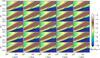 |
Fig. D.9 Same as Fig. D.1, but for Ne+. The dashed line indicates the τ[NeII]=1 line. Note the different axes limits. |
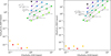 |
Fig. E.1 Same as Fig. 7, but including models with C/O>1. The colors of the points correspond to the C/O ratios (see Fig. 6). The models with C/O>1 are at the bottom-left corner of each panel. |
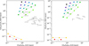 |
Fig. E.2 Same as Fig. 7, but for observations of disks around VLMSs, and the wavelength intervals are adapted for these sources. The spectra and detections are taken from Arabhavi et al. (2025a), Arabhavi et al. (2025b), and Xie et al. (2023). |
All Tables
Line transitions in the MIRI wavelength range included in the line radiative transfer.
All Figures
|
Fig. 1 C/O ratios explored in the grid. The change in the carbon and oxygen elemental abundances relative to their fiducial abundances are shown in the x- and y-axes. The fiducial carbon and oxygen elemental abundances are listed in Table 1. Each square represents a model in the grid with the C/O ratio written on the square. The color of the square corresponds to the C/O ratio of the corresponding model. |
| In the text | |
|
Fig. 2 Disk structure of the fiducial model. Only the innermost 12 au and z/r>0.1 region, relevant to MIR emission, is shown. Left panels (a and d) show the gas density and the gas-to-dust mass ratio. Middle panels (b and e) show the dust and the gas temperatures. Right panels (c and f) show the dominant heating and cooling processes, which are labeled to the right of the respective panels. The dotted black line in each panel indicates the vertical extinction Av=1 line. The dashed and dash-dotted black lines show the 300 K and 1000 K gas temperature contours, respectively. The gray contours in panel b indicate the dust temperatures. |
| In the text | |
|
Fig. 3 Continuum subtracted FLiTs spectrum (black, shifted vertically for clarity) of reference model using a spectral resolving power of 3000 between 13 and 17 μm. The different colors indicate different molecular and atomic emission highlighted in colored text. |
| In the text | |
|
Fig. 4 Difference in gas temperatures with respect to the fiducial model. White contours (solid lines) are gas temperatures of 300 K and 1000 K. The white dotted lines show the 300 K and 1000 K gas temperatures, and white dashed lines show Av=1 of the reference model. Since the gas and dust densities are the same for each model, the location of the Av=1 contour is the same in all panels. The center panel shows the actual gas temperature of the fiducial model, which is the same as panel e of Fig. 2. The text in each panel denotes Δ log10(ɛC), Δ log10(ɛO), and the C/O ratio. |
| In the text | |
|
Fig. 5 Comparison of molecular emission across the grid. The text in each panel denotes Δ log10(ɛC), Δ log10(ɛO), and the C/O ratio. The molecular spectra are centered at 5.05 μm, 6.6 μm, 13.7 μm, 14.98 μm, and 23.86 μm from left to right. Subscripts ‘rv’ and ‘ro’ refer to rovibrational and pure rotational line emission. |
| In the text | |
|
Fig. 6 MIR molecular diagnostics: integrated flux ratios. The colors of the scatter points indicate the C/O ratio. All species pairs in our models which show trends are shown. Reliable tracers are highlighted with thick panel edges. |
| In the text | |
|
Fig. 7 Proposed C/O diagnostics: integrated flux ratios H2O/C2H2 vs. CO2/H2O (left) and CO2/C2H2 vs. CO2/H2O (right). The colors of the scatter points indicate the C/O ratio (see Fig.6). C/O ratio contours are shown as black lines, O/H contours as cyan lines, and C/H contours as red lines. The grey stars indicate the observations. The observed fluxes are taken from Gasman et al. (2025). |
| In the text | |
|
Fig. B.1 Dominant heating and cooling processes across models of different C/O ratios. The white dashed lines indicate the 300 K and 1000 K gas temperature contours. The white dotted lines indicate the Av=1 line. |
| In the text | |
|
Fig. C.1 FLiTs spectra of five models with the same C/O ratio of 0.45, but different C/H and O/H (indicated in the figure). The spectrum in the center is the fiducial model (0,0). |
| In the text | |
|
Fig. C.2 Integrated fluxes normalized to the fiducial model. |
| In the text | |
|
Fig. D.1 Abundance and line emitting region (red line) of H2O. The solid black lines indicate the gas temperatures of 300 K and 1000 K, the dotted line indicates the |
| In the text | |
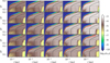 |
Fig. D.2 Same as Fig. D.1, but for CO. The dashed line indicates the τCO=1 line. |
| In the text | |
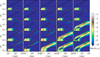 |
Fig. D.3 Same as Fig. D.1, but for C2H2. The dashed line indicates the |
| In the text | |
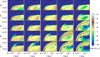 |
Fig. D.4 Same as Fig. D.3, but zoomed-in. |
| In the text | |
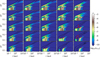 |
Fig. D.5 Same as Fig. D.1, but for CO2. The dashed line indicates the τCO2=1 line. |
| In the text | |
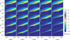 |
Fig. D.6 Same as Fig. D.1, but for OH. The dashed line indicates the τOH=1 line. |
| In the text | |
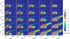 |
Fig. D.7 Same as Fig. D.1, but for HCN. The dashed line indicates the τHCN=1 line. |
| In the text | |
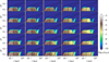 |
Fig. D.8 Same as Fig. D.1, but for NH3. The dashed line indicates the τNH3=1 line. |
| In the text | |
|
Fig. D.9 Same as Fig. D.1, but for Ne+. The dashed line indicates the τ[NeII]=1 line. Note the different axes limits. |
| In the text | |
|
Fig. E.1 Same as Fig. 7, but including models with C/O>1. The colors of the points correspond to the C/O ratios (see Fig. 6). The models with C/O>1 are at the bottom-left corner of each panel. |
| In the text | |
|
Fig. E.2 Same as Fig. 7, but for observations of disks around VLMSs, and the wavelength intervals are adapted for these sources. The spectra and detections are taken from Arabhavi et al. (2025a), Arabhavi et al. (2025b), and Xie et al. (2023). |
| In the text | |
Current usage metrics show cumulative count of Article Views (full-text article views including HTML views, PDF and ePub downloads, according to the available data) and Abstracts Views on Vision4Press platform.
Data correspond to usage on the plateform after 2015. The current usage metrics is available 48-96 hours after online publication and is updated daily on week days.
Initial download of the metrics may take a while.