| Issue |
A&A
Volume 708, April 2026
|
|
|---|---|---|
| Article Number | A163 | |
| Number of page(s) | 12 | |
| Section | Extragalactic astronomy | |
| DOI | https://doi.org/10.1051/0004-6361/202556400 | |
| Published online | 03 April 2026 | |
Large-amplitude modulations and hours-timescale variability in the early X-ray light curve of a tidal disruption flare
1
Max-Planck-Institut für Extraterrestrische Physik, Giessenbachstrasse 1, 85748, Garching, Germany
2
Università degli Studi di Milano, Via Giovanni Celoria 16, 20134, Milano, Italy
3
INFN, Sezione di Milano-Bicocca, Piazza della Scienza 3, I-20126, Milano, Italy
4
Nicolaus Copernicus Astronomical Center, Polish Academy of Sciences, ul. Bartycka 18, 00-716, Warszawa, Poland
5
International Centre for Radio Astronomy Research – Curtin University, GPO Box U1987, Perth, WA, 6845, Australia
6
Leibniz-Institut für Astrophysik Potsdam, An der Sternwarte 16, 14482, Potsdam, Germany
★ Corresponding author: This email address is being protected from spambots. You need JavaScript enabled to view it.
Received:
14
July
2025
Accepted:
11
February
2026
Abstract
We present new X-ray, optical, and UV observations of the tidal disruption event candidate eRASSt J234402.9−352640 (hereafter J2344). Between 50 and 60 days after peak optical brightness, J2344 exhibited large-amplitude modulations in its 0.2−2 keV emission, when the flux repeatedly dimed and re-brightened by a factor of ∼6 over a ∼3-day timescale. These modulations exhibited harder-when-brighter behaviour but were not detected in high-cadence observations obtained 60−70 days and 170−200 days after peak optical brightness, when the system instead exhibited stochastic X-ray variability over timescales of hours. We discuss the different physical mechanisms responsible for such exotic X-ray variability and explore the possibility that the modulations in J2344 were caused by the Lense-Thirring precession of the inner accretion flow around the disrupting black hole.
Key words: accretion / accretion disks / galaxies: active / X-rays: individuals: eRASSt J234402.9–352640
© The Authors 2026
 Open Access article, published by EDP Sciences, under the terms of the Creative Commons Attribution License (https://creativecommons.org/licenses/by/4.0), which permits unrestricted use, distribution, and reproduction in any medium, provided the original work is properly cited.
This article is published in open access under the Subscribe to Open model.
Open access funding provided by Max Planck Society.
1. Introduction
Stellar tidal disruption events (TDEs; Rees 1988) offer a unique way to study accretion onto supermassive black holes (SMBHs) and probe their mass, MBH, and spin, a. In recent years, various efforts have explored constraining these properties from the emission produced by TDE flares. These include (i) fitting X-ray spectra using models of the TDE disc emission, i.e. non-stationary relativistic models of thin accretion discs (e.g. Mummery & Balbus 2020) and stationary slim accretion discs (Wen et al. 2020, 2022), (ii) fitting the multi-band optical-UV photometric light curves of TDEs using models that assume the optical emission is produced by stream-stream collisions (Ryu et al. 2020) or reprocessed accretion models (Guillochon et al. 2018; Mockler et al. 2019), and (iii) scaling relationships between the late-time optical luminosities of TDEs and black hole masses (Mummery et al. 2023).
This paper reports additional X-ray and photometric observations of the TDE candidate eRASSt J234402.9−352640 (hereafter J2344; Homan et al. 2023), which was discovered by the extended ROentgen Survey with an Imaging Telescope Array (eROSITA; Predehl et al. 2021) on board the Spektrum-Roentgen-Gamma (SRG) observatory (Sunyaev et al. 2021) as an ultra-soft flare from a galaxy at z = 0.1. The host galaxy contains a low-luminosity active galactic nucleus (Homan et al. 2023) with a central black hole mass of log(MBH/M⊙) = 7.2 ± 0.4 (Appendix A). In Sect. 2 we present an overview of the multi-wavelength follow-up campaign of J2344, before analysing the X-ray evolution in Sect. 3. We then discuss the possible physical mechanisms driving the X-ray variability in Sect. 4, and summarise our work in Sect. 5. We adopted a flat ΛCDM cosmology throughout this work, with H0 = 67.7 km s−1 Mpc−1 and Ωm = 0.309 (Planck Collaboration XIII 2016); z = 0.1 therefore corresponds to a luminosity distance of 475 Mpc. All magnitudes are reported in the AB system, unless otherwise stated, and have been corrected for Galactic extinction using AV = 0.0386 mag (Schlafly & Finkbeiner 2011), RV = 3.1, and a Cardelli et al. (1989) extinction curve. All dates and times are reported in universal time (UT), and we define the time of peak optical brightness, tpeak, to be MJD = 59170.
2. Observations
A multi-wavelength follow-up campaign of J2344 was initiated after its detection in the second eROSITA all-sky survey (eRASS2). Details regarding the observations and their associated data reduction are presented in Appendix B. The extensive set of X-ray observations provided by eROSITA, Swift/X-ray Telescope (XRT), XMM/EPIC-pn, the Neutron Star Interior Composition Explorer (NICER)/X-ray Timing Instrument (XTI), and Chandra/Advanced CCD Imaging Spectrometer (ACIS) makes J2344 one of the best monitored non-jetted TDE candidates to date over the 0.2−10 keV range. The multi-wavelength evolution of J2344 is plotted in Fig. 1, and a summary of the X-ray flux evolution and optical/UV photometry is presented in Tables C.1 and C.2, respectively.
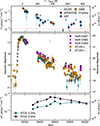 |
Fig. 1. Multi-wavelength light curve evolution of J2344, with the unabsorbed 0.2−2 keV fluxes (top panel) and the optical and UV fluxes (middle). Triangular data points denote 3σ upper limits on the flux. The horizontal dashed red line in the X-ray light curve panel denotes the 3σ upper limit on the 0.2−2 keV flux inferred from the non-detection of J2344 in eRASS1 (Homan et al. 2023), approximately 200 days before optical peak. The radio evolution (bottom panel) is well described by an expanding synchrotron-emitting region from a single ejection of material, consistent with an outflow launched by a non-relativistic TDE (Goodwin et al. 2024). |
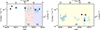 |
Fig. 2. Zoomed-in view of the X-ray evolution during the high-cadence NICER observations. The two panels have the same y-axis and cover the same amount of time on the x-axis. The different shaded backgrounds denote windows W1, W2, and W3 for the NICER observations (Sect. 3.1.3), taken 50−60 days, 60−70 days, and 165−210 days after optical peak. |
3. X-ray evolution
3.1. Spectral fitting
The extracted X-ray spectra were fitted using the Bayesian X-ray Analysis (BXA) software (Buchner et al. 2014), which connects the nested sampling algorithm UltraNest1 (Buchner 2021) with an X-ray spectral fitting environment. The eROSITA, XMM/EPIC-pn (Strüder et al. 2001), Chandra/ACIS, and Swift/XRT spectra were fitted using CIAO/Sherpa (Fruscione et al. 2006), with their background spectra jointly modelled using a principle-component-analysis-based approach (Simmonds et al. 2018). The NICER/XTI spectra were fitted using XSPEC, with the background contribution to the spectra modelled using the HEASOFT tool SCORPEON2. The eROSITA, XMM/pn, Swift/XRT, Chandra/ACIS, and NICER/XTI spectra were fitted in the 0.2−8 keV, 0.2−10 keV, 0.5−7 keV, 0.3−10 keV, and 0.22−15 keV energy bands, respectively. All spectra were fitted using the C-statistic (Cash 1976) and were unbinned for fitting. Lastly, each fitted spectral model was absorbed by a total (HI + H2) Galactic hydrogen column density of 1.2 × 1020 cm−2 (Willingale et al. 2013; Homan et al. 2023), with abundances adopted from Wilms et al. (2000) and cross-sections from Verner et al. (1996).
Before exploring more complex spectral models, we fitted a simple power-law model (tbabs*powerlaw, with NH = 1.2 × 1020 cm−2) to each X-ray spectrum to gain a first-order understanding of the X-ray spectral evolution. Over the ∼770-day X-ray monitoring campaign, the X-ray spectra remained ultra-soft (photon indices ≳4; Fig. 3) and without a clear active-galactic-nucleus-like power-law component produced by inverse-Compton-scattered disc photons (e.g. Nandra & Pounds 1994). The X-ray emission at late times is also in excess of the 3σ pre-flare upper limit on the 0.2−2 keV flux of 1.1 × 10⁻¹³ erg cm−2 s−1 (Homan et al. 2023) provided by the non-detection of J2344 in eRASS1, suggesting that this emission is associated with the recent enhanced accretion episode.
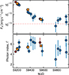 |
Fig. 3. Joint evolution of the observed 0.2−2 keV flux (top panel) and the photon index (bottom panel) over time. The dashed red line marks the 3σ flux upper limit inferred from the non-detection in eRASS1. The X-ray spectrum remains ultra-soft (Γ ≳ 4) over the ∼760 days of X-ray monitoring (∼800 days after optical peak; Homan et al. 2023). |
3.1.1. eROSITA and XMM spectra
The three eROSITA and three XMM spectra, obtained between ∼20 days and ∼400 days after the peak optical brightness, provide the strongest constraints on the X-ray spectral properties of J2344. We fitted eight different models (Table D.1) to each spectrum, with the choice of models guided by previous models used in the literature to fit the ultra-soft spectra of TDEs, as well as the model fitting performed in Homan et al. (2023). For each fitted model, we computed the Akaike information criterion,  , where k is the number of free parameters in the model and
  is the maximum likelihood of the fit. The best fitting model to each spectrum is the one with the lowest AIC. The best fitting models to the eROSITA and XMM spectra are presented in Figs. D.2 and D.3, respectively, and the spectral fit results are presented in Table E.1.
The preferred model fit for the eRASS2 spectrum is the dual blackbody (zbbody+zbbody) model, with  eV and
  eV. For the fainter eRASS3 and eRASS4 spectra, a power-law model (zpowerlaw) is preferred, with
  and
and  , respectively. For XMM1 and XMM3, the preferred fit is again the double blackbody model, with
  eV and
  eV in XMM1, and
  eV and
  eV in XMM3. However, the preferred fitted model for the XMM2 spectrum is an absorbed power law (ztbabs*zpowerlaw), with
 ![Mathematical equation: $ \log [N_{\mathrm{H}}/\mathrm{cm}^2] = 19.97^{+0.08}_{-0.11} $](/articles/aa/full_html/2026/04/aa56400-25/aa56400-25-eq11.gif) and
and  , with the dual blackbody model under-predicting the model flux in the 1−2 keV range (Fig. D.3).
3.1.2. Chandra and Swift spectra
Since the Swift/XRT and Chandra spectra were fitted over the 0.3−10 keV and 0.5−7 keV ranges, respectively, and possess lower signal/noise values, these observations place weaker constraints on the spectral properties of the ultra-soft emission in J2344 in comparison to the eROSITA and XMM spectra. Therefore, we focused on using these spectra to measure 0.2−2 keV fluxes and complete J2344’s X-ray light curve, leaving spectral parameter estimation to the higher signal/noise spectra (Sect. 3.1.1). To do this, we fitted each spectrum with a dual blackbody model where kT1 and kT2 were constrained to between 35 eV and 55 eV, and 100 eV and 140 eV, respectively, whilst the normalisations of each component were left free to vary. For Swift/XRT epochs where J2344 was not significantly detected above the background, the 0.2−2 keV flux upper limits were generated from the 0.3−2 keV count rate upper limits (Appendix B.2) using webPIMMs3; we adopted the spectral model inferred from our fit to the first XMM spectrum to convert from count rates to fluxes.
3.1.3. NICER spectra
Each NICER spectrum generated from a good time interval (GTI) with exposure above 100 s (Appendix B.4) was fitted with the same constrained phenomenological dual blackbody model used for the Swift/XRT and Chandra spectra (Sect. 3.1.2). Homan et al. (2023) also fitted a dual blackbody model to the stacked NICER spectra over the 0.3−2 keV range using the first ∼6 days of observations, finding kT1 = 59 ± 1 eV and kT2 = 105 ± 3 eV; they also found that single blackbody and single power-law models provided poor fits to these spectra.
To aid in describing the spectral evolution during the NICER observations, we refer to NICER observations taken 50−60 days, 60−70 days, and 165−210 days after optical peak as windows 1, 2, and 3, respectively (i.e. W1, W2, and W3; Fig. 1). In W1, the 0.2−2 keV flux undergoes a series of large-amplitude modulations during which the flux drops by a factor of ∼6 over 1.5 days before re-brightening over the following 1.5 days, with this cycle repeating two more times in W1 (a more detailed timing analysis is presented in Sect. 3.2). During W1, the emission in the 0.2−2 keV band is dominated by the softer blackbody, the spectrum is harder when brighter (Figs. 4 and D.1), and the normalisation of the two blackbody components increases when the system is in the brighter stage of a modulation. In W2 and W3, the modulations are not observed and the 0.2−2 keV flux evolution is more stochastic, with the emission dominated by the softer blackbody. We note that W2 immediately follows W1, implying that the modulations disappeared abruptly.
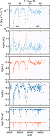 |
Fig. 4. Top panel: Evolution of the 0.2−2 keV flux, FX, over time during the high-cadence NICER observations at early times (∼50 days after optical peak). Second panel: spectral hardness estimated as log[A1/A2], with A1 and A2 the normalisation of the softer and harder blackbody components, respectively. Since smaller log[A1/A2] values correspond to harder spectra, J2344 exhibits a harder-when-brighter behaviour. Third and fourth panels: log A1 and log A2 in units of L39/[D10(1 + z)]2, with L39 the luminosity in 1039 erg s−1 and D10 the distance to the source in units of 10 kpc. Bottom panel: Evolution of the blackbody temperatures for each model component. The kT1 (orange) and kT2 (blue) were constrained to the 35−55 eV and 100−140 eV ranges during fitting. |
3.2. X-ray light curve evolution
3.2.1. Long-term evolution
We fitted the 0.2−2 keV light curve with an exponential decline model, FX(t) = Fpeakexp[−(t−tpeak)/τ], and a power-law model, FX(t) = Fpeak(1 + (t − tpeak)/t0)−p. Here, the NICER data taken before MJD 59240 were excluded when the X-ray light curve exhibited modulations. In addition, we constrained tpeak to 59165 to 59175 for both models (based on the observed optical peak; Fig. 1), and fixed p to 5/3 for the power-law model. The inferred Fpeak is  erg cm−2 s−1 for the power-law model with
  days, whilst
  erg cm−2 s−1 and
  days for the exponential decay. These fitted models are shown in Fig. 5. Neither model fits the data particularly well: the exponential model under-predicts the peak flux and the late-time X-ray emission, while the power-law model over-predicts the flux at ∼200 − 600 days after optical peak but fits the X-ray fluxes > 600 days after optical peak reasonably well.
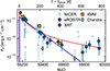 |
Fig. 5. Power-law decay (red) and exponential decay (blue) models fitted to the 0.2−2 keV X-ray light curve of J2344 (excluding the early-time NICER data that exhibit modulations). The late-time flattening in the X-ray fluxes is better fitted by the power-law model here. |
3.2.2. Early-time modulations and hours-timescale X-ray variability
The joint set of X-ray observations of J2344 reveals large-amplitude modulations in its 0.2−2 keV emission (Fig. 1), with three clear modulations detected during the initial high-cadence NICER monitoring observations performed in W1 (∼50 − 60 days after tpeak). After the re-brightening observed in the last full modulation (∼60 days after optical peak), the X-ray flux initially starts to decrease, similarly to the start of the other three modulations, but then begins exhibiting stochastic variations with a median flux of FX, unabsorbed = 8.9 × 10⁻¹² erg cm−2 s−1, fainter than the peak flux observed during one of the modulations (FX, unabsorbed ≈ 1.3 × 10⁻¹¹ erg cm−2 s−1). Modulations were also not detected in the post-sunblock NICER monitoring window at ∼170 − 200 days after tpeak, with the 0.2−2 keV source flux in these late-time observations almost an order of magnitude brighter than the sensitivity limits of NICER (i.e. we should have been able to detect similar-amplitude modulations in this monitoring window if they were still present). J2344 also exhibits hours-timescale variability during W2 and W3, where the X-ray flux is observed to change by up to a factor of ∼2 over ∼4-hour timescales4 (Fig. 6), similar to the hours-timescale X-ray variability reported in Yao et al. (2024).
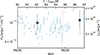 |
Fig. 6. Zoom in on the hours-timescale stochastic X-ray variability during W2, after the shut-off of the large amplitude modulations. The two dashed red lines are separated by ∼3 hours, and the X-ray flux varies by a factor of 2 between these observations. |
The early-time X-ray light curve also shows tentative evidence of periodic behavior. The Lomb-Scargle periodogram (LSP; Lomb 1976; Scargle 1982) computed from the pre-sunblock light curve between MJD 59215 and 59240 reveals a clear peak at  d, which we consider statistically significant at > 4σ (Figure 7, see also Appendix D.2 for a detailed discussion). This periodicity is driven by the repeated modulations in W1 described above, since no significant peak is observed in the LSP when computed from NICER data taken only in W2. The phase-folded light curve in Fig. 8 highlights that the X-ray spectrum softens in each modulation cycle as the flux drops; although the peak flux in each modulation is roughly constant, the shape of the dip is asymmetric, with the dimming faster than the brightening in each modulation. However, we caution that the major caveat to this detection of periodicity is that we have ultimately only observed three putative cycles, and pure red-noise processes can routinely mimic 3−4 cycle sinusoid-like periodicities (Vaughan et al. 2016). Robust detections of quasi-periodicity in accreting active galactic nuclei in cases where the light curves exhibit a low number of cycles – that is, fully ruling out that the signal is red noise – have not been convincingly achieved yet.
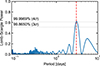 |
Fig. 7. LSP computed from the 0.2−2 keV light curve between MJD 59215 and 59240. The dashed red line marks the period |

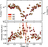 |
Fig. 8. Folded 0.2−2 keV flux light curve (top panel) and hardness (bottom panel) of the NICER data from W1. In each modulation, the X-ray spectrum softens (higher log[A1/A2]) when the flux drops. The data points are coloured based upon which modulation they are associated with – M1, M2, or M3 – with M1 starting at MJD = 59220.3, and the light curves are folded with a periodicity of 3.05 days (this is consistent with the periodicity estimate of |

4. Discussion
In the following, we explore possible physical origins of the large-amplitude X-ray modulations observed in J2344. While we currently favour a precession-related scenario (see Sect. 4.1), we also consider alternative explanations and outline the reasons they are less likely in Sect. 4.2.
4.1. Precession of the inner accretion flow?
As tidally disrupted stars can approach the black hole isotropically (Stone et al. 2020), a large fraction of TDEs will have misaligned stellar orbits and black hole equatorial planes. If the stellar debris circularises promptly around the black hole, then the newly formed accretion disc may be misaligned with the black hole’s equatorial plane. However, since spinning black holes will exert a frame-dragging effect on the nascent accretion disc, a torque acts to align the angular momentum of the accretion disc with the black hole spin. For the thick, compact accretion discs predicted to form in TDEs, the disc may initially precess as a solid body (Stone & Loeb 2012; Shen & Matzner 2014; Franchini et al. 2016). As the disc precesses, a distant observer would periodically glimpse into the inner, hotter annuli of the disc, with the disc appearing brighter and harder when this occurs (Stone et al. 2019). The precession therefore leads to periodic modulations in the soft X-ray emission from the transient at early times, as observed recently in AT 2020ocn (Pasham et al. 2024); this is also consistent with the X-ray light curve for J2344. Following Franchini et al. (2016) to estimate the precession period, and assuming the disruption of a Sun-like star by a black hole with log[MBH/M⊙] = 7.2, a spin of a = 0.6 would yield a precession timescale consistent with the observed 3-day timescale of modulations (Fig. 9). However, if the currently unknown mass of the disrupted star were lower (higher), then a lower (higher) black hole spin would be needed to produce a precession period consistent with the observed periodicity (M★/M⊙ = 0.1 would need a = 0.15, whilst M★/M⊙ = 3 would need a = 0.95; Fig. 9). We note that the precession timescale also strongly depends on the disc surface density profile: a disc that is denser in the outer parts would precess on a much longer timescale. In the above, we assumed the surface density to be a decreasing function of radius, following the stabilisation of the radiation-pressure-dominated disc against the Lightman & Eardley (1974) instability, but a strong magnetic pressure can also stabilise the disc against the thermal instability and cause the surface density of the disc to decrease with radius (Kaur et al. 2023).
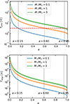 |
Fig. 9. Precession (top panel) and alignment (bottom panel) timescales for a global precessing disc, plotted against black hole spin (a) for three stars of different masses being disrupted, assuming log[MBH/M⊙] = 7.2 (Appendix A). The shaded regions enclose the uncertainty on each timescale due to the 1σ uncertainty on log[MBH/M⊙]. These timescales were computed with H/R = 0.1 and α = 0.1, following Franchini et al. (2016). The dashed red line in the top panel denotes the observed 3-day modulation timescale observed in J2344, and the vertical grey lines denote the spin values that make Tprec consistent with 3 days (e.g. a ∼ 0.6 for a Sun-like star), highlighting that spin constraints derived from this approach are sensitive to the assumed mass of the disrupted star. |
At late times post-disruption, the X-ray modulations are predicted to ‘turn off’ because the solid body precession cannot be maintained, either due to the disc thinning over time as the accretion rate decreases (Stone & Loeb 2012; Shen & Matzner 2014) or if the disc eventually becomes aligned with the black hole spin (see Franchini et al. 2016 for a discussion of the relative importance of each effect in halting the solid body precession). Assuming an aspect ratio for the TDE disc of H/R = 1 and disc viscosity parameter α = 0.1, Franchini et al. (2016) predict an alignment timescale of ∼40 days, which would be long enough for us to have observed the modulations in J2344 at 50−60 days after optical peak. However, the sudden turn-off of the X-ray modulations observed in J2344 between W1 and W2 (Fig. 2), which implies a sudden halting of the global disc precession, is different from the more gradual alignment behaviour predicted in Franchini et al. (2016).
An alternative to the global disc precession scenario is that the X-ray modulations were caused by the precession of an inner disc after the tearing of the initial TDE disc into discrete rings (Nixon et al. 2012). For a disc broken at radius Rbreak ≈ 16Rg(a/0.5)2/3(α/0.1)−2/3((H/R)/0.1)−2/3 (Nixon et al. 2012), the inner disc material is expected to precess on the local Lense-Thirring timescale, Tprec ≈ 4(a/0.5)(α/0.1)−2(H/R/0.1)−2(MBH/107.2 M⊙) days (Nixon et al. 2012; Raj & Nixon 2021), and could therefore be capable of producing the 3-day modulation timescale seen in J2344. As the inner ring spreads outwards over time, collisions may occur between neighbouring rings, leading to an increased accretion rate onto the black hole and a period of higher luminosity (Raj & Nixon 2021). This would quench the modulations, similarly to what was observed in J2344 between W1 and W2, and would be an advantage of using the disc tearing model to explain the modulations in J2344 over the global precession model. We note, though, that the shape of the flares in the accretion rate from disc tearing differs from the dip-like modulations observed in J2344 (see Fig. 3 in Raj & Nixon 2021).
4.2. Alternate origins
The differential precession of the stellar debris streams and their violent self-intersection has been proposed to drive the early-time flaring in TDEs (Andalman et al. 2021), with periodic self-intersections driving periodic modulations of the accretion rate. However, they are predicted to only be present at early times during the disc formation process and therefore likely do not produce the modulations observed ∼50−60 days after the optical peak in J2344, since we expect the disc to already have been established by the time of the first eROSITA detection.
The harder-when-brighter behaviour of the system rules out the modulations being produced by lensing by a compact orbiting body, as has been considered to explain repeated X-ray outbursts in galactic centres (Ingram et al. 2021), and also rules out a variable neutral absorber. It is possible that this X-ray variability is linked to changing ionised absorption, but one would still need a mechanism to explain the repeated modulations every ∼3 days. A combination of a precessing disc and repeatedly viewing along a given angle of a disc wind, as seen in X-ray binaries (e.g. Kosec et al. 2023), may also explain the observed modulations.
Sinusoidal-like modulations of the emission from a system involving a SMBH binary have been predicted. However, the system would be extremely close to merging if the modulation timescale of the X-rays in J2344 is associated with the SMBH binary’s orbital period, and it would be highly unlikely to have observed such a system at z = 0.1. Alternate variants of the binary model, such as the modulations being produced by collisions between an orbiting body and an accretion disc, are disfavoured due to the absence of such flares during NICER windows W2 and W3. Furthermore, such variants can require a large amount of fine-tuning to make the observed recurrence timescale of the outburst match the outburst duration.
Lastly, Baldini et al. (2026) report the detection of quasi-periodic eruptions from J2344 in Einstein Probe and XMM–Newton observations obtained more than four years after the X-ray peak. These short-duration (∼2 h) thermal flares recurred on a timescale of ∼12 h and persisted for at least nine months; they interpreted them as arising from repeated interactions between a third body and the accretion disc formed during the TDE. Their markedly different phenomenology and characteristic timescales, relative to the modulations reported here, suggest that the two phenomena are physically distinct.
5. Summary
The key observational signatures of J2344 reported in this work are:
-
An ultra-soft (photon indices ≳4), large-amplitude flare (≳150× brightening in the 0.2−2 keV band) from a low-luminosity active galactic nucleus, reaching a peak observed 0.2−2 keV luminosity of
 erg s−1. The X-ray emission remains ultra-soft over the course of the ∼800 day follow-up campaign.
 -
J2344 also shows transient optical and UV emission, with its optical light curve characterised by a fast rise to peak (∼50 days), followed by a decline period over at least the following ∼800 days. Along with ASASSN-14li, J2344 is one of the few TDE candidates that show a near contemporaneous optical and X-ray brightening, as well as a well-sampled, relatively smooth X-ray decline over months-long timescales.
-
Between 50 and 60 days after optical peak, the high-cadence NICER observations reveal large-amplitude modulations of the ultra-soft X-ray emission, where the X-ray flux repeatedly dims and re-brightens by a factor of ∼6 over a ∼3.1-day timescale, and the X-ray emission becomes harder when brighter. These modulations are not detected in NICER observations 60−70 days and 170−200 days after the optical peak.
Although the physical mechanism producing these X-ray modulations is still unclear, we currently favour a precession-related origin (Sect. 4.1) in order to explain the tentative 3-day periodicity in the early X-ray light curve.
Acknowledgments
We thank the anonymous referee for the insightful comments that helped improving the paper. AM is grateful to the generosity of Curtin University for hosting his visit, where parts of this work were completed. AM also thanks the Yukawa Institute for Theoretical Physics at Kyoto University, where discussions held during the YITP International Molecule-type Workshop YITP-T-19-07 on “Tidal Disruption Events: General Relativistic Transients” were useful for completing this work. AM thanks the Chandra, NICER, Swift and XMM teams for approving the ToO requests. AM acknowledges support by DLR under the grant 50 QR 2110 (XMM_NuTra, PI: Z. Liu). This work was supported by the Australian government through the Australian Research Council’s Discovery Projects funding scheme (DP200102471). AGM acknowledges support from Narodowe Centrum Nauki (NCN) grant 2018/31/G/ST9/03224, and partial support from NCN grant 2019/35/B/ST9/03944. This work is based on data from eROSITA, the soft X-ray instrument aboard SRG, a joint Russian-German science mission supported by the Russian Space Agency (Roskosmos), in the interests of the Russian Academy of Sciences represented by its Space Research Institute (IKI), and the Deutsches Zentrum für Luft- und Raumfahrt (DLR). The SRG spacecraft was built by Lavochkin Association (NPOL) and its subcontractors, and is operated by NPOL with support from the Max Planck Institute for Extraterrestrial Physics (MPE). The development and construction of the eROSITA X-ray instrument was led by MPE, with contributions from the Dr. Karl Remeis Observatory Bamberg & ECAP (FAU Erlangen-Nuernberg), the University of Hamburg Observatory, the Leibniz Institute for Astrophysics Potsdam (AIP), and the Institute for Astronomy and Astrophysics of the University of Tübingen, with the support of DLR and the Max Planck Society. The Argelander Institute for Astronomy of the University of Bonn and the Ludwig Maximilians Universität Munich also participated in the science preparation for eROSITA.
References
- Andalman, Z. L., Liska, M. T. P., Tchekhovskoy, A., Coughlin, E. R., & Stone, N. 2021, MNRAS, 510, 1627 [Google Scholar]
- Baldini, P., Rau, A., Merloni, A., et al. 2026, A&A, 706, L15 [NASA ADS] [CrossRef] [EDP Sciences] [Google Scholar]
- Brunner, H., Liu, T., Lamer, G., et al. 2022, A&A, 661, A1 [NASA ADS] [CrossRef] [EDP Sciences] [Google Scholar]
- Buchner, J. 2021, J. Open Source Softw., 6, 3001 [CrossRef] [Google Scholar]
- Buchner, J., Georgakakis, A., Nandra, K., et al. 2014, A&A, 564, A125 [NASA ADS] [CrossRef] [EDP Sciences] [Google Scholar]
- Burke, C. J., Shen, Y., Blaes, O., et al. 2021, Science, 373, 789 [NASA ADS] [CrossRef] [Google Scholar]
- Burrows, D. N., Hill, J. E., Nousek, J. A., et al. 2005, Space Sci. Rev., 120, 165 [Google Scholar]
- Cardelli, J. A., Clayton, G. C., & Mathis, J. S. 1989, ApJ, 345, 245 [Google Scholar]
- Cash, W. 1976, A&A, 52, 307 [NASA ADS] [Google Scholar]
- Emmanoulopoulos, D., McHardy, I. M., & Papadakis, I. E. 2013, MNRAS, 433, 907 [NASA ADS] [CrossRef] [Google Scholar]
- Evans, P. A., Beardmore, A. P., Page, K. L., et al. 2007, A&A, 469, 379 [NASA ADS] [CrossRef] [EDP Sciences] [Google Scholar]
- Evans, P. A., Beardmore, A. P., Page, K. L., et al. 2009, MNRAS, 397, 1177 [Google Scholar]
- Foreman-Mackey, D., Agol, E., Ambikasaran, S., & Angus, R. 2017, AJ, 154, 220 [Google Scholar]
- Franchini, A., Lodato, G., & Facchini, S. 2016, MNRAS, 455, 1946 [NASA ADS] [CrossRef] [Google Scholar]
- Fruscione, A., McDowell, J. C., Allen, G. E., et al. 2006, Proc. SPIE, 6270, 62701V [Google Scholar]
- Garmire, G. P., Bautz, M. W., Ford, P. G., Nousek, J. A., & Ricker, G. R. 2003, Proc. SPIE, 4851, 28 [NASA ADS] [CrossRef] [Google Scholar]
- Gendreau, K. C., Arzoumanian, Z., Adkins, P. W., et al. 2016, Proc. SPIE, 9905, 99051H [NASA ADS] [CrossRef] [Google Scholar]
- Goodwin, A. J., Anderson, G. E., Miller-Jones, J. C. A., et al. 2024, MNRAS, 528, 7123 [Google Scholar]
- Guillochon, J., Nicholl, M., Villar, V. A., et al. 2018, ApJS, 236, 6 [NASA ADS] [CrossRef] [Google Scholar]
- Gültekin, K., Richstone, D. O., Gebhardt, K., et al. 2009, ApJ, 698, 198 [Google Scholar]
- Hammerstein, E., van Velzen, S., Gezari, S., et al. 2023, ApJ, 942, 9 [NASA ADS] [CrossRef] [Google Scholar]
- Homan, D., Krumpe, M., Markowitz, A., et al. 2023, A&A, 672, A167 [NASA ADS] [CrossRef] [EDP Sciences] [Google Scholar]
- Ingram, A., Motta, S. E., Aigrain, S., & Karastergiou, A. 2021, MNRAS, 503, 1703 [NASA ADS] [CrossRef] [Google Scholar]
- Kaspi, S., Maoz, D., Netzer, H., et al. 2005, ApJ, 629, 61 [Google Scholar]
- Kaur, K., Stone, N. C., & Gilbaum, S. 2023, MNRAS, 524, 1269 [NASA ADS] [CrossRef] [Google Scholar]
- Kiehlmann, S. 2023, Astrophysics Source Code Library [record ascl:2310.002] [Google Scholar]
- Kochanek, C. S., Shappee, B. J., Stanek, K. Z., et al. 2017, PASP, 129, 104502 [Google Scholar]
- Kosec, P., Kara, E., Fabian, A. C., et al. 2023, Nat. Astron., 7, 715 [Google Scholar]
- Le, H. A. N., Xue, Y., Lin, X., & Wang, Y. 2023, ApJ, 945, 59 [NASA ADS] [CrossRef] [Google Scholar]
- Lightman, A. P., & Eardley, D. M. 1974, ApJ, 187, L1 [Google Scholar]
- Lomb, N. R. 1976, Ap&SS, 39, 447 [Google Scholar]
- Mockler, B., Guillochon, J., & Ramirez-Ruiz, E. 2019, ApJ, 872, 151 [Google Scholar]
- Mummery, A., & Balbus, S. A. 2020, MNRAS, 492, 5655 [NASA ADS] [CrossRef] [Google Scholar]
- Mummery, A., van Velzen, S., Nathan, E., et al. 2023, MNRAS, 527, 2452 [NASA ADS] [CrossRef] [Google Scholar]
- Nandra, K., & Pounds, K. A. 1994, MNRAS, 268, 405 [Google Scholar]
- Nicholl, M., Wevers, T., Oates, S. R., et al. 2020, MNRAS, 499, 482 [NASA ADS] [CrossRef] [Google Scholar]
- Nixon, C., King, A., Price, D., & Frank, J. 2012, ApJ, 757, L24 [NASA ADS] [CrossRef] [Google Scholar]
- Pasham, D. R., Zajaček, M., Nixon, C. J., et al. 2024, Nature, 630, 325 [NASA ADS] [CrossRef] [Google Scholar]
- Planck Collaboration XIII. 2016, A&A, 594, A13 [NASA ADS] [CrossRef] [EDP Sciences] [Google Scholar]
- Predehl, P., Andritschke, R., Arefiev, V., et al. 2021, A&A, 647, A1 [EDP Sciences] [Google Scholar]
- Raj, A., & Nixon, C. J. 2021, ApJ, 909, 82 [NASA ADS] [CrossRef] [Google Scholar]
- Rees, M. J. 1988, Nature, 333, 523 [Google Scholar]
- Roming, P. W. A., Kennedy, T. E., Mason, K. O., et al. 2005, Space Sci. Rev., 120, 95 [Google Scholar]
- Ryu, T., Krolik, J., & Piran, T. 2020, ApJ, 904, 73 [NASA ADS] [CrossRef] [Google Scholar]
- Salviander, S., Shields, G. A., Gebhardt, K., & Bonning, E. W. 2007, ApJ, 662, 131 [NASA ADS] [CrossRef] [Google Scholar]
- Scargle, J. D. 1982, ApJ, 263, 835 [Google Scholar]
- Schlafly, E. F., & Finkbeiner, D. P. 2011, ApJ, 737, 103 [Google Scholar]
- Shen, Y., & Kelly, B. C. 2010, ApJ, 713, 41 [NASA ADS] [CrossRef] [Google Scholar]
- Shen, R.-F., & Matzner, C. D. 2014, ApJ, 784, 87 [NASA ADS] [CrossRef] [Google Scholar]
- Shingles, L., Smith, K. W., Young, D. R., et al. 2021, TNSAN, 7, 1 [NASA ADS] [Google Scholar]
- Simmonds, C., Buchner, J., Salvato, M., Hsu, L.-T., & Bauer, F. E. 2018, A&A, 618, A66 [EDP Sciences] [Google Scholar]
- Smith, K. W., Smartt, S. J., Young, D. R., et al. 2020, PASP, 132, 085002 [Google Scholar]
- Stone, N., & Loeb, A. 2012, Phys. Rev. Lett., 108, 061302 [NASA ADS] [CrossRef] [Google Scholar]
- Stone, N. C., Kesden, M., Cheng, R. M., & van Velzen, S. 2019, Gen. Relat. Grav., 51, 30 [CrossRef] [Google Scholar]
- Stone, N. C., Vasiliev, E., Kesden, M., et al. 2020, Space Sci. Rev., 216, 35 [NASA ADS] [CrossRef] [Google Scholar]
- Strüder, L., Briel, U., Dennerl, K., et al. 2001, A&A, 365, L18 [Google Scholar]
- Sunyaev, R., Arefiev, V., Babyshkin, V., et al. 2021, A&A, 656, A132 [NASA ADS] [CrossRef] [EDP Sciences] [Google Scholar]
- Timmer, J., & Koenig, M. 1995, A&A, 300, 707 [NASA ADS] [Google Scholar]
- Tonry, J. L., Denneau, L., Heinze, A. N., et al. 2018, PASP, 130, 064505 [Google Scholar]
- Turner, M. J. L., Abbey, A., Arnaud, M., et al. 2001, A&A, 365, L27 [CrossRef] [EDP Sciences] [Google Scholar]
- van Velzen, S. 2018, ApJ, 852, 72 [NASA ADS] [CrossRef] [Google Scholar]
- VanderPlas, J. T. 2018, ApJS, 236, 16 [Google Scholar]
- Vaughan, S., Uttley, P., Markowitz, A. G., et al. 2016, MNRAS, 461, 3145 [Google Scholar]
- Verner, D. A., Ferland, G. J., Korista, K. T., & Yakovlev, D. G. 1996, ApJ, 465, 487 [Google Scholar]
- Wen, S., Jonker, P. G., Stone, N. C., Zabludoff, A. I., & Psaltis, D. 2020, ApJ, 897, 80 [NASA ADS] [CrossRef] [Google Scholar]
- Wen, S., Jonker, P. G., Stone, N. C., Zabludoff, A. I., & Cao, Z. 2022, ApJ, 933, 31 [NASA ADS] [CrossRef] [Google Scholar]
- Willingale, R., Starling, R. L. C., Beardmore, A. P., Tanvir, N. R., & O’Brien, P. T. 2013, MNRAS, 431, 394 [Google Scholar]
- Wilms, J., Allen, A., & McCray, R. 2000, ApJ, 542, 914 [Google Scholar]
- Wiseman, P., Wang, Y., Hönig, S., et al. 2023, MNRAS, 522, 3992 [Google Scholar]
- Yao, Y., Guolo, M., Tombesi, F., et al. 2024, ApJ, 976, 34 [Google Scholar]
Similar X-ray variability behaviour was also observed during XMM1, when the X-ray flux varied by a factor of ∼2 over a three-hour timescale (Homan et al. 2023).
Version: eSASSusers_211214.
Chandra proposal ID: 22700358.
Appendix A: Black hole mass estimates
Homan et al. (2023) estimated the black hole mass of J2344 with two methods based on optical spectroscopy, and provided an upper limit based on infrared photometry. The first estimate assumes that the black hole mass can be measured from the properties of the broad line region (BLR), using the Keplerian relation MBH ∝ RV2, where R is the radial distance from the black hole and V is the rotational velocity of the BLR. V can be measured from the full width at half maximum (FWHM) of the broad lines, while reverberation mapping campaigns have found power-law relationships between R and the continuum luminosity L (e.g. Kaspi et al. 2005). The intrinsic scatter for this method is of the order of 0.4 dex, mainly due to uncorrelated variations between the continuum luminosity L and the FWHM of the emission line Shen & Kelly (2010). In Homan et al. (2023), both the Hβ and Hα lines were modelled with three Gaussian components: one narrow, one broad, and one very broad, with the broad and narrow components having the same centroid, while the very broad component is blue-shifted by 1000 km/s. The broad and very broad components were then averaged to derive an FWHM, which was used in the black hole mass estimation. However, the very broad components have been observed to be transient in additional follow-up spectroscopy (to be presented in a follow-up paper), and may instead be due to un-virialised, outflowing gas at early times post-disruption as in other TDE candidates (e.g. Nicholl et al. 2020), and for which the mass estimation technique described above is not applicable. Whilst the same might be true for the broad component, which is also transient, the absence of a significant blueshift makes it more likely that this is due to an illuminated virialised structure. Given the above considerations, we recompute the black hole mass from the FWHM of only the broad component of the line, obtaining the revised mass estimate of log(MBH/M⊙) = 7.2 ± 0.4 adopted in this work. It should be noted, though, that the applicability of this method to dynamical systems such as TDEs is not obvious.
The second, less reliable mass estimate derived independently from the optical spectra is based on the MBH − σ* relation, connecting the black hole mass and the stellar velocity dispersion σ*, with an intrinsic scatter of 0.44 dex (Gültekin et al. 2009). When σ* is not available, the line dispersion σ[OIII] of the [OIII] 5007 Å line can be used by assuming that the dynamics of the narrow-line region gas are dominated by the potential of the host galaxy bulge (e.g., Salviander et al. 2007). Using the intrinsic scatter of the σ* − σ[OIII] relation of 0.11 dex for sources in the redshift range of J2344, as reported by Le et al. (2023), the value reported in Homan et al. (2023) of log(MBH/M⊙)∼7.9 is compatible with our revised mass estimate of log(MBH/M⊙) = 7.2 ± 0.4 to within 2σ.
Appendix B: Data reduction
B.1. eROSITA
The position of J2344 was first observed by eROSITA in eRASS1 on 2020-05-(24-25), when no X-ray point source was detected within 60″ of J2344 and the inferred 3σ upper limit on the observed 0.2−2 keV flux was 1.1 × 10⁻¹³ erg cm−2 s−1 (Homan et al. 2023). After the observed X-ray brightening of J2344 detected by eROSITA in eRASS2 on 2020-11-(25-29), the system was later also observed in eRASS3 and eRASS4 on 2021-05-(27-28) and 2021-11-(29-30), respectively. Source and background spectra, and light curves, were generated using version 020 of the eROSITA event files and the eROSITA Science Analysis Software (eSASS5; Brunner et al. 2022) pipeline task SRCTOOL. To do this, the source counts were extracted from a circular aperture of radius 30″, while the background counts were extracted from an annulus with inner and outer radii of 150″ and 340″, respectively. Both apertures were centred on the Gaia position of the optical transient associated with J2344.
B.2. Swift/XRT
J2344 was observed 21 times with the Swift/X-ray Telescope (XRT; Burrows et al. 2005). Observations were performed in photon counting mode, with the early and late time observations performed on a near-weekly and monthly basis, respectively (excluding epochs of Sun block). We first generated a 0.3–2 keV count rate light curve for these observations through the online tool provided by the UK Swift Science Data Centre (UKSSDC; Evans et al. 2007, 2009).
Then, XRT data were analysed with version 6.31 of the HEASoft analysis software, with XRT CALDB v20220803. Source and background spectra were generated using the task xrtproducts, with source counts extracted from a circular aperture of 47" radius centred on J2344, with background counts extracted from an annulus with inner and outer radii 70" and 250", respectively.
B.3. XMM-Newton
J2344 was observed three times with XMM-Newton on 22 December 2020 (PI: M. Krumpe), 2021-06-01 and 2021-12-14 (PI: Z. Liu), with observations obtained in imaging mode. The XMM data were reduced using Science Analysis Software (SAS) version 20211130_0941, and the latest calibration data files. We first generated calibrated event files from the observation data files using the tasks emproc and epproc for the EPIC-MOS (Turner et al. 2001) and EPIC-pn (Strüder et al. 2001) cameras, before filtering out periods of high background following the SAS recommended procedures6. For the first XMM observation, which was taken in small window mode and with the medium filter, only events with PATTERN= = 0 and FLAG= = 0 were extracted for the PN spectrum, as performed in Homan et al. (2023). For the second and third XMM observations taken with the ‘thin1’ filter, only events with PATTERN< = 4 and FLAG= = 0 were extracted for PN. Using evselect, source spectra were extracted from a circle of radius 30″, centred on the Gaia optical position, whilst background spectra were extracted from a source-free circle of radius 30″.
B.4. NICER
Additional high-cadence observations of J2344 were obtained using the XTI on board NICER (Gendreau et al. 2016; PIs: M. Krumpe, A. Malyali). These began on 6 January 2021 (MJD 59220), and continued multiple times per day for the following 16 days until 22 January 2021 (MJD 59236). After a pause of ∼100 days when J2344 was in sunblock, NICER observations then continued over the ∼40 days between 2021-04-28 (MJD 59332) and 2021-06-09 (MJD 59374). The NICER coverage during this second window features a mix of high-cadence observations (multiple per day), as well as several day gaps when no observations of J2344 were obtained (see Fig. 1). In addition to presenting all new observations of J2344 taken after it first went into sunblock post-outburst (MJD≳59240), this work also presents an additional ∼12 days of high-cadence NICER observations of J2344 at early times that were not previously reported on in Homan et al. (2023); this was made possible by the most recent enhancements to the NICER analysis software (HEASoft version 6.33.2) that has improved our modelling of X-ray spectra under high optical loading conditions.
To generate cleaned and screened event files, we first ran the nicerl2 task on the raw event file of each observation ID (ObsID). Data from noisy focal plane modules were excluded using the parameter detlist=launch,-14,-34, and we aimed to reduce the impact of optical loading by restricting the undershoot range using underonly_range = 0-400. This resulted in a cleaned event file and a set of GTIs associated with it, and we then generated spectral products for each GTI within an ObsID using the nicerl3-spect tool. No X-ray point sources were detected by eROSITA within a circle of area ∼30 arcmin2 (NICER’s field of view) centred on the optical position of J2344, suggesting minimal contamination of the NICER source spectra by field X-ray point sources near to J2344.
B.5. Chandra
We obtained two observations (PI: A. Rau7) of J2344 with the Chandra ACIS (Garmire et al. 2003) on 2021-07-01 and 2022-05-08. We first reprocessed the Chandra data products using chandra_reproc, using CIAO version 4.14 and CALDB version 4.9.7. Then, source and background spectra were generated using the CIAO tool specextract, with mkrmf and mkarf being used for the generation of Redistribution Matrix Files (RMF) and Ancillary Response Files (ARF), respectively. Source counts were extracted from a circular region of 4.1″ radius for both observations, while background counts were extracted from an annulus with inner radius of 9.1″ for both spectra, and 46.4″ and 60″ for the first and second observations, respectively.
B.6. Optical
The optical transient emission associated with J2344 was first publicly identified by the Gaia alerts team8, which was later reported to the Transient Name Server (TNS) on 13 October 2020 as AT 2020wjw/ Gaia20eub9. Additional optical monitoring of J2344 has also been performed by the ATLAS (Tonry et al. 2018) and ASAS-SN (Kochanek et al. 2017) surveys. As we are interested in the optical variability of the nucleus of the host galaxy of J2344, and the publicly available GaiaG-band photometry has not been generated from difference images, then we only use the ATLAS o and c-band photometry (Table C.2) in this paper. This was generated using the ATLAS online forced photometry tool (Smith et al. 2020; Shingles et al. 2021) and ran on the Gaia optical position reported for Gaia20eub. For MJD< 59690 (> 59690), we performed a weighted re-binning of the o and c-band photometry into 1 day (5 day) bins. We note that the ATLAS photometry is also the deepest available and is used in lieu of the ASAS-SN photometry, presented in Homan et al. (2023).
B.7. Swift/UVOT
J2344 was observed with the Swift Ultraviolet/Optical Telescope (UVOT; Roming et al. 2005) in the U, UVW1, UVM2, UVW2 filters, with the same cadence as the XRT observations (Appendix B.2). The level 2 UVOT sky images were downloaded from the UK Swift Science Data Centre, and were analysed using version 6.31 of the HEASoft analysis software, with CALDB v20211108. Aperture photometry (Table C.2) was then performed on these images with the uvotsource task, extracting source counts from a circular aperture of radius 5″ centred on the Gaia optical position, and background counts from an aperture of radius 15″ centred on a source-free nearby background region.
Appendix C: Light curve datasets
The X-ray light curve data is presented in Table C.1, whilst the optical and UV photometry can be found in Table C.2. Complete tables are available in electronic format.
X-ray light curve of J2344.
Optical and UV photometry of J2344.
Appendix D: Further X-ray properties
D.1. X-ray spectral evolution
The long-term evolution of the 0.2−2 keV flux and the photon index inferred from fitting a single power law to the X-ray spectra are shown in Fig. 3. The complete set of models considered for fitting to the X-ray spectra is presented in Table D.1. Additional models–such as Comptonised disc emission or disc emission modified by ionised absorption–were omitted, as Homan et al. (2023) already previously investigated these possibilities for the XMM-Newton data of J2344 and found no significant improvement in the fit. The BXA spectra fit results for the eROSITA and XMM spectra can be found in Table E.1; the best fitting spectral models to the eROSITA and XMM spectra are shown in Figs. D.2 and D.3, respectively. A plot of the 0.2−2 keV flux against hardness for NICER observations can be found in Fig. D.1.
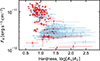 |
Fig. D.1. 0.2−2 keV observed flux, FX against an estimate of the spectral hardness (log[A1/A2]) during the early time NICER observations presented in Fig. 4. When FX is higher, the spectrum becomes harder. The red markers denote observations obtained when the source exhibited large amplitude modulations during W1. A smaller log[A1/A2] value denotes a harder X-ray spectrum. |
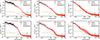 |
Fig. D.2. Power-law (tbabs*zpowerlaw, top row) and double blackbody (tbabs*(zbbody+zbbody), bottom row) model fits to the convolved eROSITA spectra (eRASS2, left column; eRASS3, middle; eRASS4, right), with J2344 being observed in eRASS2, eRASS3 and eRASS4 at 10, 192 and 378 days after optical peak. The black and grey markers represent source and scaled background spectra. The solid red line denotes the median model, whilst the shaded red band encloses 68% of the posterior, and the gold line denotes the median background model fit. Spectra are re-binned to minimum 10 counts per bin for plotting purpose only. The preferred model fit for the eRASS2 spectrum is the double blackbody model, whereas the power-law model is preferred for the eRASS3 and eRASS4 spectra. |
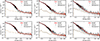 |
Fig. D.3. Absorbed power-law (tbabs*ztabs*zpowerlaw, top row) and double blackbody (tbabs*(zbbody+zbbody), bottom row) model fits to the convolved XMM spectra (XMM1, left column; XMM2, middle; XMM3, right). The preferred model fit for XMM1 and XMM3 is the dual black body model, whereas it is the absorbed power-law model for XMM2. XMM1, XMM2 and XMM3 were obtained at 36, 196, and 393 days after optical peak. |
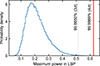 |
Fig. D.4. Distribution of maximum observed powers in the LSPs computed from each synthetic light curve. The solid red line marks the maximum power in the LSP computed from the observed 0.2−2 keV light curve (Fig. 7), whilst the dashed grey lines are as defined in Fig. 7. |
Spectral models for the eROSITA and XMM spectra.
D.2. Significance of the NICER periodicity
The LSP (Lomb 1976; Scargle 1982) computed using a least-squares normalisation (VanderPlas 2018) and from the high cadence X-ray observations obtained between MJD 59215 and 59240 (Fig. 7) shows a clear peak at  days, with the uncertainty computed based on the FWHM of this peak. To further assess the statistical significance of this peak, we used the following framework:
-
The 0.2−2 keV X-ray light curve was first fitted with a Gaussian process using the celerite package (Foreman-Mackey et al. 2017), and as in Burke et al. (2021), with a damped random walk (DRW) kernel of the form k(tnm) = 2σ2exp( − tnm/τDRW), where tnm is the time separation between points n and m in the light curve, σ is an amplitude decay term, and τDRW the DRW timescale. From this Gaussian process regression, we infer
 and
and ![Mathematical equation: $ \log[\tau_{\mathrm{DRW}}/\mathrm{days}] = -0.24^{+0.16}_{-0.12} $](/articles/aa/full_html/2026/04/aa56400-25/aa56400-25-eq38.gif) .
. -
105 synthetic light curves were generated from the power spectral density of the fitted Gaussian process using the method in Timmer & Koenig (1995), before modifying their probability distribution function to match the observed light curves as in Emmanoulopoulos et al. (2013), using the lcsim package (Kiehlmann 2023). These synthetic light curves were then down-sampled to match the sampling pattern of the observed light curves.
-
For each synthetic light curve, we then computed its LSP using the same normalisation as above and measured its maximum power, Pmax. From the empirical distribution of Pmax (Fig. D.4), then we compute the false-alarm probability of measuring P ≥ Pmax, under the null hypothesis that there is no periodic component in the signal.
-
Only one of the synthetically generated light curves show a peak in their LSP as high as 0.62 (Fig. D.4), thus we consider the false-alarm probability to be 1 × 10⁻⁵ (roughly equivalent to a 4.2σ detection of periodicity).
However, we caveat this seemingly high significance detection with the issue that we have ultimately only observed a small number of putative cycles, due to the cutoff in NICER observations as the system entered sunblock. In addition, we caveat this with the fact that robust detections of quasi-periodicity in accreting SMBHs are notoriously challenging to obtain in cases where the light curves exhibit a low number of cycles. Lastly, our ability to model the continuum component of the power spectrum is severely hampered by the fact that the bulk of the light curve data available as input for celerite is dominated by the candidate quasi-periodic modulation signal. The DRW model parameters obtained here may be biased, as they describe a power spectrum containing only minimal red noise, and approaching white noise, over the bulk of the temporal frequencies probed. Consequently, these false-alarm probabilities are very likely biased downward.
Appendix E: Photometric evolution
The general rise and decay evolution of J2344 in the optical, is broadly consistent with the observed behaviour of other optically-bright TDEs, with a comparison to a recent sample of ZTF-selected TDEs (Hammerstein et al. 2023) presented in Fig. E.1. With a peak c-band absolute magnitude of ∼-21.9, J2344 is one of the most luminous observed TDE candidates identified to date, although this is still three mags fainter than the extreme accretion event AT2021lwx (Wiseman et al. 2023). We note that there is a dearth of TDE candidates identified with peak absolute magnitudes approximately between -20 mag and -22 mag (Fig. E.1), and although such events are intrinsically rarer in the local universe (van Velzen 2018), the reasons for such extreme luminosities are currently unclear.
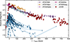 |
Fig. E.1. Comparison of the ATLAS o-band light curve of J2344 with the ZTF g-band light curves of the sample of optically-selected TDEs (blue markers) in Hammerstein et al. (2023). |
X-ray spectral fit results for the best-fitting models shown in Figs. D.2 and D.3.
All Tables
X-ray spectral fit results for the best-fitting models shown in Figs. D.2 and D.3.
All Figures
|
Fig. 1. Multi-wavelength light curve evolution of J2344, with the unabsorbed 0.2−2 keV fluxes (top panel) and the optical and UV fluxes (middle). Triangular data points denote 3σ upper limits on the flux. The horizontal dashed red line in the X-ray light curve panel denotes the 3σ upper limit on the 0.2−2 keV flux inferred from the non-detection of J2344 in eRASS1 (Homan et al. 2023), approximately 200 days before optical peak. The radio evolution (bottom panel) is well described by an expanding synchrotron-emitting region from a single ejection of material, consistent with an outflow launched by a non-relativistic TDE (Goodwin et al. 2024). |
| In the text | |
|
Fig. 2. Zoomed-in view of the X-ray evolution during the high-cadence NICER observations. The two panels have the same y-axis and cover the same amount of time on the x-axis. The different shaded backgrounds denote windows W1, W2, and W3 for the NICER observations (Sect. 3.1.3), taken 50−60 days, 60−70 days, and 165−210 days after optical peak. |
| In the text | |
|
Fig. 3. Joint evolution of the observed 0.2−2 keV flux (top panel) and the photon index (bottom panel) over time. The dashed red line marks the 3σ flux upper limit inferred from the non-detection in eRASS1. The X-ray spectrum remains ultra-soft (Γ ≳ 4) over the ∼760 days of X-ray monitoring (∼800 days after optical peak; Homan et al. 2023). |
| In the text | |
|
Fig. 4. Top panel: Evolution of the 0.2−2 keV flux, FX, over time during the high-cadence NICER observations at early times (∼50 days after optical peak). Second panel: spectral hardness estimated as log[A1/A2], with A1 and A2 the normalisation of the softer and harder blackbody components, respectively. Since smaller log[A1/A2] values correspond to harder spectra, J2344 exhibits a harder-when-brighter behaviour. Third and fourth panels: log A1 and log A2 in units of L39/[D10(1 + z)]2, with L39 the luminosity in 1039 erg s−1 and D10 the distance to the source in units of 10 kpc. Bottom panel: Evolution of the blackbody temperatures for each model component. The kT1 (orange) and kT2 (blue) were constrained to the 35−55 eV and 100−140 eV ranges during fitting. |
| In the text | |
|
Fig. 5. Power-law decay (red) and exponential decay (blue) models fitted to the 0.2−2 keV X-ray light curve of J2344 (excluding the early-time NICER data that exhibit modulations). The late-time flattening in the X-ray fluxes is better fitted by the power-law model here. |
| In the text | |
|
Fig. 6. Zoom in on the hours-timescale stochastic X-ray variability during W2, after the shut-off of the large amplitude modulations. The two dashed red lines are separated by ∼3 hours, and the X-ray flux varies by a factor of 2 between these observations. |
| In the text | |
|
Fig. 7. LSP computed from the 0.2−2 keV light curve between MJD 59215 and 59240. The dashed red line marks the period |
| In the text | |
|
Fig. 8. Folded 0.2−2 keV flux light curve (top panel) and hardness (bottom panel) of the NICER data from W1. In each modulation, the X-ray spectrum softens (higher log[A1/A2]) when the flux drops. The data points are coloured based upon which modulation they are associated with – M1, M2, or M3 – with M1 starting at MJD = 59220.3, and the light curves are folded with a periodicity of 3.05 days (this is consistent with the periodicity estimate of |
| In the text | |
|
Fig. 9. Precession (top panel) and alignment (bottom panel) timescales for a global precessing disc, plotted against black hole spin (a) for three stars of different masses being disrupted, assuming log[MBH/M⊙] = 7.2 (Appendix A). The shaded regions enclose the uncertainty on each timescale due to the 1σ uncertainty on log[MBH/M⊙]. These timescales were computed with H/R = 0.1 and α = 0.1, following Franchini et al. (2016). The dashed red line in the top panel denotes the observed 3-day modulation timescale observed in J2344, and the vertical grey lines denote the spin values that make Tprec consistent with 3 days (e.g. a ∼ 0.6 for a Sun-like star), highlighting that spin constraints derived from this approach are sensitive to the assumed mass of the disrupted star. |
| In the text | |
|
Fig. D.1. 0.2−2 keV observed flux, FX against an estimate of the spectral hardness (log[A1/A2]) during the early time NICER observations presented in Fig. 4. When FX is higher, the spectrum becomes harder. The red markers denote observations obtained when the source exhibited large amplitude modulations during W1. A smaller log[A1/A2] value denotes a harder X-ray spectrum. |
| In the text | |
|
Fig. D.2. Power-law (tbabs*zpowerlaw, top row) and double blackbody (tbabs*(zbbody+zbbody), bottom row) model fits to the convolved eROSITA spectra (eRASS2, left column; eRASS3, middle; eRASS4, right), with J2344 being observed in eRASS2, eRASS3 and eRASS4 at 10, 192 and 378 days after optical peak. The black and grey markers represent source and scaled background spectra. The solid red line denotes the median model, whilst the shaded red band encloses 68% of the posterior, and the gold line denotes the median background model fit. Spectra are re-binned to minimum 10 counts per bin for plotting purpose only. The preferred model fit for the eRASS2 spectrum is the double blackbody model, whereas the power-law model is preferred for the eRASS3 and eRASS4 spectra. |
| In the text | |
|
Fig. D.3. Absorbed power-law (tbabs*ztabs*zpowerlaw, top row) and double blackbody (tbabs*(zbbody+zbbody), bottom row) model fits to the convolved XMM spectra (XMM1, left column; XMM2, middle; XMM3, right). The preferred model fit for XMM1 and XMM3 is the dual black body model, whereas it is the absorbed power-law model for XMM2. XMM1, XMM2 and XMM3 were obtained at 36, 196, and 393 days after optical peak. |
| In the text | |
|
Fig. D.4. Distribution of maximum observed powers in the LSPs computed from each synthetic light curve. The solid red line marks the maximum power in the LSP computed from the observed 0.2−2 keV light curve (Fig. 7), whilst the dashed grey lines are as defined in Fig. 7. |
| In the text | |
|
Fig. E.1. Comparison of the ATLAS o-band light curve of J2344 with the ZTF g-band light curves of the sample of optically-selected TDEs (blue markers) in Hammerstein et al. (2023). |
| In the text | |
Current usage metrics show cumulative count of Article Views (full-text article views including HTML views, PDF and ePub downloads, according to the available data) and Abstracts Views on Vision4Press platform.
Data correspond to usage on the plateform after 2015. The current usage metrics is available 48-96 hours after online publication and is updated daily on week days.
Initial download of the metrics may take a while.