| Issue |
A&A
Volume 708, April 2026
|
|
|---|---|---|
| Article Number | A180 | |
| Number of page(s) | 16 | |
| Section | The Sun and the Heliosphere | |
| DOI | https://doi.org/10.1051/0004-6361/202557126 | |
| Published online | 08 April 2026 | |
High-resolution observations of small-scale activity in coronal hole plumes
1
Max Planck Institute for Solar System Research, Justus-von-Liebig-Weg 3, 37077 Göttingen, Germany
2
Institut für Sonnenphysik (KIS), Georges-Köhler-Allee 401A, 79110 Freiburg, Germany
3
Institut für Geophysik und extraterrestrische Physik, Technische Universität Braunschweig, Mendelssohnstrasse 3, 38106 Braunschweig, Germany
★ Corresponding author: This email address is being protected from spambots. You need JavaScript enabled to view it.
Received:
5
September
2025
Accepted:
1
February
2026
Abstract
Context. Largely radial ray-like structures, termed plumes, are often observed in coronal holes. Plumes have been proposed to channel magnetohydrodynamic (MHD) waves and the solar wind into the heliosphere. High-speed propagating disturbances (PDs), though well detected in plumes, cannot yet be clearly assigned to MHD waves or to mass flows. Additionally, plume bases as observed in the extreme ultraviolet are riddled with small-scale transients, which could be related to PDs.
Aims. We studied three plumes within an equatorial coronal hole observed by the EUV High Resolution Imager (HRIEUV) of the Extreme Ultraviolet Imager (EUI) on board Solar Orbiter. The properties of small-scale brightenings at the plume bases were investigated to interpret their nature and the possible relation with PDs in plumes.
Methods. A 30 Mm × 30 Mm sub-region is selected for each plume base. We processed the images with the difference of Gaussians (DoG) method to highlight the target brightenings, which were further identified with two different approaches. In the 30 minute observation, 50 brightenings were visually selected, which also helps to set thresholds for automatic detection, where we found 451 brightenings. Their properties, including apparent velocities on the plane of sky (PoS), were analyzed statistically. Potential field extrapolation based on the magnetic field data from the Polarimetric and Helioseismic Imager on board Solar Orbiter was used for correcting the PoS velocity to the real velocity along the magnetic field.
Results. We observe that the majority of base brightenings are small scale (with an area of less than 1.3 Mm2), short lived (lasting less than five minutes), and slightly elongated at the plume bases. They display intricate movements, with most showing velocities less than 10 km s−1 on the PoS. The velocity distribution of the base brightenings selected via visual identification shows a peak at 6–7 km s−1, while that of the automatically detected base brightenings peaks at a lower velocity of less than 5 km s−1. Their 3D velocities are found to be substantially lower than (and difficult to reconcile with) the speeds detected at greater heights in the plumes.
Conclusions. A direct link between base brightenings and PDs remains inconclusive due to the huge difference between their velocities. We propose two possibilities for base brightenings: they may be related to wave-driven Type I spicules or originate from interchange reconnections. Further investigation is required to validate these hypotheses.
Key words: Sun: corona / solar wind / Sun: UV radiation
© The Authors 2026
 Open Access article, published by EDP Sciences, under the terms of the Creative Commons Attribution License (https://creativecommons.org/licenses/by/4.0), which permits unrestricted use, distribution, and reproduction in any medium, provided the original work is properly cited.
This article is published in open access under the Subscribe to Open model.
Open access funding provided by Max Planck Society.
1. Introduction
Coronal hole plumes (hereafter plumes) generally appear as extended ray-like structures within a coronal hole. Their observations can be traced back to the early 20th century, and a large number of studies have been conducted on plumes (see review by Poletto 2015). Plumes expand super-radially into the outer solar atmosphere to more than 30 R⊙ (Woo & Habbal 1997; DeForest et al. 2001). They are found to be cooler and denser compared to the ambient interplume regions (Ahmad & Withbroe 1977; Wilhelm et al. 1998; DeForest et al. 2001; Wilhelm 2006). Once a plume forms, it can last for tens of hours (Lamy et al. 1997) to days (Young et al. 1999) with successors appearing at the same positions in weeks (DeForest et al. 2001).
Plumes are observed in visible light (e.g., Saito 1956), in extreme ultraviolet (EUV) (e.g., Ahmad & Withbroe 1977; Walker et al. 1993), and in soft X-rays (e.g., Ahmad & Webb 1978). Due to the observing geometry (from or close to the ecliptic plane) and generally large sizes of polar coronal holes (low background), polar plumes are easier to observe projecting well beyond the limb of the Sun, indicating the inhomogeneity of the outer solar atmosphere and providing information on the general magnetic field of the Sun (Shimooda 1958). However, tracing plumes in low-latitude coronal holes to greater heights is more difficult because of the much higher background from the nearby quiet sun and, often, active region areas. Nevertheless, these plumes are best observed against the disk, in ultraviolet and EUV emissions (e.g., Wang & Sheeley 1995b; Wang & Muglach 2008).
Plumes are found to be closely related to the chromospheric network, which is the pattern that outlines the convective supergranular cells. Newkirk & Harvey (1968) proposed that the rosette structures at the intersection of the networks lies at the root of plumes. Data from the Solar and Heliospheric Observatory (SOHO; Domingo et al. 1995) have revealed strong evidence of the spatial coherence of polar plumes and the network (DeForest et al. 1997). Gabriel et al. (2009) proposed that observations of “curtain plumes” can be modeled by microplumes that appear in the 5 Mm width boundaries of supergranular cells. It has been suggested by Wang & Sheeley (1995a) that the magnetic flux concentrated at the edges of network cells reconnects with the small bipoles pushed there by horizontal supergranular convective flows to produce plumes (see also Wang 1998 for a schematic).
Fast solar wind, which is also believed to originate from coronal holes (Krieger et al. 1973; Zirker 1977; Gosling & Pizzo 1999; Hassler et al. 1999), is possibly sustained, at least in part, by coronal hole plumes. Indirect support for this scenario may come from the relation between coronal upflows and network junctions. In fact, Hassler et al. (1999) found a correlation between Doppler shifts in the Ne VIII 770 Å line and the chromospheric magnetic network identified in the Si IIλ 1533 Å line. Their work indicated outflows with radial velocity on the order of 5–10 km s−1 in the network boundaries and of 10–20 km s−1 at the intersections of the boundaries. Tu et al. (2005) suggested that the Doppler velocity patches are related to magnetic funnels, which, at least in some cases, could be related to plumes. Despite the above evidence, it remains uncertain whether plumes are a source region for fast solar wind considering the estimation that plumes occupy 10% of the volume of polar coronal holes, providing only 15% of the mass (Ahmad & Withbroe 1977).
To help establish the possible contribution of plumes to the solar wind, it is essential to measure the speed of plume outflows at different heights. Numerous studies have been conducted over the years (e.g., Habbal et al. 1995; Corti et al. 1997; Wilhelm & Bodmer 1998), with different measurement methods and have yielded widespread conclusions. Off-limb plumes, for example, were investigated with the Doppler dimming method (Noci et al. 1987). Gabriel et al. (2003, 2005) proposed a velocity greater than 60 km s−1 in plumes from 1.05 to 1.4 R⊙, exceeding that in the interplume regions. However, Teriaca et al. (2003) found that static plumes in the outflowing interplume nicely reproduce the observational lines. In the low corona, some studies measuring the Doppler shift of lines in SUMER data failed to retrieve any obvious signature of outflows in plumes (Hassler et al. 1999; Hassler 2000; Wilhelm et al. 2000). In Feng et al. (2009), the stereoscopic reconstructions of the polar plumes corrected the line of sight (LoS) velocity measured spectroscopically in the O VI 1032 Å and 1038 Å lines to values along the plume directions that are still below 10 km s−1. On the other hand, analyzing observations of plumes in multiple spectral lines by the EUV Imaging Spectrometer (EIS; Culhane et al. 2007) on board the Hinode satellite (Kosugi et al. 2007), Fu et al. (2014) concluded that plume outflows are quasi-steady with a velocity increasing with height and can be an important source of solar wind. A summary of both the outflow speeds obtained there and from the previous literature can also be found in this paper.
Polar jets, observed at both X-ray (Shibata et al. 1992) and EUV (Alexander & Fletcher 1999) wavelengths, have been found to be precursors of plumes (Raouafi et al. 2008). The Atmospheric Imaging Assembly (AIA; Lemen et al. 2012) on board the Solar Dynamics Observatory (SDO; Pesnell et al. 2012) opened a new era in the study of plumes. Instead of being a spatially coherent “haze”, plumes were seen to be formed of filamentary fine structures, the so-called “plumelets” (Uritsky et al. 2021). In addition, numerous small jets (the so-called jetlets) and plume transient bright points (PTBPs) have been reported to occur in plumes (Raouafi & Stenborg 2014; Pant et al. 2015; Panesar et al. 2018; Kumar et al. 2022; Chitta et al. 2023b). Raouafi & Stenborg (2014) also proposed that these small-scale energy releases may sustain the evolution of plumes in the long term.
Propagating disturbances (PDs) are observed in plumes as quasi-periodic temporal fluctuations of brightness. They are found to move outward along the plume filamentary structures with speeds varying from a few 10 km s−1 to over 200 km s−1. However, their physical nature is not yet fully understood. On the one hand, PDs are thought to be caused by mass flows (McIntosh et al. 2010; Tian et al. 2011). On the other hand, in many studies, they are interpreted as signatures of magnetosonic waves (DeForest & Gurman 1998; Ofman et al. 1999; Banerjee & Krishna Prasad 2016; Banerjee et al. 2021). However, using multi-channel observations, Pucci et al. (2014) found that the PDs have higher speeds at lower temperatures, which is inconsistent with the wave scenario. More recently, Kumar et al. (2022) suggest the coexistence of strong flows and waves in plumes.
Several recent studies have focused on the dynamic processes at the bases of plumes and their connection to jetlets and PDs along plumelets. In particular, SDO/AIA and IRIS observations have revealed quasiperiodic energy releases with characteristic periods of 3–5 minutes in coronal-hole plumes (Kumar et al. 2022). They identified recurrent brightenings at plume bases and associated jetlets moving along plumelets. They also examined the magnetic topology and proposed a mechanism describing how quasiperiodic reconnection drives jetlet formation. In addition, the periodicities of these base reconnection events match those of microstreams and switchbacks observed by Parker Solar Probe, suggesting a potentially common origin for both phenomena (Kumar et al. 2023). Both works also show the chromospheric or transition region counterparts of these jetlets in AIA 304 Å, which appear to be less elongated than their hotter components. These findings are consistent with Uritsky et al. (2023), who suggest that these outflows are generated by impulsive interchange reconnection and likely constitute the primary source of mass and energy for the fast solar wind. However, recent magnetohydrodynamic (MHD) simulations have revealed that interchange reconnection is not a requirement for plume-related jetlets. In particular, energy conversion at the chromospheric and coronal interfaces of unipolar magnetic field threading plumes could play an important role in driving upflows (Bora et al. 2025).
Nevertheless, various studies have shown that the fine internal structures in plumes, such as brightenings, jetlets, and plumelets, might be intrinsically linked and drive the formation and evolution of the entire plume, and thus possibly contribute to the solar wind. However, due to resolution limitations, previous investigations on brightenings at plume bases have focused primarily on their temporal intensity variations. Unraveling the detailed morphological evolution of base brightenings and their direct link to plume outflows requires observations with high spatial and temporal resolution. Observations by the ESA and NASA Solar orbiter mission (Müller et al. 2020), acquired near one of the closest perihelia at about 0.3 au, provide unprecedented information on fine-scale structuring and small-scale dynamics in plumes. Given that the nature of small-scale activities at plume bases is not yet conclusively known, we refer to them as “base brightenings”, based on our observations.
In this work, we focus on analyzing the characteristics and movements of these dynamic base brightenings using high-resolution data from the High Resolution Extreme Ultraviolet telescope (HRIEUV), which is part of the Extreme Ultraviolet Imager (EUI; Rochus et al. 2020) on board Solar Orbiter. More details about the observations can be found in Section 2. In Section 3 we explain two different methods of capturing base brightenings and describe all the properties analyzed. This is followed by Section 4, where we show the statistical results and compare velocities of both base brightenings and PDs. The correction of plane of sky (PoS) velocities into the effective velocity along field lines is presented in Section 5. Discussion about the nature of both base brightenings and PDs can be found in Section 6. Finally, we summarize our findings in Section 7.
2. Observation
To study the base regions of plumes, we selected an equatorial coronal hole captured by EUI on October 13, 2022, adjacent to active regions. Three plumes were embedded in the observed coronal hole section, south of NOAA 13105 and west of NOAA 13107. The observations were taken when Solar Orbiter was at a distance of 0.29 au from the Sun, and at an Earth Ecliptic longitude of about −107°. With its 17.4 nm filter, the HRIEUV instrument recorded a 30-minute imaging sequence from 17:00:00 UT to 17:30:00 UT, at a cadence of 5 s with an exposure time of 2.8 s. The high temporal resolution is reduced to 20 s after binning four images together to reduce the noise level during data preparation. The HRIEUV images have an angular image scale of 0.492″ pixel−1, corresponding to about 100 km pixel−1 (a spatial resolution of about 200 km) at 0.29 au. The same dataset was used by Chitta et al. (2025) to investigate small jets in interplume regions.
In Figure 1a, we show an image of the Sun provided by the FSI of EUI on Solar Orbiter at 17:10:50 UT. The FSI observed the full disk of the Sun at a spatial resolution of about 1800 km and a cadence of 10 minutes. Available observations cover the whole lifetime of these plumes. Since here we focus on the small dynamic activity in solar plumes, we mainly use high resolution images from HRIEUV. The box in panel (a) indicates the region covered by HRIEUV, shown in panel (b). To enhance the plumes, which, even though brighter than their coronal hole background, are still much fainter than the surrounding active regions and quiet sun areas, we plot the images in panels (a) and (b) on a logarithmic scale. Zoom-in images of the base regions of the three plumes are shown in panels (c)-(e).
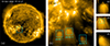 |
Fig. 1. Overview of coronal hole observations. (a) Full-disk image of the Sun provided by Full Sun Imager (FSI) of EUI. The box indicates the region covered by HRIEUV. (b) Image taken by HRIEUV with three boxes showing the base regions of the three plumes shown in panels (c)-(e). Both (a) and (b) are plotted in logarithmic scale in brightness. (c)-(e) Zoom-in normalized images of the base regions of the three plumes. (The associated movie is available online.) |
As shown in Figure 1(a), these three plumes are rooted in an equatorial coronal hole in the southern hemisphere. The positions of these plumes are close to the disk center with a heliocentric separation angle of about 25°, which allows observations of the base region with relatively low distortion. Meanwhile, at greater heights, the strong magnetic fields of the active region to the north could push the plume magnetic field southward. Thus, the resulting EUV emission from the plume appears to be more parallel to the PoS, which is better suited to study the movements of the fine structures in the plumes. The FSI sequences show that all the plumes have been in existence for more than one day and will disappear in about 20 hours after this HRIEUV observation period, while plume 3 appears to be already in its decay phase.
Comparing the three plumes, we find that features labeled 1 and 2 share similar characteristics in that both are located near the boundary of the active region with a north to south orientation. Plume 3 is rooted in the interior section of the coronal hole and is oriented in a north-east to south-west direction. Plume 1 and 2 are also brighter than plume 3. Considering that plume 3 is already decaying, this agrees with the suggestion in Pucci et al. (2014) that plumes die as their gas density is reduced. Despite these differences, all plumes have highly dynamic base regions with brightenings appearing near their footpoints and moving outwards.
3. Data analysis
3.1. Visual identification method
To better capture the moving bright features in the base regions of the plumes, we first applied a visualization-based method. Before detailed analysis, we prepared the data by averaging four consecutive images and then applying a running average over 3 × 3 pixels to each resulting image to reduce noise. We normalized each base region (see Figure 1c-e) to the maximum and minimum intensities of the whole sequence in each sub-region to make the data from the three plumes directly comparable. Here, we applied the difference of Gaussians (DoG) method, which is an image processing technique used to enhance edges or features in an image by highlighting areas of rapid intensity change (Lindeberg 1994; Lowe 2004). It involves subtracting two Gaussian-blurred versions of the same image. In our study, we used two Gaussian kernels with σ = 3 pixel and σ = 5 pixel, respectively. Different thresholds on DoG maps have been tested and we used 0.01 (see Appendix A) as a reasonable number to cover brightenings as much as possible while avoiding connections of brightenings close to each other.
Contours representing the target base brightenings at different times are overplotted on the same images to show the trajectory of them. Figure 2 shows plume 2 as an example. To reduce overlap, the entire observational sequence (30 min) is divided into four distinct time intervals, each covering specific enhancements in the light curve of the base region (see Figure 2a). Panels (b)-(e) show the brightening contours obtained with the thresholds of 0.01 on DoG maps in four different time periods. Brightenings appearing at different times are marked with different colors (see the color bars in Figure 2). In these images, the “gradient patterns” (the overlapping contours with changing colors; see examples in red boxes in Figure 2) indicate the moving structures. Using these “gradient patterns” as a guide for the eye, we checked the images for moving brightenings. Some brightenings existing in two time spans were checked throughout their whole lifetimes and still counted as the same ones. With this method a total of 50 base brightenings was selected in the three plumes.
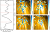 |
Fig. 2. Dynamics at the base of plumes. (a) A sample light curve obtained from the base region of plume 2 (see Figure 1(d)). The whole time period (30 min) is divided into four sections (partitioned at orange dashed lines). (b) – (e) Images of the base region of plume 2 acquired at the middle instance from each temporal section in (a). Brightenings identified using chosen thresholds are marked by the contours (colors indicate time progression; as defined by the color bars). The red boxes highlight several examples of the “gradient patterns”, which are formed by contours from successive frames being adjacent to or overlapping one another, thereby illustrating the movement of the brightenings. Note that, even though we have divided the entire observation into four sub-periods, the contour of the brightenings that appears later will inevitably overlap the ones that appear earlier. For example, a discrete contour could be either a brightening that only appears in one frame, or a brightening that does not show a significant movement. |
For each base brightening, a local background was subtracted, calculated around its position as the minimum value at each pixel along its lifetime. After removing the background, the base brightenings show up better and their boundaries are then redefined by using a new threshold of 0.75 of their maximum value, after several thresholds being tested (see Appendix A).
3.2. Automatic method
The visual identification method allows us to select only those base brightenings which are relatively large and bright and experience noticeable shifts in positions. This likely introduces a selection bias. To mitigate this, we also implemented an automated selection method to detect brightenings in the three plume bases. The same as for the visual identification method, we applied the DoG method to each averaged image and started with a threshold of 0.01 in the enhanced images. All pixels with a value higher than this threshold are labeled as “bright pixels”. In each frame, connected bright pixels are considered as a single brightening by performing a four-neighbor search. Small fragments of less than 2 × 2 pixels are ignored.
For each detected brightening, we examined the subsequent image frame to track its temporal evolution. If a new brightening larger than 2 × 2 pixels appears within a defined neighborhood of the previous brightening, we interpret both as part of the same evolving structure observed at different times. This neighborhood is defined as a region centered on the brightening peak in the previous frame with a radius of 6 pixels. The process was repeated in subsequent frames based on the newly-evolved brightening until the brightening becomes unrecognizable. Considering the pixel size of 100 km and the time cadence of 20 s, the threshold of 6 pixels corresponds to a velocity of 30 km s−1. More details on threshold selection can be found in Appendix A. We ignored the brightenings that appear in only one frame.
A total of 451 base brightenings are detected with this method. Their boundaries are also redefined as 0.75 of the maximum value of the base brightenings after the local background being removed. The positions of all base brightenings are shown in Figure 3 where diamonds indicate the positions of the intensity-weighted centers of each base brightening during its temporal evolution, the color representing its start time. The detected base brightenings are also compared with those we detected by visual identification, and 48 out of 50 of those selected manually are also captured using the automatic method. However, fluctuations in brightness over time and the spatial proximity of different base brightenings can result in discrepancies in some events.
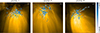 |
Fig. 3. Zoom into the plume bases observed on October 13, 2022 17:10 UT. The intensity-weighted center of each base brightening along the evolution is overplotted on the images. The color represents the time of the first appearance of each base brightening (see the color bar). |
3.3. Properties
For all base brightenings selected with both methods, we investigated their properties (area, lifetime, intensity, length-to-width ratio, and velocity) statistically. Based on their boundaries, defined on images with background subtracted as described above, we can easily get the area and average intensities, which are defined at the maximum along the evolution of each base brightening. Here we calculated the mean intensity with and without removing the local background. Lifetime is the time difference between the first and last appearance of a base brightening with an accuracy of 20 s. This lifetime can be considered as an upper limit because it assumes that the base brightening appears at the beginning of the first exposure and disappears at the end of the last one. However, the lifetime of the base brightenings that already exist at the start or remain at the end of the timeseries is underestimated. Considering that only 5% of events are influenced and the longest-lived ones have a lifetime shorter than 5 min, this effect can hardly have a significant impact on statistical results.
We also studied the shape of the base brightenings, which is quantified as the length-to-width ratio when the area reaches its maximum along the evolution. This is calculated by fitting the outline of a base brightening with a 2D Gaussian function, and getting the ratio of full width at half maximum (FWHM) at both directions, namely, the major and minor axes, as a proxy.
The velocity, representing an apparent PoS motion of the base brightening, is calculated using its initial and final spatial locations. Considering that size, shape, and brightness change during its evolution, it is complex to find one representative point for a base brightening. We compared the positions of peak points, the centroid, and intensity-weighted centroid and find that statistically they are close enough to have negligible impact. We used the intensity-weighted centroid as the location of the base brightening to estimate the velocity, because it factors in both the extent and intensity.
4. Results
4.1. Visual detection results
We investigated several properties of the 50 base brightenings selected with the visual identification method described above, including intensity, lifetime, area, shape, and velocity. The distributions are shown in Figure 4. Panel (a) indicates that the mean intensities of the base brightenings show different peaks in different plumes. However, as seen in panel (b), they merge closer when the local background is removed. This tells us that although the base brightenings in bright plumes have higher intensities than those in faint plumes, the difference is mainly caused by the overall brightnesses of the plumes.
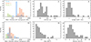 |
Fig. 4. Distributions of the properties of the base brightenings selected with the visual identification method (50 base brightenings). (a) shows the mean intensity of the base brightenings without subtracting the local background while (b) shows the mean intensity with the local background removed. (c) – (f) show the lifetime, area, length-to-width ratio, and velocity. The velocity here is a projection on the PoS and is calculated using the first and last positions of the intensity-weighted center of the base brightening. |
Most of these base brightenings are transient and small scale, as shown in Figure 4c and d. They mostly have a lifetime of less than 5 minutes. The short-lived ones have a lifetime of 60 s. Note that the method we use only allows us to spot brightenings appearing in several images consecutively. The area of the studied base brightenings varies from 0.05 to 1.3 Mm2. These values are based on the threshold used to demarcate the brightenings’ boundaries. The distribution of the length-to-width ratio (Figure 4e) shows a clear peak at around 2 and can reach 8. This means most base brightenings exhibit a slightly elongated elliptical morphology while a minority exhibit significant elongation, forming a plumelet-like structure at low altitudes.
Figure 4f shows the velocity distribution. About 70% of the base brightenings have a velocity component in the PoS of less than 10 km s−1. The velocity histogram peaks around 6 km s−1. By closely examining the trajectories of these structures, we find that their movements are more complex than unidirectional following the plume threads. Typically, the base brightenings appear closer to the footpoint and move outward, away from the base region. Although some of the structures move in alignment with the plume (i.e., from north to south in plumes 1 and 2), some deviate from this direction. Considering an open magnetic flux tube with a funnel-shaped structure, in which the magnetic field lines that start from a concentrated region in the photosphere expand nearly horizontally in the chromosphere and transition region, forming a canopy, before becoming more vertical again on the way to the corona (Solanki & Steiner 1990; Schrijver & Title 2003). There could also be small-scale loops in the neighborhood in addition to these open field lines. In such a geometry, depending on which field line the base brightening is moving along and at which height, it can show different apparent movements in PoS. Furthermore, both the intensity of the base brightenings and the directions of their motion can change throughout their evolution owing to variations in photospheric magnetic field on short timescales of less than 5 minutes (e.g., Anusha et al. 2017; Chitta et al. 2023a).
4.2. Automatic detection results
The same properties are also studied for the base brightenings captured by the automatic method. In Figure 5 we show a comparison of the distributions of the properties of the base brightenings obtained by visual identification and the automatic method. Both methods produce similar results, that is, most of the studied base brightenings are small scale, transient, and exhibit slightly elongated morphologies.
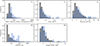 |
Fig. 5. Normalized distributions of the properties (mean intensity, lifetime, area, length-to-width ratio, and velocity) of the base brightenings detected with both visual identification method (50 base brightenings) and automatic method (451 base brightenings). The gray bars show the results from the automatic method and the blue line-filled bars show the results from the visual identification method. |
Apart from the similarities, the automatically-detected base brightenings show peaks at smaller intensity, area, lifetime, and velocity. This means that the automatic method is capable of picking up fainter, smaller, and shorter-lived brightenings. These brightenings appear more often than the ones selected manually. Since we neglect the brightenings that only appear in one frame, the deduced lifetime cannot be shorter than 40 s. More than 40% of the automatically identified base brightenings possess this minimum lifetime. The distributions of length-to-width ratio show less difference as we did not have a preference in the shape of the base brightenings when we selectred them by eye, but automatically detected ones still show a slightly higher rate of circular morphology.
Most base brightenings move with a velocity of less than 10 km s−1, irrespective of the detection method. Compared with the visual identification method, the automatic method detects more base brightenings (50%) moving with even lower velocity, less than 5 km s−1. For these, the distribution peaks at 3–5 km s−1. Note that, as we only use the first and last positions of each base brightening to get an average velocity, the small velocities could be caused not only by the slow motion but also by base brightenings moving in variable directions. We categorized all 451 base brightenings according to their directions of motion. Excluding the 191 short-lived base brightenings that appear in only two frames, for which a variation in the direction of motion cannot be defined, only 38 of the remaining ones have a relatively fixed direction of motion, i.e., the difference of their directions in two successive time intervals is always not less than or equal to ±30°. These events also exhibit relatively higher speed (see Table 1). Two peaks are found in their velocity distribution at 7 km s−1 and 13 km s−1. Meanwhile, the remaining 222 base brightenings show a more random-like motion.
Automatically detected base brightenings categorized according to directions.
4.3. Base brightenings and PDs
The velocities of the base brightenings are very small compared with the velocities of PDs within plumes. Previous studies suggest that apparent outward speeds range from several tens to 300 km s−1. A similar velocity can be detected in our work as well. In Figure 6, we take a long slit starting from the base region and following one of the bright threads in the plume to make a time-slice plot (see Figure 6b). The position of this slit is shown in Figure 6a. In this time-slice plot, one can clearly see the recurring base brightenings at the footpoint and the PDs following. We mark some of them that are easy to distinguish from the background with the straight dashed lines.
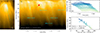 |
Fig. 6. (a) HRIEUV image of plume 2 showing the base region and plume streams. The overplotted box shows the position of the slice that is taken to form the time-slice plot shown in (b). (b) Time-slice plot. The PDs are marked with blue dashed lines. The average velocity is 112 km s−1. The red arrow points to one of the PDs, which is potentially transformed by a slow-moving base brightening. As an example, (c) shows the light curves at different distances (see different colors) of the first PD. The light curves are fitted with a Gaussian function. The central time (where the light curve peaks) derived from the fitting can be found in (d), together with the linear fitting of distances vs. central time. The error of intensity in (c) is calculated taking the readout noise and dark current into account. This error is propagated to get the error of central time in (d). (The associated movie is available online.) |
To calculate velocities, the light curves with an original time cadence of 5 s (and without spatial running average applied) of each PD at different distances along the slit are fitted by Gaussian functions. In Figure 6c, we show the light curves of the first PD, with different colors indicating different distances. The error bars come from the readout noise and dark current (see equation S1 in Chitta et al. 2023b). In this dataset, the exposure time is 2.8 s and the conversion factor of photons to DN is 7.29 DN photon−1. The temporal positions of the PD, where its light curve peaks derived from the fitting, are then linearly fitted to the distance (Figure 6d). The speeds are distributed over a wide range, from 80 to 160 km s−1. The slow ones have a similar velocity as reported in Gabriel et al. (2003, 2005), while none of the PDs in our dataset have a velocity as small as the 25 km s−1 reported by Fu et al. (2014). The LoS Doppler velocities at a height of about 20–40 Mm have been found to be 30–60 km s−1 (Hassler et al. 1997; Banerjee et al. 2000; Teriaca et al. 2003; Wilhelm 2006; Banerjee et al. 2009). For comparison, outflow velocity of PDs and small jets as measured in Pucci et al. (2014), Kumar et al. (2022), Chitta et al. (2023b) is in the range of a few 10 km s−1 to a few 100 km s−1.
In one case, we observed a brightening at the plume base propagating at a speed of about 10 km s−1, potentially transitioning to a PD moving at a higher speed of about 80 km s−1 (see the arrow in Figure 6b). This could be possible evidence that the base brightenings and PDs at greater heights are intrinsically related, but one such overlap may also occur purely by chance. In addition, their velocities are very different. However, as the velocities we measure here are components on the PoS, the comparison of the real velocities of the moving base brightenings and PDs should take projection effects into consideration.
5. Velocity correction
Based on our analysis of velocities, to assess the connection between base brightenings and PDs at higher altitudes, it is important to understand the apparent acceleration from a velocity of less than 10 km s−1 of most base brightenings to around 100 km s−1 of PDs. Since the coronal hole is adjacent to active regions, we expect that the strong magnetic field from the active regions will expand and influence the open fields, especially at a relatively high altitude. This could imply that, while the open magnetic field remains nearly radial (vertical) at the lower altitudes corresponding to the height of the base brightenings, it is more horizontal at the higher altitudes guiding the PDs. The bending of magnetic field lines can cause the illusion of acceleration because only the velocity component in the PoS can be captured in images. As we mentioned earlier, not all base brightenings move in a fixed direction. Since the ones with random-walk-like motions are possibly related to field lines that are closed or nearly horizontal before turning outward, we here focus on the base brightenings that appear to move following the same plume threads as PDs. The aim is to de-project the observed speeds of these base brightenings to determine their true velocities and assess whether these velocities align more closely with the speeds of PDs.
An extrapolation of magnetic field can help us to understand the 3D morphology of the magnetic field and to de-project the velocity component to the real velocity, assuming that the base brightenings move along the magnetic field lines. Here we used the vector magnetic data in the solar photosphere provided by the High Resolution Telescope (HRT), part of the Polarimetric and Helioseismic Imager on Solar Orbiter (SO/PHI; Solanki et al. 2020). The data were taken at 16:30 UT, 30 mins before the EUI observation with a high spatial resolution of about 200 km. In this dataset, HRT has a smaller field of view (FoV) than HRIEUV and is offset to the southeast.
After aligning the HRIEUV and HRT data, the region covered in both is shown in Figure 7a. The background image comes from HRIEUV at 17:00 UT and the contours of the LoS magnetic field with the level of 50 gauss are overplotted. It is clear that the roots of all plumes are closely related to magnetic concentrations spanning about 30 Mm. The ambiguity in the transverse field’s component of the SO/PHI-HRT vector magnetogram was removed using an adapted version of the Helioseismic and Magnetic Imager (HMI; Schou et al. 2012) (on board SDO) disambiguation pipeline (Hoeksema et al. 2014; Metcalf et al. 2006) that implements the minimal-energy disambiguation method ME0 (Metcalf 1994).
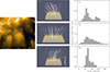 |
Fig. 7. Magnetic field imprints of the plumes. (a) Field of view covered by both HRIEUV and HRT data. The background image comes from the HRIEUV at 17:00 UT. The red (blue) contours of LoS magnetic field with the level of positive (negative) 50 gauss are overplotted. (b), (d) and (f) show the extrapolated magnetic field lines at the location of the three plumes, the sub-regions marked with boxes in (a), (c), (e), and (g) are histograms of frequency of the separation angle between the local magnetic field vector and LoS of three plumes. This separation angle is obtained as an average over all pixels at heights between 2000 and 4000 km along each field line; see the yellow boxes in (b), (d), and (f). |
We calculated the radial magnetic field based on the disambiguated vector magnetic data using the transformation in Gary & Hagyard (1990). With the radial magnetic field as the bottom boundary, we made a potential extrapolation to the height of 256 pixels (25 Mm). Figure 7b, d, and f separately show the field lines where the three plumes are located. The bottom slices are the magnetic field along the Z axis, which is the local vertical direction on the Sun. The extrapolation indicates that the open field lines related to the plume grow and expand to form a funnel structure, in agreement with both observations and previous simulations. The red lines in the boxes represent the direction towards Solar Orbiter.
Here, all field lines reaching the top boundary are regarded as open field lines. For each open field line, we calculated the angle between the magnetic field vector and LoS direction at different heights. In Figure 7c, e, and g, we show the distribution of the separation angle of each field line averaged over all positions between 2000 and 4000 km. It has been suggested by Berghmans et al. (2021) that the small-scale brightenings in the quiet sun observed by HRIEUV occur at heights around 2000–4000 km, although the brightenings at the plume base need not necessarily form at the same height as quiet sun brightenings. Depending on the morphology of each plume, the distributions peak at different angles, from 20° to 30°. This indicates that the velocity can be enlarged by at most a factor of 3 in the de-projection. This is not enough to explain the difference between the velocities of base brightenings and PDs. Although the fastest ones (with a velocity of 30 km s−1) could move at a speed almost reaching the high velocity of PDs, most base brightenings have a 3-dimensional velocity of less than 30 km s−1. In other words, instead of an illusion caused by perspectives, the difference between these velocities is real.
However, the same angle cannot be used for the correction of velocities detected at greater heights. Due to the limitation of HRT FoV, the adjacent active regions are not covered in this data. As mentioned before, the magnetic field from the active regions could push open field lines either toward them or away from them, depending on the magnetic polarity. This effect is missing in the potential extrapolation with HRT data. To demonstrate this effect, we ran another extrapolation test with data from HMI. It proves that this influence exists (Appendix B), although it is hard to quantify it. In summary, we believe that the angle between the direction of the PDs and LoS is likely to be greater than that of the base brightenings, that is, part of the difference between the apparent speed of PDs and base brightenings could come from the projection effect.
6. Discussion
6.1. Link between base brightenings and PDs
6.1.1. Are PDs mass flows or waves?
We can begin the discussion by examining the physical nature of PDs, which are better understood than base brightenings. This allows us to further investigate the potential link between the two, thereby contributing to a deeper understanding of base brightenings. In both coronal loops and plumes, PDs are widely interpreted as mass flows or waves. Previous studies suggested the existence of slow-mode waves in plumes (e.g., DeForest & Gurman 1998; Krishna Prasad et al. 2012). Such slow-mode waves have been invoked as potential contributors to coronal heating (DeForest & Gurman 1998; De Moortel et al. 2000; McEwan & de Moortel 2006). We first verify the wave interpretation using temporal variations of the intensity along the plumes in our observations. To this end, we select one of the distinct PDs (see Figure 8a) and select equally spaced points along this PD at different distances from the base region (see diamonds in Figure 8a). Through each point, we cut a slit perpendicular to the PD and fit a Gaussian function to the intensities along the slit. In Figure 8b, we show the amplitudes of the fitted Gaussian functions as a function of distance. A similar variation in intensity, initially increasing with height and then decaying, can be observed in other PDs as well.
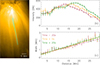 |
Fig. 8. Propagating disturbances. (a) HRIEUV image of plume 2. Positions at different distances from the base region are marked with diamonds. The intensities along the slits perpendicular to the stream direction at these positions are fitted by a Gaussian function. (b) and (c) show the peak and FWHM of the fitted Gaussian functions, as a function of the distance along the PD, at three instances (each separated by 20 s; as identified with different colors). Same as Figure 6c and d, the error of intensity in (b) comes from the detector readout noise and dark current and the error of width is derived from the Gaussian fitting. |
This helps characterize the nature of the PD. If the plumes are in hydrostatic equilibrium, we expect their EUV emission to fall off exponentially with a certain scale-height set by the pressure at their base. In our example, we observe that the EUV emission first increases up to several megameters above the base and then decreases. Moreover, we find that the peak position of the intensity shifts outward with time (see the variations of intensity with distance at three instances separated by 20 s). Both of these factors are inconsistent with plumes being in a hydrostatic equilibrium. These factors can only be reconciled with additional heating along the plume away from the base region or excess plasma cooling from higher temperatures. However, because we observe PDs propagating outward rather than downflows as typically expected in the case of plasma cooling, we suggest that our observations are consistent with a scenario of injection of material at the base of plumes. This intensity variation could also be explained by a temperature gradient along the direction of the PDs. However, this cannot be confirmed in the present study and has not been reported in previous data (Wilhelm et al. 2011).
Additionally, our analysis reveals PDs that exhibit speeds varying from 80 to 160 km s−1. Only the highest speed among them can reach the local acoustic speed cs ≈ 150 km s−1 at coronal temperature T = 106 K. Note that because of the projection effects the apparent velocities are only a lower limit of the real velocities. In an optically-thin atmosphere, it is possible that multiple PDs, with similar velocities close to the local sound speed but different inclinations over the PoS, could overlap along the LoS, giving the impression that different PDs have different speeds. However, considering that the slowest PDs in our sample travel at 80 km s−1, that is, half the sound speed, a separation angle from PoS of about 60° would be needed to reach the typical velocity of a slow mode. Thus, the slow-mode waves could explain the propagation only when the angles between the propagating directions of different PDs are relatively large. In summary, our results are more in favor of PDs being high speed mass flows than waves (see also Chitta et al. 2023b).
6.1.2. Mass conservation: evolution of base brightenings into PDs
Assuming that the PDs are mass flows, here we investigate the possibility that even the base brightenings are mass flows in their initial stage and eventually evolve into PDs. From the trajectories and velocity distributions of the base brightenings, we know that some of them, although only a small fraction (less than 10%), have a relatively fixed moving direction with a detectable velocity, which conforms to the motion of the outflows. Their velocity distribution peaks at around 7 and 13 km s−1, corresponding to the outflow velocity in coronal holes based on the Doppler shifts of the transition region Ne VIII emission line (Hassler et al. 1999). In addition, upward-propagating brightenings have also been found in AIA 304 Å channel, which can correspond to the chromospheric or transition region signatures of jetlets (Kumar et al. 2022, 2023). The existence of elongated base brightenings also proves that some of them are jet-like structures. However, the apparent “outflows” near the plume base do not share the same order of magnitude of velocity of plume flows detected at higher altitude. Despite previous work stating that jetlets (mass flows at the plume base) could move outward to form plumelets, in this work we find it difficult to reconcile the possibility that base brightenings are the same evolving structures as plume outflows.
If the base brightenings evolve outward to become plume outflows, they should have a nearly constant outward mass flow rate given by ṁ = vmeneA, at different heights, where v is the outflow velocity, me and ne are the electron mass and number density, and A is the cross-sectional area of the outflow. In the following paragraph, we estimate the changes in velocity, cross-sectional area, and number density.
From this work, we know that we could conservatively consider an increase in velocity (from about 30 km s−1 to 100 km s−1) of a factor of 3. To estimate the expansion rate, we studied the width change of the same PD selected in Figure 8a. In Figure 8c, we show the FWHM of the fitted Gaussian functions against the distance. The expansion factor at a very low altitude is difficult to measure directly from the observation. For that, the base region is too bright and dynamic to resolve plume streams. In the higher corona, where filamentary PD substructures can be observed, we find that these streams widen linearly with distance and the stream width can increase by at least a factor of 3 at a distance of 20 Mm relative to the base region, which gives an expansion factor of 9. To compensate for an increase in the velocity and cross-sectional area, a decrease in the density of a factor of 27 seems to be necessary in the PD to satisfy a constant mass rate. This disagrees with our observations as EUV emission, which depends on ne2 under a constant temperature assumption, does not show such a huge difference in the base region and plumelets. It is important to mention that the expansion rate can only be regarded as a rough estimation. In reality, most streams have diffuse edges that can hardly be measured precisely. However, even with a negligible expansion base regions cannot be three times denser than plumes at 20–40 Mm, which is consistent with results on plume density in the literature, as discussed below.
Different methods have been applied over the years to measure plume density. A summary of the results of such investigations can be found in Table 3 and Figure 17 of Wilhelm et al. (2011). The results are variable with large error bars. For example, Fludra et al. (1999) study polar plumes and find that the density decreases with height from 2 × 108 cm −3 at the limb to 6 × 107 cm −3 at 1.1 R⊙. Young et al. (1999) derive densities of 2.5–5.6 × 109 cm −3 in the bright base region and of 3.8–9.5 × 108 cm −3 above the limb at coronal temperature. Taking into account the power law fits, in both plume and interplume regions, ne is found to be proportional to (R⊙/R)8 below R = 2 R⊙ (Wilhelm et al. 2011). This empirically provides that the density at the plume bases is approximately 1.3 times the density at a height of 20–40 Mm. Although different densities are found in different cases, they do not seem to meet the possibility of mass flux conservation.
6.2. Decoding base brightenings
6.2.1. Hypothesis I: Reconnection
One possible explanation for the base brightenings is related to magnetic reconnection. Kumar et al. (2022) selected one of the large base jets and applied a potential-field extrapolation from an HMI magnetogram to study the magnetic topology of this region. They revealed that a fan-spine structure is involved in producing the brightening and outflow. Cho et al. (2023) showed evidence of associated brightenings and blueshifted plasma (outflows) in the region with opposite magnetic polarities and found a high temperature structure at the base of the plume. Uritsky et al. (2023) identified the power-law statistical distribution of these outflows as a signature of impulsive interchange reconnection. These works support the picture of interchange reconnection between open field lines and closed loops, leading to localized rapid enhancement and ejection of materials.
However, the necessity of this mechanism remains debated. As pointed out in the Introduction, according to MHD simulations of plumes, such an interchange reconnection scenario is not a requirement for plume-related outflows (Bora et al. 2025). Furthermore, previous observational studies have not discussed in detail the movement of the base brightenings. Instead, reconnection-driven jetlets are typically observed to propagate at much higher speeds, comparable to those of the PDs analyzed in this work. It is possible that it is limited by the resolution of previous EUV imaging observations, so that the movement of these very small brightenings was not easily captured. One possibility that might explain the observed motions is that frequent, repetitive, and impulsive reconnections take place and result in discrete brightenings flashing successively over a short period of time in a small region, creating the appearance of movement. Alternatively, movement may arise from the actual evolution of brightenings. For example, the plasma flowing along the newly-formed closed loop hits the footpoints of the loop, causing the evaporation of the chromospheric material to fill in the whole loop. In this work, we cannot corroborate whether magnetic reconnection has occurred. More magnetic field data are required to study the evolution of the photospheric magnetic field below the plumes. This hypothesis about reconnection depends on how mixed the magnetic polarities are, and the determination of this mixing depends on the instrument’s sensitivity and resolution.
6.2.2. Hypothesis II: Wave-driven Type I spicules
Although different forms of reconnection, as stated above, could explain the energetic and statistical properties of the plume jetlets, the dynamic behavior of the base brightenings themselves may suggest a more complex interaction with the lower atmosphere. Specifically, the slow and more random motions of the base brightenings, distinct from the outflows, suggest a potential link with direct photospheric drivers, such as spicules.
Spicules are cool and dense structures that are usually observed to be thin and elongated in Hα and other chromospheric lines. de Pontieu et al. (2007b) categorizes them into two types, Type I and Type II spicules. Type I spicules typically have lifetimes between 3 and 7 min and show up and downward motions along the magnetic fields with velocities of 20–50 km s−1. They are reported to be manifestations of the same driving mechanism associated with chromospheric shocks and photospheric oscillation (Hansteen et al. 2006; de Pontieu et al. 2007a). Recently, EUV signatures of dynamic fibrils, the on-disk counterparts of Type I Spicules, have been studied using Solar Orbiter observations (Mandal et al. 2023). In contrast, Type II spicules move upward rapidly with apparent speeds of 80–300 km s−1, have shorter lifetimes of 1–3 min and do not display clear downflows (de Pontieu et al. 2007b; Pereira et al. 2012, 2016).
Some observational similarities can be found between base brightenings and Type I spicules. Both show complex motions and have comparable velocities. In addition, both appear to be periodic and related to chromospheric network concentrations (Kumar et al. 2022). This can help us to understand the formation of base brightenings. Type I spicules are believed to be potentially triggered by shock waves powered by p-modes (e.g., De Pontieu et al. 2004). This omnipresent p-mode oscillation, as also reported in Kumar et al. (2022), can be the cause of base brightenings as well. Meanwhile, the velocities of the PDs are closer to those of Type II spicules. Both are outwardly oriented and fade out after a certain distance. It is also reported by Cho et al. (2023) that they may have matching periodicities, suggesting a close link between them.
It is worth mentioning here that the base brightenings do not show the back-and-forth motions typical of Type I spicules and dynamic fibrils. Also, the base brightenings discussed here are less elongated and have shorter lifetimes than chromospheric Type I spicules. This may be a consequence of the coronal hole environment. In coronal holes, where the magnetic field is more vertical, the leakage of p-modes is more difficult due to a shorter acoustic cut-off period, forming less-elongated and shorter-lived structures, like the base brightenings observed in this study.
7. Conclusion
In this study, we investigate in detail the small-scale dynamic brightenings in the base regions of three coronal hole plumes with the observation from HRIEUV. Here we find that 1) The majority of the observed brightenings at the base of plumes can be characterized by their small-scale nature (covering an area of less than 1.3 Mm2), transient behavior (with a lifespan of less than 5 minutes), and display of slightly elongated morphologies. 2) The intensities of base brightenings from different plumes are identical once the plume background is subtracted. 3) Base brightenings show complex movements. Most of them appear to move with a velocity component in PoS of less than 10 km s−1. After de-projecting the PoS velocities to 3-dimensional velocity using an extrapolation with SO/PHI data, we find the velocities of the base brightenings are still much smaller than those of the PDs.
For the potential explanations of the base brightenings, we first investigated the link between base brightenings and PDs, based on the two possible physical natures of the PDs, slow waves, and mass flows. Assuming a constant temperature along the plume, our results are more in favor of PDs being mass flows than slow waves. In that case, our mass conservation estimate does not support the base brightenings as the initial outflows that can evolve into high-speed PDs. Given the assumptions as well as the estimation errors involved, we cannot, however, conclusively rule out the possibility that base brightenings and PDs are directly linked. However, in the absence of such a connection, determining the nature of base brightenings on the basis of an understanding of PDs remains challenging. Therefore, we propose two hypotheses on the nature of base brightenings: (i) they are associated with wave-driven Type I spicules, or (ii) they are produced by interchange reconnection. Our study can provide very limited constraints on both hypotheses, highlighting the need for further detailed investigation. Considering the small size and short duration of these structures, observations with high spatial and temporal resolution are necessary, and longer continuous observations could also be helpful in studying the slow-mode wave scenario in plumes. Also, the present results are derived from observations in a single bandpass, and thus with limited temperature coverage. Future studies could take advantage of simultaneous observations from multi-instruments, that is, photospheric magnetic field data and spectral data, which provide information in different layers in the solar atmosphere. In this work, we see that magnetic field data can assist in correcting the observed PoS velocities. In addition, Doppler velocities derived from spectral data can also provide the LoS velocity component. These are essential for understanding the mechanism of plumes and measuring the proportion of released energy that is carried by outflows to reach the upper atmosphere and eventually contribute to the solar wind.
Data availability
Movies associated with Figs. 1 & 6 available at https://www.aanda.org
Acknowledgments
The authors thank the referee for helpful comments that have improved this paper. Solar Orbiter is a space mission of international collaboration between ESA and NASA, operated by ESA. The EUI instrument was built by CSL, IAS, MPS, MSSL/UCL, PMOD/WRC, ROB, LCF/IO with funding from the Belgian Federal Science Policy Office (BELSPO/PRODEX PEA C4000134088); the Centre National d’Etudes Spatiales (CNES); the UK Space Agency (UKSA); the Bundesministerium für Wirtschaft und Energie (BMWi) through the Deutsches Zentrum für Luft- und Raumfahrt (DLR); and the Swiss Space Office (SSO). We acknowledge funding by the Federal Ministry of Education and Research (BMBF) and the German Academic Exchange Service (DAAD). The work of Z.H. is funded by the Federal Ministry for Economic Affairs and Climate Action (BMWK) through the German Space Agency at DLR based on a decision of the German Bundestag (Funding code: 50OU2101) and in the framework of the International Max Planck Research School (IMPRS) for Solar System Science at the Technical University of Braunschweig. L.P.C. gratefully acknowledges funding by the European Union. Views and opinions expressed are however those of the author(s) only and do not necessarily reflect those of the European Union or the European Research Council (grant agreement No 101039844). Neither the European Union nor the granting authority can be held responsible for them.
References
- Ahmad, I. A., & Webb, D. F. 1978, Sol. Phys., 58, 323 [Google Scholar]
- Ahmad, I. A., & Withbroe, G. L. 1977, Sol. Phys., 53, 397 [Google Scholar]
- Alexander, D., & Fletcher, L. 1999, Sol. Phys., 190, 167 [NASA ADS] [CrossRef] [Google Scholar]
- Anusha, L. S., Solanki, S. K., Hirzberger, J., & Feller, A. 2017, A&A, 598, A47 [NASA ADS] [CrossRef] [EDP Sciences] [Google Scholar]
- Banerjee, D., & Krishna Prasad, S. 2016, Geophys. Monogr. Ser., 216, 419 [Google Scholar]
- Banerjee, D., Teriaca, L., Doyle, J. G., & Lemaire, P. 2000, Sol. Phys., 194, 43 [Google Scholar]
- Banerjee, D., Pérez-Suárez, D., & Doyle, J. G. 2009, A&A, 501, L15 [NASA ADS] [CrossRef] [EDP Sciences] [Google Scholar]
- Banerjee, D., Krishna Prasad, S., Pant, V., et al. 2021, Space Sci. Rev., 217, 76 [NASA ADS] [CrossRef] [Google Scholar]
- Berghmans, D., Auchère, F., Long, D. M., et al. 2021, A&A, 656, L4 [NASA ADS] [CrossRef] [EDP Sciences] [Google Scholar]
- Bora, K., Chitta, L. P., Chen, Y., et al. 2025, ApJ, 994, L56 [Google Scholar]
- Chitta, L. P., Solanki, S. K., del Toro Iniesta, J. C., et al. 2023a, ApJ, 956, L1 [NASA ADS] [CrossRef] [Google Scholar]
- Chitta, L. P., Zhukov, A. N., Berghmans, D., et al. 2023b, Science, 381, 867 [NASA ADS] [CrossRef] [Google Scholar]
- Chitta, L. P., Huang, Z., D’Amicis, R., et al. 2025, A&A, 694, A71 [NASA ADS] [CrossRef] [EDP Sciences] [Google Scholar]
- Cho, K.-S., Kumar, P., Cho, I.-H., et al. 2023, ApJ, 953, 69 [CrossRef] [Google Scholar]
- Corti, G., Poletto, G., Romoli, M., et al. 1997, in Fifth SOHO Workshop: The Corona and Solar Wind Near Minimum Activity, ed. A. Wilson, ESA Spec. Pub., 404, 289 [Google Scholar]
- Culhane, J. L., Harra, L. K., James, A. M., et al. 2007, Sol. Phys., 243, 19 [Google Scholar]
- De Moortel, I., Ireland, J., & Walsh, R. W. 2000, A&A, 355, L23 [NASA ADS] [Google Scholar]
- De Pontieu, B., Erdélyi, R., & James, S. P. 2004, Nature, 430, 536 [Google Scholar]
- de Pontieu, B., Hansteen, V. H., Rouppe van der Voort, L., van Noort, M., & Carlsson, M. 2007a, in The Physics of Chromospheric Plasmas, eds. P. Heinzel, I. Dorotovič, & R. J. Rutten, ASP Conf. Ser., 368, 65 [Google Scholar]
- de Pontieu, B., McIntosh, S., Hansteen, V. H., et al. 2007b, PASJ, 59, S655 [NASA ADS] [CrossRef] [Google Scholar]
- DeForest, C. E., & Gurman, J. B. 1998, ApJ, 501, L217 [NASA ADS] [CrossRef] [Google Scholar]
- DeForest, C. E., Hoeksema, J. T., Gurman, J. B., et al. 1997, Sol. Phys., 175, 393 [NASA ADS] [CrossRef] [Google Scholar]
- DeForest, C. E., Lamy, P. L., & Llebaria, A. 2001, ApJ, 560, 490 [Google Scholar]
- Domingo, V., Fleck, B., & Poland, A. I. 1995, Sol. Phys., 162, 1 [Google Scholar]
- Feng, L., Inhester, B., Solanki, S. K., et al. 2009, ApJ, 700, 292 [NASA ADS] [CrossRef] [Google Scholar]
- Fludra, A., Del Zanna, G., Alexander, D., & Bromage, B. J. I. 1999, J. Geophys. Res., 104, 9709 [NASA ADS] [CrossRef] [Google Scholar]
- Fu, H., Xia, L., Li, B., et al. 2014, ApJ, 794, 109 [NASA ADS] [CrossRef] [Google Scholar]
- Gabriel, A. H., Bely-Dubau, F., & Lemaire, P. 2003, ApJ, 589, 623 [Google Scholar]
- Gabriel, A. H., Abbo, L., Bely-Dubau, F., Llebaria, A., & Antonucci, E. 2005, ApJ, 635, L185 [Google Scholar]
- Gabriel, A., Bely-Dubau, F., Tison, E., & Wilhelm, K. 2009, ApJ, 700, 551 [Google Scholar]
- Gary, G. A., & Hagyard, M. J. 1990, Sol. Phys., 126, 21 [Google Scholar]
- Gosling, J. T., & Pizzo, V. J. 1999, Space Sci. Rev., 89, 21 [NASA ADS] [CrossRef] [Google Scholar]
- Habbal, S. R., Esser, R., Guhathakurta, M., & Fisher, R. R. 1995, Geophys. Res. Lett., 22, 1465 [Google Scholar]
- Hansteen, V. H., De Pontieu, B., Rouppe van der Voort, L., van Noort, M., & Carlsson, M. 2006, ApJ, 647, L73 [Google Scholar]
- Hassler, D. M. 2000, in Last Total Solar Eclipse of the Millennium, eds. W. Livingston, & A. Özgüç, ASP Conf. Ser., 83 [Google Scholar]
- Hassler, D. M., Wilhelm, K., Lemaire, P., & Schühle, U. 1997, Sol. Phys., 175, 375 [Google Scholar]
- Hassler, D. M., Dammasch, I. E., Lemaire, P., et al. 1999, Science, 283, 810 [Google Scholar]
- Hoeksema, J. T., Liu, Y., Hayashi, K., et al. 2014, Sol. Phys., 289, 3483 [Google Scholar]
- Kosugi, T., Matsuzaki, K., Sakao, T., et al. 2007, Sol. Phys., 243, 3 [Google Scholar]
- Krieger, A. S., Timothy, A. F., & Roelof, E. C. 1973, Sol. Phys., 29, 505 [NASA ADS] [CrossRef] [Google Scholar]
- Krishna Prasad, S., Banerjee, D., Van Doorsselaere, T., & Singh, J. 2012, A&A, 546, A50 [NASA ADS] [CrossRef] [EDP Sciences] [Google Scholar]
- Kumar, P., Karpen, J. T., Uritsky, V. M., et al. 2022, ApJ, 933, 21 [NASA ADS] [CrossRef] [Google Scholar]
- Kumar, P., Karpen, J. T., Uritsky, V. M., et al. 2023, ApJ, 951, L15 [CrossRef] [Google Scholar]
- Lamy, P., Liebaria, A., Koutchmy, S., et al. 1997, in Fifth SOHO Workshop: The Corona and Solar Wind Near Minimum Activity, ed. A. Wilson, ESA Spec. Pub., 404, 487 [Google Scholar]
- Lemen, J. R., Title, A. M., Akin, D. J., et al. 2012, Sol. Phys., 275, 17 [Google Scholar]
- Lindeberg, T. 1994, J. Appl. Stat., 21, 225 [NASA ADS] [CrossRef] [Google Scholar]
- Lowe, D. G. 2004, Int. J. Comput. Vis., 60, 91 [CrossRef] [Google Scholar]
- Mandal, S., Peter, H., Chitta, L. P., et al. 2023, A&A, 670, L3 [NASA ADS] [CrossRef] [EDP Sciences] [Google Scholar]
- McEwan, M. P., & de Moortel, I. 2006, A&A, 448, 763 [NASA ADS] [CrossRef] [EDP Sciences] [Google Scholar]
- McIntosh, S. W., Innes, D. E., de Pontieu, B., & Leamon, R. J. 2010, A&A, 510, L2 [NASA ADS] [CrossRef] [EDP Sciences] [Google Scholar]
- Metcalf, T. R. 1994, Sol. Phys., 155, 235 [Google Scholar]
- Metcalf, T. R., Leka, K. D., Barnes, G., et al. 2006, Sol. Phys., 237, 267 [Google Scholar]
- Müller, D., St. Cyr, O. C., Zouganelis, I., et al. 2020, A&A, 642, A1 [Google Scholar]
- Newkirk, G., Jr, & Harvey, J. 1968, Sol. Phys., 3, 321 [Google Scholar]
- Noci, G., Kohl, J. L., & Withbroe, G. L. 1987, ApJ, 315, 706 [Google Scholar]
- Ofman, L., Nakariakov, V. M., & DeForest, C. E. 1999, ApJ, 514, 441 [NASA ADS] [CrossRef] [Google Scholar]
- Panesar, N. K., Sterling, A. C., Moore, R. L., et al. 2018, ApJ, 868, L27 [CrossRef] [Google Scholar]
- Pant, V., Dolla, L., Mazumder, R., et al. 2015, ApJ, 807, 71 [NASA ADS] [CrossRef] [Google Scholar]
- Pereira, T. M. D., De Pontieu, B., & Carlsson, M. 2012, ApJ, 759, 18 [Google Scholar]
- Pereira, T. M. D., Rouppe van der Voort, L., & Carlsson, M. 2016, ApJ, 824, 65 [Google Scholar]
- Pesnell, W. D., Thompson, B. J., & Chamberlin, P. C. 2012, Sol. Phys., 275, 3 [Google Scholar]
- Poletto, G. 2015, Liv. Rev. Sol. Phys., 12, 7 [NASA ADS] [CrossRef] [Google Scholar]
- Pucci, S., Poletto, G., Sterling, A. C., & Romoli, M. 2014, ApJ, 793, 86 [NASA ADS] [CrossRef] [Google Scholar]
- Raouafi, N.-E., & Stenborg, G. 2014, ApJ, 787, 118 [NASA ADS] [CrossRef] [Google Scholar]
- Raouafi, N.-E., Petrie, G. J. D., Norton, A. A., Henney, C. J., & Solanki, S. K. 2008, ApJ, 682, L137 [NASA ADS] [CrossRef] [Google Scholar]
- Rochus, P., Auchère, F., Berghmans, D., et al. 2020, A&A, 642, A8 [NASA ADS] [CrossRef] [EDP Sciences] [Google Scholar]
- Saito, K. 1956, PASJ, 8, 126 [Google Scholar]
- Schou, J., Scherrer, P. H., Bush, R. I., et al. 2012, Sol. Phys., 275, 229 [Google Scholar]
- Schrijver, C. J., & Title, A. M. 2003, ApJ, 597, L165 [NASA ADS] [CrossRef] [Google Scholar]
- Shibata, K., Ishido, Y., Acton, L. W., et al. 1992, PASJ, 44, L173 [Google Scholar]
- Shimooda, H. 1958, PASJ, 10, 107 [Google Scholar]
- Solanki, S. K., & Steiner, O. 1990, A&A, 234, 519 [NASA ADS] [Google Scholar]
- Solanki, S. K., del Toro Iniesta, J. C., Woch, J., et al. 2020, A&A, 642, A11 [NASA ADS] [CrossRef] [EDP Sciences] [Google Scholar]
- Teriaca, L., Poletto, G., Romoli, M., & Biesecker, D. A. 2003, ApJ, 588, 566 [Google Scholar]
- Tian, H., McIntosh, S. W., Habbal, S. R., & He, J. 2011, ApJ, 736, 130 [NASA ADS] [CrossRef] [Google Scholar]
- Tu, C.-Y., Zhou, C., Marsch, E., et al. 2005, Science, 308, 519 [Google Scholar]
- Uritsky, V. M., DeForest, C. E., Karpen, J. T., et al. 2021, ApJ, 907, 1 [NASA ADS] [CrossRef] [Google Scholar]
- Uritsky, V. M., Karpen, J. T., Raouafi, N. E., et al. 2023, ApJ, 955, L38 [Google Scholar]
- Walker, A. B. C., Jr, Deforest, C. E., Hoover, R. B., & Barbee, T. W., Jr 1993, Sol. Phys., 148, 239 [Google Scholar]
- Wang, Y.-M. 1998, ApJ, 501, L145 [Google Scholar]
- Wang, Y.-M., & Muglach, K. 2008, Sol. Phys., 249, 17 [NASA ADS] [CrossRef] [Google Scholar]
- Wang, Y.-M., & Sheeley, N. R., Jr 1995a, ApJ, 452, 457 [NASA ADS] [CrossRef] [Google Scholar]
- Wang, Y.-M., & Sheeley, N. R., Jr 1995b, ApJ, 446, L51 [Google Scholar]
- Wilhelm, K. 2006, A&A, 455, 697 [NASA ADS] [CrossRef] [EDP Sciences] [Google Scholar]
- Wilhelm, K., & Bodmer, R. 1998, Space Sci. Rev., 85, 371 [Google Scholar]
- Wilhelm, K., Marsch, E., Dwivedi, B. N., et al. 1998, ApJ, 500, 1023 [NASA ADS] [CrossRef] [Google Scholar]
- Wilhelm, K., Dammasch, I. E., Marsch, E., & Hassler, D. M. 2000, A&A, 353, 749 [NASA ADS] [Google Scholar]
- Wilhelm, K., Abbo, L., Auchère, F., et al. 2011, A&A Rev., 19, 35 [NASA ADS] [CrossRef] [Google Scholar]
- Woo, R., & Habbal, S. R. 1997, Geophys. Res. Lett., 24, 1159 [Google Scholar]
- Young, P. R., Klimchuk, J. A., & Mason, H. E. 1999, A&A, 350, 286 [NASA ADS] [Google Scholar]
- Zirker, J. B. 1977, Rev. Geophys. Space Phys., 15, 257 [CrossRef] [Google Scholar]
Appendix A: Comparisons of thresholds
In our detection methods, several thresholds have to be selected carefully. First, in both visual identification method and automatic detection, we used the DoG method, which provides the difference between the original image convoluted with two Gaussian kernels with different widths (σ). This algorithm can provide an approximation of the Laplacian of Gaussian (LoG) but is computationally more efficient. Here we used two Gaussian kernels with σ = 3 pixel and σ = 5 pixel given that a ratio around 1.6 is recommended to provide the best approximation of LoG. The intensity at each pixel of a DoG map represents the local intensity change. A DoG map may contain both positive and negative values, where positive values show bright edges or features while negative values indicate dark features or recessed edges. The zero-crossings correspond to locations of maximum gradient, that is, the edge features. In reality, zero-crossings can be very noisy and cause different brightenings to be connected, i.e., to blend with each other. Therefore, we used a reasonable threshold of 0.01 after testing, which is roughly 3-standard-deviations of the DoG image.
In automatic detection, to consider evolving brightenings, we set up a threshold to define the neighborhood. In other words, in two consecutive frames, a moving structure should appear within a certain distance. The threshold setting this distance is selected based on the knowledge from visual identification method that the majority of base brightenings move with a velocity of less than 10 km s−1 but the velocity of fast ones can go up to 30 km s−1. With the pixel size of 100 km pixel−1, we tested thresholds of 4, 6 and 8 pixels. As the distance threshold increases, the number of brightenings obtained decreases but the proportion of longer-lived brightenings increases. To test the reliability of different thresholds, we selected in the automatic method the same base brightenings detected based on visual identification and compare their properties.
Not all base brightenings correspond to each other in the two methods. Differences are mainly caused by 1) two visually detected brightenings being combined by the automatic method due to spatial nearness or 2) one visually detected brightening being separated by the automatic method because of the brightening getting too faint to be marked in a middle frame. Among all the properties, the intensity matches the best and lifetime displays significant discrepancies, likely due to the short duration and the 20 s cadence. The area and length-to-width ratio highly depend on the selection of the boundaries of the base brightenings. Here we show the comparison of velocities in Figure A.1. As we can see from the scatter plots, panel (a) shows the most points deviate from Y = X when the threshold is set to 4 pixels. The majority of deviations are concentrated in the upper half of the scatter plot with the threshold of both 4 pixels and 6 pixels, i.e., the velocities obtained by automatic detection are smaller compared to those from the visual identification method. This is not the case with a threshold of 8 pixels, which shows a more balanced distribution. However, by checking the image we can see that it mixes many brightenings that are spatially close. We finally chose 6 pixels as a reasonable threshold.
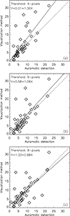 |
Fig. A.1. Scatter plots showing correlations of the velocities of the same structure obtained from different methods. In (a), (b), and (c), the threshold describing the neighborhood in which we searched in the following frame for the moving brightening is set to 4 pixels, 6 pixels, and 8 pixels separately. The dashed diagonals show the ideal case of equal velocities from both methods, while the solid lines are the linear fittings. The fitting parameters can be seen in the upper left corner of each panel. |
Another concern is about the determination of the outer boundary of each base brightening. In the first step we chose a threshold of 0.01 based on DoG maps, providing the outlines of the base brightenings. While this method works well to get the location of the base brightening, the outer boundary thus defined takes into account both the enhancement and background. This is the reason why we re-defined the boundary based on the images with the local background removed. We tested the thresholds of 0.65, 0.75 and 0.85 of the maximum intensity within each base brightening based on the background-removed images. Figure A.2 shows the distributions of area and length-to-width ratio when different thresholds are selected. The area of the base brightening, although it changes significantly in value depending on the selection of the threshold, shows consistent distributions that the base brightenings with a relatively smaller area have a higher occurrence frequency. Differently, the selection of the threshold affects the distribution of the length-to-width ratio. With increasing threshold, more base brightenings detected by the visual identification method tend to show a relatively high length-to-width ratio of around 3, which does not correspond with the results from the automatic method. The distribution shows a strong peak at about 2 when the threshold equals 0.65 of the maximum. Also note that when the threshold goes down to 0.65 of maximum, the 2-dimensional Gaussian fitting has more difficulty converging, which means the shape of the base brightening is more uneven. In our work, considering all the above factors, a threshold of 0.75-maximum is used for the outlines of base brightenings.
 |
Fig. A.2. Normalized distributions of areas (upper panels) and length-to-width ratio (lower panels) of the base brightenings detected in both methods. The gray bars show results from automatic method and the blue line-filled bars are results from visual identification method for comparison. From left to right panels the boundary threshold are 0.65, 0.75, and 0.85 of maximum. |
Appendix B: HMI extrapolations
We conducted another potential extrapolation test with the data from HMI to compensate for the missing of the active regions in HRT data. This experiment is done for the purpose of proving the effect of the strong magnetic field from the active regions on the directions of nearby open fields. The plumes studied in this work are located in the coronal hole close to ARs NOAA 13105 and NOAA 13107. Unfortunately, due to the separation angle between Earth and Solar Orbiter of more than 90°, no simultaneous observation of these active regions from HMI is obtained. About one week later, the ARs and coronal hole have rotated to reach the disk center region of the sun in the FoV of HMI. However, a new AR NOAA 13127 has emerged during this time very closely to where the plumes were located. To avoid the influence of the newly emerged AR, we finally chose to use the HMI sharp_cea data at 09:00 UT on 28 September 2022, which shows NOAA 13105 and NOAA 13107 in the previous rotation when they appear in the western hemisphere in HMI FoV as the Sun rotates. Despite that the ARs are stronger and the plumes in our study have not been produced at this point, this dataset could be simply used to study the effect of ARs qualitatively.
To make a comparison, we made two extrapolations. One uses the original data as the bottom boundary and another uses the processed data with the strong magnetic fields (Br above 100 Gauss) from the ARs removed. We did not change the quiet sun and coronal hole regions and some small magnetic concentrations in ARs are left for flux balance. The results can be found in Figure B.1, where the same cross-section parallel to the x − z plane is shown in both extrapolations. The streamlines show the projection of the magnetic field lines on this plane. Compared with panel (b) where there is no ARs, the streamlines on the left side of the plane in panel (a) clearly show a stronger inclination under the effect of ARs.
 |
Fig. B.1. Potential extrapolations with the original HMI data and the processed data with the strong magnetic fields from the ARs removed. One cross section parallel to the x − z plane is selected to demonstrate the directions of magnetic fields. The streamlines show the magnetic field lines projected on this plane. |
All Tables
All Figures
|
Fig. 1. Overview of coronal hole observations. (a) Full-disk image of the Sun provided by Full Sun Imager (FSI) of EUI. The box indicates the region covered by HRIEUV. (b) Image taken by HRIEUV with three boxes showing the base regions of the three plumes shown in panels (c)-(e). Both (a) and (b) are plotted in logarithmic scale in brightness. (c)-(e) Zoom-in normalized images of the base regions of the three plumes. (The associated movie is available online.) |
| In the text | |
|
Fig. 2. Dynamics at the base of plumes. (a) A sample light curve obtained from the base region of plume 2 (see Figure 1(d)). The whole time period (30 min) is divided into four sections (partitioned at orange dashed lines). (b) – (e) Images of the base region of plume 2 acquired at the middle instance from each temporal section in (a). Brightenings identified using chosen thresholds are marked by the contours (colors indicate time progression; as defined by the color bars). The red boxes highlight several examples of the “gradient patterns”, which are formed by contours from successive frames being adjacent to or overlapping one another, thereby illustrating the movement of the brightenings. Note that, even though we have divided the entire observation into four sub-periods, the contour of the brightenings that appears later will inevitably overlap the ones that appear earlier. For example, a discrete contour could be either a brightening that only appears in one frame, or a brightening that does not show a significant movement. |
| In the text | |
|
Fig. 3. Zoom into the plume bases observed on October 13, 2022 17:10 UT. The intensity-weighted center of each base brightening along the evolution is overplotted on the images. The color represents the time of the first appearance of each base brightening (see the color bar). |
| In the text | |
|
Fig. 4. Distributions of the properties of the base brightenings selected with the visual identification method (50 base brightenings). (a) shows the mean intensity of the base brightenings without subtracting the local background while (b) shows the mean intensity with the local background removed. (c) – (f) show the lifetime, area, length-to-width ratio, and velocity. The velocity here is a projection on the PoS and is calculated using the first and last positions of the intensity-weighted center of the base brightening. |
| In the text | |
|
Fig. 5. Normalized distributions of the properties (mean intensity, lifetime, area, length-to-width ratio, and velocity) of the base brightenings detected with both visual identification method (50 base brightenings) and automatic method (451 base brightenings). The gray bars show the results from the automatic method and the blue line-filled bars show the results from the visual identification method. |
| In the text | |
|
Fig. 6. (a) HRIEUV image of plume 2 showing the base region and plume streams. The overplotted box shows the position of the slice that is taken to form the time-slice plot shown in (b). (b) Time-slice plot. The PDs are marked with blue dashed lines. The average velocity is 112 km s−1. The red arrow points to one of the PDs, which is potentially transformed by a slow-moving base brightening. As an example, (c) shows the light curves at different distances (see different colors) of the first PD. The light curves are fitted with a Gaussian function. The central time (where the light curve peaks) derived from the fitting can be found in (d), together with the linear fitting of distances vs. central time. The error of intensity in (c) is calculated taking the readout noise and dark current into account. This error is propagated to get the error of central time in (d). (The associated movie is available online.) |
| In the text | |
|
Fig. 7. Magnetic field imprints of the plumes. (a) Field of view covered by both HRIEUV and HRT data. The background image comes from the HRIEUV at 17:00 UT. The red (blue) contours of LoS magnetic field with the level of positive (negative) 50 gauss are overplotted. (b), (d) and (f) show the extrapolated magnetic field lines at the location of the three plumes, the sub-regions marked with boxes in (a), (c), (e), and (g) are histograms of frequency of the separation angle between the local magnetic field vector and LoS of three plumes. This separation angle is obtained as an average over all pixels at heights between 2000 and 4000 km along each field line; see the yellow boxes in (b), (d), and (f). |
| In the text | |
|
Fig. 8. Propagating disturbances. (a) HRIEUV image of plume 2. Positions at different distances from the base region are marked with diamonds. The intensities along the slits perpendicular to the stream direction at these positions are fitted by a Gaussian function. (b) and (c) show the peak and FWHM of the fitted Gaussian functions, as a function of the distance along the PD, at three instances (each separated by 20 s; as identified with different colors). Same as Figure 6c and d, the error of intensity in (b) comes from the detector readout noise and dark current and the error of width is derived from the Gaussian fitting. |
| In the text | |
|
Fig. A.1. Scatter plots showing correlations of the velocities of the same structure obtained from different methods. In (a), (b), and (c), the threshold describing the neighborhood in which we searched in the following frame for the moving brightening is set to 4 pixels, 6 pixels, and 8 pixels separately. The dashed diagonals show the ideal case of equal velocities from both methods, while the solid lines are the linear fittings. The fitting parameters can be seen in the upper left corner of each panel. |
| In the text | |
|
Fig. A.2. Normalized distributions of areas (upper panels) and length-to-width ratio (lower panels) of the base brightenings detected in both methods. The gray bars show results from automatic method and the blue line-filled bars are results from visual identification method for comparison. From left to right panels the boundary threshold are 0.65, 0.75, and 0.85 of maximum. |
| In the text | |
|
Fig. B.1. Potential extrapolations with the original HMI data and the processed data with the strong magnetic fields from the ARs removed. One cross section parallel to the x − z plane is selected to demonstrate the directions of magnetic fields. The streamlines show the magnetic field lines projected on this plane. |
| In the text | |
Current usage metrics show cumulative count of Article Views (full-text article views including HTML views, PDF and ePub downloads, according to the available data) and Abstracts Views on Vision4Press platform.
Data correspond to usage on the plateform after 2015. The current usage metrics is available 48-96 hours after online publication and is updated daily on week days.
Initial download of the metrics may take a while.