| Issue |
A&A
Volume 708, April 2026
|
|
|---|---|---|
| Article Number | A245 | |
| Number of page(s) | 23 | |
| Section | Interstellar and circumstellar matter | |
| DOI | https://doi.org/10.1051/0004-6361/202557351 | |
| Published online | 09 April 2026 | |
Contribution of neutral gas to Faraday tomographic data at low frequencies
A first extensive comparison between real and synthetic data
1
Laboratoire de Physique de l’École normale supérieure, ENS, Université PSL, CNRS, Sorbonne Université, Université Paris Cité, Observatoire de Paris,
F-75005
Paris,
France
2
INAF – Osservatorio Astrofisico di Arcetri,
Largo E. Fermi 5,
50125
Firenze,
Italy
3
AIM, CEA, CNRS, Université Paris-Saclay, Université Paris Cité,
91191
Gif-sur-Yvette,
France
★ Corresponding author: This email address is being protected from spambots. You need JavaScript enabled to view it.
Received:
22
September
2025
Accepted:
22
January
2026
Abstract
Context. The LOFAR observations of diffuse interstellar polarization at meter wavelengths reveal intricate polarized-intensity structures with an unexpected correlation with neutral H i filaments that cannot be reproduced in simulations with a low cold-neutral-medium (CNM) abundance.
Aims. We aim to investigate whether magneto-hydrodynamic simulations of a thermally bi-stable neutral interstellar medium, with a range of CNM mass fraction, can reproduce the properties of the 3C196 field, whicH is the high-Galactic-latitude test observational field.
Methods. Using 50 pc simulations with varying levels of turbulence and compressibility, we generated synthetic 21 cm and synchrotron observations, including instrumental noise and beam effects, for different line-of-sight orientations relative to the magnetic field. To this end, we developed the code Mock Observation Of Synchrotron Emission (MOOSE) used to generate synthetic synchrotron polarization and Faraday tomography. We also developed a metric, η, based on the histogram of oriented gradients (HOG) algorithm, to quantify the relative contribution of cold and warm neutral medium structures to the Faraday tomographic data.
Results. The synthetic observations show levels of polarization intensity and rotation measure values comparable to those of the 3C196 field, indicating that thermal electrons associated with the neutral H i phase can account for a significant fraction of the synchrotron polarized emission at 100–200 MHz. The simulations consistently reveal a correlation between CNM and Faraday tomographic structures that depends on turbulence level, magnetic-field orientation, and observational noise, but only weakly on CNM mass fraction. We found slightly weaker correlation level between the CNM and polarized-synchrotron emission than that observed in the 3C196 field. Many elements could contribute to this result: the ne prescription, contribution of the warm ionized medium (not modeled), the longer line of sight (LOS) in the data compared to the simulations, and the Fourier driving producing CNM structures that are less aligned with B.
Conclusions. These results, although based on comparison with the 3C196 field alone, suggest that low-frequency polarimetric observations provide a valuable probe of magnetic-field morphology in the multiphase interstellar medium of the solar-neighborhood, while simultaneously underscoring the need for improved modeling of the turbulent, multiphase, and partially ionized interstellar medium. A broader comparative analysis will be essential to more fully clarifying how our findings inform the connection between low-frequency polarization data and the structure of partially ionized gas.
Key words: methods: numerical / methods: statistical / ISM: clouds / cosmic rays / ISM: magnetic fields / ISM: structure
Publisher note: Figure 4 was not correctly reproduced: the blue-violin mark was missing. It was corrected on 13 May 2026.
© The Authors 2026
 Open Access article, published by EDP Sciences, under the terms of the Creative Commons Attribution License (https://creativecommons.org/licenses/by/4.0), which permits unrestricted use, distribution, and reproduction in any medium, provided the original work is properly cited.
This article is published in open access under the Subscribe to Open model. This email address is being protected from spambots. You need JavaScript enabled to view it. to support open access publication.
1 Introduction
The transition from the warm neutral medium (WNM) to the cold neutral medium (CNM) is a critical step in the interstellar medium (ISM) cycle, and pivotal for the formation of molecular clouds and stars. This transition, largely governed by the thermal instability (e.g., Field 1965; Wolfire et al. 2003; Audit & Hennebelle 2005; Saury et al. 2014; Godard et al. 2024), marks a key stage in the condensation of diffuse gas into denser, star-forming regions. Despite extensive theoretical and numerical investigations, the precise mechanisms regulating this phase change remain incompletely understood. Among the factors influencing this transition, magnetic fields have emerged as a possible player.
The polarization of thermal dust emission, whicH is extensively mapped by the Planck satellite (Planck Collaboration Int. XXXII 2016), has offered high-resolution insights into the magnetic-field morphology, particularly in relation to filamentary structures in the diffuse ISM. These studies revealed statistical alignments between magnetic fields and H i filaments, suggesting a strong coupling between magnetic-field orientations and the physical processes governing the ISM. Magnetic fields in the ISM have been increasingly recognized as a key factor in shaping its structure and dynamics, particularly through their interaction with neutral gas phases. Recent work by Clark et al. (2015) and Clark & Hensley (2019) used H i observations and Planck dust-polarization data to reveal alignment between the morphology of H i filaments and the orientation of magnetic fields. These studies provided evidence that filamentary structures in the CNM may trace the structure of the local magnetic field.
While starlight and dust-polarization studies have advanced our understanding of the magnetic field’s large-scale morphology, another proxy of the magnetic field has been less studied for the local ISM. Synchrotron emission, arising from relativistic electrons spiraling along magnetic-field lines, provides a complementary perspective. Synchrotron radiation traces the component of the magnetic-field perpendicular to the line of sight (LOS), offering insights into its strength and orientation (Rybicki & Lightman 1979; Longair 2011; Padovani et al. 2021). Observations at low radio frequencies are particularly valuable, as they capture Faraday rotation effects, wherein the plane of polarized light rotates as it propagates through a magnetized, ionized medium (Burn 1966; Sokoloff et al. 1998; Ferrière et al. 2021). This effect depends on the thermal electron density and the magnetic-field component along the LOS, making it a powerful tool for probing the magneto-ionic medium. The degree of rotation experienced by a polarized wave is quantified by the Faraday depth, which depends on the thermal electron density, ne, the magnetic-field component along the LOS, B∥, and s, whicH is the path length.
The technique of Faraday tomography (Brentjens & de Bruyn 2005) exploits these low-frequency radio observations to decompose polarized synchrotron emission by Faraday depth, enabling a non-spatial 3D reconstruction of the magneto-ionic structure of the ISM (Haverkorn & Heitsch 2004; Van Eck 2018; Erceg et al. 2022; Erceg et al. 2024). Recent advancements in radio facilities, such as the Low-Frequency Array (LOFAR; e.g. van Haarlem et al. 2013) have significantly improved the sensitivity and resolution of low-frequency synchrotron-polarization observations, bringing new questions concerning the interplay between magnetic fields and the thermal instability.
A growing body of research seeks to connect these radio observables with neutral gas structures (e.g., Van Eck et al. 2017). Observationally, Bracco et al. (2020) demonstrated that CNM structures, extracted via phase decomposition of 21 cm data with the Regularized Optimization for Hyper-Spectral Analysis (
ROHSA) code (Marchal et al. 2019), exhibit stronger spatial correlations with Faraday tomography data compared to WNM structures. However, numerical simulations by Bracco et al. (2022) reported an inverse trend, with WNM showing greater correlation with synchrotron data. This discrepancy was attributed to the low CNM mass fraction (1 %) in the simulated environment and the absence of instrumental effects in the analysis, highlighting the need for a more systematic investigation. Besides this, depolarization canals, which are narrow regions of reduced polarized intensity observed in LOFAR data (e.g., Jelić et al. 2015; Erceg et al. 2022), have been shown to align with filamentary H i structures in the CNM (Jelić et al. 2018; Clark & Hensley 2019), further supporting a close link between small-scale magnetized structures in the neutral ISM and features seen in polarization observations (e.g., Haverkorn & Heitsch 2004; Jelić et al. 2015). In particular, this behavior was observed in the 3C196 field, which was used in this study for comparison. However, it only represents a single LOS through the Galaxy and therefore cannot fully capture the morphological and physical diversity of the diffuse ISM.
The study presented here revisits these questions using a suite of magneto-hydrodynamic (MHD) simulations (Rashidi et al. 2024) that span a range of CNM mass fractions (10 %–50 %), providing a more representative depiction of the diffuse ISM. In addition, we incorporated a simplified instrument model to simulate telescope beam effects and instrumental noise, ensuring a more realistic comparison between simulations and observations.
To achieve this, we developed a Julia-based (Bezanson et al. 2017) code, Mock Observation Of Synchrotron Emission (
MOOSE), to produce synthetic observations of polarized synchrotron emission from MHD simulations, perform Fara-day tomography, and compute spatial correlations between H i phases and Faraday observables. This approacH is intended to test whether low-frequency synchrotron emission can provide new insights into magnetic-field-driven effects in ISM phase transitions, bridging the gap between theoretical predictions and observational constraints.
The paper is organized as follows. Sect. 2 features a review of the physical properties of the 3C196 field, which was used throughout the analysis for comparison with numerical simulations. In Sect. 3, we present the methods used to analyze the correlation between Faraday tomography observables and neutral gas structures. This includes the histogram of oriented gradients (HOG) method (Soler et al. 2019), the process of generating synthetic synchrotron polarization maps using the
MOOSEcode, and the impact of instrumental effects such as noise filtering and beam convolution. In Sect. 4, we present our findings, focusing on the dependence of the H i-Faraday correlation on CNM fraction, turbulence, and magnetic-field topology. We compare the results of different simulation setups and contrast them with the LOFAR Two-metre Sky Survey (LoTSS) observations of the 3C196 field (Erceg et al. 2022). In Sect. 5, we examine the limitations of our simulations and explore possible physical processes – such as electron-density prescription, cosmic-ray transport, and supernova-driven turbulence – that may influence Faraday tomography observables and their correlation with H i data. Finally, in Sect. 6, we summarize the key findings.
2 The 3C196 field of view
2.1 Observations
The 3C196 field is one of the primary fields of view of the LOFAR epoch-of-reionization key science project. It is located in a diffuse region at high Galactic latitude (l = 171◦ , b = +33◦) centered on the extragalactic source 3C196 (Jelić et al. 2015; Jelić et al. 2018). The angular size of the field is 64 deg2. Observations were carried out between 115 and 189 MHz with 3.2 kHz spectral resolution. It is at the core of the analysis of Bracco et al. (2020), which revealed morphological correlations between low frequencies radio polarization and H i data from the Effelsberg– Bonn H i survey (EBHIS; Kerp et al. 2011; Winkel et al. 2016). In their study, Bracco et al. (2020) used an early single-pointing version of the 3C196 field LOFAR observations, which shows a sharp increase in noise at the edges of the field of view. Later on, Erceg et al. (2022) presented a complete Faraday tomographic mosaic of the LoTSS survey conducted with the LOFAR telescope, whicH includes the 3C196 field. Observations were conducted between 120 and 168 MHz with a resolution of 97.6 kHz. The mosaicking strategy, involving overlapping fields of view, results in a more uniform noise level across the observed area.
In this work, we reproduced the data-analysis methodology of Bracco et al. (2020). To do so, we used the LOFAR data product of Erceg et al. (2022) and, as Bracco et al. (2020), the 21 cm data from EBHIS. The data products have a respective angular resolution of 4′ for LOFAR and 10′8 for EBHIS. To compare the two datasets, the LOFAR polarimetric data cubes were convolved at the EBHIS resolution and then projected onto the EBHIS grid.
2.2 Physical properties of the 3C196 field
In this section, we describe the general physical properties of the 3C196 field, which we compared to the simulations. We are mostly interested in the multiscale properties of the H i data and the intensity of the magnetic field.
Based on EBHIS 21 cm data (Winkel et al. 2016), the average H i column density in the 3C196 field is NH i = 4.2 × 1020 cm−2. The H i phase decomposition done in Bracco et al. (2020) using
ROHSA(Marchal et al. 2019) indicates a WNM column density of NWNM = 2.4 × 1020 cm−2. The fraction of the H i in the CNM phase, defined as fCNM = NCNM/NH i, is 38%.
The
ROHSAdecomposition also allows us to estimate the H i velocity dispersion along the LOS. Here, we took the WNM as the reference as it is volume-filling. The WNM velocity dispersion σu in the 3C196 field is 16.3 km s−1. This velocity dispersion results from the combination of thermal and turbulent contributions and can be expressed as
 . Assuming a reference temperature of 7000 K for the WNM, the thermal velocity dispersion is σtherm ≈ 7.6 km s−1, leading to a turbulent velocity dispersion of σturb ≈ 14.4 km s−1. Following Kolmogorov (1941), the turbulent velocity dispersion is related to scale l as
 (1)
(1)
where σu,1 pc is the 1D turbulent velocity dispersion along the LOS at a scale of 1 pc.
According to the 3D-dust map of Edenhofer et al. (2024), the Galactic interstellar matter observed in the 3C196 field is distributed over a depth of ∼350 pc and located approximately 200 pc from the Sun, corresponding to the wall of the Local Bubble. Assuming the WNM is filling the whole depth of 350 pc, we obtain σu,1 pc = 2.0 km s−1. At the 50 pc scale (the simulation scale), the extrapolated 1D velocity dispersion is σu,50 pc = 7.4 kms−1, yielding a 3D turbulent velocity dispersion of σ3D = 12.8 km s−1.
Moments 0, 1, and 2 of the Faraday spectra of the 3C196 field are displayed in Fig. 1. Previous analyses of this region (Jelić et al. 2015; Turić et al. 2021; Erceg et al. 2022) indicate that the magnetic field is largely dominated by its plane-of-the-sky component, with only a modest contribution along the LOS. Therefore, the observed Faraday depths do not necessarily imply locally enhanced LOS magnetic-field strengths, but rather result from the interplay of electron density and path length along this particular LOS. According to Heiles & Troland (2005), the magnetic-field strength at high Galactic latitude is estimated as 6 ± 2 µG based on 21 cm Zeeman-splitting measurements.
3 Methods
3.1 Description of numerical simulations
In this study, we used ideal-MHD simulations designed with the
RAMSEScode (Teyssier 2002; Fromang et al. 2006), which uses adaptive mesh refinement (AMR) up to 10243. We used a version of these simulations computed on a Cartesian grid of 2563 pixels. The box’s physical size is L = 50 pc aside, leading to a resolution of ∆x ≈ 0.20 pc.
The physical conditions we want to reproduce are the ones of atomic gas clouds or those transitioning to molecular gas as expected on the walls of the Local Bubble (Inoue & Inutsuka 2016). In this diffuse medium (0.1 to 100 cm−3, Ferrière (2001)), the self-gravity energy density is significantly lower (two-to-three orders of magnitude) than turbulent and magnetic energy densities; hence, self-gravity is excluded from the simulations. The cooling function is based on Audit & Hennebelle (2005) and closely follows Wolfire et al. (2003). It includes photo-electric heating of dust grains and cooling by electron recombination onto dust grains, as well as collisional excitation of Ly α, C II, and OI emissions.
To maintain turbulence in the simulation, a Fourier space forcing was modeled using an Ornstein–Ulhenbeck stochastic process (Eswaran & Pope 1988; Saury et al. 2014). A turbulent velocity field was added on a large scale (1 < k < 3), peaking at k = 2 (half the box size, L). The forcing was parametrized by its amplitude, Af,RMS, and the compressive-to-solenoidal mode decomposition parameter, χ, where χ = 0 only contains solenoidal modes and χ = 1 only compressible modes.
In this study, we used the set of 14 simulations described in Table 1. The mean B-field intensity of all simulations is 7.64 µG. The ratio of compressible to solenoidal modes of the forcing was varied from χ = 0 to χ = 1, and its amplitude, Af,RMS, was varied between 9000 and 72 000, producing 3D velocity dispersions from 4.3 to 14.5 km s−1.
Each simulation began with WNM conditions in place, a density of nH = 1 cm−3, and a temperature of T = 8000 K. The magnetic field was initiated uniformly along the x-axis, which gives a prevailing direction for the B field in the simulation box; ∇ · B = 0 was guaranteed by the use of the constrained transport method. Due to the nature of the periodic box, the coherence of the magnetic field along the x-axis was maintained at each time step.
As the simulations evolve, shear flows and shock waves emerge in the volume, causing local pressure variations in the WNM leading to the formation of CNM structures. We let simulations proceed until a steady state was achieved when velocity dispersion, gas-phase mass fractions, density, and temperature PDFs reached a stationary state, within at least three dynamical timescales, tdyn = L/σu,3D, where σu,3D is the velocity dispersion in 3D. An illustration of one simulation is given in Fig. 2, where two slices of the density field are shown, one along and one perpendicular to the mean magnetic field, represented here using the line integral convolution (LIC) technique (Cabral & Leedom 1993).
For each simulation, we decomposed the gas in the three main H i components: CNM, lukewarm neutral medium (LNM), and WNM. As in Saury et al. (2014), we notice that CNM structures form preferentially in over-pressured and less turbulent WNM regions. The overall CNM mass fraction in our set of simulations tends to increase with the rate of compressible modes, and even more so for less turbulent ones. This is illustrated in Fig. 3, where the CNM mass fraction is plotted for the last time step of each simulation. Table 1 also provides the CNM mass and volume fractions for the last time step of each simulation, together with the root-mean-squared (RMS) values for BRMS, uRMS, and the velocity dispersion, σu,1pc, of the gas at 1 pc.
In this paper, we regularly refer to simulation 7, which we used as our case study throughout our analysis. This simulation has a CNM fraction of 29% and σu,1pc = 1.1 km s−1, both of which are slightly lower than the values of the 3C196 field, but still representative of the diffuse ISM. Moreover, the Fara-day depth distributions of the simulations and of the 3C196 field, shown in Fig. 4, exhibit comparable orders of magnitude, namely a few rad m−2.
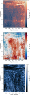 |
Fig. 1 Moment 0 (integrated polarized intensity) de-biased for noise (top), Moment 1 (middle) and Moment 2 (bottom) of the 3C196 field from LOFAR LoTSS DR2 Faraday tomographic data (Erceg et al. 2022). |
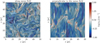 |
Fig. 2 Slice through the simulation cube showing the logarithmic gas density overlaid with magnetic-field orientation using the line integral convolution (LIC) technique. Left: projection along the mean magnetic-field direction. Right: projection perpendicular to the mean field. |
Description of simulations used in this study.
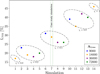 |
Fig. 3 CNM mass fraction, fCNM, of the different simulations used in this study. The dashed circles highlight the simulations with the same turbulent mode ratio, χ. Colors show the initial input for the forcing amplitude. |
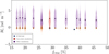 |
Fig. 4 M1 distributions as a function of fCNM for the set of simulations. These distributions are measured along two orthogonal directions: parallel (lighter color) and perpendicular (darker color) to the mean magnetic field. Filled circles indicate the corresponding mean values ⟨M1⟩, outlined in black. The case-study simulation is highlighted in red, while the remaining simulations are shown in violet. Two simulations have fCNM = 26%, leading to an overplotting of their respective distributions. The 3C196 field is displayed in blue witH its associated distribution and mean value. |
3.2 Synthetic observations
In order to reproduce the analysis of Bracco et al. (2020), which compared polarized synchrotron and 21 cm emission data of the 3C196 field, we had to create corresponding synthetic observations for each numerical simulation. This section describes how these were created, including the effects of Faraday rotation andthe LOFAR beam on the polarized synchrotron emission.
3.2.1 Synchrotron emission
In order to produce synthetic observations of synchrotron emission and its polarization, whicH is the basis of the Faraday tomography, we used Eqs. (1)–(9) of Padovani et al. (2021) derived from Ginzburg & Syrovatskii (1965). As cosmic-ray electrons (CRe) travel through the ISM, they lose energy due to interactions with matter, magnetic fields, and radiation (Longair 2011). These interactions modify the cosmic-ray energy spectrum, je(E), where E represents the CRe energy.
For the CRe energy spectrum, je(E), we used the same power-law definition as in Padovani & Galli (2018) and Orlando (2018):
 (2)
(2)
where j0 = 2.1 × 10¹⁸ eV−1s−1cm−2sr−1, E0 = 710 MeV, a = −1.3, and b = 1.9. In our case, je(E) was considered spatially constant in the simulated box.
Noting me as the electron mass, e the electron charge, and c the speed of light, the synchrotron-specific emissivity at a position, s, can be divided into two linearly polarized components: one parallel and one perpendicular to the magnetic-field component orthogonal to the LOS, B⊥:
 (3)
(3)
and
 (4)
(4)
where  and νc is defined as the frequency at which the synchrotron intensity of CRe at energy, E, is the greatest:
 (5)
(5)
Synchrotron emission is thus
 (6)
(6)
3.2.2 Faraday rotation
In this paper, we address the scenario where Faraday rotation is completely intertwined with synchrotron emission, leading to differential Faraday rotation (e.g., Sokoloff et al. 1998) as in Bracco et al. (2022). Each layer within the simulated cubes contributes to both synchrotron emission and Faraday rotation.
Stokes Qν and Uν for synchrotron emission are given by the following equations:
 (7)
(7)
and
 (8)
(8)
where Ψloc is the polarization angle at the position s defined as the orientation of B⊥ rotated by 90◦. ∆Ψν describes the Fara-day rotation, whicH is the integral along the LOS between the observer and s. The Faraday rotation depends on the square of the observation wavelength, λ; the electron density, ne; and the magnetic field along the LOS. It is also expressed as
 (9)
(9)
where  and ϕ is the Faraday depth, a quantity independent of wavelength that describes the physical quantities responsible for the angle rotation from the emitting source toward the observer, corresponding to the cumulative Faraday rotation experienced by the polarized emission along the LOS:
![Mathematical equation: ${{\phi (s)} \over {\left[ {{\rm{rad m}}{{\rm{m}}^{ - 2}}} \right]}} = 0.81\mathop \smallint \nolimits_0^s {{{n_e}} \over {\left[ {{\rm{c}}{{\rm{m}}^{ - 3}}} \right]}}{B \over {[\mu {\rm{G}}]}} \cdot {{ds} \over {[{\rm{pc}}]}},$](/articles/aa/full_html/2026/04/aa57351-25/aa57351-25-eq13.png) (10)
(10)
where ds = ∆x in the discrete case of our numerical simulations. From Equations (7) and (8), we define the polarized intensity, P, as
 (11)
(11)
P is commonly computed as an analog of the Fourier transform into the Faraday spectrum:
 (12)
(12)
For the limit case, where the integration is made all along the LOS, i.e., s = 0 and s + ds = L, ϕ becomes the rotation measure (RM).
The Faraday spectrum is represented as a polarized brightness temperature by taking the modulus of F(ϕ), making it a non-negative quantity. Hereafter, we use F(ϕ) as representative of the modulus of Eq. (12).
3.2.3 Electron density
In order to produce synthetic synchrotron observations including Faraday rotation, we needed to estimate the density of thermal electrons, ne, at each position in the cube. The numerical simulations were thus post-processed to estimate ne in units of cm−3 following Eq. (6) of Bracco et al. (2022), which derives the following from Wolfire et al. (2003) and Bellomi et al. (2020):
 (13)
(13)
where ζ16 represents the total ionization rate per hydrogen atom due to energetic photons (including extreme UV and soft X-rays) and CRs expressed in units of 10−16 s−1, T2 is the temperature of the gas expressed in units of 100 K, ϕPAH denotes the recombination rate of electrons onto small dust grains such as polycyclic aromatic hydrocarbons (PAHs). Furthermore,  is the relative abundance of ionized carbon compared to the number of hydrogen atoms (nH). Following Bracco et al. (2022), we used
  and ϕPAH = 0.5, Geff = 1, and ζ = 2.5 × 10⁻¹⁶ s−1 (Padovani et al. 2022) as representative values for the diffuse ISM. The impacts of these choices on our results are discussed in Sect. 5.
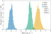 |
Fig. 5 Simulation 7. RM histograms for cubes produced with the LOS parallel, perpendicular, or 45◦ to the mean direction of B. Dashed lines: mean values of the rotation measure maps. The mean values are ⟨RM∥⟩ = 5.5 rad m−2, ⟨RM⊥⟩ = 0.0 rad m−2, and ⟨RM45◦ ⟩ = 3.9 rad m−2. |
3.2.4 Rotation measure
Before computing mock LOFAR observations, it is useful to evaluate the range of Faraday depth that we expect from our simulations. For example, Fig. 5 shows the distributions of RM for simulation 7 (computed using Eq. (10) and integrated over the full LOS) for cubes produced with the perpendicular, parallel, or 45◦ LOS with the mean direction of B. For each orientation, the range of RM values is centered on specific values, illustrating the fact that the strength of B∥ is different in each case. When the LOS is perpendicular to B, the RM values are very close to zero, as expected. For the case where the mean magnetic field is aligned with the LOS, ⟨RM∥⟩ = 5.5 rad m−2. In the intermediate case, where the simulation cubes are produced with a LOS at 45◦ with the mean direction of B, the RM distribution is intermediate, with a mean RM of 4.8 rad m−2. In the three projections, the dispersion of RM is only about 1–2 rad m−2. These RM values fall within the range observed with LOFAR in the 3C196 field (Jelić et al. 2018; Bracco et al. 2020; Erceg et al. 2022). They are also similar to what was reported by Hutschenreuter et al. (2022) in the 3C196 field, with most RM values ranging from −5 to 10 rad m−2. This is interesting as the RM values from Faraday measurements on extragalactic point sources of Hutschenreuter et al. (2022) are probing greater physical depth, as they estimated.
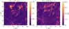 |
Fig. 6 Mock observations for simulation 7 in the case where the LOS is parallel to the mean B field. Left panel: map of Faraday spectrum F(ϕ) at ϕ = 1.75 rad m−2. Right panel: map of 21 cm brightness temperature TB(u) for v = 0.9 km s−1. |
3.2.5 Mock LOFAR observation
In order to compute synchrotron Stokes parameters, we developed a Julia package called
MOOSE1, whicH is described in Appendix A. For each of the 14 simulations, we used the B-field and ne cubes to compute Iν, Qν, and Uν based on Equations (3)–(9).
MOOSEis able to treat any frequency range, but in this work we focused on LoTSS frequencies used for the study of the 3C196-field (Erceg et al. 2022); i.e., ν is in the range of [120, 167] MHz, with a frequency resolution of δν = 98 kHz. As LOFAR interferometric observations are subject to large-scale filtering, we wanted to simulate this effect. To do this, we used a Gaussian kernel, Gker, of standard deviation σLS. We applied a convolution on a given image, Ai,j, as follows:
 (14)
(14)
where  is the image with the large scales are removed.
With Qν and Uν calculated, we computed F(ϕ) using a Julia version of the rotation-measure synthesis (
RM-Synthesis) (Brentjens & de Bruyn 2005) implemented in
MOOSE. Due to the frequency range, which we chose as that of the LoTSS survey (Erceg et al. 2022), the Faraday resolution is 1.14 rad m−2 (see Eq. (61) in Brentjens & de Bruyn 2005). We computed F(ϕ) from ϕ = −10 rad m−2 to 10 rad m−2 with steps of 0.25 rad m−2 to include the range of values of RM found in our simulations (see Fig. 5).
Figure 6 (left) shows an example of polarized intensity at a specific Faraday depth, F(ϕ), for simulation 7 in the case where the mean B field is along the LOS. For all our simulations, F(ϕ) displays complex structures that reflect the interplay between the electron density and magnetic-field morphologies.
3.2.6 Mock 21 cm line observation
To simulate 21 cm line observations of neutral hydrogen, we computed the brightness temperature, TB(u), as a function of velocity, u, along each LOS using the following radiative transfer equation:
 (15)
(15)
Here, the l index runs over the cells along the LOS, τ(l, u) is the 21 cm optical depth at position l and velocity u, and T(l) is the gas temperature (taken as a proxy for the spin temperature). In this formulation, the term  represents the emission from cell l and velocity u, while the exponential factor exp
  describes the attenuation of this emission by the gas located between position k and the observer.
We assumed that the opacity τ(l, u) is
 (16)
(16)
where C = 1.82243 × 1018 cm−2 K−1 (km/s)−1 and NH(k, u) is the column density in cell l expressed as a Gaussian with thermal broadening centered on the local velocity, u = v(l); and normalized by the local density, nH(l):
 (17)
(17)
with
 (18)
(18)
In theory, ∆ should also include the turbulent velocity dispersion at scales smaller than the cell scale. We made this simplification as the typical turbulent velocity dispersion at the scale of a cell (0.2 pc) is ∼0.6 km s−1, assuming a typical value of σu,1pc = 1 km s−1 and using Eq. (1). This would become significant only for gas at T < 45 K, whicH is very rare in the simulations used here.
We produced synthetic 21 cm observations for each simulation using this formalism. An example of a 21 cm channel map is shown in Fig. 6, right. As for F(ϕ), the 21 cm channel maps show a complex multiscale structure with several narrow and twisty filaments. On the other hand, contrary to F(ϕ), where the structure is very different depending on the orientation of B with respect to the LOS, the structure in TB(u) is morphologically very similar in all directions.
3.2.7 H i phases cubes
Bracco et al. (2020) used
ROHSAto decompose the EBHIS 21 cm observation of the 3C196 field into phases of the neutral hydrogen. They defined the CNM as Gaussian components with σ ≤ 3 km s−1, and the WNM with components with σ ≥ 6 km s−1. The LNM is everything in between. To avoid having to run
ROHSAon every 21 cm synthetic observation of our simulation set, we chose to segment the H i phases based on the 3D temperature field directly. Assuming a Mach number of 1 and 2 for the WNM and CNM, respectively (Marchal et al. 2024; Heiles & Troland 2003), these σu thresholds correspond to the following temperature ranges: TCNM ≤ 500 K, 500 < TLNM < 3500 K, and TWNM ≥ 3500 K.
In practice, for a given phase (CNM, LNM, WNM) we identified the voxels in 3D corresponding to its temperature range; then, we produced 21 cm synthetic observations using only those voxels. Therefore, for each simulation setup we produced four 21 cm cubes for the total, H i, CNM, LNM, and WNM.
4 Results
4.1 Global properties of TB(u) and F(ϕ)
The H i and Faraday structures of simulation 7 are illustrated in Figures 7 and 8 with views parallel and perpendicular to the mean B field. On the left, these figures show the column-density maps of the H i components (total, CNM, and WNM) highlighting the striking filaments of the CNM as well as the diffuse structure of the more volume filling WNM. On the right, we show the moments (M0, M1, and M2) of the Faraday cube; see Appendix B. These can be directly compared to the moments of the 3C196-field LoTSS observations (Fig. 1).
The Faraday moments of the simulations (Figures 7 and 8) are strongly influenced by the orientation of the magnetic field. In the case perpendicular to the mean field, the values of M1 remain close to zero due to the weak field component along the LOS. On the other hand, when the magnetic field is parallel to the LOS we observe values of M1 that are consistently positive and fall within the positive range observed in the M1 map of Erceg et al. (2022).
Regarding the spread of the Faraday spectra estimated using M2, the values are very small in the case where B is perpendicular to the LOS, very close to theoretical RMSF of LoTSS, whicH is 1.03 ∼ rad m−2 estimated for the theoretical RMSF of LoTSS. On the other hand, the case where B is parallel to the LOS shows M2 values comparable to the ones estimated in the LoTSS 3C196 field.
The histograms of the first-order moment M1 are shown in Fig. 9 (top panel). For the 3C196 field, M1 has a mean value of approximately 0.2 rad m−2 and a standard deviation of 0.9 rad m−2. Among the simulations, the perpendicular case provides the closest matcH in terms of mean value, which reaches ⟨M1⟩ = −0.2 rad m−2, while the parallel and 45◦ cases have ⟨M1⟩ = 2.4 rad m−2 and ⟨M1⟩ = 1.7 rad m−2, respectively.
The Faraday spread M2 (de-biased from noise) measured in the 3C196 field has a median value of approximately 1.7 rad m−2 (see right panel of Fig. 9). Observed values, even after de-biasing from noise, are generally slightly higher than what was recovered in the synthetic observations constructed without noise. The best agreement was found when the emission was integrated along the direction rotated by 45◦ to the mean magnetic field, yielding a mean of ⟨M2⟩ = 1.5 rad m−2. This is close to the the case where B is parallel to the LOS (⟨M2⟩ = 1.4 rad m−2), but with a narrower distribution. The perpendicular configuration shows lower values, as expected because the B component along this direction is very low, with ⟨M2⟩ = 1.0 rad m−2.
One striking feature of the LoTSS polarization data shown in Erceg et al. (2022) is the presence of long and thin depolarization canals; i.e., filamentary regions with the maximum F(ϕ), Pmax, close to zero (for more details, see Sokoloff et al. 1998; Haverkorn & Heitsch 2004). Maps of Pmax (LOS perpendicular and parallel to B) are shown in Fig. 10. Structures with almost zero intensity are seen in the simulations, especially in the case where the mean B field is aligned with the LOS. However, the long, straight canals detected in the LoTSS survey are not reproduced.
4.2 Correlation between LoTSS and EBHIS data
Following the same methodology of Bracco et al. (2022), we compared cubes of H i brightness temperature with Faraday cubes using the HOG method (Soler et al. 2019). The core principle of HOG is to measure the morphological alignment between two images, Ai,j and Bi,j, where i and j denote the image coordinates. It relies on the assumption that the local appearance and shape of an image can be fully characterized by the distribution of its local intensity gradients or edge directions. From this assumption, the gradients of the two images can be computed using Gaussian derivatives, yielding ∇Ai,j and ∇Bi,j. Following the definition in Soler et al. (2019), the angle between the two gradient vectors, α, can then be determined as follows:
 (19)
(19)
where  is the unit vector perpendicular to the plane of sky. HOG tests whether the distribution of angle, α, is uniformly distributed or has a preferential alignment at α = 0, using the projected Rayleigh statistics defined as
 (20)
(20)
where ωi,j is the statistical weight corresponding to each αi,j. The Rayleigh statistics parameter, V, is thus the estimate of how well the two images are morphologically correlated. For more details about this technique, see Soler et al. (2019).
The observational maps do not have the same dimensions as those from the simulations. To address this, we introduced a normalization factor, Vmax, defined as the maximum value of V. The maximum of V is attained when the gradients of the two maps are perfectly aligned (i.e., αi,j = 0) and supposing the weights are all the same (i.e., ωi,j = ω) (also detailed in Mininni et al. 2025). From Eq. (20), this yields Vmax = (2N)1/2.
Specifically, let Fi,j,ϕ represent the Faraday cube and  the 21 cm brightness temperature cube, where i, j are pixel indices on the plane of the sky. For each pair (ϕ, u), we applied HOG using a local kernel around Fi,j and
  . This allowed us to construct maps parameterized by (ϕ, u), illustrating the spatial correlation between specific F(ϕ) and corresponding Tb(u).
The correlation in the 3C196 field reported in Bracco et al. (2020) has since been updated using LoTSS data and the same phase decomposition of the EBHIS data done with
ROHSA. In Fig. 11, the ratio
 is represented on a map with axes ϕ and vLSR. In the H i 21 cm data, two distinct velocity regions can be identified: one around vLSR = 0 km s−1 and another around vLSR = 20 km s−1, similar to the findings of Bracco et al. (2020). Along the ϕ-axis, a broad structure is observed, spanning approximately 5 rad m−2, with a central peak around ϕ = 0 rad m−2.
This structure appears bright across all velocities in H i and WNM. For the CNM, velocities extend from vLSR = −10 km s−1 to vLSR = 20 km s−1, with a strong correlation at 20 km s−1. In contrast, for the LNM phase, this structure spans a more limited velocity range, from vLSR = −20 km s−1 to vLSR = 0 km s−1.
The highest value is  , but as the maximum is sensitive to outliers, we show the 98th percentile of
  ,
,  for each ϕ in the lower panels of Fig. 11. Based on this HOG metric, the strongest correlation between TB(u) and F(ϕ) is found for the CNM (also seen in the total H i) compared with the WNM and LNM components. This is compatible with the results of Bracco et al. (2020).
In order to further quantify the level of correlation of the CNM and WNM phases, we used the maximum of  for each phase and computed the following ratio:
 (21)
(21)
This value reflects the strength of the dominant correlation among the two: η < 1 is indicative of a stronger correlation of the Faraday data with the CNM, while η > 1 shows a stronger correlation with the WNM. In the 3C196 field of view, we find η = 0.73, which supports the visual observation in Fig. 11 that the CNM exhibits the strongest correlation with the Faraday data.
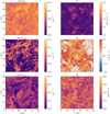 |
Fig. 7 Column density (left panels) and Faraday moment maps (right panels) for case-study simulation, witH integration along the mean magnetic field. Top to bottom: logarithmic column-density maps of total H i, CNM, and WNM; moments 0, 1, and 2 of the Faraday spectrum. |
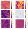 |
Fig. 8 Same as Fig. 7, but for the case where the LOS is perpendicular to the mean magnetic field. Due to the weak LOS magnetic component, M1 values remain close to zero and M2 is narrower across the field. While the density structures of CNM and WNM are similar to the parallel case, the Faraday moments show significantly reduced signal, consistent with expectations for a transverse magnetic-field configuration. |
4.3 Correlation between Faraday tomography and H i emission with numerical simulations
We applied the same HOG methodology to the synthetic observations of our simulation set. Figures 12 and 13 present the HOG results for the correlation of the H i phases with the Fara-day cube for simulation 7 for two orientations (mean B parallel and perpendicular to the LOS). For both orientations the WNM and LNM exhibit higher correlation with Faraday structures than the CNM, in contrast with the results for the 3C196 field of view.
For the case where the mean B field is aligned with the LOS (Fig. 12), the WNM and LNM have  values peaking at 0.12. The CNM, although less correlated, reaches values (
 ) very close to the maximum
  observed in the 3C196 field. The curve of
  confirms this trend, with the WNM displaying the broadest and strongest peak, followed by the LNM and CNM. The strongest correlation is observed around ϕ ≈ 3 rad m−2, whicH is consistent with the expected Faraday depth range for a magnetic field aligned with the LOS.
For the case where the magnetic field lies in the plane of the sky (Fig. 13), the values of  are similar, but the structure in the map of
  is much narrower in ϕ space compared to the case B parallel to the LOS. The WNM and LNM still exhibit the highest correlation, but here the CNM correlation is even lower. In this configuration, the correlation is concentrated near ϕ ≈ 0 rad m−2, whicH is expected since a predominantly perpendicular field results in minimal Faraday rotation.
Overall, the case-study simulation produces  values of total H i, WNM, and LNM that are approximately twice as high as those observed in the 3C196 field. The CNM phase has
  values lower than the other phases, but they reach levels consistent with observational values (
 ).
).
Interestingly, for the case where B is perpendicular to the LOS (Fig. 13), the total H i displays a  curve with a distinctive double-peaked, U-shaped profile. As shown in Fig. 2, right, in this orientation some dense structures associated with the CNM appear misaligned or even orthogonal to the projected B field. This morphological decoupling reduces the coherence between cold H i structures and the Faraday tomographic data. The result is a decrease of
  in velocity channels dominated by CNM emission, inducing this U-shaped form in
  .
.
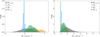 |
Fig. 9 Probability density functions of Faraday spectral moments for the 3C196 field (gray) and for the case-study simulation with three magnetic field orientations: parallel (yellow), perpendicular (blue), and rotated 45◦ (green). Left: first-order moment, M1, showing higher values in the parallel case and near-zero mean in the perpendicular case. Right: second-order moment, M2, of the Faraday spectrum. |
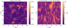 |
Fig. 10 Maximum polarized-intensity maps (Pmax) from the case-study simulation, illustrating the presence and morphology of depolarization canals. Left: integration along the LOS parallel to the mean magnetic field. Right: integration perpendicular to the mean field. Linear, canal-like features are prominent in the parallel case, while more circular structures dominate in the perpendicular configuration. |
4.4 Noise effects on HOG results
To assess the impact of noise on the correlation between the H i phases and the Faraday structures, we added white noise to the mock H i and Faraday data. For H i, noise was added to each velocity channel at various levels with respect to the σEBHIS = 90 mK noise (Winkel et al. 2016): σEBHIS/5, σEBHIS/2, σEBHIS, 2 × σEBHIS, and 10 × σEBHIS. For Faraday, the noise was added to Qν and Uν, with a noise amplitude tuned to reproduce specific S/Ns in Faraday depth space, including the S/N of the observational data – whicH is five – as well as both lower and higher S/N regimes.
As shown in Fig. 14, the addition of noise to the H i data predominantly affects the WNM structures. Specifically, when increasing the noise level from σEBHIS/5 to 10 × σEBHIS, the maximum correlation value for the CNM decreases by a factor of approximately 1.5, whereas for the WNM, the corresponding decrease reaches a factor of 2.5.
Two effects are at play here. First, the WNM has a broad emission line due to its larger thermal broadening. Therefore, a given column density of WNM is more spread out in velocity with lower values of TB(u) than the same column density of CNM that will be narrow and brighter. Second, the WNM has an intrinsic diffuseness and lower spatial contrast compared to the CNM, which forms narrow, high-contrast filaments. As a result, the WNM large-scale structures with smoother gradients are more easily suppressed by noise, particularly at high spatial frequencies where gradient-based methods such as HOG are most sensitive.
Contrary to TB(u), adding noise to Qν and Uν affects both the WNM and CNM in a similar manner. As shown in Fig. 15, increasing the S/N in the Faraday space (S/Nϕ) from two to six leads to an increase in the maximum correlation value by a factor of approximately 1.5 for both phases. In the case where the signal amplitude equals that of the noise (i.e., S/Nϕ = 1), the resulting correlation between the Faraday cube and the H i data is effectively random ( ), as expected. The case perpendicular to the mean field gives similar results.
In conclusion, noise in TB(u) tends to decrease η (i.e., the noise decreases the correlation of WNM compared to CNM), while noise in F(ϕ) does not affect η as it reduces the absolute value of  for all phases.
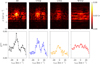 |
Fig. 11 HOG |


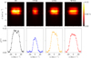 |
Fig. 12 HOG |


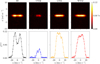 |
Fig. 13 HOG |

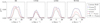 |
Fig. 14 Effect of increasing noise in H i data on the HOG correlation with Faraday tomography structures for the case-study simulation along the mean field. Each panel displays the 98th percentile of the normalized Rayleigh statistic |

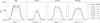 |
Fig. 15 Impact of increasing noise in the Faraday data on the HOG correlation between phase-separated H i structures and Faraday depth features for the case-study simulation along the mean field Each panel shows the 98th percentile of the normalized Rayleigh statistic ( |

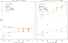 |
Fig. 16 Dependence of HOG correlation maxima ratio, η, on the derivative kernel size used in the gradient computation for different levels of Gaussian noise added to the H i data. Left: case-study simulation with the magnetic field aligned with the LOS. Right: same simulation, but with the mean field perpendicular to the LOS. The observational value from the 3C196 field is shown for comparison (dashed line). |
4.5 Kernel size effect on HOG results
An important parameter of the HOG method is the derivative kernel size, σHOG, that dictates the scale over which the spatial gradient is calculated. This parameter might have a different effect on  for the WNM and CNM as they are not structured at the same scale; CNM structures exhibit a more small-scale filamentary morphology, whereas the WNM is present across a broad range of scales with limited small-scale contrast. In this section, we detail how we evaluated the effect of σHOG on η. We did so for different values of the noise level on TB(u) as it has an effect on η (see Sect. 4.4). Figure 16 shows the variation of η as a function of σHOG (in pixels) for different H i noise levels added to simulation 7, for B parallel (left) and perpendicular (right) to the LOS. The observational reference field 3C196 is also shown in this figure for comparison. The values of η for the 3C196 field remain consistently below unity across all kernel sizes, σHOG, indicating that the CNM is systematically more correlated with the Faraday structures than the WNM.
The results on the mock data of simulation 7 show a significant variation of η as a function of σHOG, H i noise level, and orientation of B with respect to the LOS. For case B parallel to the LOS, the value of η is almost independent of σHOG, while η increases significantly with σHOG in the case where B is perpendicular to the LOS. Strong noise in the H i data produces an increase of η with σHOG as the effect of the noise affecting the WNM is gradually reduced. These variations for a single simulation show that observational results on η can depend significantly on the observational conditions (noise level, physical resolution of the observations), but also on the mean orientation of B with respect to the LOS. That said, our analysis shows that the only way to reproduce the values of η seen in the 3C196 field with simulation 7 is to add a high noise level in the H i mock data in order to lower the WNM correlation to the benefit of the CNM. This is discussed further in Sect. 5.
4.6 Variation with physical parameters
4.6.1 Turbulence strength
The HOG analysis described in the previous sections and illustrated in simulation 7 was also performed on our full simulation set. First, in order to understand the nature of the signature observed in Figures 12 and 13, we show the  curves for all simulations in Figures C.1 and C.2. We chose not to apply any instrument model (LOFAR beam, noise on Faraday and H i) to estimate the effect of turbulence level alone.
We observed that simulations with lower turbulence strength have higher  values than simulations with stronger turbulent driving; see Fig. 17. This suggests that lower turbulence, and therefore weaker magnetic fluctuations, enhances the correlation between magneto-ionized observables and the H i phases. However, we also note that η is always higher than what is seen in observational data whatever the turbulence level (i.e., the WNM remains more correlated to F(ϕ) than the CNM). We recall that this experiment was done without any noise in the mock data and, as shown in Fig. 16, noise in the H i data tend to lower η.
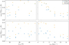 |
Fig. 17 Compilation for all simulations of the maximum value of the 98th percentile of the normalized Rayleigh statistic |


4.6.2 CNM fraction
Finally, one goal of the current study was to evaluate if the fraction of the H i in the CNM phase has an impact on the measured correlation between TB(u) and F(ϕ). To do so, we examined how η varies as a function of fCNM. The aim is to determine whether a higher proportion of CNM in the simulated H i data systematically enhances the correlation with Faraday structures and whether this trend depends on the orientation of the magnetic field with respect to the LOS.
Figure 18 displays η as a function of fCNM and urms. A horizontal dashed line at η = 1 indicates the threshold separating WNM-dominated (η > 1) from CNM-dominated (η < 1) regimes. The value observed in the 3C196 field, ηobs = 0.72, is also shown. In the perpendicular configuration, η reaches high values, particularly for simulations with low CNM fractions – exceeding η = 7 in some cases – whicH indicates a strong WNM–Faraday alignment. As fCNM increases, η decreases but generally remains above one, confirming the persistent dominance of the WNM. In contrast, the parallel configuration shows η values consistently close to or below one across the entire range of CNM fractions with a flat trend. Only at high CNM fractions (fCNM ≳ 35%) does the correlation approach the observational regime where CNM dominates.
To further disentangle the contributions from each phase, the two bottom panels show the respective alignments of WNM and CNM structures with the Faraday map. These panels confirm that the WNM largely dominates the correlation in the perpendicular case, while the CNM only begins to compete in the parallel configuration at high CNM fractions. This suggests that while the presence of CNM is a necessary ingredient for achieving a CNM-dominated regime, it is not the primary driver of the correlation, which depends more critically on the relative orientation of the magnetic field.
In the configuration where the LOS is aligned with the mean magnetic field, the maximum values of  for the CNM and WNM phases follow remarkably similar trends. This suggests that the morphological structures of CNM and WNM are comparable in this case and may both trace the same Faraday structures. In contrast, the perpendicular configuration reveals a clear divergence between the CNM and WNM η values, indicating that their structures differ significantly. As also supported by Fig. 8, this behavior suggests that the WNM structures are more closely aligned with the Faraday morphology, whereas the CNM structures deviate more substantially. This asymmetry highlights the dominant role of the WNM in shaping the observed Faraday features, particularly when the magnetic field lies in the plane of the sky.
5 Discussion
5.1 Well-reproduced observation features
The numerical experiment presented here, representing the multiphase H i post-processed using a classical prescription to estimate the local ionization fraction, is able to reproduce several features seen in observations of the diffuse ISM at high Galactic latitudes. These features are listed below.
The velocity dispersion (σ1pc = 0.7–2.3 km s−1) and CNM fractions (fCNM = 17–46%) are representative of what is measured at 21 cm in the diffuse ISM of the solar neighborhood (Marchal & Miville-Deschênes 2021; Marchal et al. 2024).
The range of F(ϕ) values is comparable to the ones measured with LOFAR in the 3C196 field with an average Faraday depth of −2 < M1 < 3 rad m−2 and spread of the Faraday spectra of M1 ∼ 1–2.5 rad m−2.
The simulations of our experiment produce a range of peak polarization intensity between 0 and 12 K (Figures 10 and D.1). The highest values might not be representative as they were obtained when B is exactly perpendicular to the LOS, but our experiment indicates that such relatively low H i column density (⟨NHI⟩ = 1.55 × 1020 cm−2) can easily produce Pmax values of a few kelvin, similarly to what is observed in the 3C196 field (Pmax ≤ 7 K Jelić et al. 2015).
The synthetic Faraday cubes produced, including the effect of a proxy of the LoTSS uv minimum, show elongated structures with no polarization, reminiscent of the observed depolarization canals (e.g., Erceg et al. 2022).
The HOG analysis used to evaluate the correlation between H i and Faraday structures shows a significant correlation of the CNM features with F(ϕ), as revealed in the 3C196 field (Bracco et al. 2020).
Our results are indicative that the physics implemented in such numerical experiment is capturing fundamental aspects of the physics of the diffuse ISM. Even though these experiments were designed to reproduce the diffuse neutral gas (H i), this study indicates that a simple prescription for computing the ionization fraction (and therefore ne) reproduces several properties of the LOFAR data, including a correlation between CNM structures and the morphology of F(ϕ) maps. We recall that before the results of Van Eck et al. (2017), Jelić et al. (2018), and Bracco et al. (2020), the RM values and Faraday structures observed in low-frequency radio data were thought to originate mostly from thermal electrons located in the warm ionized medium (WIM). Our numerical study indicates that even witH its low ionization fraction (∼10−2 in the WNM and ∼10−4 in the CNM), the H i gas contributes significantly to the Faraday rotation signal, at levels strong enough to capture a correlation between F(ϕ) and the CNM 21 cm emission. This is compatible with the results of Boulanger et al. (2024) which, through a totally different approach based on UV-absorption data, also concluded that electrons in the WNM are a major contributor to the Faraday depth.
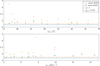 |
Fig. 18 Compilation for all simulations of the maximum HOG correlation coefficient, η, as a function of fCNM (top) and uRMS (bottom). The data points show η measured in orientations of the LOS parallel (green) and perpendicular (yellow) to the mean magnetic field. The dashed line at η = 1 separates the CNM-dominated (η < 1) from the WNM-dominated (η > 1) regime. The observed value in the 3C196 field is ηobs = 0.72. |
5.2 CNM-Faraday tomographic data correlation
Even though the numerical experiment presented here reveals a significant correlation between CNM and Faraday structures, when we looked closely we could not find a single example in our simulation set that would perfectly reproduce the relative correlation of CNM and WNM with the Faraday tomographic data (i.e., η).
The Faraday depth values observed in the 3C196 field are almost centered on zero (see M1 in Fig. 9, left). As mentioned in Jelić et al. (2018), this implies that the magnetic field is likely close to perpendicular to the LOS in this area of the sky. Indeed, we reproduced this feature (⟨M1⟩ ∼ 0) via synthetic observation with B perpendicular to the LOS, but the distribution of M1 and the range of Faraday spread (M2 ∼ 1–2.5 rad m−2) for this configuration are narrower than what is observed, even after de-biasing for noise.
Another important limitation concerns the physical size of the simulation box. The comparison between the simulated and observed Faraday depth distributions implicitly assumes that all polarized emission and rotation detected by LOFAR originate within a volume comparable to that of the simulation (50 pc on one side). In reality, the observed emission in the 3C196 field likely arises from a more extended region along the LOS, possibly spanning several hundred parsecs through the local magneto-ionic medium. This difference in physical depth may partly account for the narrower range of simulated Faraday depths and could also influence other derived quantities such as rotation-measure dispersion and the H i–polarization correlations. Nevertheless, achieving realistic CNM structures requires sub-parsec resolution, which cannot be maintained in simulations spanning Galactic-scale path lengths.
Regarding the H i-Faraday correlation, the B ⊥ LOS case is the one for which the values of η depart the most from the observations. As shown in Figures 13 and 16, the CNM shows significantly smaller values of  than the WNM (i.e., higher values of η) than in the case where B is parallel to the LOS. The only way to obtain η values close to the ones of the 3C196 field is by adding unrealistically large noise in the 21 cm synthetic data – i.e., ten times the one present in the real EBHIS data – in order to significantly affect the 21 cm WNM signal, but not as much the CNM. The case with B ∥ LOS produces values of η that are closer to the observed ones, but this configuration shows values of M1 that are significantly larger than the observations. A larger CNM-F(ϕ) correlation (i.e., lower values of η) could be produced by an increase of ne in the dense H i, producing a stronger Faraday signature associated with CNM structures. This could be adjusted by modifying the post-processing prescription used to estimate ne locally. Another way would be a stronger morphological correlation between the CNM filamentary structures and the orientation of B. We noticed in our simulations that many CNM clouds seem to have a random orientation with respect to B (see Fig. 2). This might require another forcing scheme for the simulations, perhaps using stellar feedback (e.g. supernovae) that might introduce coherent high pressure fronts over larger scales.
Finally, another way to lower η would be to have a lower correlation between the WNM and the Faraday structure. This could be caused by the WIM itself, which we did not model in our setup. The WIM is likely to have a diffuse structure, similar to the WNM, with more large-scale fluctuations. If the WIM is not spatially correlated to the WNM, its contribution to the Faraday deptH is likely to affect the WNM-Faraday correlation more than the CNM one. The same is true if one considers the fact that the LOS in the 3C196 field is likely to be about four times larger than what is modeled here. Adding up WNM signal along the LOS could lower the morphological correlation between the WNM and Faraday. As the CNM occupies smaller volumes along the LOS, it is less affected by the projection effect of long LOSs. All these effects are beyond the scope of this work, but they could be tested with dedicated numerical setups. Finally, our comparison relied entirely on a single LOFAR field, and thus it sampled a limited volume of the local ISM. The magnetic and thermodynamic conditions along this LOS may not be representative of other regions of the sky. Consequently, any correspondence between simulations and observations should be interpreted as illustrative rather than universally representative of the Galactic ISM that could be tested with the whole LoTSS mosaic (e.g., Erceg et al. 2022; Erceg et al. 2024).
5.3 Depolarization canals
A second aspect that is not well reproduced by our numerical setup is that of depolarization canals. We observe them in our simulations, and some seem to be caused by beam depolarization. On the other hand, the morphology of the synthetic depolarization canals do not match the observations. Depolarization canals observed in the 3C196 field and over large areas at high Galactic latitude (Erceg et al. 2022) are often very elongated, with axis ratios from ten to 100. The depolarization canals produced in our instrumental experiment are more twisty and relatively short.
This calls for another numerical study with the properties of the magnetic field (we used a single value for the initial B) and those of the mechanism injecting kinetic energy in the system varied more. One might want to explore supernova feedback or, alternatively, Fourier driving with different timescales and/or with a more consistent orientation. In general, turbulence-in-a-box simulations have a hard time producing very elongated CNM features, even in cases where they are found to be aligned with B (Inoue & Inutsuka 2016).
6 Conclusion
The main goal of this study was to evaluate if current state-of-the-art MHD numerical experiments used to model the thermally bistable H i are able to reproduce properties of the Faraday sky and, in particular, the H i-Faraday correlation observed in the LOFAR data (e.g., Bracco et al. 2020). Our parametric study is based on 50 pc simulation boxes (MHD + cooling) with a range of turbulent-velocity forcing with different amplitudes and levels of compressibility. The forcing led to realistic ranges of velocity dispersion, CNM fraction, and magnetic-field fluctuations, reproducing values observed in the diffuse ISM. From this set, we produced synthetic 21 cm and synchrotron observations, including the effect of noise and the LoTSS uv minimum, exploring a range of orientations of the LOS from parallel to perpendicular to the mean B field.
Our study reveals that thermal electrons associated with the H i phase could contribute a significant fraction of the low-frequency (100–200 MHz) synchrotron polarized emission observed at high Galactic latitudes. Indeed, our synthetic Fara-day observations reproduce levels of polarization intensity and RM values that are commensurate with what was observed with LOFAR in the 3C196 field, our test region.
To study the contribution of CNM structures to the Faraday tomographic structures in more detail, we developed a metric, η, based on the HOG algorithm (Soler et al. 2019) that measures the ratio of WNM to CNM spatial correlation between 21 cm velocity channels and polarized intensity at specific Faraday depths. We show that this metric is quite robust with respect to the kernel size of the HOG algorithm. Our analysis reveals a significant correlation of the CNM with Faraday structures, similar to what is observed in the 3C196 field (Bracco et al. 2020). The level of CNM-F(ϕ) correlation specifically depends on several factors, which we list below:
Simulations with low turbulent motions tend to have a stronger H i-Faraday correlation in general, and also smaller η;
The CNM-F(ϕ) correlation level depends on the B − LOS orientation; B perpendicular (parallel) to the LOS shows the lowest (highest) CNM-F(ϕ) correlation;
A larger CNM-F(ϕ) correlation can be measured in faint and noisy 21 cm data as higher 21 cm noise tends to affect the broad and low-brightness WNM more compared to the sharper and brighter CNM components;
Noise in Faraday data reduces the level of correlation of all H i phases equivalently, while not affecting η;
Finally, the level of CNM-F(ϕ) correlation does not depend strongly on fCNM. We observe a very mild increase in CNM-F(ϕ) correlation with fCNM, and only for fCNM < 20% and in the case where the LOS is perpendicular to the mean B field.
Within the space we explored, the CNM is always correlated with the Faraday tomographic structures, but we were not able to precisely reproduce values of η as low as those found in the 3C196 field (η = 0.72). This indicates that CNM structures are more correlated to Faraday structures in the observations than what we were able to reproduce with our numerical experiment. This is specifically true if we consider simulations with physical conditions similar to the 3C196 field (B ⊥ LOS, σu,1pc = 2.0 km s−1, and fCNM = 38%). In these conditions, we find η ∼ 1.5, whicH indicates that WNM contributes more to Faraday structures than the CNM. Several elements could contribute to this result: the choice of the ne prescription, the contribution of the WIM to the Faraday depths (not modeled), the longer length of the LOS in the data compared to the simulations, and the Fourier driving that tends to produce CNM structures not aligned with B.
Our results are indicative that low-frequency observations could serve as a probe of the magnetic-field intensity and morphology in the neutral edges of the Local Bubble. Moreover, the detailed comparison of simulations and observations in the 21 cm Faraday space revealed subtle discrepancies that call for an improvement of the way the multiphase, turbulent, magnetized, and partly ionized ISM is modeled today.
Finally, we note that our conclusions are drawn from the comparison with a single observational field. Future work should extend this analysis to additional LOFAR fields to test the robustness and generality of the trends identified here across different Galactic environments.
References
- Audit, E., & Hennebelle, P. 2005, A&A, 433, 1 [CrossRef] [EDP Sciences] [Google Scholar]
- Bellomi, E., Godard, B., Hennebelle, P., et al. 2020, A&A, 643, A36 [NASA ADS] [CrossRef] [EDP Sciences] [Google Scholar]
- Bezanson, J., Edelman, A., Karpinski, S., & Shah, V. B. 2017, SIAM Rev., 59, 65 [Google Scholar]
- Boulanger, F., Gry, C., Jenkins, E. B., et al. 2024, A&A, 687, A102 [NASA ADS] [CrossRef] [EDP Sciences] [Google Scholar]
- Bracco, A., Jelić, V., Marchal, A., et al. 2020, A&A, 644, L3 [EDP Sciences] [Google Scholar]
- Bracco, A., Ntormousi, E., Jelić, V., et al. 2022, A&A, 663, A37 [NASA ADS] [CrossRef] [EDP Sciences] [Google Scholar]
- Brentjens, M. A., & de Bruyn, A. G. 2005, A&A, 441, 1217 [NASA ADS] [CrossRef] [EDP Sciences] [Google Scholar]
- Burn, B. J. 1966, MNRAS, 133, 67 [Google Scholar]
- Cabral, B., & Leedom, L. C. 1993, in Proceedings of the 20th Annual Conference on Computer Graphics and Interactive Techniques, 263 [Google Scholar]
- Clark, S. E., & Hensley, B. S. 2019, ApJ, 887, 136 [NASA ADS] [CrossRef] [Google Scholar]
- Clark, S. E., Hill, J. C., Peek, J. E. G., Putman, M. E., & Babler, B. L. 2015, Phys. Rev. Lett., 115, 241302 [Google Scholar]
- Dickey, J. M., Landecker, T. L., Thomson, A. J. M., et al. 2019, ApJ, 871, 106 [NASA ADS] [CrossRef] [Google Scholar]
- Edenhofer, G., Zucker, C., Frank, P., et al. 2024, A&A, 685, A82 [NASA ADS] [CrossRef] [EDP Sciences] [Google Scholar]
- Erceg, A., Jelić, V., Haverkorn, M., et al. 2022, A&A, 663, A7 [NASA ADS] [CrossRef] [EDP Sciences] [Google Scholar]
- Erceg, A., Jelić, V., Haverkorn, M., et al. 2024, A&A, 688, A200 [NASA ADS] [CrossRef] [EDP Sciences] [Google Scholar]
- Eswaran, V., & Pope, S. B. 1988, Comput. Fluids, 16, 257 [NASA ADS] [CrossRef] [Google Scholar]
- Ferrière, K. M. 2001, Rev. Mod. Phys., 73, 1031 [NASA ADS] [CrossRef] [Google Scholar]
- Ferrière, K., West, J. L., & Jaffe, T. R. 2021, MNRAS, 507, 4968 [Google Scholar]
- Field, G. B. 1965, ApJ, 142, 531 [Google Scholar]
- Fromang, S., Hennebelle, P., & Teyssier, R. 2006, A&A, 457, 371 [NASA ADS] [CrossRef] [EDP Sciences] [Google Scholar]
- Ginzburg, V. L., & Syrovatskii, S. I. 1965, ARA&A, 3, 297 [Google Scholar]
- Godard, B., des Forêts, G. P., & Bialy, S. 2024, A&A, 688, A169 [NASA ADS] [CrossRef] [EDP Sciences] [Google Scholar]
- Haverkorn, M., & Heitsch, F. 2004, A&A, 421, 1011 [NASA ADS] [CrossRef] [EDP Sciences] [Google Scholar]
- Heiles, C., & Troland, T. H. 2003, ApJ, 586, 1067 [NASA ADS] [CrossRef] [Google Scholar]
- Heiles, C., & Troland, T. H. 2005, ApJ, 624, 773 [NASA ADS] [CrossRef] [Google Scholar]
- Hutschenreuter, S., Anderson, C. S., Betti, S., et al. 2022, A&A, 657, A43 [NASA ADS] [CrossRef] [EDP Sciences] [Google Scholar]
- Inoue, T., & Inutsuka, S.-I. 2016, ApJ, 833, 10 [Google Scholar]
- Jelić, V., de Bruyn, A. G., Pandey, V. N., et al. 2015, A&A, 583, A137 [Google Scholar]
- Jelić, V., Prelogović, D., Haverkorn, M., Remeijn, J., & Klindžić, D. 2018, A&A, 615, L3 [NASA ADS] [CrossRef] [EDP Sciences] [Google Scholar]
- Kerp, J., Winkel, B., Ben Bekhti, N., Flöer, L., & Kalberla, P. 2011, Astron. Nachr., 332, 637 [NASA ADS] [CrossRef] [Google Scholar]
- Kolmogorov, A. 1941, Akad. Nauk SSSR Dokl., 30, 301 [Google Scholar]
- Longair, M. S. 2011, High Energy Astrophysics (Cambridge University Press) [Google Scholar]
- Marchal, A., & Miville-Deschênes, M.-A. 2021, ApJ, 908, 186 [NASA ADS] [CrossRef] [Google Scholar]
- Marchal, A., Miville-Deschênes, M.-A., Orieux, F., et al. 2019, A&A, 626, A101 [NASA ADS] [CrossRef] [EDP Sciences] [Google Scholar]
- Marchal, A., Martin, P. G., Miville-Deschênes, M.-A., et al. 2024, ApJ, 961, 161 [NASA ADS] [CrossRef] [Google Scholar]
- Mininni, C., Molinari, S., Soler, J. D., et al. 2025, A&A, 699, A34 [NASA ADS] [CrossRef] [EDP Sciences] [Google Scholar]
- Orlando, E. 2018, MNRAS, 475, 2724 [NASA ADS] [CrossRef] [Google Scholar]
- Padovani, M., & Galli, D. 2018, A&A, 620, L4 [NASA ADS] [CrossRef] [EDP Sciences] [Google Scholar]
- Padovani, M., Bracco, A., Jelić, V., Galli, D., & Bellomi, E. 2021, A&A, 651, A116 [NASA ADS] [CrossRef] [EDP Sciences] [Google Scholar]
- Padovani, M., Bialy, S., Galli, D., et al. 2022, A&A, 658, A189 [NASA ADS] [CrossRef] [EDP Sciences] [Google Scholar]
- Planck Collaboration Int. XXXII. 2016, A&A, 586, A135 [NASA ADS] [CrossRef] [EDP Sciences] [Google Scholar]
- Rashidi, A., Yahia, H., Bontemps, S., et al. 2024, A&A, 688, A91 [NASA ADS] [CrossRef] [EDP Sciences] [Google Scholar]
- Rybicki, G. B., & Lightman, A. P. 1979, Astron. Q., 3, 199 [Google Scholar]
- Saury, E., Miville-Deschênes, M. A., Hennebelle, P., Audit, E., & Schmidt, W. 2014, A&A, 567, A16 [NASA ADS] [CrossRef] [EDP Sciences] [Google Scholar]
- Sokoloff, D. D., Bykov, A. A., Shukurov, A., et al. 1998, MNRAS, 299, 189 [Google Scholar]
- Soler, J. D., Beuther, H., Rugel, M., et al. 2019, A&A, 622, A166 [NASA ADS] [CrossRef] [EDP Sciences] [Google Scholar]
- Takahashi, K. 2023, PASJ, 75, S50 [Google Scholar]
- Teyssier, R. 2002, A&A, 385, 337 [CrossRef] [EDP Sciences] [Google Scholar]
- Turić, L., Jelić, V., Jaspers, R., et al. 2021, A&A, 654, A5 [NASA ADS] [CrossRef] [EDP Sciences] [Google Scholar]
- Van Eck, C. L. 2018, Galaxies, 6, 112 [NASA ADS] [CrossRef] [Google Scholar]
- Van Eck, C. L., Haverkorn, M., Alves, M. I. R., et al. 2017, A&A, 597, A98 [NASA ADS] [CrossRef] [EDP Sciences] [Google Scholar]
- van Haarlem, M. P., Wise, M. W., Gunst, A. W., et al. 2013, A&A, 556, A2 [NASA ADS] [CrossRef] [EDP Sciences] [Google Scholar]
- Winkel, B., Kerp, J., Flöer, L., et al. 2016, A&A, 585, A41 [NASA ADS] [CrossRef] [EDP Sciences] [Google Scholar]
- Wolfire, M. G., McKee, C. F., Hollenbach, D., & Tielens, A. G. G. M. 2003, ApJ, 587, 278 [Google Scholar]
Appendix A MOOSE
Mock Observation of Synchrotron Emission (
MOOSE) is an interactive Julia-based tool designed to process numerical simulations of synchrotron emission and Faraday rotation. It generates synthetic observations by integrating three-dimensional cubes of physical parameters, including density, temperature, and magnetic-field components. The electron density is computed using either empirical prescriptions or direct scaling with the neutral hydrogen density.
The code reconstructs polarization properties by computing synchrotron emission and applying Faraday rotation effects along the LOS. It accounts for observational constraints by filtering large-scale structures to matcH interferometric data, convolving signals with telescope beam responses, and incorporating noise models to replicate real observations.
MOOSEemploys 2D interpolation methods to efficiently estimate synchrotron emissivities based on precomputed lookup tables. The interpolation grid is currently designed to use LOFAR frequencies but can be adapted to any frequency range depending on the observational requirements. This technique allows for accurate integration of synchrotron radiation over a range of magnetic field strengths and frequencies while maintaining computational efficiency.
The code first reconstructs the Stokes parameters (Iν, Qν, Uν) as a function of frequency before applying
RM-Synthesisto derive the Faraday spectrum. This approach enables the decomposition of polarized emission along different Faraday depths, making it possible to analyze the magneto-ionic properties of the ISM.
The tool assumes an optically thin medium, meaning absorption effects are neglected. While this assumption is generally valid for high Galactic latitude regions, it may introduce biases in denser environments.
The synthetic data can be analyzed to extract rotation measure maps, Faraday spectra, and polarization structures.
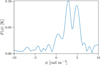 |
Fig. A.1 Example of a Faraday spectrum produced by MOOSE. The x-axis represents the Faraday deptH in rad m−2, while the y-axis corresponds to the polarized intensity. The two primary peaks are located at ϕ1 = 2.75 rad m−2 and ϕ2 = 5 rad m−2. |
Figure A.1 represents an example of the polarized intensity as a function of the Faraday depth (in rad m2). Peaks in the spectrum indicate distinct polarized emission components along the LOS. The two most significant peaks in the spectrum correspond to Faraday depths of approximately ϕ1 = 2.75 rad m−2 and ϕ2 = 5 rad m−2, which likely indicate separate emitting regions along the LOS.
It provides a visual representation of how
MOOSEreconstructs the Faraday spectrum from input simulation data. The presence of sidelobes in the spectrum is a common feature resulting from the limited frequency coverage and resolution in
RM-Synthesis. These sidelobes can introduce ambiguities in identifying true polarized components.
Appendix B Faraday moments
M0 is the polarized intensity integrated over the Faraday depth range. M1 is the polarized intensity weighted mean of Faraday depth ϕ. M2 is the width of the Faraday spectrum. These are analogous to moments in velocity space and are fully described in Dickey et al. (2019). These quantities are affected by noise; moments are often estimated by thresholding the data, for instance Erceg et al. (2022) used only values six times higher than the noise level. Here we propose alternatives to estimate the Faraday moments without rejecting any data.
Because F(ϕ) is a strictly positive quantity, noise in F(ϕ) has a specific effect. Noise fluctuations do not cancel out in calculating M0 but they add up introducing a bias. For a given noise level σnoise (computed here by taking the standard deviation at the first 30 and the last 30 Faraday depths ϕ) the noise bias on the first moment is equal to N σnoise where N is the number of Faraday depths. To take this into account we compute the first moment as
 (B.1)
(B.1)
where dϕ is the channel widtH in ϕ.
The second-order moment M2 is also affected by noise but it is also very sensitive to the presence of sidelobes in Faraday spectra (see an example in Fig. A.1). These sidelobes arise from the limited range of λ2 over which the Fourier transform is computed (see Eq. (12)). The spectral shape of F(ϕ) also depends significantly on the spectral shape of Qν and Uν that can vary significantly due to Faraday rotation (Equations (7) and (8)). This results in spectral structures in P(λ2) that can vary significantly from one position to the next. These spectral features in P(λ2) are not instrumental as they depend on the physical distribution of emitting and rotating structures along the LOS (Takahashi 2023). In certain conditions the combination of Qν and Uν can even cancels signal in P(λ2). As a consequence, the width of the Faraday spectrum can, in some cases, be smaller than the width of the RMSF, making its interpretation difficult.
As an alternative, we estimated the width of the Faraday spectrum using the effective width defined as
 (B.2)
(B.2)
This quantity reduces the influence of sidelobes by emphasizing the integrated power of the spectrum relative to its peak intensity. We found that Weff provides a more robust and interpretable characterization of the spectral widtH in the presence of complex interference patterns. It is also not biased by noise like a standard second moment is. We computed Weff using M0 corrected for the noise bias. Then the second order moment is estimated as
 (B.3)
(B.3)
whicH is the exact solution for a Gaussian function.
Finally, the first moment M1 defined as
 (B.4)
(B.4)
is also biased in the presence of noise. As noise increases, the numerator tends to produce M1 → ⟨ϕi⟩. If the ϕ vector is centered on 0, like it is the case in our study, lower S/N F(ϕ) will tend to have M1 → 0. To circumvent this effect, we are using a matched filter approach. We leverage on the fact that Weff is a non biased estimate of the width of the signal, especially if the complexity of the Faraday spectra is small (i.e., F(ϕ) is characterized by one dominating component, large or narrow). The first moment is found by convolving F(ϕ) by a Gaussian filter with a width given by Weff. M1 is then estimated at the value of ϕ where this convolution is maximum.
Appendix C HOG results for the whole set of simulations
The results of the HOG analysis for the whole 14 simulations set are presented in Fig. C.1 (B parallel to the LOS) and Fig. C.2 (B perpendicular to the LOS). Different color backgrounds are used to illustrate low (vRMS < 8 km s−1 – gray background) and high (vRMS > 8 km s−1 – light blue background) turbulence level.
Appendix D Rotation of the cubes
To analyze physical quantities along different lines of sight, it is necessary to rotate the simulation cubes containing both scalar and vector fields. The rotation is particularly important in the context of these simulations because the magnetic field has a preferred orientation with a strong mean component in a specific direction. In our simulations, the ratio of the mean field strength to the root-mean-square fluctuation (B/Brms) is large, meaning that the field is strongly ordered. As a result, analyzing the simulations only along the three cartesian orientations provides a limited perspective on the system.
By rotating the cubes by arbitrary angles, it becomes possible to explore configurations that are not perfectly aligned with the dominant field direction. This is crucial for understanding how turbulence and ordered structures interact under different projection effects. It also allows for a more comprehensive analysis of how observables change with different viewing angles.
Rotation of scalar fields
For scalar fields such as electron density (ne), temperature (T), and neutral hydrogen density (nH), the rotation consists of a coordinate transformation from the original frame (x, y, z) to the new frame (x′, y′, z′). Given a rotation matrix R, the new coordinates are obtained as:
![Mathematical equation: $\left[ {\matrix{{x'} \hfill \cr {y'} \hfill \cr {z'} \hfill \cr } } \right] = R\left[ {\matrix{x \hfill \cr y \hfill \cr z \hfill \cr } } \right].$](/articles/aa/full_html/2026/04/aa57351-25/aa57351-25-eq74.png) (D.1)
(D.1)
The scalar field values remain unchanged at each transformed coordinate. In practice, the rotation is implemented by interpolating the values of the scalar field onto the rotated grid using bilinear interpolation.
Rotation of vector fields
For vector fields such as the magnetic field components (Bx, By, Bz) and velocity components (Vx, Vy, Vz), both the coordinate system and the vector components must be rotated. If the original vector field is represented as:
![Mathematical equation: $U = \left[ {\matrix{{{U_x}} \hfill \cr {{U_y}} \hfill \cr {{U_z}} \hfill \cr } } \right],$](/articles/aa/full_html/2026/04/aa57351-25/aa57351-25-eq75.png) (D.2)
(D.2)
then after rotation, the new components are given by:
 (D.3)
(D.3)
where R is the same 3 × 3 orthogonal rotation matrix applied to the coordinate system. However, to correctly rotate a vector field, it is necessary to first apply the inverse transformation to determine where in the original coordinate system the vector should be sampled, and then apply the rotation to the vector itself:
 (D.4)
(D.4)
These transformations ensure that the rotated vector components remain physically meaningful and aligned with the new coordinate system.
Figure D.1 shows maps of Pmax and column density of the case-study simulation rotated around the z-axis by a 45◦. Fig. D.2 shows the result of HOG in this configuration.
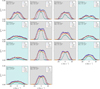 |
Fig. C.1 HOG results for all the set of simulations for the orientation of the LOS parallel to mean B. In each panel the curve |

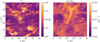 |
Fig. D.1 Maximum polarized intensity (left) and column density (right) of the case-study simulation rotated by 45◦ around the z-axis. |
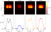 |
Fig. D.2 HOG results for the 45◦ configuration shown in Fig. D.1. The values of |

All Tables
All Figures
|
Fig. 1 Moment 0 (integrated polarized intensity) de-biased for noise (top), Moment 1 (middle) and Moment 2 (bottom) of the 3C196 field from LOFAR LoTSS DR2 Faraday tomographic data (Erceg et al. 2022). |
| In the text | |
|
Fig. 2 Slice through the simulation cube showing the logarithmic gas density overlaid with magnetic-field orientation using the line integral convolution (LIC) technique. Left: projection along the mean magnetic-field direction. Right: projection perpendicular to the mean field. |
| In the text | |
|
Fig. 3 CNM mass fraction, fCNM, of the different simulations used in this study. The dashed circles highlight the simulations with the same turbulent mode ratio, χ. Colors show the initial input for the forcing amplitude. |
| In the text | |
|
Fig. 4 M1 distributions as a function of fCNM for the set of simulations. These distributions are measured along two orthogonal directions: parallel (lighter color) and perpendicular (darker color) to the mean magnetic field. Filled circles indicate the corresponding mean values ⟨M1⟩, outlined in black. The case-study simulation is highlighted in red, while the remaining simulations are shown in violet. Two simulations have fCNM = 26%, leading to an overplotting of their respective distributions. The 3C196 field is displayed in blue witH its associated distribution and mean value. |
| In the text | |
|
Fig. 5 Simulation 7. RM histograms for cubes produced with the LOS parallel, perpendicular, or 45◦ to the mean direction of B. Dashed lines: mean values of the rotation measure maps. The mean values are ⟨RM∥⟩ = 5.5 rad m−2, ⟨RM⊥⟩ = 0.0 rad m−2, and ⟨RM45◦ ⟩ = 3.9 rad m−2. |
| In the text | |
|
Fig. 6 Mock observations for simulation 7 in the case where the LOS is parallel to the mean B field. Left panel: map of Faraday spectrum F(ϕ) at ϕ = 1.75 rad m−2. Right panel: map of 21 cm brightness temperature TB(u) for v = 0.9 km s−1. |
| In the text | |
|
Fig. 7 Column density (left panels) and Faraday moment maps (right panels) for case-study simulation, witH integration along the mean magnetic field. Top to bottom: logarithmic column-density maps of total H i, CNM, and WNM; moments 0, 1, and 2 of the Faraday spectrum. |
| In the text | |
|
Fig. 8 Same as Fig. 7, but for the case where the LOS is perpendicular to the mean magnetic field. Due to the weak LOS magnetic component, M1 values remain close to zero and M2 is narrower across the field. While the density structures of CNM and WNM are similar to the parallel case, the Faraday moments show significantly reduced signal, consistent with expectations for a transverse magnetic-field configuration. |
| In the text | |
|
Fig. 9 Probability density functions of Faraday spectral moments for the 3C196 field (gray) and for the case-study simulation with three magnetic field orientations: parallel (yellow), perpendicular (blue), and rotated 45◦ (green). Left: first-order moment, M1, showing higher values in the parallel case and near-zero mean in the perpendicular case. Right: second-order moment, M2, of the Faraday spectrum. |
| In the text | |
|
Fig. 10 Maximum polarized-intensity maps (Pmax) from the case-study simulation, illustrating the presence and morphology of depolarization canals. Left: integration along the LOS parallel to the mean magnetic field. Right: integration perpendicular to the mean field. Linear, canal-like features are prominent in the parallel case, while more circular structures dominate in the perpendicular configuration. |
| In the text | |
|
Fig. 11 HOG |
| In the text | |
|
Fig. 12 HOG |
| In the text | |
|
Fig. 13 HOG |
| In the text | |
|
Fig. 14 Effect of increasing noise in H i data on the HOG correlation with Faraday tomography structures for the case-study simulation along the mean field. Each panel displays the 98th percentile of the normalized Rayleigh statistic |
| In the text | |
|
Fig. 15 Impact of increasing noise in the Faraday data on the HOG correlation between phase-separated H i structures and Faraday depth features for the case-study simulation along the mean field Each panel shows the 98th percentile of the normalized Rayleigh statistic ( |
| In the text | |
|
Fig. 16 Dependence of HOG correlation maxima ratio, η, on the derivative kernel size used in the gradient computation for different levels of Gaussian noise added to the H i data. Left: case-study simulation with the magnetic field aligned with the LOS. Right: same simulation, but with the mean field perpendicular to the LOS. The observational value from the 3C196 field is shown for comparison (dashed line). |
| In the text | |
|
Fig. 17 Compilation for all simulations of the maximum value of the 98th percentile of the normalized Rayleigh statistic |
| In the text | |
|
Fig. 18 Compilation for all simulations of the maximum HOG correlation coefficient, η, as a function of fCNM (top) and uRMS (bottom). The data points show η measured in orientations of the LOS parallel (green) and perpendicular (yellow) to the mean magnetic field. The dashed line at η = 1 separates the CNM-dominated (η < 1) from the WNM-dominated (η > 1) regime. The observed value in the 3C196 field is ηobs = 0.72. |
| In the text | |
|
Fig. A.1 Example of a Faraday spectrum produced by MOOSE. The x-axis represents the Faraday deptH in rad m−2, while the y-axis corresponds to the polarized intensity. The two primary peaks are located at ϕ1 = 2.75 rad m−2 and ϕ2 = 5 rad m−2. |
| In the text | |
|
Fig. C.1 HOG results for all the set of simulations for the orientation of the LOS parallel to mean B. In each panel the curve |
| In the text | |
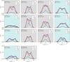 |
Fig. C.2 Same as Fig. C.1 but for cases where the LOS is perpendicular to mean B. |
| In the text | |
|
Fig. D.1 Maximum polarized intensity (left) and column density (right) of the case-study simulation rotated by 45◦ around the z-axis. |
| In the text | |
|
Fig. D.2 HOG results for the 45◦ configuration shown in Fig. D.1. The values of |
| In the text | |
Current usage metrics show cumulative count of Article Views (full-text article views including HTML views, PDF and ePub downloads, according to the available data) and Abstracts Views on Vision4Press platform.
Data correspond to usage on the plateform after 2015. The current usage metrics is available 48-96 hours after online publication and is updated daily on week days.
Initial download of the metrics may take a while.