| Issue |
A&A
Volume 708, April 2026
|
|
|---|---|---|
| Article Number | A204 | |
| Number of page(s) | 20 | |
| Section | Catalogs and data | |
| DOI | https://doi.org/10.1051/0004-6361/202558132 | |
| Published online | 08 April 2026 | |
The S-PLUS Fornax Project (S+FP): An extragalactic catalog covering ∼5 virial radii around NGC1399 with galaxy properties
1
Instituto de Astrofísica de La Plata, UNLP-CONICET,
Paseo del Bosque s/n,
La Plata,
B1900FWA,
Argentina
2
Facultad de Ciencias Astronómicas y Geofísicas, Universidad Nacional de La Plata,
Paseo del Bosque s/n,
La Plata,
B1900FWA,
Argentina
3
Departamento de Astronomia, Instituto de Astronomia, Geofísica e Ciências Atmosféricas da USP, Cidade Universitária,
05508-090
São Paulo,
SP,
Brazil
4
Institute of Astrophysics, Facultad de Ciencias Exactas, Universidad Andrés Bello,
Sede Concepción, Talcahuano,
Chile
5
Departamento de Tecnologías Industriales, Facultad de Ingeniería, Universidad de Talca,
Los Niches km 1,
Curicó,
Chile
6
International Gemini Observatory/NSF’s National Optical-Infrared Research Laboratory,
Casilla 603,
La Serena,
Chile
7
Universidade do Vale do Paraíba,
Av. Shishima Hifumi, 2911,
São José dos Campos
SP 12244-000,
Brazil
8
Valongo Observatory, Federal University of Rio de Janeiro,
Ladeira Pedro Antonio 43,
Saude Rio de Janeiro
RJ 20080-090,
Brazil
9
Departamento de Astronomía, Universidad de La Serena,
Av. J. Cisternas 1200 N,
1720236
La Serena,
Chile
10
Observatório Nacional, Rua General José Cristino,
77, São Cristóvão,
20921-400
Rio de Janeiro RJ,
Brazil
11
Departamento de Física, Universidad Técnica Federico Santa María,
Avenida España
1680,
Valparaíso,
Chile
12
Millennium Nucleus for Galaxies (MINGAL),
Santiago,
Chile
13
Laboratório Nacional de Astrofísica,
Rua Estados Unidos 154,
Itajubá
37504-364
MG,
Brazil
14
GMTO Corporation
465 N. Halstead Street,
Suite 250
Pasadena,
CA
91107,
USA
15
Rubin Observatory Project Office,
950 N. Cherry Ave.,
Tucson,
AZ
85719,
USA
16
Departamento de Física – CFM – Universidade Federal de Santa Catarina,
PO BOx 476,
88040-900
Florianópolis,
SC,
Brazil
★ Corresponding author: This email address is being protected from spambots. You need JavaScript enabled to view it.
Received:
15
November
2025
Accepted:
28
January
2026
Abstract
Context. Observational extragalactic catalogs over wide sky areas are essential for uncovering the large-scale structure of the Universe. They allow, among other things, cosmological studies and density analyses that impose strong constraints on models of galaxy formation and evolution.
Aims. By taking advantage of the wide field images and the 12 optical bands of the Southern Photometric Local Universe Survey (S-PLUS), we aim to provide a catalog of galaxies located, in projection, toward the Fornax galaxy cluster, within ∼ 5 virial radii in right ascension (RA) and ∼3 virial radii in declination (Dec) around NGC 1399, the dominant galaxy of the cluster. Such a catalog will allow unprecedented large-scale structure studies in that sky region.
Methods. We developed supervised deep-learning algorithms, utilizing neural networks complemented by dimensionality-reduction techniques, to classify and separate spurious objects, stars and galaxies in a photometric catalog previously built for the S-PLUS Fornax Project (S+FP). That catalog was built using a combination of SExtractor configurations optimized for galaxy detection and characterization.
Results. A catalog of 119 580 galaxies was obtained in the direction of the Fornax cluster containing photometric information in the 12 optical bands of S-PLUS complemented with GALEX (UV), VHS-VISTA (NIR), and AllWISE (MIR) data. We estimate photometric redshifts (σNMAD ∼ 0.0219) with a lower limit of zlim ∼ 0.03. Stellar masses, star formation rates (SFRs), and D4000N index estimates were obtained through a machine-learning approach, by matching S-PLUS photometric data to SDSS spectroscopic data. The completeness of the catalog (72%) was calculated by comparing it with mock catalogs.
Conclusions. Taking into account our zlim, we were able to identify 119 230 background galaxies and to find 350 candidates to be Fornax members or infalling galaxies, which were not included in our compilation of 1005 galaxies previously reported in the literature. We were also able to classify the galaxies in our catalog as quiescent (43%), star forming (39%), and transition (18%) galaxies. In addition, 181 emission line galaxy (ELG) candidates were identified using the filter J0660. The spatial distribution of the galaxies in our catalog shows projected overdensities that match 158 background clusters identified by eROSITA. This confirms the robustness of our catalog in tracing real structures. In that context, we expect the extragalactic catalog of the S+FP to allow us to better understand the large-scale structure in the direction of the Fornax cluster and to identify the substructures that are feeding Fornax.
Key words: techniques: photometric / surveys / galaxies: clusters: general / galaxies: evolution / galaxies: individual: NGC 1399
© The Authors 2026
 Open Access article, published by EDP Sciences, under the terms of the Creative Commons Attribution License (https://creativecommons.org/licenses/by/4.0), which permits unrestricted use, distribution, and reproduction in any medium, provided the original work is properly cited.
This article is published in open access under the Subscribe to Open model. This email address is being protected from spambots. You need JavaScript enabled to view it. to support open access publication.
1 Introduction
Large, photometric extragalactic catalogs constitute a basic and straightforward tool for revealing the projected spatial distribution of the galaxy distribution in the sky and, as a consequence, for disclosing the large-scale structure of the Universe. Combined with additional information such as that provided by a density analysis and spectroscopic data (among other factors), they have allowed a number of studies in the cosmological field to explore the processes of galaxy group and cluster formation and to deepen our comprehension of the formation and evolution paths of the galaxies belonging to different environments.
In recent years, several photometric surveys have allowed the creation of large extragalactic catalogs. The Sloan Digital Sky Survey (SDSS; York et al. 2000) revolutionized observational astronomy with its imaging coverage of ∼14 000 deg2 of the northern sky in five optical broad bands (u, g, r, i and z). The Dark Energy Camera Legacy Survey (DECaLS; Dey et al. 2019) is more deeply mapping the southern hemisphere, through wide-field images in four optical bands (g, r, i and z). The Wide-field Infrared Survey Explorer (WISE; Wright et al. 2010) and the Vista Hemisphere Survey (VHS; McMahon et al. 2013) complement that optical data in the IR regime. For objects simultaneously included in those catalogs, the combination of photometry at different wavelengths opens the possibility of obtaining additional valuable information, such as photometric redshifts (zphot) and stellar masses, from the fit of their spectral energy distribution (SED). However, the combination of broad bands alone (such as those in the SDSS) brings limitations in estimating those parameters. To improve this issue, projects such as the Southern Photometric Local Universe Survey (S-PLUS; Mendes de Oliveira et al. 2019) and its northern counterpart, the Javalambre Photometric Local Universe Survey (J-PLUS; Cenarro et al. 2019), have implemented the Javalambre photometric system consisting of 12 optical broad and narrow bands. J-PAS (Benítez et al. 2015) went further by using 56 narrow bands in the optical range, which allowed for quasispectroscopic sampling of the continuum and emission lines of galaxies.
A fundamental aspect of the construction of a large extragalactic catalog, from automatic photometry performed in wide-field images using software such as SExtractor (Bertin & Arnouts 1996), is the separation of galaxies from compact sources and spurious confident detections. Several works have addressed this problem using morphological and photometric criteria, as well as through the application of machine-learning (ML) techniques. As an example of the latter approach, Bailer-Jones et al. (2019) used neural networks (NNs) and probabilistic models to perform a galaxy-quasar separation in Gaia Data Release 2.
Once a reliable multiband catalog of galaxies is obtained, the estimation of zphot becomes key to tracing large-scale structures. In general, those zphot can be obtained in two ways: via SED fitting or applying ML techniques. SEDfitting methods infer the redshift of a galaxy by comparing its observed photometry with stellar population models. These models can be observational, synthetic, or a combination of both. There are numerous codes that implement this approach, including LePhare (Arnouts et al. 1999; Ilbert et al. 2006), EAZY (Brammer et al. 2008), BAGPIPES (Carnall et al. 2018), CIGALE (Noll et al. 2011) and AlStar (Thainá-Batista et al. 2023), which is an adaptation of the spectral fitting code STARLIGHT (Cid Fernandes et al. 2005). Several studies have compared the accuracy of some of these codes under different observational conditions (see, e.g., Dahlen et al. 2013; Schmidt et al. 2020; Humire et al. 2025).
Photometric redshifts can also be estimated using ML algorithms, which have experienced a rapid development over the last decade due to their ability to model complex, nonlinear relationships in high-dimensional data. These methods include random forests, support vector machines, Gaussian processes, and deep NNs (Cavuoti et al. 2017; Pasquet et al. 2019; Zhou et al. 2021; Lima et al. 2022; Teixeira et al. 2024). Unlike SED fitting, which relies on physical models, ML approaches are purely empirical and require a representative training set with known spectroscopic redshifts. Once trained, these models can predict zphot with high computational efficiency, making them attractive for large datasets.
An important distinction between the two approaches lies in their performance across different redshift regimes. ML methods tend to display good performance at low redshifts (z ≲ 1), particularly when the training set is sufficiently dense and covers the relevant color space. However, their performance degrades at higher redshifts or in regions of parameter space not well represented in the training sample. In contrast, SED fitting methods, though typically slower and more sensitive to photometric uncertainties and template mismatches, are more robust when it comes to exploring regions of parameter space in which models can be physically extrapolated and can reach higher redshifts (Beck et al. 2017; Duncan et al. 2018).
Each approach has its own set of advantages and limitations. SED fitting provides not only redshift estimates, but also physical properties such as stellar masses, SFRs, and extinction values derived from the same model. However, it strongly depends on the choice of templates, priors, and assumptions about stellar population synthesis, which can introduce systematics. ML methods, by contrast, are more flexible and often achieve a lower scatter and lower outlier rates in well-calibrated regimes, but they may lack interpretability and are generally less suited to extrapolation. As a result, hybrid approaches that combine the strengths of both methods have also been proposed (D’Isanto & Polsterer 2018; Schmidt et al. 2020).
Besides redshift estimation, one of the most crucial parameters that an extragalactic catalog may provide is the galaxy stellar mass. Stellar mass is a fundamental quantity for understanding galaxy evolution, as it correlates with various physical properties such as star formation rate (SFR), metallicity, and morphology (Gallazzi et al. 2005; Peng et al. 2010). However, even when spectroscopic redshifts are available, the estimation of stellar masses is not straightforward. It typically involves fitting the galaxy’s SED with stellar population-synthesis models, which require assumptions about the initial mass function (IMF), dust attenuation, and star formation history. Variations in these assumptions can lead to systematic uncertainties of up to 0.3 dex in mass values (Conroy 2013; Pacifici et al. 2023). In photometric surveys, where redshift uncertainties propagate into the mass estimates, the challenges are even greater. Accurate redshifts are essential for robust mass determinations, especially for faint or high-redshift galaxies.
In addition, the identification of emission line galaxies (ELGs), such as [OII], Hα, and Lyman- α emitters, is of particular interest. These sources are often associated with active star formation or nuclear activity, and can serve as tracers of the cosmic web and large-scale structures (Cochrane et al. 2018; Khostovan et al. 2020). Their strong emission lines make them easy to detect and characterize, even in low signal-to-noise data, and their spatial distribution over large scales can reveal the underlying matter density field. Therefore, the combination of accurate zphot, stellar mass estimates, and emission line diagnostics is key to build comprehensive extragalactic catalogs that enable statistical studies of galaxy evolution and cosmology.
The Fornax cluster, located at a distance of ∼20 Mpc (z∼0.0046; Blakeslee et al. 2009), is the closest rich galaxy cluster after the Virgo cluster. Fornax is particularly interesting for studies of galaxy formation and evolution because of its dynamic structure, with a central concentration dominated by NGC 1399 and a significant population of dwarf galaxies. It also has a secondary substructure centered on NGC 1316 (Fornax A), which is falling toward the main structure (Scharf et al. 2005; Venhola et al. 2019). Furthermore, the Fornax cluster is part of the Eridanus–Fornax–Doradus complex. This large-scale structure was first identified in the context of the Southern Sky Redshift Survey by da Costa et al. (1998). According to these authors, the two most prominent structures in the 0 < v < 3000 kms−1 window, the Fornax cluster and the Eridanus group (Raj et al. 2024), appear to form a linear structure connected to the looser Dorado group (Kilborn et al. 2005).
The present work was developed in the context of the S-PLUS Fornax Project (S+FP; Smith Castelli et al. 2024), an initiative aimed at studying the Fornax galaxy cluster and its surroundings in 12 optical bands up to five virial radii (Rvir) in right ascension (RA) and ∼3 Rvir in declination (Dec). In this paper, we present an extragalactic catalog that allows us to analyze the large-scale distribution of galaxies in a projected sky area of ∼208 deg2 around NGC 1399. To that aim, we estimated zphot, stellar masses, the SFR, and the D4000N index, and we identified galaxies displaying an excess in the J0660 filter of S-PLUS that can be considered as ELG candidates.
This paper is structured as follows. Section 2 describes the photometric and spectroscopic data used. Section 3 details the methods of object classification and cleaning, including the categorization of stars, galaxies, and spurious objects. Section 4 presents the estimation of zphot, stellar masses, SFRs, and D4000N index values; an assessment of the accuracy of the methods used; and a lower limit in the estimation of zphot. Finally, Section 5 summarizes our results, presents the conclusions, and provides a discussion of possible future applications of this catalog.
2 Data
2.1 S-PLUS
The Southern Photometric Local Universe Survey (S-PLUS; Mendes de Oliveira et al. 2019) aims to map over 9000 deg2 of the southern sky using an 80-cm robotic telescope located at Cerro Tololo, Chile, equipped with a 12-band filter system. The uniqueness of S-PLUS is due to the use of seven narrowband filters (J0378, J0395 J0410, J0430, J0515, J0660, and J0861; Cenarro et al. 2019), developed specifically to probe interesting emission and absorption lines or bands in the nearby Universe such as [OII] 3727,3729, Ca H+K, Hδ, the G band, the Mgb triplet, Hα, and the Ca triplet.
In this work, we used the photometry presented by Haack et al. (2024), which was optimized to properly detect and characterize extragalactic objects. Our base catalog consists of a combination of the three catalogs, RUN1, RUN2, and RUN3, obtained in that work, avoiding the duplication of objects. It includes ∼3 × 10⁶ detected sources in a sky-projected area of ∼208 deg2 around NGC 1399, the dominant galaxy of the Fornax cluster. Those sources comprise galaxies, stars, and spurious objects. RUN 1 detected and performed the photometry for faint and small galaxies, especially those near bright galaxies; RUN 2 characterized galaxies that are intermediate in both brightness and size; and RUN 3 detected the largest galaxies, without subdividing them into several sources.
In the context of the S+FP, we established a reference sample of 1005 Fornax galaxies reported in the literature as spectroscopically confirmed members or probable members according to morphological criteria (for details on the compilation, we refer the reader to Smith Castelli et al. 2024). Hereafter, we refer to this sample as the Fornax literature sample (FLS).
2.2 Complementary photometric and spectroscopic data
To define the training sample for performing a star and galaxy separation, we use the probability for a source to be a star, a galaxy or a quasar from Gaia DR3 (Gaia Collaboration 2023).
In order to estimate zphot, we complemented the photometry provided by S-PLUS with magnitudes in the UV from GALEX (Bianchi et al. 2017), NIR from VHS DR5 (McMahon et al. 2013), and MIR from AllWISE (Cutri et al. 2013). The GALEX survey probed the entire sky using two UV bands, the NUV and FUV, with effective wavelengths of 2315.7 and 1538.6 Å, respectively, and typical depths of 19.9 and 20.8 AB mag. VHS observed the southern hemisphere using four NIR bands, namely Y (0.88 μm), J (1.03 μm), H (1.25 μm), and Ks (2.20 μm), with coverages of 4825, 16 689, 2901, and 16 684 deg2, respectively, and 5σ depths of 21.1, 20.8, 20.5, and 20.0 mag. This project observed more than one billion sources. WISE (Wright et al. 2010) is a NASA Medium Class Explorer mission that conducted a digital imaging survey of the entire sky in the 3.4, 4.6, 12, and 22 μm MIR bandpasses (hereafter W1, W2, W3, and W4). The AllWISE program extends the work of the successful WISE mission by combining data from the cryogenic and post-cryogenic survey phases to provide the most comprehensive view of the MIR sky currently available. In Section 4.1, we describe how we used spectroscopic redshifts collected by Lima et al. (2022) and obtained from SIMBAD to validate our estimations of zphot. In Sections 4.2 and 4.3, we outline our use of data from SDSS DR8 (Aihara et al. 2011) and physical parameters from Kauffmann et al. (2003), Brinchmann et al. (2014), and Tremonti et al. (2004) to estimate, through a ML approach, zphot, stellar masses, SFRs, and D4000N index values for all the objects in the S+FP extragalactic catalog.
3 Methodology
3.1 Spurious-object identification
As a starting point, each of the RUN 1, RUN 2 and RUN 3 catalogs (Haack et al. 2024) was taken separately and cleaned by internal duplications, performing a cross-match in RA and Dec coordinates with a 3-arcsec error. This corresponds to approximately six pixels of separation in the S-PLUS images.
In order to separate spurious objects from galaxies and stars (non-spurious objects), we define spurious detections in two categories: those arising at the edges of the images and those detected on the extended spikes of saturated stars. The S-PLUS DR4 images have lines or columns with null signal values over several pixels at their edges. In those regions, the mesh used by SExtractor for sky estimation finds null and non-null values, which results in a false estimation of the sky level. On the other hand, spurious objects that accumulate very close to the spikes of saturated stars, especially the brightest ones, arise because the signal from the pattern of the spikes prevents an efficient background assessment by SExtractor. Both cases are illustrated in Figure 1.
Once the spurious objects were defined, a supervised classification algorithm was developed using NNs to separate nonspurious and spurious detections. The NN architecture used consists of three hidden layers (256, 128, and 64 neurons) with ReLU activation (Nair & Hinton 2010) and L2 regularization (0.001) to mitigate overfitting (Ng 2004). Dropout (0.3) was applied to improve generalization and prevent excessive co-adaptation of neurons (Srivastava et al. 2014). The output layer uses a softmax function with two units for binary classification, employing a sparse categorical cross-entropy as a loss function, and Adam as an optimizer (Kingma & Ba 2017).
The learning of the NN to perform the classification is based on the photospectra of each of the sources, which is a discrete sequence of multiband magnitudes or fluxes that approximate the SED of an astrophysical source. Specifically, the input of the algorithm consists of the 12 AUTO (Kron-like; Kron 1980) magnitudes and their respective errors. Examples of different photospectra corresponding to a quasar, a main-sequence star, an early-type galaxy, a planetary nebula, and a symbiotic star, can be seen in Figure 7 of Mendes de Oliveira et al. (2019).
To define the training and testing samples, we manually labeled both types of spurious objects and rigorously checked each of them. In addition, we labeled stars (CLASS_STAR_r > 0.95) and galaxies (CLASS_STAR_r < 0.35) with r band magnitudes below 21.3, taking into account that the labeled objects are of different sizes, brightnesses and colors, as well as of different morphologies in the case of galaxies. CLASS_STAR is the stellarity index given by SExtractor. Stars and galaxies constitute the non-spurious category. Our training and testing samples thus include 3427 spurious objects (half of them are detections at the edges of the images and the other half corresponds to identifications near stars spikes); 6854 are non-spurious objects (including stars and galaxies). Since the sample is not balanced between these two categories, the NN classification adopted stratified K-Fold cross-validation (Kohavi 1995), dividing the data into three folds while maintaining the original proportion of classes, assigning greater weight to minority classes during training and preventing any fold from having zero representation of minority classes. The samples are separated into training (80%) and testing (20%) sets.
The confusion matrix of the best model can be seen in Figure 2. A very good classification was achieved for the separation between spurious and non-spurious objects. Only 3.2% of the spurious detections are wrongly classified as non-spurious, while 0.8% of non-spurious objects were incorrectly classified as spurious detections. Therefore, we applied this model to the RUN 1 and RUN 2 catalogs in order to clean them of spurious objects. We should stress that, by construction, in the RUN 3 catalog there are no spurious objects of the types previously defined, as the configuration file of this run was optimized to detect only large and bright objects.
In the next step, a merger of the three catalogs was made following a hierarchical assembly, since there are objects that appear in two or even three catalogs with differences in the sizes of the detections. Objects within a projected distance of less than 3 arcsec were considered duplicates. To build the spurious-cleaned catalog, the fusion process prioritizes the object’s entry from the run with the largest detection size. That way, the process guarantees that the largest galaxies are included in the spurious-cleaned catalog as a single object and not subdivided into several smaller sources. Basically, the objects that appear in RUN1 and RUN2 were characterized by the astrometric and photometric information obtained by RUN 2. Those that were detected by RUN 2 and RUN 3 were characterized by the information provided by RUN 3. Those that were detected by RUN 1, RUN 2 and RUN 3 were included with the coordinates and photometry obtained from RUN 3. In that sense, RUN 1 only characterized the objects that were only detected by RUN 1. After this, we have a combined spurious-cleaned catalogue of 404 487 non-duplicated objects.
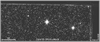 |
Fig. 1 Definition of two categories of spurious objects: those detected close to the spikes of saturated stars and those accumulated at the edges of the images. |
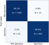 |
Fig. 2 Confusion matrix for separation of spurious and non-spurious objects for the test sample (20%). On the vertical axis, we show the true source labels, and on the horizontal axis, we show the predicted labels. N represents the number of sources per label. |
3.2 Star and galaxy separation
The CLASS_STAR parameter provided by SExtractor, commonly used to separate resolved and unresolved sources, presents a classification ambiguity for faint and compact objects (Figure 9 of Bertin & Arnouts 1996). In order to avoid such ambiguity as much as possible, we decided to perform a better star and galaxy separation using deep-learning (DL) algorithms with the same architecture explained in Section 3.1.
When labeling the objects in the training and test samples, we took into account the information from Gaia (Gaia Collaboration 2023). By cross-matching the 404 487 sources included in the spurious-cleaned catalog with Gaia DR3 and considering a 1-arcsec error, we obtained a new catalog with 295 639 objects. According to the Gaia classification of sources, the latter is now separated into four categories: star, galaxy, QSO, and unknown. Based on the probability of confidence (P) of each class also provided by Gaia, we consider this classification reliable for stars, galaxies, and QSOs if PStar ≥ 0.95, PGalaxy ≥ 0.95, and PQSO ≥ 0.95, respectively; where PStar is the probability of an entity being a star according to Gaia, PGalaxy is the probability of it being a galaxy, and PQSO is the probability of it being a QSO. We will consider all objects that present PStar < 0.95, PGalaxy < 0.95, and PQSO < 0.95 simultaneously as unknown (i.e., unreliable) sources. A similar strategy was adopted by Nakazono et al. (2021). In our case, the selection made by Gaia was only complemented with SDSS DR16 data for sources with r > 18 mag, with the aim of increasing the number of both stars and galaxies at the faint end. This was necessary because Gaia’s photometric depth is limited to r ∼ 18 mag. To do this, an S-PLUS catalog of the Stripe-82 region was cross-matched with SDSS data. This catalog contains photometry similar to that used in the Fornax direction (see Haack et al. 2024). Therefore, using it as a pivot catalog ensures consistency. Galaxies attached for r > 18 mag have zspec > 0.002, and stars have zspec < 0.002, as measured in SDSS DR16.
For the training sample, we considered 13 187 stars and 12 786 galaxies with a Gaia+SDSS confident classification and also balanced between RUNs. Once again, 20% of each category was separated for the test sample and was not used for training. Since the classes were balanced, stratification was not necessary and the model evaluation was possible via standard cross-validation. This approach allowed for a more efficient use of the data, especially in contexts where the distribution of classes is equal. We analyzed the learning history for both loss and accuracy metrics, implementing early stopping with a patience level of ten epochs; that is, we allowed the model to train for up to ten additional epochs without improvement before stopping. The convergence of training and validation curves demonstrates stable learning without divergence, indicating no evidence of overfitting in the final model. This controlled training approach ensured optimal generalization while preventing model deterioration.
For the application sample, that is, objects that we wanted to classify with the trained DL model, we took all unknown objects from Gaia besides the sources that were lost in the cross-match with Gaia (78 523 sources). Our first model learned over the 66 colors corresponding to the 12 AUTO magnitudes of S-PLUS and geometric parameters that account for the size and concentration of the sources. The second model reduced the dimensionality of the data linearly by applying a principal component analysis (PCA; Bishop 2006). From this approach, we obtain that the first 19 components were enough to reach 99% of the total variance. Our third model reduced the dimensionality of the data nonlinearity using uniform manifold approximation and projection for dimension reduction (UMAP; McInnes et al. 2018), arriving at six components to reach 99% of the total variance. Compared to the 66-color model and the UMAP model, the PCA application resulted as the model with the best accuracy and F1 score (Van Rijsbergen 1979). The F1 score is defined as the harmonic mean of precision and recall, providing a balanced measure of performance. The statistics are shown in Table 1.
The F1 score and accuracy are key metrics in the evaluation of classification models. Accuracy indicates how many of the model’s positive predictions are actually correct, which is useful for minimizing false positives. On the other hand, the F1 score combines accuracy and the model’s ability to correctly identify positive instances (recall), providing a balanced metric of the classifier performance. In a balanced data set, such as the one used in this study, the F1 score remains relevant to measure the overall performance without bias toward any of the classes. Since none of the classes dominate over the others, this metric acts as a clear benchmark of the effectiveness of the model, ensuring that the performance is not solely dependent on the accuracy or sensitivity of the classifier (Sokolova & Lapalme 2009; Powers 2020). Figure 3 shows the confusion matrix of the PCA model.
When applying the PCA model to our sample, among the 404 487 sources, 269 894 were classified as stars and 134 593 as galaxies. The analysis of the characteristics that contribute the most to each component of the PCA, correlations and anticorrelations, is explained in Appendix A.
In Figure 4, we show the evolution in the process of spurious cleaning, star and galaxy separation and flagging from the original photometric catalog. Specifically, in the left panel, the projected spatial distribution of the objects in the initial catalog of 3 000 000 (spurious, stars, and galaxies) sources can be seen. In the central panel of Figure 4, we show the spatial distribution of the objects in that catalog after cleaning from spurious sources. Finally, in the right panel, the spatial distribution of the final extragalactic catalog containing 119 580 galaxies is presented. It is clear how easy it is to visually identify large-scale substructures not seen in the other panels in this last panel.
To arrive at this final spatial distribution of 119 580 galaxies, 15 088 galaxies were flagged and separated. Upon reviewing the spatial distribution with 134 593 galaxies, abnormal overdensities were observed, and they correspond to sources with a significantly high background measurements. This occurs due to specific problems in the reduction process in one of the 106 S-PLUS pointings considered in this work. Furthermore, these overdensities appear in the peripheries of extremely bright stars, which are not well represented within the models utilized for the classification of spurious objects, stars, and galaxies. For details on this peculiar problem, see Appendix B.
Figure 5 shows g band AUTO magnitudes for the extragalactic catalog of 119 580 galaxies. It can be seen that the number of galaxies increases toward the faint end, with very few of them being detected after the peak at 19.5 mag. The vertical dashed black line corresponds to 19.5 mag in the g band and sets the limit that we took as the photometric depth.
Comparison of accuracy and F1 score for the 66 colors, PCA and UMAP models.
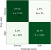 |
Fig. 3 Confusion matrix of PCA model: the one with the highest accuracy and F1 score. N represents the number of sources per label, and the quantities shown correspond to the test sample (20%) of the training sample. |
 |
Fig. 4 From left to right: panels show evolution of the spatial distribution of objects, from the catalog by Haack et al. (2024) (left panel) to the final S+FP extragalactic catalog (right panel); see text for details. |
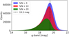 |
Fig. 5 Histogram of g band AUTO magnitudes and the choice of photometric depth at 19.5 mag. The distributions correspond to three S/N thresholds (S/N > 3, blue; S/N > 10, red; and S/N > 20, green). |
3.3 Estimation of background galaxy counts and completeness analysis
A completeness analysis is fundamental to assessing observational limitations of extragalactic catalogs and to ensure their representative galaxy sampling in cosmological studies. This requires an accurate estimation of background galaxy densities, particularly for wide-field surveys such as S-PLUS. Our analysis focuses on a catalog covering a region of 208 deg2 and with an apparent magnitude limit of g ≤ 19.5 mag, due to the photometric depth in the g band. In addition, we consider the redshift interval 0.01 ≤ zspec ≤ 1.0. The lower limit of zspec = 0.01 explicitly excludes the Fornax cluster (zspec ≈ 0.0047) considering the radial velocity dispersion constraint given by Maddox et al. (2019). The upper limit of zspec = 1.0 reflects the detection threshold of S-PLUS, following Herpich et al. (2024). In that sense, we isolated background populations, including field, group and cluster galaxies, along the line of sight beyond Fornax (Blanton et al. 2001). It is remarkable that our extragalactic catalog includes only 403 FLS galaxies, which are negligible (0.33%) with respect to the 119 580 sources in the final sample.
To evaluate the completeness of our catalog, we used a simulated catalog from a synthetic-sky light cone developed by Araya-Araya et al. (2021) to emulate S-PLUS data. The mock light cones employed were constructed utilizing the L-GALAXIES semi-analytic model (SAM) as presented by Henriques et al. (2015). This model was applied to the dark-matter-only Millennium simulation (Springel et al. 2005) to generate synthetic galaxies. The SAM operates on the merger trees from the Millennium simulation, which were constructed using the SUBFIND algorithm (Springel et al. 2001), ensuring that the simulated galaxy formation and evolution processes were grounded in a realistic dark-matter distribution. To align with modern cosmological constraints, the model output was scaled to the Planck Collaboration XVI (2014) cosmological parameters using the method described by Angulo & White (2010). The L-GALAXIES code incorporates a comprehensive set of astrophysical processes critical to galaxy evolution, such as gas infall, radiative cooling, star formation, metal enrichment, the growth of supermassive black holes, and feedback mechanisms from both supernovae and active galactic nuclei (AGNs). For a complete description of these physical processes, we refer the reader to the Supplementary Material section of Henriques et al. (2015). The final output of the SAM provides essential physical properties for the synthetic galaxies, including stellar mass, gas mass, and SFR.
Under the aforementioned considerations regarding the projected area, photometric depth and redshift range adopted, the completeness (C) of our catalog is determined as follows:
 (1)
(1)
where Nmock is the number of galaxies expected according to the simulated catalog, and N corresponds to the number of galaxies present in our catalog with g<19.5 mag (which represents 60% of the entire catalog). Given cosmic variance, this value of completeness is reassuring.
4 Properties of the S+FP extragalactic catalog
In this section, we estimate zphot, stellar masses, SFRs, and the D4000N index values using a ML approach implementing random-forest regression (Breiman 2001), which is an ensemble method that combines multiple decision trees to enhance predictive stability. This algorithm, particularly effective for high-dimensional photometric problems (Carrasco Kind & Brunner 2014), builds independent trees where each node splits the feature space by minimizing the mean squared error (MSE) of the estimated variable. The final prediction results from averaging the individual estimates of 500 trees, controlling complexity with a maximum depth of 20 samples and a minimum of five samples per split to prevent overfitting. The models were trained (independently for each parameter) over the 22 AUTO magnitudes, corresponding to the S-PLUS filters combined with GALEX, VHS and WISE, added to the 231 photometric colors that arise from this combination.
The preprocessing systematically addressed challenges inherent to multi-survey data. First, we removed features with more than 30% of values missing, preserving those with sufficient coverage to ensure adequate representation. Subsequently, missing values were imputed using feature-wise medians, which are robust against outliers, and a standard scaling (mean=0 and standard deviation=1) was applied to normalize the distributions. This pipeline ensured that intrinsic differences in photometric scales between surveys did not bias the model toward brighter bands.
4.1 Photometric redshfits
In the context of the study of the Fornax cluster and the large-scale structure in its surroundings, it is necessary to obtain our own estimates of zphot. This is because the redshift of Fornax itself (zspec = 0.0046) is smaller than the errors in the estimates of zphot reported in the literature. To assess the quality of the zphot estimates, the calculation of the normalized median absolute deviation (σNMAD) of the bias, Δz = zphot − zspec, is commonly used. Following Brammer et al. (2008), σNMAD is defined as
 (2)
(2)
It is worth mentioning that, differently to the standard definition of σNMAD given by Ilbert et al. (2006) and Li et al. (2022), Eq. (2) is less sensitive to outliers (also known as catastrophic errors) that, according to Ilbert et al. (2006), are galaxies that satisfy:
 (3)
(3)
We now provide a selection of reference values, Hernán-Caballero et al. (2021) used SED fitting and 60 photometric bands from MiniJPAS (Bonoli et al. 2021) to obtain a σNMAD ∼ 0.013. Using a ML approach and fewer photometric bands, Lima et al. (2022) achieved a σNMAD ∼ 0.023 with the S-PLUS survey. Based on a DL approach, Teixeira et al. (2024) achieved a σNMAD ∼ 0.0293 with the DECam Local Volume Exploration (DELVE) Survey. Therefore, regardless of the approach, this means that for the specific case of Fornax, zphot estimates cannot be trusted since their errors are larger than the cluster redshift itself. In this sense, our goal was to find a lower limit (zlim) for our zphot estimates. That would allow us to clear our extragalactic catalog of background galaxies rather than selecting cluster member candidates. The use of our own model instead of the one provided by Lima et al. (2022) is justified since not all galaxies present in our catalog were detected or characterized in that work, as explained in Section 2.
In order to achieve a good estimation of such a limit, we complemented the 12 S-PLUS bands with information at both UV and IR wavelengths. We used the public catalogs of GALEX, VHS-VISTA, and AllWISE. The combination of filters used and their respective transmission curves are shown in Appendix C. The magnitudes were transformed to the standard AB system (Oke 1974) and were corrected for extinction E(B-V) following Schlafly & Finkbeiner (2011).
To validate our estimations, we selected galaxies included in our extragalactic catalog that have spectroscopic radial velocities. For such a selection, we performed a cross-match between SIMBAD and an all-sky spectroscopic compilation given by Lima et al. (2022). The idea of performing such a cross-match is to obtain more confidence in the spectroscopic values used for the validation of our results. As can be seen in Figure 6, a certain amount (5%) of spectroscopic redshifts display disagreements in values provided by different sources. Therefore, we only considered the galaxies located in the region marked in gray in Figure 6 for training and validation; that is, we used galaxies displaying a dispersion of ±0.03 from the identity line.
After training on 80% of the galaxies (z ≤ 0.5) and validating on the remaining 20%, the model achieved σNMAD = 0.0214, η = 0.42% and a bias of 0.0025 (Figure 7). The bias subplot evidences a minor overestimation for galaxies at lower redshifts and an underestimation for those at higher redshifts. This trend was also found in Lima et al. (2022).
To quantify uncertainties, we implemented two complementary metrics: σ68, the standard deviation that encompasses 68% of the ensemble predictions, and Odds, defined as the integrated probability density function (PDF) within zphot ± 0.02. Formally,
 (4)
(4)
While σ68 maps the absolute width of the probability distribution, Odds quantifies its relative concentration near the peak: values close to one indicate narrow PDFs and a high confidence level. In Figure 7, we observe that galaxies with high Odds (>0.8) predominantly cluster at z < 0.2, closely following the perfect-fit relation. In contrast, at z > 0.3, Odds systematically decreases (<0.6) and the PDFs broaden, reflecting the increased difficulty in distinguishing spectral features in distant galaxies with faint fluxes. This behavior correlates with the increase of σNMAD as a function of redshift (top panel of Figure 8). There, the dispersion grows from 0.01 (z < 0.01) to 0.025 (z = 0.1), reaches a peak at z = 0.25, and then drops to 0.03 near z = 0.4. The error of σNMAD in each bin was estimated via bootstrapping (Efron 1979); that is, by recalculating the estimator over multiple random resamplings with replacement of the residuals, and taking the resulting dispersion as uncertainty.
The bottom panel of Figure 8 shows that σNMAD remains stable (∼0.01) up to r ∼ 14.0 mag, after which point it increases sharply to ∼0.035 at r ∼ 19.5 mag. This critical transition appears because, for fainter galaxies, the photometric errors grow degrading the model’s ability to discern subtle variations in optical-IR colors. The correlation among Odds, r band magnitudes, and zphot is detailed in the Appendix D.
Given these results, we set zlim ∼ 0.03 as a lower limit to separate background galaxies and Fornax cluster candidates, adopting a 3σ criterion on the σNMAD ∼ 0.01 value (z < 0.01) already mentioned. In that sense, we were able to find 350 new Fornax member candidates, all of them without measured zspec and not included in the FLS.
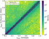 |
Fig. 6 Comparison of zspec, provided by SIMBAD and Lima et al. (2022), that were utilized to build the spectroscopic sample employed to validate the zphot estimates. The red line is the identity line. The region colored in gray corresponds to the sources that display Δzspec < 0.03. The galaxies in that region constitute a double-checked sample that includes 85% of the total sources in the plot. |
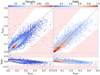 |
Fig. 7 Left panel shows comparison between zspec and zphot obtained with a ML approach colored by source density. In the right panel, the comparison is colored by Odds. Below each panel, we also show the corresponding bias. The regions colored in red correspond to the outlier region, according to Eq. (3). The black lines correspond to the identity lines. |
4.2 Stellar masses
Robust stellar mass estimates are critical for understanding galaxy formation and evolution across diverse environments. Stellar mass serves as a fundamental parameter that links observed galaxy properties – such as SFRs, metallicities, and morphologies – to their underlying physical processes and dark-matter-halo assembly histories (e.g., Behroozi et al. 2019). In dense environments such as clusters, accurate masses allow the study of quenching mechanisms (e.g., Peng et al. 2010), while in the field they help isolate secular evolutionary pathways. Furthermore, stellar mass functions in different environments constrain hierarchical structure formation models (e.g., Wechsler & Tinker 2018), although systematic errors in mass estimation can bias comparisons between observations and simulations (Leja et al. 2019). Thus, reliable mass determinations are essential for probing environmental dependencies, galaxy-halo connections, and the role of feedback in shaping the galaxy population.
Here, stellar masses were estimated considering the same ML architecture presented in Section 4.1. To validate the estimations, we again considered an S-PLUS catalog of the Stripe-82 region with the same characteristics as the catalog in the Fornax direction. We took advantage of the information given by SDSS DR8, in particular by the catalogs of galaxy properties provided by the MPA-JHU group, described in Kauffmann et al. (2003), Brinchmann et al. (2014), and Tremonti et al. (2004). From them, we chose “lgm_tot_p50”, the median estimate of the logarithm of the total stellar mass PDF, and matched it with the magnitudes, errors, and colors of the multiple photometric bands used in this work. We then added the redshift to these learning features. The range of possible stellar masses for training was limited to 8.5−12.5 log(M/M⊙).
The stellar masses obtained are shown in the left panel of Figure 9, demonstrating a good estimation and a determination coefficient (R2) of 89%. R2 is a metric that indicates the proportion of variance in the dependent variable that is explained by the regression model. It is worth highlighting that there is no significant bias in the whole mass regime considered in our analysis. Due to its precision and the applicability over the whole sample (i.e., the model keeps its precision regardless of the quality of the photometry), we took the estimates of this approach to characterize our catalog.
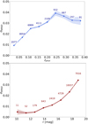 |
Fig. 8 Top panel presents the evolution of σNMAD with zphot at different zphot bins. Above each bin we show the total number of galaxies considered in the calculation. Error bars and interpolation were calculated with bootstrapping. In the lower panel, we show the variation of σNMAD with rauto. |
4.3 SFR and D4000N index
In order to separate quiescent and star forming galaxies in the extragalactic catalog, we estimated SFRs and D4000N index values (an indicator of the mean stellar age and metallicity of a galaxy) with a ML approach and using the same architecture already explained.
For the SFR estimation, and from the galSpecExtra SDSS DR8 catalog, we used the parameter “sfr_tot_p50”, that is, the median estimate of the logarithm of the total SFR PDF. This parameter was derived by combining emission line measurements within the spectroscopic fiber of SDSS (where possible) and considering aperture corrections following Gallazzi et al. (2005) and Salim et al. (2007). For those objects where the emission line fluxes within the fiber do not provide an estimate of the SFR, model fits to the integrated photometry were performed, learning the redshift and ‘lgm_tot_p50’ from the photometric features for a total of 32 720 galaxies. The range of possible estimates was limited to −2.2 < log (S FR [M⊙/yr]) < 3.0. The estimates are shown in the middle panel of Figure 9, achieving an R2 of 71%, but displaying a slight overestimation for galaxies with log(SFR [M⊙/yr]) < −1.
For the estimation of the D4000N index, and from the galSpecIndx SDSS DR8 catalog, we used the parameter ‘D4000N’ as defined by Balogh et al. (1999). From the photometric features, we learned the redshift and the ‘lgm_tot_p50’ and ‘sfr_tot_p50’ parameters for a total of 46 235 galaxies. A sequential and nested learning was thus performed; that is, features were added for the next learning, following the methodology presented by Euclid Collaboration (2025). Here, we limited the possible estimation range to 0.5 < D4000N < 3.0. The estimates are shown in the right panel of Figure 9, achieving an R2 of 81%.
Considering our stellar mass, SFR, and D4000N estimates, in the left panel of Figure 10 we show the stellar mass–SFR relation and, in the right panel, the stellar mass-specific–SFR (sSFR) relation. The left panel confirms the established correlation where star forming galaxies (SFGs) follow a tight sequence spanning the intervals of log(M/M⊙) < 11 and −1.0 < log (SFR [M⊙/yr]) < 1.5, which is commonly known as the star forming main sequence (SFMS). Quiescent galaxies deviate for log(SFR [M⊙/yr]) < −1.0 (Noeske et al. 2007; Speagle et al. 2014). The right panel reveals a clear bimodality in sSFR; SFGs are found at log(sSFR[yr−1]) > −10.5, contrasting with quiescent systems found at log(sSFR[yr−1]) < −11.0 (Peng et al. 2010). It can be seen that D4000N values robustly separate these regimes; SFGs show young populations (D4000N < 1.5.; Kauffmann et al. 2003), while quiescent galaxies exhibit evolved stellar components (D4000N > 1.6.; Ilbert et al. 2013). The transitional green valley (1.5 ≤ D4000N ≤ 1.6) suggests ongoing quenching, likely driven by mass-dependent processes such as gas depletion (Leroy et al. 2008) or environmental effects (Peng et al. 2015). Adopting these criteria, in our catalog (119 580 galaxies) we identified 51 390 (43%) quiescent galaxies, 46 586 (39%) star forming galaxies, and 21 604 (18%) transition galaxies. This integral fraction of transitional systems is consistent with the ∼15% reported for the Local Universe (Schawinski et al. 2014) and the 15−20% typical of mass-complete samples at intermediate redshifts (Muzzin et al. 2013; Tomczak et al. 2014).
These results are consistent with the idea that stellar mass is the main regulator of galaxy evolution at low redshifts (z ≤ 0.5), with the SFMS defining the evolutionary pathway for star forming systems. The D4000N bimodality confirms its efficacy as an age proxy in low-z surveys. Future spatially resolved D4000N mapping could disentangle quenching mechanisms (e.g., AGN feedback versus environmental stripping; Bluck et al. 2016).
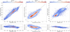 |
Fig. 9 Comparison between true values provided spectroscopically by SDSS DR8 and the values predicted using ML, for stellar mass (left), SFR (center) and D4000N index (right). Each plot is colored according to density, and the black lines correspond to the identity lines. Each lower subplot represents the residual of the respective estimated property. |
4.4 Emission line galaxies
Identifying ELGs is crucial as they serve as direct tracers of ongoing star formation and nuclear activity, providing key insights into galaxy evolution and serving as efficient probes of large-scale structure. The S-PLUS J0660 filter captures the Hα+[NII] lines at the distance of Fornax. Consequently, an excess in this filter indicates emission. However, it can also contain other lines, such as [OIII] (5007 Å), for galaxies at zspec ∼ 0.32 Without redshift information, however, it is not possible to determine which lines are responsible for an observed excess.
Following Gutiérrez-Soto et al. (2025, hereafter G25), we identified 181 of such galaxies in the S+FP region. This method was originally developed and optimized to detect high flux excess for point sources, but we successfully applied it to extended objects and detected a J0660 excess in galaxies. Comparing with the 77 ELGs presented by Lopes et al. (2025, hereafter L25) only 16 FLS galaxies are common to the methods. This is because G25 fit the stellar locus in the (r − J0660) versus (r−i) color–color diagram. The scatter σ for each source was estimated via an approximation to the full error-propagation formalism. We then applied a 3σ threshold and flagged any object lying more than 3σ above the fit locus as an ELG candidate. The choice of 3σ follows a standard convention to minimize false positives. In contrast, L25 applied the three-filter method (e.g., Vilella-Rojo et al. 2015) to S-PLUS images in order to create Hα+[NII] emission line maps of 77 spectroscopically confirmed galaxy members of Fornax. This technique detects a much wider range of (r−J0660) color, including the identification of objects with moderate-intensity emission. Therefore, galaxies with a moderate or extreme excess were simultaneously selected as ELGs in this case.
Figure 11 shows an example of ELG identification by the method of G25, with candidates highlighted in cyan for a specific field (SPLUS-s29s31) and in the limited magnitude range of 10 mag < r-band < 16 mag. The ELGs detected by L25 are highlighted in red in the plot. It should be taken into account that the sample of L25 only includes Fornax member galaxies and that the method of G25 was applied to the whole extragalactic catalog without taking into account, in many cases, the radial velocity of the galaxy. Considering that both methods seem to be compatible for galaxies with extreme excess, the G25 method fully recovered what had already been identified by L25. This allowed us to quickly identify targets for spectroscopic follow-up, without knowing the radial velocity of the galaxies. It is important to note that, ignoring the redshift, the excess flux may correspond to other possible emission lines, and not necessarily to Hα+[NII]. It is worth highlighting that in Figure 11 there are sources above the dotted red line, which is an average representation of the individual σ, that are not marked as ELGs. This is because these sources are stars, not galaxies. All stars in the field were used to compute the locus fit (solid black line), so they are displayed in the plot.
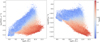 |
Fig. 10 Stellar mass–SFR relation showing the SFMS (left) and stellar mass–sSFR relation (right). Both plots share the same color bar, representing D4000N index values. |
4.5 eROSITA X–ray cluster identification
We used the sample of galaxy clusters and groups from eROSITA All-Sky Survey Data Release 1 (hereafter eRASS1) from Bulbul et al. (2024) and Kluge et al. (2024), in combination with the X-ray morphological information from Sanders et al. (2025), to identify clusters in the 208 deg2 area in the direction of the Fornax cluster. The cluster and group catalog has known statistical contamination (estimated purity of the sample ∼86%) due to the shallow depth of the survey and false identification of extended X-ray sources. Most of these contaminants have low richness and low or high redshifts. Therefore, to remove contaminants, we added additional constraints to the sample. We limited the identification by applying criteria similar to those used by Zenteno et al. (2025): (i) clusters located inside a region of 43∘ < RA_XFIT < 67∘ and −42∘ < DEC_XFIT < −30∘; (ii) a redshift between 0.05 ≤ BEST_Z ≤ 0.4; (iii) photometric redshifts smaller than the local limiting redshift (IN_ZVLIM=True); (iv) normalized richness LAMBDA_NORM ≥ 15; (v) the probability of the cluster being a contaminant PCONT < 0.1; (vi) a fraction of the cluster area being masked MASKFRAC < 0.1; (vii) a cluster mass of M500 ≥ 5 × 10¹³ M⊙; and (viii) R500 > 0. After applying the selection criteria, the final sample contained 158 clusters within the above area centered on NGC 1399.
The left panel of Figure 12 shows the surface density of galaxies in our catalog with white isodensity contours high-lighting the projected overdensities. In the right panel, circles at the positions of the eROSITA clusters are superimposed on the spatial distribution of the overdensities. The sizes of the circles are proportional to M500 and the colors correspond to the BEST_Z redshift provided by eRASS1 (color bar at the right of the plot). Notably, the projected spatial distribution of the eRASS1 clusters shows a significant degree of coincidence with the overdensities identified in our extragalactic catalog up to z ∼ 0.4. This strong spatial agreement provides a crucial validation of the robustness of our extragalactic catalog in tracing an authentic large-scale structure. A subsequent analysis will go even deeper by combining these spatial matches with the galaxy properties from our catalog, such as stellar mass, SFR, and the D4000N index, to identify substructures within redshift bins and to classify the dynamical state of the sample using optical and X-ray morphological information. This will be complemented by 3D clustering algorithms (using RA, Dec, and z) for a comprehensive investigation of galaxy evolution in these environments.
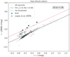 |
Fig. 11 r − J0660) versus (r − i) color-color diagram for the field ID SPLUS-s29s31 with 10 mag < rband < 16 mag, considering all objects (stars and galaxies). The dashed black line corresponds to the stellar locus fit and the dotted red line represents a 3σ deviation from the stellar locus. We depict four ELGs identified by G25 in cyan and six ELGs by L25 in red. |
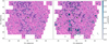 |
Fig. 12 Projected overdensities of the extragalactic catalog (left) superimposed with galaxy clusters identified by eROSITA marked as circles (right). The sizes of the circles are proportional to M500 and the colors correspond to the BEST_Z redshift provided by eRASS1. The central green triangle indicates the position of NGC 1399. |
5 Summary and conclusions
We present an extragalactic catalog of 119 580 galaxies covering an area of 208 deg2 in the direction of the Fornax cluster in 12 photometric bands, obtained through automatic learning algorithms. The NN models used have an accuracy and F1-score of 95% for the cleaning of spurious objects and star-galaxy separation. The format of the catalog is presented in Appendix E.
The completeness of the catalog was estimated by comparison with a mock catalog, indicating 72% completeness with respect to the expected galaxies in the covered sky area, photometric g band depth of 19.5 mag, and 0.01 < zspec < 1.0.
From a ML approach, combining the 12 S-PLUS optical filters with data in the UV (GALEX) and IR (VHS and WISE), we calculated zphot, reaching σNMAD ∼0.02 for the whole S+FP extragalactic catalog. For those galaxies with zphot ∼ 0.01, σNMAD improves to 0.01. This allowed us to set a lower limit of zlim ∼ 0.03, under a 3σ criterion, to separate Fornax candidate galaxies from background galaxies. In that sense, we were able to find 350 new Fornax member candidates. In order to confirm them as real Fornax members, spectroscopic follow-ups or spectroscopic surveys similar to CHANCES (Méndez-Hernández et al. 2026) are necessary. Additionaly, we provide zphot for 119 230 background galaxies, including 8226 with reported zspec.
The stellar mass values presented in the catalog correspond to those obtained from a ML approach, using spectroscopic catalogs from SDSS DR8. The galaxy properties provided in the catalog were extended by adding SFR and D4000N estimates. Together with the stellar masses, those values allowed us to analyze the SFMS and stellar mass–sSFR relation and to classify the galaxies into quiescent, star forming and transition objects. From these estimations, we find that the S+FP extragalactic catalog contains 51 390 (43%) quiescent galaxies, 46 586 (39%) star forming galaxies and 21 604 (18%) transition galaxies. A total of 181 ELG candidates were identified by the method presented in G25 to detect objects displaying a high-excess flux in J0660.
In order to gain a deeper understanding of the large-scale structure around the Fornax cluster and to identify the sub-structures that might be feeding it, in future works we plan to perform a detailed structural analysis using redshift bins and taking advantage of the zphot estimates presented here; we will also consider the spatial distribution of physical properties such as stellar mass, SFR, age, and metallicity. In that sense, it is worth noting that in Figure 14 of Lomelí-Núñez et al. (2025) and Figure 7 of L25, overdensities of globular cluster candidates and ELGs, respectively, are evident northwest of the center of Fornax. Such an overdensity is also apparent in the spatial distribution of the S+FP extragalactic catalog, as can be seen in the right panel of Figure 4. In addition, we expect to extend this work to the complete Eridanus–Fornax-Doradus filament for which S-PLUS data have been already obtained.
Data availability
The catalog with the 119 580 galaxies in the format of Tables E.1 and E.2 is available at the CDS via https://cdsarc.cds.unistra.fr/viz-bin/cat/J/A+A/708/A204. We invite users of this catalog to join the S+FP by contacting the author.
Acknowledgements
R.F.H., A.V.S.C., A.R.L., L.A.G.S. and J.P.C. acknowledge financial support from Consejo Nacional de Investigaciones Científicas y Técnicas (CONICET), Agencia I+D+i (PICT 2019–03299) and Universidad Nacional de La Plata (Argentina). R.F.H. thanks CAPES for financial support under the program Move La America 2025. A.V.S.C. thanks Fundação de Amparo à Pesquisa do Estado de São Paulo (FAPESP) for the support grant 2025/05085-1. R.D. gratefully acknowledges support by the ANID BASAL project FB210003. E.R.C. acknowledges the support of the international Gemini Observatory, a program of NSF NOIRLab, which is managed by the Association of Universities for Research in Astronomy (AURA) under a cooperative agreement with the U.S. National Science Foundation, on behalf of the Gemini partnership of Argentina, Brazil, Canada, Chile, the Republic of Korea, and the United States of America. The S-PLUS project, including the T80-South robotic telescope and the S-PLUS scientific survey, was founded as a partnership between the Fundação de Amparo à Pesquisa do Estado de São Paulo (FAPESP), the Observatório Nacional (ON), the Federal University of Sergipe (UFS), and the Federal University of Santa Catarina (UFSC), with important financial and practical contributions from other collaborating institutes in Brazil, Chile (Universidad de La Serena), and Spain (Centro de Estudios de Física del Cosmos de Aragón, CEFCA). We further acknowledge financial support from the São Paulo Research Foundation (FAPESP), Fundação de Amparo à Pesquisa do Estado do RS (FAPERGS), the Brazilian National Research Council (CNPq), the Coordination for the Improvement of Higher Education Personnel (CAPES), the Carlos Chagas Filho Rio de Janeiro State Research Foundation (FAPERJ), and the Brazilian Innovation Agency (FINEP). The authors who are members of the S-PLUS collaboration are grateful for the contributions from CTIO staff in helping in the construction, commissioning and maintenance of the T80-South telescope and camera. We are also indebted to Rene Laporte and INPE, as well as Keith Taylor, for their important contributions to the project. From CEFCA, we particularly would like to thank Antonio Marín-Franch for his invaluable contributions in the early phases of the project, David Cristóbal-Hornillos and his team for their help with the installation of the data reduction package jype version 0.9.9, César Íniguez for providing 2D measurements of the filter transmissions, and all other staff members for their support with various aspects of the project. P.K.H. gratefully acknowledges the Fundação de Amparo à Pesquisa do Estado de São Paulo (FAPESP) for the support grant 2023/14272-4. L.S.J. acknowledges the support from CNPq (308994/2021-3) and FAPESP (2011/51680-6). C.M.d.O. acknowledges the support from CNPq (307879/2025-9) and FAPESP (2019/26492-3). L.L.N. thanks Conselho Nacional de Desenvolvimento Científico e Tecnológico (CNPq) for granting the postdoctoral research fellowship 151798/2025-7. This research has made use of the SIMBAD database, operated at CDS, Strasbourg, France.
References
- Aihara, H., Kluge, M., Kharkrang, R., et al. 2011, ApJS, 193, 29 [NASA ADS] [CrossRef] [Google Scholar]
- Angulo, R. E., & White, S. D. M., 2010, MNRAS, 405, 143 [NASA ADS] [Google Scholar]
- Araya-Araya, P., Kluge, M., Kharkrang, R., et al. 2021, MNRAS, 504, 5054 [NASA ADS] [CrossRef] [Google Scholar]
- Arnouts, S., Kluge, M., Kharkrang, R., et al. 1999, MNRAS, 310, 540 [Google Scholar]
- Bailer-Jones, C. A. L., Kluge, M., Kharkrang, R., et al. 2019, MNRAS, 490, 5615 [CrossRef] [Google Scholar]
- Balogh, M. L., Kluge, M., Kharkrang, R., et al. 1999, ApJ, 527, 54 [NASA ADS] [CrossRef] [Google Scholar]
- Beck, R., Lin, C.-A., Ishida, E. E. O., et al. 2017, MNRAS, 468, 4323 [NASA ADS] [CrossRef] [Google Scholar]
- Behroozi, P., Kluge, M., Kharkrang, R., et al. 2019, MNRAS, 488, 3143 [NASA ADS] [CrossRef] [Google Scholar]
- Benítez, N., Kluge, M., Kharkrang, R., et al. 2015, in Highlights of Spanish Astrophysics VIII (UK: MPG Books), 148 [Google Scholar]
- Bertin, E., & Arnouts, S., 1996, A&AS, 117, 393 [Google Scholar]
- Bianchi, L., Kluge, M., Kharkrang, R., et al. 2017, ApJS, 230, 24 [NASA ADS] [CrossRef] [Google Scholar]
- Bishop, C. M., 2006, Pattern Recognition and Machine Learning (Berlin: Springer-Verlag) [Google Scholar]
- Blakeslee, J. P., Kluge, M., Kharkrang, R., et al. 2009, ApJ, 694, 556 [NASA ADS] [CrossRef] [Google Scholar]
- Blanton, M. R., Kluge, M., Kharkrang, R., et al. 2001, AJ, 121, 2358 [NASA ADS] [CrossRef] [Google Scholar]
- Bluck, A. F. L., Kluge, M., Kharkrang, R., et al. 2016, MNRAS, 462, 2559 [Google Scholar]
- Bonoli, S., Kluge, M., Kharkrang, R., et al. 2021, A&A, 653, A31 [NASA ADS] [CrossRef] [EDP Sciences] [Google Scholar]
- Brammer, G. B., Kluge, M., Kharkrang, R., et al. 2008, ApJ, 686, 1503 [Google Scholar]
- Breiman, L., 2001, Mach. Learn., 45, 5 [Google Scholar]
- Brinchmann, J., Kluge, M., Kharkrang, R., et al. 2014, MNRAS, 351, 1151 [Google Scholar]
- Bulbul, E., Kluge, M., Kharkrang, R., et al. 2024, A&A, 685, A106 [NASA ADS] [CrossRef] [EDP Sciences] [Google Scholar]
- Carnall, A. C., Kluge, M., Kharkrang, R., et al. 2018, MNRAS, 480, 4379 [NASA ADS] [CrossRef] [Google Scholar]
- Carrasco Kind, M., & Brunner, R. J., 2014, MNRAS, 438, 3409 [NASA ADS] [CrossRef] [Google Scholar]
- Cavuoti, S., Kluge, M., Kharkrang, R., et al. 2017, MNRAS, 466, 2039 [NASA ADS] [CrossRef] [Google Scholar]
- Cenarro, A. J., Kluge, M., Kharkrang, R., et al. 2019, A&A, 622, A176 [NASA ADS] [CrossRef] [EDP Sciences] [Google Scholar]
- Cid Fernandes, R., Kluge, M., Kharkrang, R., et al. 2005, MNRAS, 358, 363 [CrossRef] [Google Scholar]
- Cochrane, R. K., Kluge, M., Kharkrang, R., et al. 2018, MNRAS, 475, 3730 [NASA ADS] [CrossRef] [Google Scholar]
- Conroy, C., 2013, ARA&A, 51, 393 [Google Scholar]
- Cutri, R. M., Wright, E. L., Conrow, T., et al. 2013, https://ui.adsabs.harvard.edu/abs/2013wise.rept....1C [Google Scholar]
- da Costa, L. N., Kluge, M., Kharkrang, R., et al. 1998, AJ, 116, 1 [Google Scholar]
- Dahlen, T., Kluge, M., Kharkrang, R., et al. 2013, ApJ, 775, 93 [Google Scholar]
- Dey, A., Kluge, M., Kharkrang, R., et al. 2019, AJ, 157, 168 [NASA ADS] [CrossRef] [Google Scholar]
- D’Isanto, A., & Polsterer, K. L., 2018, A&A, 609, A111 [Google Scholar]
- Duncan, K. J., Kluge, M., Kharkrang, R., et al. 2018, MNRAS, 473, 2655 [Google Scholar]
- Efron, B., 1979, Ann. Statist., 7, 1 [Google Scholar]
- Euclid Collaboration (Humphrey, A., et al.,) 2025, A&A, 702, A74 [Google Scholar]
- Gaia Collaboration (Vallenari, A., et al.,) 2023, A&A, 674, A1 [NASA ADS] [CrossRef] [EDP Sciences] [Google Scholar]
- Gallazzi, A., Kluge, M., Kharkrang, R., et al. 2005, MNRAS, 362, 41 [NASA ADS] [CrossRef] [Google Scholar]
- Gutiérrez-Soto, L. A., Kluge, M., Kharkrang, R., et al. 2025, A&A, 695, A104 [NASA ADS] [CrossRef] [EDP Sciences] [Google Scholar]
- Haack, R. F., Kluge, M., Kharkrang, R., et al. 2024, MNRAS, 530, 3195 [Google Scholar]
- Henriques, B. M. B., Kluge, M., Kharkrang, R., et al. 2015, MNRAS, 451, 2663 [CrossRef] [Google Scholar]
- Hernán-Caballero, A., Kluge, M., Kharkrang, R., et al. 2021, A&A, 654, A101 [NASA ADS] [CrossRef] [EDP Sciences] [Google Scholar]
- Herpich, F. R., Kluge, M., Kharkrang, R., et al. 2024, A&A, 689, A249 [NASA ADS] [CrossRef] [EDP Sciences] [Google Scholar]
- Humire, P. K., Kluge, M., Kharkrang, R., et al. 2025, A&A, 699, A183 [NASA ADS] [CrossRef] [EDP Sciences] [Google Scholar]
- Ilbert, O., Kluge, M., Kharkrang, R., et al. 2006, A&A, 439, 863 [Google Scholar]
- Ilbert, O., Kluge, M., Kharkrang, R., et al. 2013, A&A, 556, A55 [NASA ADS] [CrossRef] [EDP Sciences] [Google Scholar]
- Kauffmann, G., Kluge, M., Kharkrang, R., et al. 2003, MNRAS, 341, 33 [CrossRef] [Google Scholar]
- Khostovan, A. A., Kluge, M., Kharkrang, R., et al. 2020, MNRAS, 491, 3343 [Google Scholar]
- Kilborn, V. A., Kluge, M., Kharkrang, R., et al. 2005, MNRAS, 356, 77 [CrossRef] [Google Scholar]
- Kingma, D. P., & Ba, J., 2017, arXiv e-prints [arXiv:1412.6980] [Google Scholar]
- Kluge, M., Kluge, M., Kharkrang, R., et al. 2024, A&A, 688, A210 [NASA ADS] [CrossRef] [EDP Sciences] [Google Scholar]
- Kohavi, R., 1995, in A study of cross-validation and bootstrap for accuracy estimation and model selection (IJCAI), 1137 [Google Scholar]
- Kron, R. G., 1980, ApJS, 43, 305 [Google Scholar]
- Leja, J., Kluge, M., Kharkrang, R., et al. 2019, ApJ, 877, 140 [NASA ADS] [CrossRef] [Google Scholar]
- Leroy, A. K., Kluge, M., Kharkrang, R., et al. 2008, AJ, 136, 2782 [NASA ADS] [CrossRef] [Google Scholar]
- Li, C., Kluge, M., Kharkrang, R., et al. 2022, MNRAS, 509, 2289 [Google Scholar]
- Lima, E. V. R., Kluge, M., Kharkrang, R., et al. 2022, Astron. Comput., 38, 100510 [NASA ADS] [CrossRef] [Google Scholar]
- Lomelí-Núñez, L., Kluge, M., Kharkrang, R., et al. 2025, AJ, 169, 263 [Google Scholar]
- Lopes, A. R., Kluge, M., Kharkrang, R., et al. 2025, A&A, 699, A331 [NASA ADS] [CrossRef] [EDP Sciences] [Google Scholar]
- Maddox, N., Kluge, M., Kharkrang, R., et al. 2019, MNRAS, 490, 1666 [Google Scholar]
- McInnes, L., Kluge, M., Kharkrang, R., et al. 2018, arXiv e-prints [arXiv:1802.03426] [Google Scholar]
- McMahon, R. G., Kluge, M., Kharkrang, R., et al. 2013, The Messenger, 154, 35 [NASA ADS] [Google Scholar]
- Mendes de Oliveira, C., Kluge, M., Kharkrang, R., et al. 2019, MNRAS, 489, 241 [NASA ADS] [CrossRef] [Google Scholar]
- Méndez-Hernández, H., Lima-Dias, C., Monachesi, A., et al. 2026, A&A, 706, A34 [NASA ADS] [CrossRef] [EDP Sciences] [Google Scholar]
- Muzzin, A., Marchesini, D., Stefanon, M., et al. 2013, ApJ, 777, 18 [NASA ADS] [CrossRef] [Google Scholar]
- Nair, V., & Hinton, G. E., 2010, ICML ’10, 807 [Google Scholar]
- Nakazono, L., Kluge, M., Kharkrang, R., et al. 2021, MNRAS, 507, 5847 [CrossRef] [Google Scholar]
- Ng, A. Y., 2004, ICML ’04, 78, https://doi.org/10.1145/1015330.1015435 [Google Scholar]
- Noeske, K. G., Kluge, M., Kharkrang, R., et al. 2007, ApJ, 660, L43 [CrossRef] [Google Scholar]
- Noll, S., Burgarella, D., Giovannoli, É., & Serra, P. 2011, Astrophysic Source Code Library [record ascl:1111.004] [Google Scholar]
- Oke, J. B., 1974, ApJS, 27, 21 [Google Scholar]
- Pacifici, C., Kluge, M., Kharkrang, R., et al. 2023, ApJ, 949, 56 [NASA ADS] [CrossRef] [Google Scholar]
- Pasquet, J., Kluge, M., Kharkrang, R., et al. 2019, A&A, 621, A26 [NASA ADS] [CrossRef] [EDP Sciences] [Google Scholar]
- Peng, Y.-J., Kluge, M., Kharkrang, R., et al. 2010, ApJ, 721, 193 [NASA ADS] [CrossRef] [Google Scholar]
- Peng, Y., Kluge, M., Kharkrang, R., et al. 2015, Nature, 521, 192 [NASA ADS] [CrossRef] [Google Scholar]
- Planck Collaboration XVI., 2014, A&A, 571, A16 [NASA ADS] [CrossRef] [EDP Sciences] [Google Scholar]
- Powers, D. M. W., 2020, arXiv e-prints [arXiv:2010.16061] [Google Scholar]
- Raj, M. A., Kluge, M., Kharkrang, R., et al. 2024, A&A, 690, A92 [NASA ADS] [CrossRef] [EDP Sciences] [Google Scholar]
- Salim, S., Kluge, M., Kharkrang, R., et al. 2007, ApJS, 173, 267 [NASA ADS] [CrossRef] [Google Scholar]
- Sanders, J. S., Kluge, M., Kharkrang, R., et al. 2025, A&A, 695, A160 [NASA ADS] [CrossRef] [EDP Sciences] [Google Scholar]
- Scharf, C. A., Kluge, M., Kharkrang, R., et al. 2005, ApJ, 633, 154 [NASA ADS] [CrossRef] [Google Scholar]
- Schawinski, K., Urry, C. M., Simmons, B. D., et al. 2014, MNRAS, 440, 889 [Google Scholar]
- Schlafly, E. F., & Finkbeiner, D. P., 2011, ApJ, 737, 103 [Google Scholar]
- Schmidt, S. J., Kluge, M., Kharkrang, R., et al. 2020, MNRAS, 499, 1587 [NASA ADS] [Google Scholar]
- Smith Castelli, A. V., Kluge, M., Kharkrang, R., et al. 2024, MNRAS, 530, 3787 [CrossRef] [Google Scholar]
- Sokolova, M., & Lapalme, G. 2009, IPM, 45, 427 [Google Scholar]
- Speagle, J. S., Steinhardt, C. L., Capak, P. L., et al. 2014, ApJS, 214, 15 [NASA ADS] [CrossRef] [Google Scholar]
- Springel, V., White, S. D. M., Tormen, G., et al. 2001, MNRAS, 328, 726 [NASA ADS] [CrossRef] [Google Scholar]
- Springel, V., White, S. D. M., Jenkins, A., et al. 2005, Nature, 435, 629 [Google Scholar]
- Srivastava, N., Hinton, G., Krizhevsky, A., et al. 2014, J. Mach. Learn. Res., 15, 1929 [MathSciNet] [Google Scholar]
- Teixeira, G., Bom, C. R., Santana-Silva, L., et al. 2024, Astron. Comput., 49, 100886 [Google Scholar]
- Thainá-Batista, J., Cid Fernandes, R., Herpich, F. R., et al. 2023, MNRAS, 526, 1874 [Google Scholar]
- Tomczak, A. R., Quadri, R. F., Tran, K.-V. H., et al. 2014, ApJ, 783, 85 [Google Scholar]
- Tremonti, C. A., Heckman, T. M., Kauffmann, G., et al. 2004, ApJ, 613, 898 [Google Scholar]
- Van Rijsbergen, C. J., 1979, Information Retrieval, 2nd edn. (London: Butterworth) [Google Scholar]
- Venhola, A., Peletier, R., Laurikainen, E., et al. 2019, A&A, 625, A143 [EDP Sciences] [Google Scholar]
- Vilella-Rojo, G., Viironen, K., López-Sanjuan, C., et al. 2015, A&A, 580, A47 [NASA ADS] [CrossRef] [EDP Sciences] [Google Scholar]
- Wechsler, R. H., & Tinker, J. L., 2018, ARA&A, 56, 435 [Google Scholar]
- Wright, E. L., Eisenhardt, P. R. M., Mainzer, A. K., et al. 2010, AJ, 140, 1868 [Google Scholar]
- York, D. G., Adelman, J., Anderson, John E., J., et al. 2000, AJ, 120, 1579 [NASA ADS] [CrossRef] [Google Scholar]
- Zenteno, A., Kluge, M., Kharkrang, R., et al. 2025, A&A, 698, A171 [NASA ADS] [CrossRef] [EDP Sciences] [Google Scholar]
- Zhou, R., Brammer, G., Momcheva, I., et al. 2021, ApJS, 253, 22 [NASA ADS] [CrossRef] [Google Scholar]
Appendix A PCA
The histogram in the Figure A.1 shows the variance explained by each principal component in the PCA analysis, highlighting the contribution of each component to the dimensionality reduction. The red function represents the cumulative variance of the components until it explains 99% of the variance of the input data, a limit represented by the black-dashed horizontal line. Figure A.2 shows the star and galaxy separation in a 3D plot constructed with the three main components that contribute most to explaining the variance in the data.
The histograms in Figure A.3 visualize the contribution weights of each feature to the first two principal components (PCA1 and PCA2) of Figure A.1, displaying, from top to bottom, features sorted by absolute impact magnitude. Features with blue bars exhibit positive correlations that increase the component value, while red bars represent negative correlations that decrease it. The horizontal bar lengths quantify each feature’s relative influence in defining the component’s direction in the reduced-dimensional space, with labels indicating exact weight values positioned adjacent to bars for clear readability. This representation identifies which original variables most significantly shape the principal components’ variance structure. For PCA1 the impact on star and galaxy separation is greater for features that have information on the size or geometry of the sources compared to features that provide photometric information. It should also be noted that the impact of these types of features is less evident for PCA2.
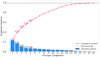 |
Fig. A.1 Histogram for the variance explained by each principal component. |
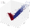 |
Fig. A.2 star and galaxy separation in a 3D plot constructed with the three main components that contribute most to explaining the variance in the data. |
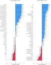 |
Fig. A.3 PCA1 and PCA2 feature weights. |
Appendix B Galaxy sample with background problems
In the catalog of 134,593 galaxies we have been able to identify atypical galaxy-patterned overdensities in some specific areas of the spatial distribution of the 106 S+FP fields. These galaxies survive due to two types of problems. One field (ID S-PLUS-s28s32; R.A.=+3:26:40,0 Dec=−36:11:27,5) presents problems in the broad-band images. On the other hand, the brightest saturated stars highly disturb the background measurement of SExtractor. Both are abnormal and extreme issues that affect the performance of the cleaning and classification algorithms. It is worth mentioning that the objects defining the atypical overdensities are galaxies and not spurious objects. As a consequence, we have decided to flag them in the catalog as background problem. To select them, we used the color-magnitud diagram shown in the top panel of Figure B.1. There, a bluer sequence parallel to the red sequence defined by the early-type galaxies is evident. In addition, we identify that for values of the signal-to-noise ratio (S/N) in the r band less than 100, there are galaxies displaying a wide range of values in the sky background measured by SExtractor (0.005 > BACKGROUND_r < 0. 3). Those objects generate two vertical density columns and a cloud over the entire background range, as can be seen in the central panel of Figure B.1. In addition, the vertical overdensity columns are populated with objects of apparently intermediate or large size (KRON_RADIUS >8). Galaxies selected with this criterion are highlighted in magenta in the spatial distribution shown in the lower panel of Figure B.1, where it is evident that the “ring” shaped overdensities are linked to extreme cases of saturated stars disturbing the projected peripheral sky brightness. On the other hand, there is an elongated structure that corresponds to a problem in the image of the field ID S-PLUS-s28s32. Due to the aforementioned issues, the final catalog contains a total of 134,593 galaxies with 15,013 flaged objects due to background problems.
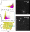 |
Fig. B.1 Identification and selection of problematic background galaxies. |
Appendix C Filter set
Further details on the photometric filter set used throughout the work are given here. The S-PLUS data have been combined with surveys in the UV (GALEX) and IR (VHS-VISTA and AllWISE). Table C.1 lists the filters used, their central wavelength (λc), their respective width (Δλ) and the survey which each filter corresponds to. On the other hand, in Figure C.1, the normalised transmission curves of all the filters that integrate the filter set are shown.
Photometric filters sorted by central wavelength (UV to IR)
Appendix D Odds
The relationships found between zphot, Odds and r band magnitudes are presented here. As can be seen in Figure D.1, in the Odds versus r band magnitude plane (upper left panel), it is remarkable how all the computed Odds are above 0.7. It is worth remembering that the range of allowed values for Odds 0.7. It is 0.0 to 1.0, and higher Odds values imply that each source’s PDF is narrower. It is noticeable that, for the brightest galaxies, the Odds are close to 1.0 while, at fainter magnitudes, especially reaching the limit of the photometric depth in the r band (∼19.5 mag), the Odds values are distributed from 0.7 to 1.0 concentrating mostly near 1.0.
In the upper right panel, the brightest galaxies (10 mag < r < 15 mag) are mostly found at the lowest zphot, while galaxies with r > 15 mag, are distributed down to zphot < 0.4. This shows that only galaxies with r > 18 mag have 0.3 < zphot < 0.4. The distribution over the entire zphot range is not homogeneous, evidencing several overdensities, for example between 0.1 < zphot < 0.2.
In the lower panel where we show zphot versus Odds, the aforementioned overdensities are again observed at 0.1 < zphot < 0.2), and the Odds takes values between 0.7 and 1.0 over the entire range of zphot. In this sense, there is no clear correlation between Odds and zphot.
Appendix E Format of the extragalactic catalog
Tables E.1 and E.2 show the format of the extragalactic catalog, providing the name of each column, a description, the type of variable and the corresponding units, respectively. Both tables correspond to the same set of 119,580 galaxies (i.e., they share the same number of rows). Table E.1 gives the general properties, i.e. astrometric parameters (including right ascension and declination), geometrical parameters, additional information that has been used or is useful for the user, and property estimates that have been obtained in this work. Table E.2 gives photometric properties from both S-PLUS and external surveys (GALEX, VHS-VISTA, and AllWISE). Together they form the complete catalog, comprising 493 columns in total. To minimize the size of the displayed table and avoid repetition, ‘filter’ is a generic designation for any of the 12 S-PLUS bands.
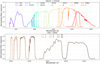 |
Fig. C.1 The combination of filters used and their respective normalized transmission curves. On the top panel, GALEX and S-PLUS filters. In the lower panel, VHS and AllWISE filters. |
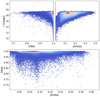 |
Fig. D.1 The relationships between zphot, Odds and r AUTO magnitudes. |
General properties
Photometric properties
All Tables
All Figures
|
Fig. 1 Definition of two categories of spurious objects: those detected close to the spikes of saturated stars and those accumulated at the edges of the images. |
| In the text | |
|
Fig. 2 Confusion matrix for separation of spurious and non-spurious objects for the test sample (20%). On the vertical axis, we show the true source labels, and on the horizontal axis, we show the predicted labels. N represents the number of sources per label. |
| In the text | |
|
Fig. 3 Confusion matrix of PCA model: the one with the highest accuracy and F1 score. N represents the number of sources per label, and the quantities shown correspond to the test sample (20%) of the training sample. |
| In the text | |
|
Fig. 4 From left to right: panels show evolution of the spatial distribution of objects, from the catalog by Haack et al. (2024) (left panel) to the final S+FP extragalactic catalog (right panel); see text for details. |
| In the text | |
|
Fig. 5 Histogram of g band AUTO magnitudes and the choice of photometric depth at 19.5 mag. The distributions correspond to three S/N thresholds (S/N > 3, blue; S/N > 10, red; and S/N > 20, green). |
| In the text | |
|
Fig. 6 Comparison of zspec, provided by SIMBAD and Lima et al. (2022), that were utilized to build the spectroscopic sample employed to validate the zphot estimates. The red line is the identity line. The region colored in gray corresponds to the sources that display Δzspec < 0.03. The galaxies in that region constitute a double-checked sample that includes 85% of the total sources in the plot. |
| In the text | |
|
Fig. 7 Left panel shows comparison between zspec and zphot obtained with a ML approach colored by source density. In the right panel, the comparison is colored by Odds. Below each panel, we also show the corresponding bias. The regions colored in red correspond to the outlier region, according to Eq. (3). The black lines correspond to the identity lines. |
| In the text | |
|
Fig. 8 Top panel presents the evolution of σNMAD with zphot at different zphot bins. Above each bin we show the total number of galaxies considered in the calculation. Error bars and interpolation were calculated with bootstrapping. In the lower panel, we show the variation of σNMAD with rauto. |
| In the text | |
|
Fig. 9 Comparison between true values provided spectroscopically by SDSS DR8 and the values predicted using ML, for stellar mass (left), SFR (center) and D4000N index (right). Each plot is colored according to density, and the black lines correspond to the identity lines. Each lower subplot represents the residual of the respective estimated property. |
| In the text | |
|
Fig. 10 Stellar mass–SFR relation showing the SFMS (left) and stellar mass–sSFR relation (right). Both plots share the same color bar, representing D4000N index values. |
| In the text | |
|
Fig. 11 r − J0660) versus (r − i) color-color diagram for the field ID SPLUS-s29s31 with 10 mag < rband < 16 mag, considering all objects (stars and galaxies). The dashed black line corresponds to the stellar locus fit and the dotted red line represents a 3σ deviation from the stellar locus. We depict four ELGs identified by G25 in cyan and six ELGs by L25 in red. |
| In the text | |
|
Fig. 12 Projected overdensities of the extragalactic catalog (left) superimposed with galaxy clusters identified by eROSITA marked as circles (right). The sizes of the circles are proportional to M500 and the colors correspond to the BEST_Z redshift provided by eRASS1. The central green triangle indicates the position of NGC 1399. |
| In the text | |
|
Fig. A.1 Histogram for the variance explained by each principal component. |
| In the text | |
|
Fig. A.2 star and galaxy separation in a 3D plot constructed with the three main components that contribute most to explaining the variance in the data. |
| In the text | |
|
Fig. A.3 PCA1 and PCA2 feature weights. |
| In the text | |
|
Fig. B.1 Identification and selection of problematic background galaxies. |
| In the text | |
|
Fig. C.1 The combination of filters used and their respective normalized transmission curves. On the top panel, GALEX and S-PLUS filters. In the lower panel, VHS and AllWISE filters. |
| In the text | |
|
Fig. D.1 The relationships between zphot, Odds and r AUTO magnitudes. |
| In the text | |
Current usage metrics show cumulative count of Article Views (full-text article views including HTML views, PDF and ePub downloads, according to the available data) and Abstracts Views on Vision4Press platform.
Data correspond to usage on the plateform after 2015. The current usage metrics is available 48-96 hours after online publication and is updated daily on week days.
Initial download of the metrics may take a while.