| Issue |
A&A
Volume 708, April 2026
|
|
|---|---|---|
| Article Number | A142 | |
| Number of page(s) | 13 | |
| Section | Planets, planetary systems, and small bodies | |
| DOI | https://doi.org/10.1051/0004-6361/202558588 | |
| Published online | 06 April 2026 | |
Thin regolith layer anticipated on the surface of the Tianwen-2 target asteroid (469219) Kamo‘oalewa
1
Research Centre for Deep Space Explorations | Department of Land Surveying and Geo-Informatics, The Hong Kong Polytechnic University,
Hung Hom, Kowloon,
Hong Kong,
China
2
New Material Technology and Marine Engineering Equipment Research Center, The Hong Kong Polytechnic University Wenzhou Technology and Innovation Research Institute,
Wenzhou,
China
3
Department of Civil and Environmental Engineering, The Hong Kong Polytechnic University,
Hung Hom, Kowloon,
Hong Kong,
China
★ Corresponding author: This email address is being protected from spambots. You need JavaScript enabled to view it.
Received:
16
December
2025
Accepted:
18
February
2026
Abstract
Context. Near-Earth asteroid (469219) Kamo‘oalewa is the first target of the ongoing Tianwen-2 sample-return mission. Ground-based observations measured its rotation period at only about 28 minutes, while the low thermal inertia value (Γ = 150 or 181 J m−2 K−1 s−1/2) estimated from the Yarkovsky effect determination implies a thermal insulating layer on the surface.
Aims. The first goal of this paper is to facilitate the sample collection of the Tianwen-2 mission with a prediction of the current status of the possible regolith layer on Kamo‘oalewa. The second goal is to build a framework of regolith evolution on small fast-rotating asteroids as a reference for future observations and studies.
Methods. We used finite element analysis software, Abaqus, to simulate the thermal stress field of Kamo‘oalewa under seasonal and diurnal temperature cycles, with different thicknesses (H) of the regolith layer. At each latitude, the stress excursion at the top of the bedrock as a function of H was incorporated into the ordinary differential equations for regolith total mass and grain size distribution evolutions. The negative feedback between H and thermal fragmentation rate was considered together with regolith removal processes of micro-impact ejecta escape and electrostatic dust lofting in the ordinary differential equations.
Results. The competition between the regolith production and removal processes results in an equilibrium regolith thickness, which increases with latitude due to the seasonal temperature and stress cycles. Under different choices of materials and obliquities and a range of possible fragmentation rates, the equilibrium thickness, H, is estimated to be 0.4–71 mm, equivalent to 0.3–53.5 diurnal regolith thermal skin depth. Our prediction of the equilibrium H satisfies both constraints from thermal inertia observations and cohesive strength estimations on airless bodies.
Key words: planets and satellites: physical evolution / planets and satellites: surfaces / planets and satellites: individual: Kamo‘oalewa
© The Authors 2026
 Open Access article, published by EDP Sciences, under the terms of the Creative Commons Attribution License (https://creativecommons.org/licenses/by/4.0), which permits unrestricted use, distribution, and reproduction in any medium, provided the original work is properly cited.
This article is published in open access under the Subscribe to Open model. This email address is being protected from spambots. You need JavaScript enabled to view it. to support open access publication.
1 Introduction
China’s Tianwen-2 mission (Li et al. 2024a) was successfully launched in May 2025 and is expected to rendezvous with near-Earth asteroid (NEA) (469219) Kamo‘oalewa (de la Fuente Marcos & de la Fuente Marcos 2016) by July 2026. Kamo‘oalewa (provisional designation 2016 HO3) is among the most stable of Earth’s quasi-satellites (Reddy et al. 2017), residing at a distance of ∼100 lunar distances. Light-curve reconstructions indicate that Kamo‘oalewa is a sub-100 m asteroid, with estimated dimensions of 100 m × 81 m × 46 m (Ren et al. 2024b) or 69 m × 58 m × 51 m (Zhang et al. 2024). It rotates with a period of 0.467 ± 0.008 h (Warner et al. 2021), well below the critical period for a gravity-bound aggregate with any reasonable bulk density (Harris 1996; Pravec & Harris 2000). As Kamo‘oalewa is a fast rotator, it requires a monolith or cohesive rubble pile structure in order to not be disrupted by the centrifugal force. Moreover, the short rotation period (τrot) raises a key question: whether a regolith exists, and if so, in what form, on the surface of Kamo‘oalewa. Previous Hayabusa (Yano et al. 2006), Hayabusa-2 (Müller et al. 2017), and OSIRIS-REx (Walsh et al. 2019) missions were all conducted on gravitational-bounded targets. The unknown status of the possible regolith on Kamo‘oalewa poses a challenge for engineering redundancy and also raises intriguing scientific questions about the evolution of small fast-rotating asteroids (SFRAs). Previous numerical modeling works (Ren et al. 2024b; Li & Scheeres 2021) suggest that the van der Waals force is sufficient to retain particles of several millimeters, and the combined effect of thermal fatigue and micro-impacts supports a positive production rate of regolith material (Ren et al. 2024b) for a bare rock situation. However, the regolith production and removal mechanisms for situations in which Kamo‘oalewa is already covered by a regolith layer have not been investigated. From an observational perspective, the surface properties of SFRAs are difficult to constrain from thermal-infrared or other remote observations due to their small sizes. Thermal inertia of two SFRAs were estimated at low values (Fenucci et al. 2021, 2023) based on the comparison between the observed and the modeled Yarkovsky effect (Bottke et al. 2006), which suggested that regolith layers may exist on SFRAs.
Recently Fenucci et al. (2025) estimated the thermal inertia of Kamo‘oalewa at Γ = 150 or 181 J m−2 K−1 s−1/2 from orbit determination and thermal models of the Yarkovsky effect. The corresponding thermal conductivity is in the range of 0.012–0.015 W m−1 K−1, suggesting a regolith layer with an average grain size in the range of ∼0.1–3 mm. Therefore, the existence of a regolith layer on Kamo‘oalewa is not only allowed by the surface dynamical environment (Ren et al. 2024b; Li & Scheeres 2021; Scheeres et al. 2010) but also supported by observational evidence. However, this observational evidence of regolith has not yet been quantitatively linked to the surface dynamical environment and physical processes governing the regolith evolution, such as thermal fatigue and micro-impacts (Ren et al. 2024b).
The aim of this paper is twofold. The first goal is to improve our understanding of Kamo‘oalewa’s regolith structure and to support the upcoming Tianwen-2 sample-collection campaign. The second goal is to provide a framework for regolith evolution on SFRAs that can be tested against future observations. In this paper, we build a numerical model to investigate the evolution of the thickness (H) of the regolith layer on Kamo‘oalewa. We include electrostatic removal of fine-grained regolith (Hsu et al. 2022; Wang et al. 2016; Hood et al. 2018) as a regolith mass-changing process in addition to thermal fatigue and micro-impacts. We divide the structure of Kamo‘oalewa into a thin regolith layer and a monolithic bedrock beneath it, and the evolution of the grain size distribution (Hsu et al. 2022) is coupled with the calculation of regolith thickness. The paper is organized as follows. In Sect. 2, we introduce the context of the possible regolith on Kamo‘oalewa in more detail. In Sects. 3.1 and 3.2, we calculate the diurnal and seasonal temperature and thermal stress fields of Kamo‘oalewa, with different assumptions for H, obliquities, and bedrock materials. In Sect. 4, we present our results on how the regolith production and removal rates change with H and at which H a balance between those processes would be reached. In Sect. 5, we discuss the limitations of our current model and the implications of our results for the possible regolith on Kamo‘oalewa.
2 Context of the possible regolith
2.1 Limit of the regolith layer’s thickness from cohesive strength
In contrast to sub-kilometer or larger asteroids, most of which rotate more slowly than the critical period around 2 h (Hergenrother & Whiteley 2011), Kamo‘oalewa cannot hold large boulders on its surface by gravity. Therefore, the structure of Kamo‘oalewa is likely to be monolithic bedrock covered by multiple layers of regolith grains. The global interface between the regolith layer and the bedrock might be a unique feature of small fast rotators. For this two-layer scenario, as demonstrated in Sánchez & Scheeres (2020), fission failure occurs via stripping of the entire regolith layer at the interface between the bottom grains and the bedrock.
In Sánchez & Scheeres (2020), the rotation speed is gradually increased to test the failure patterns. Here, the rotation period is considered to be constant, while the thickness of the regolith becomes the critical variable in stability analysis. On the other hand, cohesive strength on airless bodies is difficult to directly measure in situ. Previous works suggest a cohesive strength of 75–85 Pa (Hirabayashi & Scheeres 2015) or 64 Pa (Rozitis et al. 2014) for the NEA 1950 DA, 40–210 Pa for the main belt comet P/2013 R3 (Hirabayashi et al. 2014), <25 Pa for 2008 TC3 (Sánchez & Scheeres 2014), and 0.2–20 Pa (Walsh et al. 2022) or <0.001 Pa (Lauretta et al. 2022) for Bennu. For reference, the cohesive strength for weak lunar regolith is measured at 100 Pa (Mitchell et al. 1974). Cohesive strength could also be measured from cratering, and the Small Carry on Impactor (SCI) experiment (Arakawa et al. 2020) conducted by the Hayabusa2 mission provides valuable data. However, depending on whether the impact is interpreted as being in the gravity or strength regime, the cohesive strength is less than 1.3 Pa (Arakawa et al. 2020) or about 20 Pa (Scheeres & Sánchez 2018), respectively.
Given this wide range of possible cohesive strength, we plot three cases with cohesive strengths of σc = 0.2, 1.3, and 10 Pa in Fig. 1 to show the critical thicknesses that trigger fission failure. We adopted a spherical bedrock with a radius of R = 35 m, which has the same volume as the model we reconstructed from light curve data (Ren et al. 2024b). Under the assumption that H ≪ R, the critical thickness was calculated with
 (1)
(1)
where ρ and ϕ are the density and porosity of the regolith material, ω is the angular speed of rotation, g is the gravitational acceleration at the surface, and φ is the latitude. We assumed ρ = 2700 kg/m3 and ϕ = 0.5 for common S-type asteroids, and the corresponding boundaries between fission failure and landslide are at φ = 75.6◦N and 75.6◦S. In each case, H increases about 4 times from the equator to φ = 75.6◦. It is interesting to note that if any processes increase the thickness beyond this upper limit, the centrifugal force will not only remove the exceeded thickness but can strip the entire regolith layer from its bottom (demonstrated in Fig. 3). The σc = 10 Pa case gives a range of upper limit of 16–67 m, which breaks the assumption of H ≪ R. Therefore, the curve for σc = 10 Pa only indicates that σc = 10 Pa is sufficient to retain tens of meters of regolith on Kamo‘oalewa, and does not suggest a real upper limit.
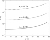 |
Fig. 1 Critical thickness of the regolith layer for the fission-failure region with three different values of the cohesive strength (φ is the latitude). |
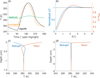 |
Fig. 2 Surface temperature cycle’s responses of different regolith properties. (a) Surface temperature during a rotation period for: only regolith (black), only norite bedrock (green), and bedrock covered by 1ls of regolith (orange). (b) Blue line and left ordinate: Surface temperature excursions divided by the excursion of the regolith-only case (95.2 K) as a function of H/ls. Red line and right ordinate: Normalized κ for different H/ls to obtain the same ∆T as the regolith-only case. (c) Temperature in depth for the regolith-only case. (d) Temperature in depth for a case that norite bedrock is covered with 2ls of standard regolith. |
Different models of bedrock physical parameters and characteristic values of Kamo‘oalewa used to calculate thermal stress fields.
2.2 Synthetic thermal inertia from the regolith-bedrock structure
In addition to the aforementioned upper limit of the regolith thickness, the recent measurement of Kamo‘oalewa’s thermal inertia at  or 181 J m−2 K−1 s−1/2 (Fenucci et al. 2025) also provides clues as to the lower limit of H. While thermal conductivity and particle size are deduced from Γ, the influence of the underlying bedrock with relatively high thermal conductivity is not considered in Fenucci et al. (2025). To demonstrate the possible range of H on the basis of the observed thermal inertia value, we built a 1D planar finite difference model to simulate the diurnal temperature cycle modified from the scheme in Spencer et al. (1989). To explore the basic mechanisms, we simply assumed that any two cases have the same effective thermal inertia (Γeff) if the temperature excursions, ∆T = Tmax − Tmin, of these two cases are the same. We adopted norite properties (density, thermal conductivity, and heat capacity; see Table 1) in simulating the bedrock in this subsection to represent the hypothesis that Kamo‘oalewa was formed from the far side of the Moon (Jiao et al. 2024). More possible origins and types of the material of the asteroid are discussed later in Sect. 3. We used κest = 0.012 W m−1 K−1 (Fenucci et al. 2025) as the standard thermal conductivity of the regolith, and the heat capacity of regolith is c = 800 J kg−1 K−1 (Fenucci et al. 2025). Consequently, the bulk density of the regolith material was calculated by ρ = Γ2/ (κc) = 2344 kg/m3, when the standard value of the regolith thermal inertia is at Γ = 150 J m−2 K−1 s−1/2.
The thermal conductivity of regolith is two orders of magnitude lower than the bedrock’s. This difference significantly changes the amplitude and the penetration depth of temperature cycles, which are characterized by thermal inertia and skin depth,  , respectively. Derived from the norite properties, Γrock = 2536 J m−2 K−1 s−1/2, and bedrock has a skin depth of ls,rock = 1.73 cm. Meanwhile, the skin depth of standard regolith, ls (κest), is only 0.13 cm. For simplicity, we use the symbol ls to refer to ls (κest) = 0.13 cm in the following unless stated otherwise. In Fig. 2a, ∆T drops from 95.2 K to 76.4 K when H is changed from semi-infinite to 1ls. If the bare bedrock is directly exposed to ambient space, ∆T dramatically decreases to 8.4 K. Temperature excursions as a function of H/ls are shown in Fig. 2b. Conversely, to keep ∆T = 95.2 K, the actual κ of the regolith layer needs to be smaller than κest for the two-layer cases. The corresponding values of adjusted κ are shown by the orange line in Fig. 2b. When H/ls = 0.1, i.e., H = 130 µm, the corresponding thermal conductivity is only 7.4 × 10⁻⁴ W m−1 K−1. Such a value is too low for typical NEAs (Delbo et al. 2015; Novaković et al. 2024), and also too low to be a likely property for Kamo‘oalewa (Fenucci et al. 2025). Thus, a lower limit of H at hundreds of µm is imposed by thermal inertia estimations (Fenucci et al. 2025). Nevertheless, the precise value of this lower limit depends on the properties of both regolith and bedrock and the realistic shape of the asteroid.
It seems abnormal that both lines in Fig. 2b are non-monotonic and exceed the reference value when H/ls is roughly between 1.7 and 3.5. Figures 2c and 2d explain this counterintuitive behavior. In these two panels, the orange lines labeled with “Noon” show the temperature profile with depth when the sunlight is perpendicular to the plane, and the blue lines labeled with “Midnight” represent the temperature profile after a half rotation period. In Fig. 2c, phase differences of the temperature cycle exist with depth. At both noon and midnight, local extreme values appear with opposite sign relative to the surface temperature at a depth of ∼2.5ls. This lag of T hinders the further development of the temperature excursion. In Fig. 2d, replacing the regolith below 2ls with high-κ bedrock material is analogous to sticking temperatures at 2ls for the two phases closer together. Thus, the amplitudes of the opposite temperatures at ∼2.5ls significantly decrease, and Tmax and Tmin are able to separate further at the surface. Therefore, for the range of H between 1.7 and 3.5ls, the determined κ for the regolith layer should be higher than κest, and the regolith grains should also be coarser than the estimation for the regolith-only scenario.
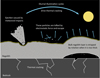 |
Fig. 3 Physical processes that produce and remove regolith on Kamo‘oalewa. The basic scheme of the sketch refers to Fig. 3 in Cambioni et al. (2021). |
3 Models of regolith evolution
In Sects. 2.1 and 2.2, we introduce the upper and lower limit on the thickness of the regolith layer on Kamo‘oalewa, respectively. However, those limits are not enough to predict the current status of the regolith layer without the consideration of transient processes that produce and remove regolith material. Figure 3 shows the mechanisms considered in this work. Because large boulders are not expected on its surface, thermal fragmentation (Delbo et al. 2014; Cambioni et al. 2021; Hsu et al. 2022) of the monolithic bedrock is regarded as the only process that generates regolith (Ren et al. 2024b) on Kamo‘oalewa. Three regolith removal processes are considered: (1) micro-impacts’ ejecta (Ren et al. 2024b); (2) electrostatic dust lofting (Wang et al. 2016; Hood et al. 2018; Hsu et al. 2022); and (3) the peeling of the regolith layer as described in Sect. 2.1. The detailed interactions between these processes will be discussed in the following sections.
In Ren et al. (2024b), we estimated the regolith production rate with the analytical solutions of thermal stress for rotating meteoroids (Čapek & Vokrouhlický 2010). Here, we adopted a more specialized approach that calculates the thermal stress fields of the assumed monolithic bedrock at different obliquity values and seasons. For the purposes of this paper, a spherical shape model is sufficiently representative to investigate the temperature and stress fields of Kamo‘oalewa. Due to the small size and relatively long distance, it is difficult to accurately measure the obliquity (γ) of Kamo‘oalewa from ground-based observations. Adopting data from Zhang et al. (2025) and Ying et al. (2025), γ is derived as 107.8◦ or 135.7◦, respectively. We also obtain an obliquity at 99.3◦ from our reconstructed model (Ren et al. 2024b). Here, we choose 99.3◦ and 45◦ as two typical obliquities to represent two possible of rotation axes: nearly within the ecliptic plane or tilted with a medium angle.
The origin of Kamo‘oalewa is still under hot debate. The spectrum at longer wavelengths and orbital dynamic studies suggest it originated from lunar ejecta (Sharkey et al. 2021; Castro-Cisneros et al. 2023). Moreover, recent studies proposed that the source of Kamo‘oalewa is located at Giordano Bruno crater on the far side (Jiao et al. 2024), or Tycho crater on the near side (Zhu et al. 2025). In contrast, spectral data in the visible and near-infrared wavelengths obtained with the Large Binocular Telescope suggests that Kamo‘oalewa is most likely an S-type asteroid (Reddy et al. 2017; Zhang et al. 2024), which aligns with its spectral properties suggesting a long space weathering exposure and suggesting that it originated in the main asteroid belt, and migrated to the near-Earth region (Zhang et al. 2024; Li et al. 2024b). Orbital simulations also show that the main asteroid belt can serve as a viable source of Kamo‘oalewa-like objects (Wang et al. 2026), and simulation results suggest Kamo‘oalewa is more likely to have originated from the main asteroid belt than the Giordano Bruno crater on the Moon (Fenucci et al. 2026). We do not aim to directly answer the question of the origin of Kamo‘oalewa in this paper. Instead, we consider both hypotheses and investigate the effect of different properties on regolith evolution. We chose ordinary chondrite to represent the S-type and norite for the Giordano Bruno crater origin. In Table 1 we list physical parameters of four models with different obliquities and materials. The regolith material is always assumed to be the standard regolith described in Sect. 2.2. For the temperature and stress fields calculations, we only show results of Model 1 and 2 as examples, and the final results for all models are presented in Sect. 4.
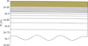 |
Fig. 4 Mesh structure zoomed at the depth of interest. The arc length of the plotted elements corresponds to 1◦. The area with tan color is assigned with regolith materials. |
3.1 Temperature fields
We used the commercial software Abaqus (finite element method) to simulate the temperature and stress fields with diurnal and seasonal sunlight changes. Figure 4 shows the mesh structure. For the top 18 elements, the radial step is 0.5 cm. We set the top 4.5 cm (9 layers of elements) as the regolith layer, and all material below that as the monolithic bedrock. From the 19th cell, biased stepping was adopted, from 1 cm to 1 m. The hexahedral mesh covers a shell covers a shell from R = 32 to 35 m (not all shown in Fig. 4). For the inner spherical region, tetrahedron meshing with biased stepping was adopted to reduce computational expense.
To simulate different regolith thicknesses without changing the mesh, we applied a similarity analysis to the regolith region. The heat conduction is governed by
![Mathematical equation: $\rho c{{\partial T} \over {\partial t}} - \nabla \cdot [\kappa \nabla T] = 0.$](/articles/aa/full_html/2026/04/aa58588-25/aa58588-25-eq4.png) (2)
(2)
The boundary conditions at the top surface of the regolith are
 (3)
(3)
where  is the outward normal vector of a surface element, ε is emissivity, σ is the Stefan–Boltzmann constant, A is bolometric albedo, and FS is the flux of incident sunlight. Similar to the 1D analysis in Spencer et al. (1989), we replaced x with x′ = x/ls. Then Eq. (2) becomes
![Mathematical equation: ${{\partial T} \over {\partial t}} - {\omega ^2}\nabla ' \cdot \left[ {\nabla 'T} \right] = 0,$](/articles/aa/full_html/2026/04/aa58588-25/aa58588-25-eq7.png) (4)
(4)
where ∇′· and ∇′ are the divergent and gradient operators in the dimensionless x′ coordinate, and Eq. (3) becomes
 (5)
(5)
Here we use the subscripts 1 and 2 to denote the realistic and the numerical case, respectively. To have T1 (x′, t) = T2 (x′, t), the properties of the regolith must satisfy H1/ls1 = H2/ls2 and Γ1 = Γ2. At the regolith-bedrock interface, the requirement is also Γ1 = Γ2. There are three free variables, ρ2, c2, and κ2, so we can set c1 = c2 to close the system. As a result, we obtain κ1/κ2 = H1/H2 and ρ1/ρ2 = H2/H1. In this way, we can simulate different thicknesses by changing only the input density and thermal conductivity values of the regolith material. This also means that the physical properties of the regolith material can be decoupled from those of the bedrock material, as long as the targeted Γ and ls are matched.
3.1.1 Seasonal temperature fields
Subsurface temperatures vary with orbital position if the obliquity is not 0 or 180◦ and the eccentricity is not 0. For simplicity, we neglected the effect of the orbital eccentricity and assumed that e = 0. The orbital phase, θ, is defined as the angular distance past the configuration in which the south pole points toward the Sun. The energy influx from the incident sunlight vector is averaged over one rotation period. Therefore, the seasonal temperature evolution is essentially a 2D problem, but we still simulated it in a 3D model to better connect with the subsequent diurnal temperature and stress models.
We adopted one year as the orbital period for Kamo‘oalewa. The corresponding seasonal skin depth for bulk norite is 2.60 m, which is about 140 times of the diurnal rock skin depth, ls,rock = 1.89. Figure 5 shows the seasonal temperature cycles for the surface element of the bedrock when it is covered with a regolith layer of H = 2ls. The pattern of the temperature cycles transitions gradually from a double-peaked to a single-peaked form from the equator to the north pole. The southern hemisphere experiences the same temperature history, phase-shifted by half an orbital period. The seasonal temperature excursion, ∆TS, increases with φ. This trend is shown for different thicknesses of the regolith layer from 0 to 100ls in Fig. 6 for both models. The temperature excursions at low latitudes are 2–3 times larger when γ = 99.3◦ than when γ = 45◦, but generally become closer at high latitudes. Low-κ regolith acts as an efficient insulator: a layer of 10ls (only 1.3 cm thick) can reduce the seasonal temperature variation by about half relative to the bare-bedrock case. From another aspect, because the orbital period is 18 770 times the rotation period, the decay of ∆TS with H is much slower than that of the diurnal temperature excursion, as is discussed below.
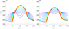 |
Fig. 5 Seasonal temperature cycles for the top of the bedrock for H = 2ls. Latitudes from the equator to the north pole are represented by lines with colors from blue to red (θ is the orbital phase). Panels a and b show the cases for Model 1 and Model 2, respectively. |
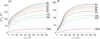 |
Fig. 6 Seasonal temperature excursions of the top of the bedrock at different latitudes. Panels a and b show the cases for Model 1 and Model 2, respectively. |
3.1.2 Diurnal temperature fields
In Sect. 2.2, we focus on the influence of the bedrock on the surface temperature of the regolith, and in this section our interest is the reverse: how the existence of the regolith layer affects the temperature field of the near-surface bedrock. Different bedrock materials, obliquity, orbital phase, regolith thickness, and latitude jointly determine the diurnal temperature field. We adopted parameters γ = 99.3◦, θ = 270◦, and H/ls = 2 as an example. Figure 7a shows continuous temperature profiles of the near subsurface over one rotation cycle with different scaled axes for the regolith and bedrock regions. Figure 7b shows the temperature of the surface of the bedrock at different times within one rotation period and at different latitudes. The variations along latitudes are inherited from the seasonal temperature cycle, and the variations regarded to time are due to the diurnal rotation. It is also interesting to notice that T is high around midnight at the surface of the bedrock because the regolith layer with a thickness of 2ls results in a phase difference of about half a period.
Next, we move to more general situations where the diurnal temperature excursion (∆TD) is a function of γ, θ, and H/ls.
In Fig. 8, ∆TD (φ) is shown for γ = 99.3◦ in panel a and for γ = 45◦ in panel b. The most important feature is that ∆TD decays rapidly with the increase in H. Among the two selected obliquities, values of ∆TD (φ) are almost the same at equinox, which is consistent with the similar rotation statuses. However, at θ = 0, ∆TD decreased significantly in Model 1. The northern hemisphere is always opposite to the sunlight during that orbital phase, so ∆TD is essentially 0 for all H. For the cases with γ = 45◦, ∆TD is still considerable at θ = 0, especially for the southern hemisphere, which is experiencing “summer”. Finally, it is apparent that if γ = 0 or 180◦, ∆TD (φ) will remain the same at any orbital position.
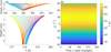 |
Fig. 7 Diurnal temperature field example at γ = 99.3◦, θ = 270◦, and H/ls = 2. (a) Temperature at depth at φ = 0 for regolith (upper) and near-surface bedrock (bottom). Lines with different colors represent different times, beginning with dark blue at midnight. (b) Temperature contour in the space of latitude and time within one rotation period. |
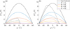 |
Fig. 8 Diurnal temperature excursions. The left half of the abscissas is for the southern hemisphere and the right half for the northern. The solid lines represent cases at equinox (θ = 270◦), and the dashed lines represent cases when θ = 0. Cases with different H are plotted from 0 to 5ls with different colors. Panels a and b show the cases for Model 1 and Model 2, respectively. |
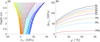 |
Fig. 9 Seasonal stress field for Model 1. (a) Seasonal thermal stress profiles at φ = 0◦ and H = 2ls. Orbital phases begin at θ = 0 with the dark blue line and end at θ = 180◦ with the dark red line. (b) Seasonal thermal stress excursions with different thicknesses of the regolith layer. |
3.2 Thermal stress fields
After the temperature fields of interest were calculated, we continued to use Abaqus and adopted a sequentially coupled thermal-stress analysis, in which the temperature fields were applied as predefined fields. In this step of our model, the regolith layer is considered as loose material that does not provide mechanical constraints, and thus we assigned a symbolic low Young’s modulus of 5 Pa to the regolith material to maintain stability. This gave us a convenient way to transfer temperature results to the stress simulation with the same mesh. The term “depth” used in this section refers to the normal distance below the surface of the bedrock, not below the actual asteroid’s surface. In reality, the plane of crack growth might change with time and be complicated with respect to the diurnal and seasonal effects. Here, for simplicity, we built a right-hand coordinate, where Y is the rotation axis, and chose elements at x = 0 as the investigated objects. According to Paris law (Paris et al. 1963; Delbo et al. 2014), σzz would be the component that contributes to the growth of cracks for the selected region. The governing equations used to calculate the thermal stress tensor, σ, can be found in Čapek & Vokrouhlický (2010).
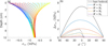 |
Fig. 10 Diurnal stress field for Model 1. (a) Diurnal thermal stress profiles at φ = 0. The colors of the lines represent different times through one rotation period. (b) Diurnal thermal stress excursions with different thicknesses of the regolith layer. Solid lines show the cases when θ = 270◦, and dashed lines show the cases when θ = 0. |
3.2.1 Seasonal stress fields
Figure 9a shows the seasonal change in σzz with depth, with the example of Model 1 and φ = 0◦. Only half an orbit is plotted because, similar to the double-peak pattern in Fig. 5, the stress field exhibits a double-peaked pattern. For materials near the equator, the stress field history can be considered symmetric when θ changes from 0 to 180◦ and from 180 to 360◦; thus, these locations effectively experience two temperature and stress cycles per orbital period. Figure 9b shows the seasonal stress excursion, ∆σzz (φ), for different H/ls at γ = 99.3◦. Compared with Fig. 6a, ∆σzz is approximately proportional to ∆TS (K), with ∆σzz/∆TS ≈ 0.7 MPa K−1.
3.2.2 Diurnal stress fields
As ∆TD is much smaller than ∆TS, the diurnal stress excursion is also much smaller than the seasonal stress excursion. The thermal stress shown in Fig. 10a extends to a depth of ∼6ls (rock), and already converges closely at 10 cm. Due to different temperature cycles and thus different skin depths, the diurnal thermal stress penetrates much less deeply than the seasonal one, as is shown by Figs. 9a and 10b. The diurnal ∆σzz (φ) curves in Fig. 10b are also very similar to the ∆TD (φ) curves in Fig. 8a, while the amplitudes are one to two order of magnitudes lower than the seasonal stress excursions.
3.3 Thermal fragmentation
In Sect. 3.2, we introduced the seasonal and diurnal thermal stress variations in the monolithic bedrock of Kamo‘oalewa. In previous studies on airless bodies, the fragmentation rates are derived from the time required to break through particles and/or boulders by a sole crack plane (Delbo et al. 2014; Mir et al. 2019; Cambioni et al. 2021). A similar strategy was also adopted in our previous work (Ren et al. 2024b). Here, we additionally estimated the thermal fragmentation rate (Rbf) for the large-scale intact bedrock part of the asteroid. The fatigue crack growth law, Paris law (Janssen et al. 2004; Delbo et al. 2014), relates the crack growth rate to the maximum stress intensity factor excursion, ∆KI:
![Mathematical equation: ${{{\rm{d}}a} \over {{\rm{d}}N}} = C{\left[ {{\rm{\Delta }}{K_I}(a)} \right]^n},$](/articles/aa/full_html/2026/04/aa58588-25/aa58588-25-eq9.png) (6)
(6)
where a is the crack length, N is the number of cycles, and C and n are material properties. We adopted n = 3.84 and ![Mathematical equation: $C = 3 \times {10^{ - 4}}{\rm{m }}{[{\rm{MPa}}\sqrt {\rm{m}} ]^{ - n}}$](/articles/aa/full_html/2026/04/aa58588-25/aa58588-25-eq10.png) for Carrara marble (Migliazza et al. 2011), consistent with calculations for asteroid and meteorite materials in Delbo et al. (2014). The expression of KI can be obtained with the corresponding geometry by Glinka & Shen (1991). If we apply the crack growth calculation (Delbo et al. 2014) to Model 1 with H = 0, for example, we obtain a growth rate of 9 cm/yr at the equator, corresponding to a cracked mass production rate of 8.5 × 10⁻⁶ kg m−2 s−1. This rate is apparently overestimated because interactions of multiple crack planes are required to generate fragments in the bedrock. In the previous studies (Delbo et al. 2014; Mir et al. 2019; Cambioni et al. 2021), an initial crack (e.g., 30 µm) is always assumed in each particle. However, for the entire surface of the asteroid, the crack initiation should happen with probability density (m−2 s−1) that is related to the external environment, such as impact influx. On the other hand, cracks can continue growing in the bedrock after they cut off some fragments, and thus external initiations of cracks are not always necessary.
for Carrara marble (Migliazza et al. 2011), consistent with calculations for asteroid and meteorite materials in Delbo et al. (2014). The expression of KI can be obtained with the corresponding geometry by Glinka & Shen (1991). If we apply the crack growth calculation (Delbo et al. 2014) to Model 1 with H = 0, for example, we obtain a growth rate of 9 cm/yr at the equator, corresponding to a cracked mass production rate of 8.5 × 10⁻⁶ kg m−2 s−1. This rate is apparently overestimated because interactions of multiple crack planes are required to generate fragments in the bedrock. In the previous studies (Delbo et al. 2014; Mir et al. 2019; Cambioni et al. 2021), an initial crack (e.g., 30 µm) is always assumed in each particle. However, for the entire surface of the asteroid, the crack initiation should happen with probability density (m−2 s−1) that is related to the external environment, such as impact influx. On the other hand, cracks can continue growing in the bedrock after they cut off some fragments, and thus external initiations of cracks are not always necessary.
In addition, the crack growth rate determination with Eq. (6) tends to overestimate the crack growth rate for airless bodies because of the following reasons. (1) As is pointed out in Molaro et al. (2017), the crack initiation stage is not described in Paris law but can account for the majority time (>70%) of an object’s total lifetime (Janssen et al. 2004). This limitation is less important in a continuous-cracking scenario, in which preexisting cracks are abundant. (2) Paris law is derived from experiments with controlled fatigue loads. However, in the context of thermal fatigue on airless bodies, the thermal stress field is partially released as the crack growth (as shown in Mir et al. 2019), introducing strong nonlinearity. (3) Mechanisms such as crack closure and opening can also affect the form of KI (Paris et al. 1999).
Considering the complexity of fragmentation mechanisms on airless bodies and the limits of direct application of Paris law, we did not compute fragmentation rates directly from crack-growth calculations. Instead, we adopted a nominal value of the bedrock thermal fragmentation rate of r0 = 5 × 10⁻¹¹ kg m−2 s−1 (Hsu et al. 2022), which is 100 times lower than the terrestrial value and also within the range of < 10−10 kg m−2 s−1 inferred from the Hayabusa2 SCI experiment (Sugita et al. 2019; Arakawa et al. 2020). The bedrock fragmentation rate under different conditions was then written as
 (7)
(7)
where F (φ, H) is a fragmentation intensity factor as an auxiliary function and F0 is a reference value that reproduces the nominal rate, r0. Both rfrag,b and F also depend on the chosen obliquity and material model, but we omit this dependence here for brevity. We assumed that the fragmentation rate is proportional to the crack growth rate. Although Eq. (6) does not precisely describe all physical processes that happen in the bedrock, it captures the qualitative trend that larger KI and higher fatigue frequency yield higher fragmentation rates. By dimensional analysis (Molaro et al. 2017), KI is proportional to ∆σ for a given geometry. Therefore, we define
![Mathematical equation: $F(\varphi ,H) = {\left[ {{\rm{\Delta }}{\sigma _{\rm{S}}}(\varphi ,H)} \right]^n}/{\tau _{{\rm{orb}}}} + {1 \over 4}\mathop \sum \limits_{i = 1}^4 {\left[ {{\rm{\Delta }}{\sigma _{\rm{D}}}\left( {\varphi ,H,{\theta _i}} \right)} \right]^n}/{\tau _{{\rm{rot}}}},$](/articles/aa/full_html/2026/04/aa58588-25/aa58588-25-eq12.png) (8)
(8)
where ∆σD and ∆σS are the diurnal and seasonal stress excursions at the top of the bedrock, and τorb is the orbital period. The seasonal variation in ∆σD was accounted for by averaging over four orbital positions, θi ∈ {0◦, 90◦, 180◦, 270◦}. We used an inverse polynomial fit to interpolate ∆σD (φ, H) and ∆σS (φ, H) to arbitrary H from the discrete results in Sect. 3.2. The fit functions were written in a form of  , for the diurnal stress excursions and
  for the seasonal stress excursions, where the fit coefficients pn were determined in a least-squares sense. The fragmentation intensity factor was averaged over one orbital period (1 yr) because variations within the time of 1 yr are not important compared to the long timescale of regolith evolution.
The next step was to determine the value of F0, i.e., to specify the latitude and regolith thickness at which the fragmentation rate matches the nominal value. We first set the thickness at H = 2ls. The thickness of 2ls can be considered as a minimum value to ensure that the bedrock does not act as a heat sink that biases the surface thermal inertia measurement (see Sect. 2.2). (see Sect. 2.2). We then defined lower and upper bounds for F0 as
 (9)
(9)
 (10)
(10)
where Nφ is the number of data points included in the calculation. Because the seasonal contribution of F is stronger than the diurnal contribution, F increases monotonically with φ within a certain hemisphere, and thus F0,α < F0,β. Averaging F0,α and F0,β over all four models yields ![Mathematical equation: $\overline {{F_{0,\alpha }}} = 0.074{\rm{ }}{[{\rm{MPa}}]^{\rm{n}}}{{\rm{s}}^{ - 1}}$](/articles/aa/full_html/2026/04/aa58588-25/aa58588-25-eq17.png) and
and ![Mathematical equation: $\overline {{F_{0,\beta }}} = 1.6{\rm{ }}{[{\rm{MPa}}]^{\rm{n}}}{{\rm{s}}^{ - 1}}$](/articles/aa/full_html/2026/04/aa58588-25/aa58588-25-eq18.png) . Substituting
. Substituting  and
and  into Eq. (7), we defined the lower bound of the thermal fragmentation rate at a given φ and H as
  , and the upper bound as
  , spanning a range of approximately a factor of 20.
To investigate the interactions of different processes, it is necessary to assign the mass production rate to each grain size population. The regolith production rate from the bedrock for the ith population was calculated as
 (11)
(11)
where α (mi) is the mass fraction of the ith grain population produced from fragmentation of the bedrock. The distribution of fragments follows a power-law mass distribution, pf (mi) ∝ m−1.7 (Langevin & Arnold 1977; Hsu et al. 2022). The corresponding expression for α (mi) is then
 (12)
(12)
where imax is the index of the population with the largest grain radius, and ∆mi is the mass bin width of the ith population.
The fragmentation rate of the regolith layer was calculated on the basis of the bedrock fragmentation rate. Taking into account that the regolith layer experiences a higher temperature excursion than the bedrock, we defined a primary regolith fragmentation rate as
 (13)
(13)
For the ith grain population, the fragmentation loss rate was written as
 (14)
(14)
where ai is the radius, fvolume (mi) is the total volume fraction of the ith grain population, and wf (ai, ls) is a scale-adjustment factor. We used the volume fraction rather than the area fraction (Hsu et al. 2022) to more realistically represent fragmentation occurring throughout the entire regolith layer. Scaling arguments (Mir et al. 2019; Cambioni et al. 2021) indicate that particles smaller than the regolith skin depth experience weak temperature gradients, and therefore require longer to break up than particles with diameters of ∼ls. Accordingly, we computed wf (ai, ls) = (2ai/ls)n−1 (Mir et al. 2019; Cambioni et al. 2021). We adopted a similar scheme as in Hsu et al. (2022) to relate the production rate from regolith fragmentation for the ith population, Sfrag,r, to the loss rate with
 (15)
(15)
where β(mi, mj) is the mass fraction of the ith grain population produced from fragmentation of the jth (larger-grain) population, given by
 (16)
(16)
3.4 Micro-impacts
Micro-impacts are considered a process that removes regolith to space and a mechanism that can initiate cracks in both bedrock and regolith grain. Our previous study (Ren et al. 2024b) shows that all micro-impact ejecta escape because even the minimum ejecta velocity exceeds Kamo‘oalewa’s low escape velocity (∼0.04 m s−1). For unconsolidated target material, the mass loss rate caused by micro-impacts ranging between 1.46 and 2.92 × 10⁻¹² kg m−2 s−1 (Ren et al. 2024b) for impactors of 100– 200 µm (Nesvorný et al. 2010). Here, we increase the total mass loss rate to rimp = 1 × 10⁻¹¹ kg m−2 s−1 to represent material launched by the outgoing shock (Housen & Holsapple 2011). Under the dynamical environment of SFRAs, even ejecta with very low vertical launch speeds are likely to escape due to the rotation speed, because van der Waals forces decay rapidly with increasing particle separation (Scheeres et al. 2010). The micro-impact mass-removal rate for the ith grain population is written as
 (17)
(17)
Since all ejecta escape into space, there is no regolith production term from impacts. Applying the point source scaling model (Housen & Holsapple 2011) in the strength regime, the corresponding crater depths are 0.47 and 0.92 mm for impactors with D = 100 µm and D = 200 µm, respectively. This implies that for H ≲ 0.5 mm, micro-impacts can penetrate the regolith layer and strike the bedrock. Thus, the probability of crack initiation should increase as H decreases. The contribution of micro-impacts to the bedrock’s crack growth as a function of H is not captured by the trend of rfrag (H). The actual relationship between crack initiation and H is not specifically modeled here, but it would be interesting to explore in the future.
3.5 Electrostatic dust lofting
Phenomena such as dusk horizon glow (Criswell 1973; Rennilson & Criswell 1974) observed on the lunar surface and fine dust deposits in craters on Asteroid 433 Eros (Robinson et al. 2001), along with many other observations (Wang et al. 2016), have been suggested to be related to electrostatic dust lofting and transport. Laboratory experiment shows that, under simulated NEA conditions, electrostatically lofted dust particles include both individual particles and aggregates, spanning a size range from 7 µm (limited by the image resolution) to 140 µm (Wang et al. 2016). Laboratory experiments also indicate that dust lofting begins at a relatively high rate (5 × 10⁴ particles m−2 s−1) on an initialized surface and slows down as time progresses (Hood et al. 2018). Filling of microcavities and the removal of loose upper layers have been suggested as possible causes of this slowdown (Hood et al. 2018). It would be interesting to test, in situ or in the laboratory, how electrostatic dust lofting evolves under a short rotation (irradiation) period of <1 h, such as Kamo‘oalewa’s τror = 0.467 h. Here we adopted a milder dust lofting rate of rloft = 200 particles m−2 s−1, considering the long timescale of regolith evolution (Hsu et al. 2022). The loss rate due to dust lofting is written as
 (18)
(18)
where farea (mi) is the area fraction of the ith grain population, and memax is the mass of the largest particle that can be lofted by electrostatic force, assumed here to correspond to a particle diameter of 100 µm.
Unlike asteroids with radii of over hundreds of meters and rotation periods of 5 h investigated in Hsu et al. (2022), Kamo‘oalewa’s surface linear rotation speed exceeds its escape velocity at most latitudes. For example, in our spherical model, lofted particles with any launch speed will escape from regions where φ < 72◦. Near the poles, the probability that lofted particles fall back to the asteroid depends on the launch velocity, and those returning particles could land anywhere on the surface. We simplified the model by assuming that all electrostatically lofted particles escape from the asteroid, given that the relevant high latitude areas account for only <5% of the total surface area.
3.6 Integrated regolith evolution model
We integrated three processes – thermal fragmentation, micro-impact ejection, and electrostatic dust lofting – to model the regolith mass (thickness) evolution, together with the grain size distribution. The total mass of regolith was sorted into imax radius bins on a logarithmic scale. We assumed that both regolith grains and fragments produced by bedrock thermal fragmentation span diameters from 1 µm to 1 mm. Substituting a = 0.5 µm into the scale-adjustment factor wf, we obtain wf = (1 µm/ls)n−1 = 1.4 × 10⁻⁹. This indicates that, compared to a reference grain with a diameter of ls = 1.3 mm, fragmentation of the smallest grains is negligible. On the other hand, particles larger than 1 mm may not be able to be retained on Kamo‘oalewa because the relative strength of van der Waals forces compared with centrifugal forces decreases with grain size (Ren et al. 2024b; Li & Scheeres 2021; Scheeres et al. 2010). Larger boulders with sizes of decimeters to meters would not be possible to retain on their surface unless mechanically trapped. Crack production of grains >1 mm, and any subsequent loss processes, would be an interesting topic but is beyond the scope of this paper. For all regolith grain populations, mass evolution was solved using a series of ordinary differential equations (Hsu et al. 2022):
 (19)
(19)
where Mi is the total mass of the ith grain population per unit area, and t is time. The specific forms of the terms on the right-hand side are introduced in the subsections above. Summing over all grain populations, the regolith thickness is
 (20)
(20)
where ρr and ϕ are the density and porosity of the regolith layer. As an initial condition, we set H(0) = 2ls and adopted a power-law size distribution with a differential index of –3.5 (Hsu et al. 2022), comparable to indices derived for disrupted asteroids (Jewitt et al. 2010; Moreno et al. 2016).
It is important to note that, to derive Eqs. (19) and (20), we assumed that the regolith layer is well mixed at all times. In a more realistic setting, the grain size distribution should depend on depth, because micro-impacts, regolith thermal fragmentation, and electrostatic lofting are more intense near the surface, whereas bedrock fragmentation produces grains at the bottom of the regolith layer. One consequence of this assumption is that electrostatic lofting is likely to be overestimated during the early stage but underestimated during the late stage. The validity of this assumption and its other implications are discussed in Sect. 5.
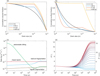 |
Fig. 11 Regolith grain size and thickness evolution for Model 1. (a) Cumulative volume fraction at the equator. (b) Cumulative surface fraction at the equator. (c) Evolution of mass changing rates at the equator. We show the transient processes of bedrock thermal fragmentation (blue line), micro-impacts ejecta (red line), electrostatic dust lofting (green line), and regolith thermal fragmentation (brown line). (d) Thickness evolution at different latitudes. The colors for latitudes change from blue at the equator to red at the pole. The left and right ordinates show dimensionless and dimensional thicknesses of the regolith layer, respectively. |
4 Results
We simulated regolith grain size and thickness evolution for the four models (see Table 1). In Fig. 11 we show the Model 1 case with rfrag,b (φ, H) = rfrag,min (φ, H) as an example. During the first several hundred years, electrostatic dust lofting is the most intense process and reduces the total regolith mass at all latitudes. This occurs because fine grains, which are most susceptible to electrostatic lofting, are abundant at this stage. However, electrostatic dust lofting becomes less important after the fine grains are depleted, and the final balanced state is largely determined by the negative feedback between the regolith production of bedrock thermal fragmentation and H. At the equator, the balanced state is reached after ∼0.1 Myr, with a final thickness of 0.43ls.
Estimated from the constant impact ejection rate alone, the removal rate is 13.5 cm Myr−1, equivalent to about 10 kyr per regolith skin depth. Compared with the timescale of regolith evolution, this refreshing rate indicates that the initial grain size distribution has only a minor influence on the final grain size distribution and the equilibrium thickness. On the other hand, the grain size distribution of thermal-cracking fragments affects regolith evolution continuously. Our result shows that the depletion process of fine grains (≤100 µm) on Kamo‘oalewa is completed within 0.1–1 Myr after initialization. As is noted in Hsu et al. (2022), the abrupt grain mass cutoff (memax) assumed in the electrostatic removal calculation is not realistic, so distributions with smoother turning points are expected in panels a and b. In Fig. 11d, the equilibrium thickness increases from the equator to the pole, from 0.43ls (0.56 mm) to 12.3ls 16.0 mm), because seasonal bedrock thermal fragmentation is more efficient at higher latitudes. Meanwhile, the centrifugal acceleration acen = ω2R cos φ decreases fast with the increase in latitude φ at high latitudes. Therefore, the mild increase in H in high-latitude regions alone is unlikely to trigger the landslide failure (Sánchez & Scheeres 2020) ahead of the fission failure at relatively low latitude regions. On the other hand, it has been suggested that global vibrations, such as impact-induced seismic shaking (Richardson et al. 2004; Thomas & Robinson 2005), cause regolith migration on Itokawa (Miyamoto et al. 2007), but the effects of these vibrations on SFRAs are still unclear.
The equilibrium regolith thickness was determined by the relative rates of the competing processes. To explore the plausible range of H, we varied only the thermal fragmentation rates and kept the rates of the other processes fixed. We show the equilibrium regolith thickness as a function of latitude in Fig. 12. The lower bounds correspond to rfrag,b (φ, H) = rfrag,min (φ, H), and the upper bounds correspond to rfrag,b (φ, H) = rfrag,max (φ, H). When both seasonal and diurnal thermal fragmentation processes are included, H increases from the equator to the poles for all models. The seasonal fragmentation rate increases with φ, whereas the diurnal fragmentation rate decreases with φ, as is shown in Figs. 9b and 10b, respectively. Our results therefore imply that seasonal thermal fatigue contributes more important than diurnal thermal fatigue to regolith production on Kamo‘oalewa. However, the 1-yr period of the seasonal fatigue cycle deviates substantially from the short fatigue periods used in laboratory experiments and in engineering-based fatigue crack-growth theories (e.g., Janssen et al. 2004; Paris et al. 1963). Whether Eq. (6) is appropriate for quantifying the relative intensities of diurnal and seasonal fragmentation therefore remains an open question. We thus also show an end-member case including only diurnal fragmentation (dashed lines in Fig. 12), which also corresponds to scenarios in which γ is very close to 0 or 180◦. In these diurnal-only cases, H decreases mildly away from the equator and then drops steeply beyond ∼75◦.
The reference fragmentation intensity factor,  , for the diurnal-only cases was calculated as the mean value of the diurnal component of F over latitude and is 0.004 [MPa]n s−1. F0,D is 19 times lower than
  , so we have already increased the thermal fragmentation intensity in these diurnal-only cases. Even so, the dashed lines in Fig. 12 are general lower than the shaded regions. Comparing Figs. 9b and 10b, we see that the seasonal stress excursion is less sensitive to changes in H, because the seasonal temperature excursion retains a substantial fraction of its amplitude after penetrating a regolith layer of a few diurnal skin depths. If seasonal fragmentation is less efficient than the diurnal one, a regolith-thickness distribution similar to the dashed lines may be observed by the Tianwen-2 mission. Conversely, if a thicker regolith is observed at higher latitudes, seasonal thermal fatigue would be a plausible explanation in addition to the smaller centrifugal force at high latitudes.
Comparing the results of different models, near the equator the predicted H is larger in the models with γ = 99.3◦ than in the models with γ = 45◦. Apart from this difference, the choice of different obliquity does not change H (φ) significantly. However, as was discussed above, changing the obliquity to values close to 0 or 180◦ will produce a H (φ) curve with a shape similar to the dashed lines but a smaller amplitude. When the asteroid consists of OC, a slightly thicker regolith layer is expected than in norite scenarios. The effect of the micro stress field induced by inclusions (Delbo et al. 2014) is not considered in this paper. In general, the presence of inclusions accelerates the crack growth (Ren et al. 2024b; Delbo et al. 2014). Molaro et al. (2025) simulated that stresses are radial to inclusions during cooling and circumferential to inclusions during heating, and that cracks form perpendicular to the stress orientation. The form and distribution of inclusions in different types of rocks may therefore play an important role in thermal fragmentation.
The equilibrium H of all models is less than 7.2 cm, while the upper limit of H given by a cohesive strength of σc = 0.2 Pa is larger than 30 cm at all latitudes (see Fig. 1). The black line in Fig. 12a shows that H (φ) from the thickest scenario is supported by a cohesive strength at only 0.055 Pa, and the fission failure is most likely to be triggered around φ = 35◦. Therefore, the thickness of the regolith layer on Kamo‘oalewa is not likely constrained by the value of cohesive strength but by the balance between micro-impact ejecta, thermal fragmentation, and electrostatic dust lofting, on the basis of our assumptions of the thermal fragmentation rates. It is possible for the peeling-off process of segments of the regolith layer, shown in Fig. 3, to happen if the balanced H is systematically underestimated in our result by a factor of >10. On the other hand, the lower limit of H constrained by the thermal inertia observations is also satisfied at most latitudes. This feature is a reasonable outcome of the model, since we link the nominal fragmentation rate with the thickness of 2ls. To summarize, we suggest that Kamo‘oalewa is covered by a thin regolith layer of up to several centimeters, and the polar areas are likely to retain a thicker regolith due to seasonal thermal fragmentation and a more stable dynamic environment (Ren et al. 2024b).
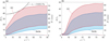 |
Fig. 12 Equilibrium regolith thicknesses at different latitudes. Panels a and b show the results for models with γ = 99.3◦ and γ = 45◦, respectively. The equilibrium thickness ranges for ordinary chondrite material are shown by the shaded red areas, and the ones for norite material by the blue. The dashed lines represent scenarios with only diurnal thermal fragmentation, with the same choice of colors for the different materials. The left and right ordinates show dimensionless and dimensional thicknesses of the regolith layer, respectively. In panel a, the black line indicates that the highest H (φ) is allowed by a cohesive strength of 0.055 Pa. |
5 Discussions
5.1 Thermal stress fields and fragmentation rates
Kamo‘oalewa is widely considered a monolithic asteroid due to its short rotation period, and our thermal stress model is built on this premise. However, the probability of it containing a rubble-pile-like structure has not been directly ruled out. Meteorite evidence and thermal models suggest that fragmentation and reassembly events of ordinary chondrite parent bodies were prevalent in the early Solar System (Lucas et al. 2020; Ren et al. 2024a). The two end-members of a small asteroid’s internal structure can be viewed as a single elastic boulder and a rubble pile aggregated together only by self-gravity. The latter apparently cannot hold Kamo‘oalewa together against the centrifugal forces. The thermal stress field of a intermediate case with inherent cohesion is therefore an intriguing problem. For bare-bedrock cases, the maximum displacement amplitudes induced by seasonal temperature cycles are 1.36 cm for Model 1 and 1.55 cm for Model 3. In addition to the centrifugal forces, the internal cohesion must also be strong enough to counter periodic displacement mismatch driven by temperature cycles. Once this criterion is met, the magnitude of stress excursions in such an intermediate case should be smaller than the monolithic case, because the size of the elastic rock decreases from the whole asteroid to individual blocks. Smaller stress excursions lead to a lower thermal fragmentation rate. The effects of internal structure on regolith evolution are therefore an interesting but complex problem.
In Sect. 3.3, we used only ratios of stress excursions to determine the corresponding fragmentation rates for different scenarios. Here, we compare the absolute values of Kamo‘oalewa’s thermal stress fields with other studies. As is shown in Mir et al. (2019), a 40 cm diameter spherical carbonaceous chondrite without any preexisting cracks, at 1 AU and with a 6 h diurnal cycle, has a stress excursion of 4 MPa. Their numerical results imply a corresponding lifetime of ∼20 Myr. Our equatorial diurnal stress excursions are of the same order of magnitude as those in Mir et al. (2019), even though ∆TD in our model is smaller due to a shorter rotation period and the presence of an additional regolith layer. This outcome is largely attributable to the much larger size of our simulated object. Molaro et al. (2017) computed that boulders on the lunar surface experience stress excursions from ∼2 to ∼30 MPa as diameters increase from 0.3– 50 m. They suggest that a minimum strength of ∼2.4 MPa is required to initiate fatigue breakdown, if only thermal cracking is considered to interpret the steep increase in ≤30 cm boulders found at the Chang’ E-3 landing site (Di et al. 2016). As a tidally locked body, the Moon’s rotation and orbital periods are identical. The lunar thermal stress cycle of ∼27 days lies between Kamo‘oalewa’s diurnal and seasonal cycles, and the stress excursions for a 50 m lunar boulder also fall between Kamo‘oalewa’s diurnal and seasonal stress excursions. Considering the absolute values of diurnal and seasonal stress excursions at H = 2ls and Kamo‘oalewa’s rotation period, it is consistent with previous studies on airless bodies (Delbo et al. 2014; Molaro et al. 2017; Mir et al. 2019; Hsu et al. 2022) to relate a nominal fragmentation rate of 5 × 10⁻¹¹ kg m−2 s−1 with this thickness of regolith. Therefore, our regolith evolution model not only provides a dynamic explanation for the observed low value of thermal inertia (Fenucci et al. 2025), but also independently predicts that a regolith layer exists on the surface of Kamo‘oalewa.
5.2 Impacts with different scales
As is shown in Fig. 11a and b, the regolith layer mostly consists of grains >100 µm, because electrostatic lofting efficiently removes finer grains. Meanwhile, the typical size of influx micro meteoroids ranges from 100 to 200 µm (Nesvorný et al. 2010). Therefore, the micro-impacts on Kamo‘oalewa likely occur in a regime in which the projectile is comparable to, or smaller than, the typical grain of target material. As has been noted in studies (Housen & Holsapple 2011; Cintala et al. 1999, e.g.,), grain size can significant affect energy and momentum coupling, and thus the resulting ejecta mass. Cintala et al. (1999) conducted impact experiments on coarse sand targets (Cintala et al. 1999) and found that scaling law exponents determined from scaled crater dimensions and ejection-speed distributions are substantially different. For Kamo‘oalewa, grain-size effects on ejecta mass, crater depth, and shock wave propagation are therefore important. These effects are not included in this paper but should be investigated in future work.
Considering the dynamic environment of Kamo‘oalewa’s surface, a large-scale impact could reset the surface (Ren et al. 2024b). Li et al. (2024b) estimate that an impact on Kamo‘oalewa with a projectile larger than 0.5 m occurs per 2.063 × 10⁸ yr. This timescale is more than 200 times longer than the evolution times required to reach a balanced state in all our models. In our model, recovery of the balanced regolith state after any refresh events can be considered to be relatively swift (0.1–1 Myr) compared with the frequency of large-scale impacts.
5.3 Assumptions and limitations
In this subsection, we summarize the assumptions, simplifications, and main limitations of the presented model. First, we assume a steady circular orbit for Kamo‘oalewa, so modifications are required before applying this model to the orbital migration period of the asteroid. Eccentricity affects the incident energy at different orbital phases, and thus affects the seasonal and diurnal temperature and stress fields. Taking account of the eccentricity (<0.14, Fenucci et al. 2026) may enhance or weaken the seasonal thermal stress excursion, but in general it is less important than the change of the obliquity. We also assume a fixed rotation axis. The change in the rotation axis due to impacts or other disturbances may cause a new distribution of the equilibrium regolith thickness, so the current regolith status may also rely on the frequency of significant rotation axis changes. The shape of Kamo‘oalewa is assumed to be a perfect sphere. A more realistic irregular shape might result stress concentrations and increases the thermal fragmentation rates at some locations. The influence of an irregular shape model to the stability is discussed in Ren et al. (2024a). We also neglect the surface roughness on both the top of regolith and the top of the bedrock. The Van der Waals force and thus the cohesive strength might be different at different regions due to the heterogeneous surface roughness (Persson & Biele 2022). We assume constant physical properties, such as porosity, density, and thermal conductivity, for each case. In the real situation these properties can vary at different locations, and thermal conductivity and heat capacity should depend on temperature, so the real temperature and stress fields should be more complicated.
The three transient processes are also simplified in the simulations. Assumptions and limitations related to thermal fragmentation and micro-impacts are discussed in the two subsections above. A constant electrostatic dust lofting rate is assumed for all latitudes, which might not be realistic considering the variation in the fluxes of incident ultraviolet illumination and/or plasmas. As is described in Sect. 3.6, we assume a well-mixed regolith layer at all times. Mechanisms such as impact-induced shaking and particle transport in the microcavities (Hood et al. 2018) may contribute to the mixing process. The opposite end-member of the situation is that electrostatic lofting can only affect on the top single-layer of the regolith particles, depletes the fine regolith of the top layer within a relatively short time, and then temporally ceases. After other mechanisms (e.g., micro-impacts) remove all the materials of this single-layer, electrostatic dust lofting resumes, and thus its removal rate is similar to an impulse function of time. It might be that neither of these end members reflects the real situation, but the average removal rates of them over a long timescale (e.g., 10 kyr) are essentially the same. Therefore, in terms of the estimation of the equilibrium thickness, a well-mixed regolith layer should be a valid assumption. To conclude, although our estimations might not match the exact situation of Kamo‘oalewa because of the assumptions we made, the negative feedback mechanism between the regolith production and the regolith thickness is unaffected by the assumptions, and thus suggests a thin regolith layer on Kamo‘oalewa.
5.4 Geological implications
The thermal conductivity of a granular medium consists of a conductive term describing heat conduction through grains, and a radiative term describing the heat radiated across porous spaces (Gundlach & Blum 2013). Thus, the minimum regolith thermal conductivity occurs for grain sizes of hundreds of micrometers (Fenucci et al. 2025), depending on porosity. Based on this relationship, Fenucci et al. (2025) interpret the low value of thermal inertia estimated for Kamo‘oalewa as an indication of the presence of a relatively coarse regolith layer on its surface. This explanation is consistent with our results that the equilibrium regolith layer is depleted in fine grains (≤100 µm).
Our estimated regolith removal rate of 13.5 cm/Myr is consistent with the rate of 10s cm/Myr on Itokawa deduced from noble gas in the Hayabusa samples (Nagao et al. 2011). Given the regolith grain size distribution up to 1 mm, the lifetime of regolith grains is less than 10 kyr. This timescale is significantly shorter than the dynamical lifetime of NEAs of ∼10 Myr (Bottke et al. 2006) and the age of the Giordano Bruno crater (∼5–10 Myr Basilevsky & Head 2012), if we consider the Moon-originated scenario Jiao et al. (2024). In contrast, Zhang et al. (2024) suggest that, to account for the current high red spectral slope, the timescale of space-weathering exposure for Kamo‘oalewa is ∼100 Myr. Samples from Itokawa also show well-developed space-weathering rims caused by solar wind irradiation (Nakamura et al. 2011; Noguchi et al. 2014). To resolve the discrepancy between the timescales of regolith lifetime and space-weathering exposure, either space weathering effects need to be more efficient, or regolith removal processes – especially micro-impacts – should be estimated with lower rates. With the arrival of the Tianwen-2 mission, more details of Kamo‘oalewa will be revealed, helping to address questions about its structure and evolutionary history.
6 Conclusions
In this paper, we used the finite element method to simulate the temperature and thermal stress variations of NEA Kamo‘oalewa over both a rotation cycle and an orbital cycle. We investigated how regolith thickness, material properties, obliquity, and latitude affect thermal stress excursions in the near-subsurface region. We incorporated the resulting diurnal and seasonal stress excursions into a series of ordinary differential equations to simulate the evolution of regolith grain-size distribution and thickness, considering the processes of thermal fragmentation, micro-impact ejection, and electrostatic dust lofting. In all of the modeled cases, a equilibrium regolith thickness is reached within 0.1–1 Myr. When seasonal stress excursions are included, the regolith layer on Kamo‘oalewa becomes thicker toward higher latitudes, with thickness ranges from 0.4 to 71 mm depending on latitude and parameter choices. The computed range of equilibrium regolith thickness is consistent with the observation of a low thermal inertia value (Fenucci et al. 2025) and can be retained on the surface of Kamo‘oalewa by a cohesive strength at only 0.06 Pa. We therefore suggest that a thin regolith layer is likely to be observed on Kamo‘oalewa by the Tianwen-2 mission.
Acknowledgements
This work was supported by the Research Grants Council of Hong Kong (Project No.: 15219821) and the China Academy of Space Technology (Project No.: 23CPIT/HK0308). We also thank the anonymous referee whose comments helped us to improve the quality of the manuscript.
References
- Arakawa, M., Saiki, T., Wada, K., et al. 2020, Science, 368, 67 [NASA ADS] [CrossRef] [Google Scholar]
- Basilevsky, A. T., & Head, J. W. 2012, Planet. Space Sci., 73, 302 [Google Scholar]
- Bottke, W. F., Vokrouhlický, D., Rubincam, D. P., & Nesvorný, D. 2006, Annu. Rev. Earth Planet. Sci., 34, 157 [CrossRef] [Google Scholar]
- Čapek, D., & Vokrouhlický, D. 2010, A&A, 519, A75 [NASA ADS] [CrossRef] [EDP Sciences] [Google Scholar]
- Cambioni, S., Delbo, M., Poggiali, G., et al. 2021, Nature, 598, 49 [NASA ADS] [CrossRef] [Google Scholar]
- Castro-Cisneros, J. D., Malhotra, R., & Rosengren, A. J. 2023, Commun. Earth Environ., 4, 372 [Google Scholar]
- Cintala, M. J., Berthoud, L., & Hörz, F. 1999, Meteorit. Planet. Sci., 34, 605 [Google Scholar]
- Criswell, D. R. 1973, in Photon and Particle Interactions with Surfaces in Space, ed. R. J. Grard (Springer Netherlands), 545 [Google Scholar]
- de la Fuente Marcos, C., & de la Fuente Marcos, R. 2016, MNRAS, 462, 3441 [CrossRef] [Google Scholar]
- Delbo, M., Libourel, G., Wilkerson, J., et al. 2014, Nature, 508, 233 [Google Scholar]
- Delbo, M., Mueller, M., Emery, J. P., Rozitis, B., & Capria, M. T. 2015, Asteroid Thermophysical Modelling (University of Arizona Press), 107 [Google Scholar]
- Di, K., Xu, B., Peng, M., et al. 2016, Planet. Space Sci., 120, 103 [Google Scholar]
- Fenucci, M., Novakovic, B., Vokrouhlicky, D., & Weryk, R. J. 2021, A&A, 647, A61 [NASA ADS] [CrossRef] [EDP Sciences] [Google Scholar]
- Fenucci, M., Novaković, B., & Marčeta, D. 2023, A&A, 675, A134 [NASA ADS] [CrossRef] [EDP Sciences] [Google Scholar]
- Fenucci, M., Novaković, B., Zhang, P., et al. 2025, A&A, 695, A196 [NASA ADS] [CrossRef] [EDP Sciences] [Google Scholar]
- Fenucci, M., Novaković, B., Granvik, M., & Zhang, P. 2026, A&A, 706, A276 [NASA ADS] [CrossRef] [EDP Sciences] [Google Scholar]
- Glinka, G., & Shen, G. 1991, Eng. Fract. Mech., 40, 1135 [CrossRef] [Google Scholar]
- Gundlach, B., & Blum, J. 2013, Icarus, 223, 479 [Google Scholar]
- Harris, A. W. 1996, Lunar and Planetary Science, 27, 493 [NASA ADS] [Google Scholar]
- Hergenrother, C. W., & Whiteley, R. J. 2011, Icarus, 214, 194 [NASA ADS] [CrossRef] [Google Scholar]
- Hirabayashi, M., & Scheeres, D. J. 2015, ApJ, 798, L8 [Google Scholar]
- Hirabayashi, M., Scheeres, D. J., Sánchez, D. P., & Gabriel, T. 2014, ApJ, 789, L12 [NASA ADS] [CrossRef] [Google Scholar]
- Hood, N., Carroll, A., Mike, R., et al. 2018, Geophys. Res. Lett., 45, 13 206 [Google Scholar]
- Housen, K. R., & Holsapple, K. A. 2011, Icarus, 211, 856 [NASA ADS] [CrossRef] [Google Scholar]
- Hsu, H. W., Wang, X., Carroll, A., Hood, N., & Horányi, M. 2022, Nat. Astron., 6, 1043 [NASA ADS] [CrossRef] [Google Scholar]
- Janssen, M., Zuidema, J., & Wanhill, R. 2004, Fracture Mechanics: Fundamentals and Applications (CRC Press) [Google Scholar]
- Jewitt, D., Weaver, H., Agarwal, J., Mutchler, M., & Drahus, M. 2010, Nature, 467, 817 [Google Scholar]
- Jiao, Y., Cheng, B., Huang, Y., et al. 2024, Nat. Astron., 8, 819 [NASA ADS] [CrossRef] [Google Scholar]
- Langevin, Y., & Arnold, J. R. 1977, Annu. Rev. Earth Planet. Sci., 5, 449 [Google Scholar]
- Lauretta, D. S., Adam, C. D., Allen, A. J., et al. 2022, Science, 377, 285 [NASA ADS] [CrossRef] [Google Scholar]
- Li, C., Liu, J., X., R., et al. 2024a, J. Deep Space Explor., 11, 304 [Google Scholar]
- Li, X., & Scheeres, D. J. 2021, Icarus, 357, 114249 [NASA ADS] [CrossRef] [Google Scholar]
- Li, Y., Zhang, P., Zhang, G., et al. 2024b, Preprint [Google Scholar]
- Lucas, M. P., Dygert, N., Ren, J., et al. 2020, Geochim. Cosmochim. Acta, 290, 366 [Google Scholar]
- Migliazza, M., Ferrero, A. M., & Spagnoli, A. 2011, Int. J. Rock Mech. Min., 48, 1038 [Google Scholar]
- Mir, C. E., Ramesh, K. T., & Delbo, M. 2019, Icarus, 333, 356 [NASA ADS] [CrossRef] [Google Scholar]
- Mitchell, J. K., Houston, W. N., III, W. D. C., & Costes, N. C. 1974, Apollo soil mechanics experiment s-200, Tech. rep. [Google Scholar]
- Miyamoto, H., Yano, H., Scheeres, D. J., et al. 2007, Science, 316, 1011 [CrossRef] [Google Scholar]
- Molaro, J. L., Byrne, S., & Le, J. L. 2017, Icarus, 294, 247 [CrossRef] [Google Scholar]
- Molaro, J. L., McCoy, T. J., Opeil, C., et al. 2025, LPI Contrib., 3090, 1614 [Google Scholar]
- Moreno, F., Licandro, J., Cabrera-Lavers, A., & Pozuelos, F. J. 2016, ApJ, 826, 137 [NASA ADS] [CrossRef] [Google Scholar]
- Müller, T. G., ˇ Durech, J., Ishiguro, M., et al. 2017, A&A, 599, A103 [NASA ADS] [CrossRef] [EDP Sciences] [Google Scholar]
- Nagao, K., Okazaki, R., Nakamura, T., et al. 2011, Science, 333, 1128 [NASA ADS] [CrossRef] [Google Scholar]
- Nakamura, T., Noguchi, T., Tanaka, M., et al. 2011, Science, 333, 1113 [NASA ADS] [CrossRef] [Google Scholar]
- Nesvorný, D., Jenniskens, P., Levison, H. F., et al. 2010, ApJ, 713, 816 [CrossRef] [Google Scholar]
- Noguchi, T., Kimura, M., Hashimoto, T., et al. 2014, Meteorit. Planet. Sci., 49, 188 [Google Scholar]
- Novaković, B., Fenucci, M., Marčeta, D., & Pavela, D. 2024, Planet. Sci. J, 5, 11 [Google Scholar]
- Paris, P., Director, A., & Erdogan, F. 1963, A Critical Analysis of Crack Propagation Laws, Tech. rep. [Google Scholar]
- Paris, P. C., Tada, H., & Donald, J. K. 1999, Int. J. Fatigue, 21, 35 [Google Scholar]
- Persson, B. N., & Biele, J. 2022, Tribol. Lett., 70, 34 [Google Scholar]
- Pravec, P., & Harris, A. W. 2000, Icarus, 148, 12 [NASA ADS] [CrossRef] [Google Scholar]
- Reddy, V., Kuhn, O., Thirouin, A., et al. 2017, in AAS/Division for Planetary Sciences Meeting Abstracts# 49, 204 [Google Scholar]
- Ren, J., Hesse, M. A., Dygert, N., & Lucas, M. P. 2024a, J. Geophys. Res. Planets, 129, e2023JE007898 [Google Scholar]
- Ren, J., Wu, B., Hesse, M. A., et al. 2024b, A&A, 692, A62 [NASA ADS] [CrossRef] [EDP Sciences] [Google Scholar]
- Rennilson, J. J., & Criswell, D. R. 1974, Moon, 10, 121 [Google Scholar]
- Richardson, J. E., Melosh, H. J., & Greenberg, R. 2004, Science, 306, 1526 [NASA ADS] [CrossRef] [Google Scholar]
- Robinson, M. S., Thomas, P. C., Veverka, J., Murchie, S., & Carcich, B. 2001, Nature, 413, 396 [Google Scholar]
- Rozitis, B., Maclennan, E., & Emery, J. P. 2014, Nature, 512, 174 [CrossRef] [Google Scholar]
- Scheeres, D. J., & Sánchez, P. 2018, PEPS, 5, 25 [Google Scholar]
- Scheeres, D. J., Hartzell, C. M., Sánchez, P., & Swift, M. 2010, Icarus, 210, 968 [NASA ADS] [CrossRef] [Google Scholar]
- Sharkey, B. N., Reddy, V., Malhotra, R., et al. 2021, Commun. Earth Environ., 2(1), 231 [NASA ADS] [CrossRef] [Google Scholar]
- Spencer, J. R., Lebofsky, L. A., & Sykes, M. V. 1989, Icarus, 78, 337 [Google Scholar]
- Sugita, S., Honda, R., Morota, T., et al. 2019, Science, 364, 252 [Google Scholar]
- Sánchez, P., & Scheeres, D. J. 2014, Meteorit. Planet. Sci., 49, 788 [Google Scholar]
- Sánchez, P., & Scheeres, D. J. 2020, Icarus, 338 [Google Scholar]
- Thomas, P. C., & Robinson, M. S. 2005, Nature, 436, 366 [CrossRef] [Google Scholar]
- Walsh, K. J., Jawin, E. R., Ballouz, R. L., et al. 2019, Nat. Geosci., 12, 242 [NASA ADS] [CrossRef] [Google Scholar]
- Walsh, K. J., Ballouz, R. L., Jawin, E. R., et al. 2022, Sci. Adv., 8, eabm6229 [NASA ADS] [CrossRef] [Google Scholar]
- Wang, X., Schwan, J., Hsu, H. W., Grün, E., & Horányi, M. 2016, Geophys. Res. Lett., 43, 6103 [NASA ADS] [CrossRef] [Google Scholar]
- Wang, Y., Hu, S., Ji, J., & Ying, J. 2026, Res. Astron. Astrophys., 26, 041001 [Google Scholar]
- Warner, B. D., Harris, A. W., & Pravec, P. 2021, Asteroid Lightcurve Data Base (LCDB) Bundle V4.0 [Google Scholar]
- Yano, H., Kubota, T., Miyamoto, H., et al. 2006, Science, 312, 1350 [NASA ADS] [CrossRef] [Google Scholar]
- Ying, J., Ji, J., Jiang, H., et al. 2025, Chinese J. Space Sci., 45, 736 [Google Scholar]
- Zhang, P. F., Li, Y., Zhang, G. Z., et al. 2024, in 55th Lunar and Planetary Science Conference, 3040, 1845 [Google Scholar]
- Zhang, Y. X., Guo, W. X., Zheng, H., & Wang, W. L. 2025, Astron. Comput., 51, 100925 [NASA ADS] [CrossRef] [Google Scholar]
- Zhu, M.-H., Morbidelli, A., Wei, Z., et al. 2025, Innovation, 7, 101183 [Google Scholar]
All Tables
Different models of bedrock physical parameters and characteristic values of Kamo‘oalewa used to calculate thermal stress fields.
All Figures
|
Fig. 1 Critical thickness of the regolith layer for the fission-failure region with three different values of the cohesive strength (φ is the latitude). |
| In the text | |
|
Fig. 2 Surface temperature cycle’s responses of different regolith properties. (a) Surface temperature during a rotation period for: only regolith (black), only norite bedrock (green), and bedrock covered by 1ls of regolith (orange). (b) Blue line and left ordinate: Surface temperature excursions divided by the excursion of the regolith-only case (95.2 K) as a function of H/ls. Red line and right ordinate: Normalized κ for different H/ls to obtain the same ∆T as the regolith-only case. (c) Temperature in depth for the regolith-only case. (d) Temperature in depth for a case that norite bedrock is covered with 2ls of standard regolith. |
| In the text | |
|
Fig. 3 Physical processes that produce and remove regolith on Kamo‘oalewa. The basic scheme of the sketch refers to Fig. 3 in Cambioni et al. (2021). |
| In the text | |
|
Fig. 4 Mesh structure zoomed at the depth of interest. The arc length of the plotted elements corresponds to 1◦. The area with tan color is assigned with regolith materials. |
| In the text | |
|
Fig. 5 Seasonal temperature cycles for the top of the bedrock for H = 2ls. Latitudes from the equator to the north pole are represented by lines with colors from blue to red (θ is the orbital phase). Panels a and b show the cases for Model 1 and Model 2, respectively. |
| In the text | |
|
Fig. 6 Seasonal temperature excursions of the top of the bedrock at different latitudes. Panels a and b show the cases for Model 1 and Model 2, respectively. |
| In the text | |
|
Fig. 7 Diurnal temperature field example at γ = 99.3◦, θ = 270◦, and H/ls = 2. (a) Temperature at depth at φ = 0 for regolith (upper) and near-surface bedrock (bottom). Lines with different colors represent different times, beginning with dark blue at midnight. (b) Temperature contour in the space of latitude and time within one rotation period. |
| In the text | |
|
Fig. 8 Diurnal temperature excursions. The left half of the abscissas is for the southern hemisphere and the right half for the northern. The solid lines represent cases at equinox (θ = 270◦), and the dashed lines represent cases when θ = 0. Cases with different H are plotted from 0 to 5ls with different colors. Panels a and b show the cases for Model 1 and Model 2, respectively. |
| In the text | |
|
Fig. 9 Seasonal stress field for Model 1. (a) Seasonal thermal stress profiles at φ = 0◦ and H = 2ls. Orbital phases begin at θ = 0 with the dark blue line and end at θ = 180◦ with the dark red line. (b) Seasonal thermal stress excursions with different thicknesses of the regolith layer. |
| In the text | |
|
Fig. 10 Diurnal stress field for Model 1. (a) Diurnal thermal stress profiles at φ = 0. The colors of the lines represent different times through one rotation period. (b) Diurnal thermal stress excursions with different thicknesses of the regolith layer. Solid lines show the cases when θ = 270◦, and dashed lines show the cases when θ = 0. |
| In the text | |
|
Fig. 11 Regolith grain size and thickness evolution for Model 1. (a) Cumulative volume fraction at the equator. (b) Cumulative surface fraction at the equator. (c) Evolution of mass changing rates at the equator. We show the transient processes of bedrock thermal fragmentation (blue line), micro-impacts ejecta (red line), electrostatic dust lofting (green line), and regolith thermal fragmentation (brown line). (d) Thickness evolution at different latitudes. The colors for latitudes change from blue at the equator to red at the pole. The left and right ordinates show dimensionless and dimensional thicknesses of the regolith layer, respectively. |
| In the text | |
|
Fig. 12 Equilibrium regolith thicknesses at different latitudes. Panels a and b show the results for models with γ = 99.3◦ and γ = 45◦, respectively. The equilibrium thickness ranges for ordinary chondrite material are shown by the shaded red areas, and the ones for norite material by the blue. The dashed lines represent scenarios with only diurnal thermal fragmentation, with the same choice of colors for the different materials. The left and right ordinates show dimensionless and dimensional thicknesses of the regolith layer, respectively. In panel a, the black line indicates that the highest H (φ) is allowed by a cohesive strength of 0.055 Pa. |
| In the text | |
Current usage metrics show cumulative count of Article Views (full-text article views including HTML views, PDF and ePub downloads, according to the available data) and Abstracts Views on Vision4Press platform.
Data correspond to usage on the plateform after 2015. The current usage metrics is available 48-96 hours after online publication and is updated daily on week days.
Initial download of the metrics may take a while.