| Issue |
A&A
Volume 708, April 2026
|
|
|---|---|---|
| Article Number | A174 | |
| Number of page(s) | 27 | |
| Section | Astronomical instrumentation | |
| DOI | https://doi.org/10.1051/0004-6361/202558618 | |
| Published online | 06 April 2026 | |
Gaia Data Release 4
Modelling of drift-scan-related effects in Gaia's point spread function
1
Institute for Astronomy, School of Physics and Astronomy, University of Edinburgh, Royal Observatory,
Blackford Hill,
Edinburgh
EH9 3HJ,
UK
2
Lund Observatory, Division of Astrophysics, Department of Physics, Lund University,
Box 43,
22100
Lund,
Sweden
3
DAPCOM for Institut de Ciències del Cosmos (ICCUB), Universitat de Barcelona IEEC-UB),
Martí Franquès 1,
08028
Barcelona,
Spain
4
Institut d'Estudis Espacials de Catalunya (IEEC),
Esteve Terradas 1,
08860
Castelldefels,
Spain
5
Institut de Ciències del Cosmos (ICCUB), Universitat de Barcelona (UB),
Martí Franquès 1,
08028
Barcelona,
Spain
6
Departament de Física Quàntica i Astrofísica (FQA), Universitat de Barcelona (UB),
Martí i Franquès 1,
08028
Barcelona,
Spain
7
ESA, European Space Astronomy Centre,
Camino Bajo del Castillo s/n,
28691
Villanueva de la Cañada,
Spain
8
Institute of Astronomy, University of Cambridge,
Madingley Road,
Cambridge
CB3 0HA,
UK
★ Corresponding author: This email address is being protected from spambots. You need JavaScript enabled to view it.
Received:
17
December
2025
Accepted:
19
February
2026
Abstract
Context. An accurate model of the point spread function (PSF) is required in order to estimate positions and brightnesses of stars in digitised images. The PSF of the Gaia space telescope is unusual due to the use of drift-scan mode and time-delayed integration (TDI), in which the satellite spins and precesses while images are captured. This induces several systematic and periodic distortions in the PSF that are unique to Gaia.
Aims. We identify several effects that distort Gaia’s PSF. These include systematic variations in the stellar image drift rate with respect to the charge transfer rate, and spatial variations in the detector response that are, contrary to expectations, not marginalised by the use of TDI mode. These must be incorporated into the PSF model in order to reduce systematic errors in Gaia’s data products.
Methods. We developed a semi-analytic model of the PSF, in which the blurring effects of along- and across-scan stellar image motion are modelled analytically, and dependences of the PSF shape on source colour and position within the detector are calibrated empirically. We introduced constraints on the PSF origin in order to break a degeneracy with the geometric instrument calibration.
Results. Our PSF model successfully reproduces several drift-scan-related effects and leads to significant improvements in the modelling of observations, particularly around the 11-13 magnitude range in Gaia’s G band. This will contribute to reductions in the astrometric and photometric uncertainties in the derived data products.
Conclusions. Our PSF model represents a significant advance over earlier models applied to Gaia data. It was deployed in the Gaia cyclic data processing systems and used in the production of the forthcoming Data Release 4. The linear part of Gaia ’s PSF is now well understood. Future development work will focus on optimised configuration of the model, and the handling of several non-linear effects that depend on the signal level, including charge transfer inefficiency and the brighter-fatter effect. This work provides a useful reference for users of Gaia data and for other missions that use the same observing principles, in particular the proposed GaiaNIR mission.
Key words: instrumentation: detectors / methods: data analysis / space vehicles: instruments
© The Authors 2026
 Open Access article, published by EDP Sciences, under the terms of the Creative Commons Attribution License (https://creativecommons.org/licenses/by/4.0), which permits unrestricted use, distribution, and reproduction in any medium, provided the original work is properly cited.
This article is published in open access under the Subscribe to Open model. This email address is being protected from spambots. You need JavaScript enabled to view it. to support open access publication.
1 Introduction
The European Space Agency’s Gaia mission aims to investigate the composition, formation, and evolution of the Milky Way galaxy, primarily by mapping the precise 3D positions and motions of a large number of its constituent stars (Gaia Collaboration 2016b). The raw observations on which this catalogue is based are collected using a dedicated pair of space telescopes mounted on a single observing platform, the Gaia satellite, which operated almost continuously from 2014 to 2025 from its orbit around the second Lagrange point in the SunEarth system. The conversion of the raw data into science-ready catalogues suitable for public release is the task of the Gaia Data Processing and Analysis Consortium (DPAC). Several data releases have already been made since the beginning of the mission as the quantity of raw data accumulates (Gaia Collaboration 2016a, 2018, 2021, 2023), with each successive release based on a complete reprocessing of the available data using the latest software. This enables gradual improvements in the instrument modelling and calibration pipelines to contribute to reductions in the systematic errors, which boost the accuracy of the resulting catalogues beyond that expected purely from the increased number of observations. The fourth data release (DR4) is based on the first 66 months of observations, and is expected to be published in December 2026.
A key component of the data processing, particularly for the astrometry and G-band photometry, is the modelling and calibration of the point spread function (PSF). In the context of the Gaia instrument modelling, the PSF model predicts the distribution of photoelectrons among the digitised samples for a particular observation, and it is used to estimate the instantaneous positions and fluxes of all sources in the Gaia data stream (see e.g. Fabricius et al. 2016). These in turn are used to determine the astrometric and (G-band) photometric properties for all sources, as well as various auxiliary calibrations such as the satellite attitude and focal plane geometry (Lindegren et al. 2012). The PSF model must incorporate many physical effects, including the telescope optics at the time of observation, image pixelisation, detector properties such as spatial response variations, source properties such as colour, and potentially several non-linear effects that depend on the signal level. In addition to these somewhat conventional PSF dependences, there are additional major systematic effects uniquely present in Gaia ’s PSF due to the unusual way in which the images of stars are acquired. The Gaia telescopes are operated in drift-scan mode, in which the satellite spins about an axis perpendicular to both telescopes at a constant rate of one revolution every six hours. The telescopes are swept continuously across the sky, with the images from each being combined onto a single shared focal plane. The images of stars take around a minute to drift through the field of view, crossing each of 12-15 charge-coupled devices (CCDs) in turn that are used to acquire different types of observations of the star. The CCDs are operated in time-delayed integration (TDI) mode, with charge moved along the pixel columns at a rate that is matched to the average motion of the stars, allowing the signal to accumulate. In principle, this forms a continuous, ribbon-like image of the sky. However, only a small fraction of the resulting charge is actually read out; the data is highly windowed in order to optimise the telemetry budget, with windows positioned to coincide with on-board detections of sources1.
This neat picture hides a lot of complexity. As Gaia spins it also precesses, such that the images of stars do not travel perfectly along the CCD columns but drift in the orthogonal direction at a varying rate. The motion in the along-scan direction also deviates systematically from the fixed charge transfer rate due to several effects. Therefore, the resulting integrated images are significantly smeared out. This then induces a sensitivity to along-scan spatial variations in the CCD response that was somewhat unexpected, and which further modulates the resulting observation. These effects have not been properly recognised and accounted for in previous Gaia data processing, and must be incorporated into the PSF modelling.
The PSF model actually implemented in the Gaia data processing has advanced considerably over the course of the data releases. This has been driven by a combination of two factors. First, experience of working with the observations has deepened our knowledge of how the in-flight instrument behaves and our understanding of the data that it produces. Second, each successive data processing cycle brings with it progressive improvements in the various auxiliary instrument calibrations and source astrometry on which the PSF modelling relies, allowing subtler systematic effects to be revealed. The model used in the production of Early Data Release 3 (EDR3; see Gaia Collaboration 2021) represented a major step forwards, and is described in detail in Rowell et al. (2021), henceforth referred to as Paper I.
In Paper I (Sect. 6.1), we reported some major systematic errors in the PSF model; these were known to be caused by the incomplete modelling of certain drift-scan-related effects, but were not fully understood at the time. In the present paper, we describe these effects in detail and explain how the systematics present in our earlier work have been overcome in the recent data processing by the development of a new PSF model. This model has been implemented and deployed in the Gaia data processing, and was used in the production of the forthcoming DR4. The purpose of this paper is to present the PSF model itself; the performance and calibration results in the DR4 processing will be published as part of the official documentation at the time of the data release. This paper is organised as follows. In Sect. 2, we introduce some terminology that is used throughout the paper. In Sect. 3, we discuss the drift-scan mode employed by Gaia and the resulting effects on the PSF. In Sect. 4, we briefly recap the PSF model from Paper I. In Sect. 5, we derive a new PSF model that incorporates all known drift-scan-related effects in a consistent and efficient manner. In Sect. 6, we present some results to demonstrate the features of the new model, the reduction in systematic errors in the reconstruction of Gaia observations, and improvements in the estimated source locations. Quantitative improvements in the DR4-derived data products, such as the source astrometry and G-band photometry, are of necessity deferred to other publications.
In Sect. 7, we discuss some limitations of the new PSF model, such as the choice of parameterisation for the empirically calibrated dependences. We present a brief analysis of the brighter-fatter effect and charge transfer inefficiency in Gaia data, neither of which are currently modelled. We also set some expectations for DR4 and plans for the future, including possible implications for the proposed Gaia near-infrared (GaiaNIR) mission. In Sect. 8, we draw some conclusions. In the Appendices, we present some implementation details and describe two new auxiliary instrument calibrations that are required by the PSF model.
2 Terminology
This paper makes use of certain Gaia-specific terminology to describe the instruments, observation strategy, data collection and PSF modelling. We closely follow the terms defined in Sect. 2 of Paper I, to which the reader is referred. Briefly, these describe:
the two telescopes, referred to as field of view 1 and 2 (FOV1 and FOV2)2,
the fundamental along-scan (AL) and across-scan (AC) directions in the focal plane,
the layout of the CCDs, their designation by row and strip, and assignment to the Sky Mapper (SM) and Astrometric Field (AF) instruments (see also Fig. C.1),
the windowing, sampling and marginalisation of the data, - the 2D PSF and 1D line spread function (LSF), collectively referred to as the PLSF,
the CCD gating strategy used to extend the magnitude range, - the partitioning of the observations into 1268 independent calibration units.
A few additions are required in order to accommodate the new modelling described in the present paper. In Paper I, we adopted the terminology of Anderson & King (2000) to describe the PSF, in which the distinction is made between the ‘instrumental’ PSF, which is never directly observed, and the ‘effective’ PSF, which accounts for pixelisation and is used to model observations. These terms are tailored towards traditional framing cameras, and in order to properly describe Gaia ’s PSF, accounting for the TDI mode of operation, we need to introduce a further distinction between the ‘instantaneous effective’ PSF and the ‘integrated effective’ PSF. According to these definitions, the instantaneous effective PSF is the 2D distribution of photoelectron flux from a point source at a single location in the focal plane, accounting for pixelisation but crucially not including integration along the CCD. The integrated effective PSF is the result of integrating the instantaneous effective PSF along the CCD, and it is this that is used to model Gaia observations.
We also introduce some terms related to the design and operation of Gaia’s CCDs. Figure 1 presents a diagram of one such CCD, with various features labelled. The images of stars travel from left to right, with the AL and AC directions indicated at the top left. These are aligned with the ‘field angles’ η and ζ that represent angular coordinates in the Field of View Reference System for each telescope (the AL direction is reversed relative to η). The field angles are defined in Bastian (2020) and play a fundamental role in the astrometric solution (Lindegren et al. 2012). The CCD image section spans 1966 light sensitive pixels in the AC direction; these are referred to as pixel columns and are indexed by the μ coordinate which ranges from 14 to 1979 inclusive3. In the AL direction there are 4500 pixel rows, referred to as TDI lines. These are indexed by the τ coordinate, which ranges from 1 to 4500. Both μ and τ are continuous variables, with pixel centres lying at whole integer coordinates. TDI lines 1, 2, 5, 6, 9, and 10 are masked and are not light sensitive. During integration, charge is transferred in the parallel direction along pixel columns from τ = 4500 to 1 at a fixed rate of 0.9828 milliseconds per TDI line, for a total crossing time of ~4.42 seconds. Individual pixels measure 10 × 30 microns in the AL × AC directions, with a nominal plate scale of 58.9 × 176.8 milliarcseconds (mas). Finally, the pixel columns and TDI lines within each CCD are not perfectly aligned with the field angles.
At several locations in the AL direction there are electronic barriers referred to as CCD ‘gates’. These are located between consecutive TDI lines and are activated during the transit of a bright star to temporarily hold back the transferred charge. This has the effect of reducing the effective CCD area and corresponding integration time, thus reducing the signal level of the resulting image and extending the magnitude range for bright sources. The eight gates routinely in use (including no gate) are listed in Table 1. Each gate has a corresponding ‘fiducial line’ to which the observation times of sources are referred. These lie at the mean τ coordinate of the light sensitive TDI lines that form the gate, and are denoted τF. Note that 1D observations are always ungated (although see footnote 14).
In Fig. 2, we depict the window geometry and sampling strategy that define the 2D and 1D observations of sources, for a particular subset of the data. These vary with CCD strip and on-board-estimated G magnitude, and a complete description is given in Table 1 of Paper I. However, in general each AL sample in a 1D observation is formed by the on-chip binning of 12 AC pixels during readout, and thus encloses the same fraction of the source flux as an equivalent 2D observation. Note that while each sample has a unique μ coordinate, the use of TDI mode means there is no similar association with the τ coordinate. The PSF and LSF are calibrated independently using the 2D and 1D observations, respectively, and therefore there is no guarantee that the LSF equals the marginalised PSF4, or that image parameters obtained with the PSF equal those obtained with the LSF applied to a marginalised 2D window.
The angular velocities of stars in field angle coordinates are denoted η̇ and ζ̇. These are obtained from the satellite attitude calibration, which is solved prior to the PLSF either by AGIS or internal bootstrapping (Sect. 3.4.5.4 in the forthcoming DR4 official documentation, Castañeda et al., in prep.). η̇ and ζ̇ vary with position in the focal plane and between the two telescopes; while they vary in time in response to the attitude rate, they are assumed to be constant for thes duration of a single CCD observation. The equivalent AL and AC linear velocities on the CCD, denoted τ̇ and μ̇, can be obtained from η̇ and ζ̇ on division by the AL and AC angular pixel scales pτ and pμ:
 (1)
(1)
While the nominal value of pμ = 176.8 mas pix−1 is accurate enough for our purposes, the sensitivity to pτ is much greater and a calibrated in-flight value must be used. The algorithm used to estimate pτ is presented in Appendix A. The linear velocity of the charge packet in the AL and AC directions is constant and is denoted (τ̇0,μ̇0), where τ̇0 = −0.0009828−1 ≈ −1017.501 pix s−1 is the (fixed) charge transfer rate. Although the charge is transferred exclusively along the pixel columns, it has a non-zero motion in the AC direction due to small rotations of the CCDs and minor projection effects. This is quantified by μ̇0, referred to as the ‘native AC rate’ elsewhere in Gaia documentation. μ̇0 varies per CCD and FOV but is otherwise constant. The algorithm used to estimate μ̇0 is presented in Appendix B. Note that calibrated values of μ̇0 and ρτ were not required prior to the modelling introduced in this paper. With these definitions, the relative velocity of stellar images and the charge packet is given by (τ̇ − τ̇0, μ̇ - μ̇0), with the total displacement in pixels during the exposure obtained on multiplication by the exposure time for the corresponding CCD gate, denoted texp.
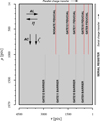 |
Fig. 1 Schematic diagram of one of Gaia’s CCDs, as seen from the illuminated side and showing various features relevant to the PSF modelling. The (τ,μ) coordinates represent positions within the pixel grid. The images of stars move from left to right during integration, with the serial register lying on the right. The main AL and AC directions and their relation to the field angles η and ζ are indicated at the top left. Fiducial lines and barriers for the five longest gates are indicated; NOGATE has no corresponding barrier and uses the entire AL range. |
CCD gate constants.
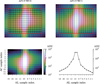 |
Fig. 2 Example window geometry and sampling strategy for a simulated G ≈ 13 source in window class 0 (WC0; upper left) and WC1 (upper right). These particular configurations apply to sources with onboard-estimated G < 13 (WC0) and 13 < G < 16 (WC1), in CCD strips AF2-9. Faint grey lines mark the boundaries between individual samples. The red boxes mark the extent of the window region, with the internal black lines indicating the binning of individual samples. The lower panels depict the resulting downlinked 2D (left) and 1D (right) observations. |
3 Drift-scan mode with precession
The great majority of astronomical telescopes and imaging systems operate as framing cameras in point-and-stare mode, where the telescope is held stationary or tracked to compensate for the rotation of the Earth for example, such that the stars or other objects being imaged remain in a fixed position in the detector during the exposure. This allows the received signal to accumulate in individual pixels. In contrast, Gaia spins continuously during operation such that the images of stars drift smoothly across the focal plane as they are being observed, travelling along the CCDs in almost exactly the direction of the pixel columns at an almost constant rate. At the same time, the accumulating charge is moved through the CCDs at a fixed rate that matches the expected average drift rate of stellar images, with the ~4.42 second crossing time for individual CCDs placing a fixed upper limit on the exposure time for all sources. The combination of a drift-scanning telescope with CCDs operating in TDI mode offers certain advantages over point-and-stare imaging. In particular, many CCD level instrument calibrations collapse from two to one dimension, as the variation in the direction along scan is marginalised. This includes the CCD response, flatfield, background, and geometric calibration. Images are captured as continuous strips of essentially arbitrary length in the direction along scan, which is a useful strategy for survey instruments. For example, this technique is employed by the HiRISE camera on Mars Reconnaissance Orbiter (McEwen et al. 2007) and the Lunar Reconnaissance Orbiter Camera (Robinson et al. 2010), both of which are used to image long continuous swathes of terrain. Drift-scan mode has also been used to great success in other astronomical surveys such as the Sloan Digital Sky Survey (Gunn et al. 1998).
3.1 Stellar image motion
However, the particular drift-scan strategy implemented by Gaia introduces some complications in the PSF modelling. As it spins, Gaia’s rotation axis precesses at a rate of around 4° per day relative to the stars, allowing the whole sky to be observed over a period of around 63 days. The evolution of the spacecraft pointing is known as the Gaia ‘scanning law’ (see Gaia Collaboration 2016b, Sect. 5.2). The precessional motion induces a periodic across-scan motion of stellar images as they transit the focal plane, which causes the integrated images to be smeared out in the across-scan direction. The across scan motion varies sinusoidally in time with a nominal period of six hours (one revolution) and an amplitude of 173 mas s−1, which, given the ~4.42 second integration time and nominal across-scan pixel scale of pμ = 176.8 mas pix−1, implies a maximum smearing of around 4.3 pixels, with the majority of observations smeared across-scan by at least ~3 pixels. This is a major disturbance in the PSF that must be incorporated into the modelling. In Paper I the smearing effect was modelled empirically, by introducing a dependence of the basis component amplitudes on the across-scan rate (see Sect. 4.1 in this paper). This was only partially successful, and major systematic errors remained. As it was noted at the time, this was mainly due to the along-scan rate of stellar images deviating systematically from the charge transfer rate, leading to a shearing effect on the PSF that was not reproduced by the model.
In fact, small but significant differences between the AL image rate and the charge transfer rate are unavoidable, and arise due to several effects. First, the two telescopes have slightly different focal lengths (~34.9708 m for FOV1 and ~34.9688 m for FOV2; see Fig. 4.24 in Hobbs et al. 2022), so the projected images of stars move at slightly different linear speeds on the CCDs even at the same angular rate; the difference is around 0.058 pix s−1, which is equivalent to ~3.4 mas s−1. The spin rate of the satellite is adjusted so that the average of the two FOVs matches the charge transfer rate. Variations in the along-scan pixel scale pτ across the focal plane mean that no single value is appropriate for either telescope anyway. Second, the scanning law itself induces a small sinusoidal variation in η that has a one revolution period and an amplitude of up to ~1.1 mas s−1. This is analogous to the better-known ζ modulation, but out of phase by π∕2 and with a smaller amplitude (see Lindegren 2025b) that varies strongly depending on the CCD row, being largest (and of opposite sign) in rows 1 and 7 and almost zero in row 4. The η variation is due to precession-induced field rotation and not, for example, due to changes in the spin rate of the satellite. The precession rate varies over the year due to the ellipticity of Earth’s orbit and the need to keep the sun at a constant aspect angle. This induces a small annual modulation in the amplitude of the η variation.
Finally, both η̇ and ζ̇ are affected by frequent disturbances in the attitude from a variety of phenomena, including thermomechanical micro-clanks, micro-meteroid impacts, and fuel movements in the propellant tanks. The on-board attitude control system detects and corrects these, but this inevitably leads to short periods where the attitude rate is compromised. In Fig. 3, we show an example of the observed variation in τ̇ and μ̇ in the two fields of view over a period of two revolutions, which is a combination of all of these effects. Any offset from zero means that the stellar image moves relative to the integrating charge, and the resulting integrated image is smeared out along a line determined by the motion in each dimension. In Fig. 4 we demonstrate the apparent shearing effect that this has on the integrated effective PSF, and its dependence on the magnitude and sign of the motion in each of the AL and AC directions. Note that in this work we assume the AC component of the smearing has no effect on the LSF, and that it is sensitive only to T - T0. This is not entirely true: large AC smearing causes minor additional flux loss from the (12 pixel wide) window, which may have a very minor effect on the LSF shape, and signal-level-dependent effects will vary with the AC smearing since this has a significant impact on the pixel occupancy in the core of the charge packet. Both of these effects are very weak, and may be addressed in future PLSF model developments.
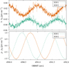 |
Fig. 3 Example of the observed AL (upper) and AC (lower) stellar image drift rates relative to the transferring charge over a two-revolution (12 hour) period, for both FOVs and measured at the centre of a CCD in row 1. |
3.2 Along-scan variations and the ‘corner effect’
In addition to the major smearing effect, the motion of the stellar image relative to the transferring charge packet induces an additional modulation in the resulting integrated image that is subtler. When the stellar image is significantly trailed, different samples in the image are exposed over slightly different ranges of τ, and will therefore have a weak dependence on any spatial variations in the instantaneous effective PSF in the AL direction within the CCD. While purely optical variations in the PSF are generally insignificant over the AL extent of a single CCD, it turns out that the CCDs used by Gaia have a systematic spatial variation in the pixel response non-uniformity that introduces significant AL variation in the electronic component of the PSF, originating in the detector itself. This is ultimately caused by a characteristic circular pattern of thickness variation arising from the way each device was manufactured from either the left or right half of a circular silicon wafer. Thinner regions have a lower quantum efficiency at red wavelengths, resulting in a lower overall response. This is referred to as the ‘corner effect’ elsewhere in Gaia documentation, due to the response being weakest towards the corners where the CCDs are thinnest. This is depicted in Fig. 5. All the CCDs naturally fall into two types depending on whether they were manufactured from the left (TYPE-01) or right (TYPE-02) half of the circular wafer. Across the SM and AF part of the focal plane there are 35 TYPE-01 devices and 41 TYPE-02 devices, as listed in Appendix C. There are also ten pairs of twin devices that have been manufactured from each half of the same wafer; these can sometimes have similar properties. Regardless of type, the devices are always orientated in the focal plane with the serial register on the right. Thinner regions of the CCD have a lower quantum efficiency at red wavelengths, which results in a (polychromatic) PSF that is narrower due to diffraction effects. There may also be some contribution from reduced charge diffusion due to the shorter distance travelled by photoelectrons to reach the electrodes. The main observational consequence of this is that the AL width of the PSF varies as a function of τ. This is clearly visible when inspecting the PSF for different CCD gates, since each gate samples a different range of τ and is subject to a different average CCD response. In Fig. 6 we present the PSF AL full-width half-maximum (FWHM) as a function of CCD gate for two devices of different type. Within each device the behaviour is very similar between the FOVs despite the optical PSFs being very different. However, the devices diverge significantly in their gate-dependent behaviour, since in TYPE-01 devices the pixel response plateaus close to the serial register, so the short gates have similar PSFs, whereas in TYPE-02 devices the pixel response decreases rapidly close to the serial register and successively shorter gates have narrower PSFs.
The consequence of this is that whenever the stellar image is trailed, the integrated effective PSF becomes sensitive to τ variations in the instantaneous effective PSF, which are dominated by the corner effect described above5. This manifests as a characteristic modulation in the PSF that is opposite in sign between the two device types. This is demonstrated in Fig. 7, in which the structure is caused entirely by the dependence of the instantaneous effective PSF on τ. Note that since τ̇ - τ̇0 ≪ μ̇ - μ̇0 this phenomenon has a much weaker impact on the LSF and is not observed in the 1D observations. This dependence is different to the other major PLSF dependences on source colour or μ location for example, since observations are produced by integration over a range of τ and do not sample a single value of it. It is also somewhat unexpected for Gaia, since it contravenes the idea that drift-scan mode marginalises instrumental variations in the along-scan direction. However, it is present in the data and must be accounted for in the PSF modelling.
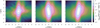 |
Fig. 4 Effects of AL and AC source motion on the PSF. These plots depict the integrated effective PSF for three different regimes of τ̇ and μ̇. The u and v coordinates are relative to the PSF origin, as explained at the start of Sect. 4.1. These plots have been generated using the calibrated PSF model presented later in this paper, and correspond to the FOV1 PSF for NOGATE observations in the ROW2 AF4 device. In the left panel τ̇ = τ̇0 and μ̇ = μ̇0 such that the stellar image motion is perfectly matched to the charge transfer and no smearing occurs in either dimension. In both the centre and right panels τ̇ - τ̇0 = 0.226 pix s−1, such that the stellar image lags one pixel behind the charge in the AL direction during the 4.42 second exposure. In the centre and right panels μ̇ - μ̇0 = 0.974 and −0.974 pix s−1 respectively, such that the stellar image moves ±4.3 pixels in the AC direction, orthogonally to the charge transfer. Note that the τ̇ value is about 20 times larger than what is routinely observed in the real data, in order to make the impact on the PSF more obvious for the plots. Throughout this paper we make use of the cubehelix colour scheme introduced in Green (2011). |
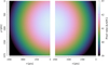 |
Fig. 5 Illustrative example of (artificial) flatfield images for a pair of CCDs manufactured from the same circular silicon wafer. This figure approximately reproduces the effect seen in industrial pre-launch flatfield data from Gaia’s CCDs at 900 nm, and which cannot be published. The CCD on the left is of TYPE-01 and the CCD on the right is of TYPE-02. |
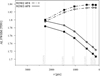 |
Fig. 6 Effects of AL variations in the CCD response on the PSF, and the dependence on CCD gate and device type. The AL FWHM of the integrated effective PSF is plotted as a function of CCD gate, for two devices of TYPE-01 (ROW2 AF4, dot-dashed line) and TYPE-02 (ROW3 AF9, solid line). Each CCD gate spans a range in τ, with the points plotted at the fiducial line positions. The solid squares correspond to FOV1 and the open circles to FOV2. These figures have been generated using the calibrated PSF model rather than directly from the observations. |
4 Brief review of the EDR3 PLSF models
In this section, we present a brief review of the PSF and LSF models implemented for Gaia EDR3, in order to introduce some notation and provide context for the improvements presented in this paper. Further details can be found in Sect. 3 of Paper I, although note that some of the nomenclature has been updated for the present paper.
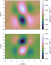 |
Fig. 7 Effects of AL variations in the CCD response on the PSF, and the dependence on source motion. Each plot shows the difference between two integrated effective PSFs for τ̇ = τ̇0 and μ̇ - μ̇0 = ±1.0 pix s−1, such that the PSFs are smeared exclusively in the AC direction. The PSFs are for NOGATE, so the entire τ range of the CCD is covered. Due to the AC motion, the lower half of each plot shows the approximate difference between the instantaneous effective PSF at high τ minus the instantaneous effective PSF at low τ, and vice-versa in the upper half. The lower panel is a TYPE-01 device (ROW2 AF4) and the upper panel is a TYPE-02 device (ROW3 AF9). |
4.1 The EDR3 PSF model
The PSF model P predicts the fractional charge contained in a sample located at (u, v) relative to the PSF origin. The u and v axes are aligned with the AL and AC directions, and oriented such that v increases in the direction of increasing μ, and u increases in the direction of increasing observation time6. Note that u is formally in units of the TDI period, denoted TDI1, and v is in units of pixels. P is dependent also on the effective wavenumber7 νeff, the AC position in the device8 μ, and the AC rate μ̇. No correction for the native AC rate μ̇0 was required. Interpreted as a probability density function conditional on the νeff, μ, and μ̇ variables, it can be written P(u, v|νeff,μ,μ̇). The PSF model is composed as the linear combination of a 2D mean PSF, denoted G0, and N weighted basis components, denoted Gn, with associated weight factors gn and N = 30 in EDR3. The full expression for the PSF model is written
 (2)
(2)
The mean PSF G0 is normalised such that its integral over all (u, v) is 1.0, and it has a fixed weight of 1.0. The other components are normalised such that their integrals over all (u, v) are 0.0. This guarantees that the full PSF model is normalised to 1.0 regardless of the weighting of the components. The basis components are by construction mutually orthogonal as far as possible (though see Sect. 5.1.3), which improves numerical stability and ensures a unique solution. The weight factors gn (νeff,μ,μ̇) are represented as multi-dimensional splines in the dependent variables (using the implementation described in van Leeuwen 2007, Appendix B, extended to multiple dimensions), with appropriately configured spline orders and knot sequences in each dimension. The full set of spline coefficients over all N basis components defines the complete set of parameters of the PSF model.
The G0 and Gn functions are constructed as the linear combination of outer products of 1D basis functions in the AL and AC direction, denoted fi and hj, where i and j index functions of different order in each dimension9, so that
 (3)
(3)
with I = 21 and J = 21 in DR3. Each product fi(u)hj(v) is referred to as a ‘pseudo shapelet’ (to distinguish it from the shapelets model presented in Refregier 2003) and the full model was named ‘compound shapelets’ in Paper I. The (constant) matrix  defines the construction of G0 and Gn from linear combinations of the 1D functions of order i and j. The functions f and h are physically motivated, and are derived in advance from simulations of Gaia’s optical system as described in Lindegren (2009). They account for pixelisation in each dimension and are represented using the S-spline function presented in Castañeda et al. (2022, Sect. 3.3.5). The S-spline is formulated to satisfy the shift-invariant-sum requirement, which expresses the conservation of flux under sub-pixel shifts of the source, and is important for the photometry. The matrix α is then obtained by training on real Gaia observations using the principal components analysis algorithm described in Lindegren (2010). This produces G0 and Gn functions that are tailored to the in-flight PSF, and which for a limited number (N = 30) of components provides the smallest expected RMS error among all linear models.
Finally, while the true PSF is strictly positive everywhere, this property is not enforced in our model either by construction or by the calibration of the parameters. As such, it represents a noisy estimate of the true PSF and may be negative at locations where the true PSF is very small, or in poorly constrained regions of the parameter space. It is expected that users of the model within DPAC handle these (rare) situations appropriately.
4.2 The EDR3 LSF model
The LSF model is denoted L, and is composed as the linear combination of a 1D mean LSF, denoted H0, and N weighted basis components, denoted Hn, with associated weight factors gn and N = 25 in EDR3. It is analogous to the PSF model but spans only the AL dimension. As such, it is a function only of the u coordinate, and the dependent variables do not include the AC rate. The full expression for the LSF model is written
 (4)
(4)
In EDR3 the 1D functions H are identical to the f functions derived from simulations, i.e. without training them on real Gaia observations, so H0 ≡ f0, H1 ≡ f1 etc. This was found to be sufficient for EDR3. However, in principle they could be composed of linear combinations of f in order to tailor them to the in-flight LSF modes, so that for example
 (5)
(5)
This was not done in EDR3 but is in DR4, so we prefer to use the H symbol to generalise the model.
5 The DR4 PLSF model
The PLSF models used in DR4 have undergone several major advances relative to the EDR3 models presented in the previous section. Here we present a complete derivation of the updated models, the calibration algorithms used in the operational processing and the PLSF configurations chosen for modelling different subsets of the data. Note that we also updated and improved the LSF and PSF basis components H and G, the 1D functions f and h used to compose them, and the fundamental S-spline function used to interpolate f and h. These are somewhat secondary to the PLSF models themselves, and their presentation is deferred to Castañeda et al., (in prep., Sect. 3.3.5).
5.1 Derivation of the DR4 PLSF models
In this section we describe three major advances in the PLSF model, which are the switch from a limited (AC-only) empirical model of the source motion to a complete (AL and AC) analytic model (Sect. 5.1.1), the incorporation of a crucial dependence on TDI line number (Sect. 5.1.2), and the introduction of constraints between the PLSF origin and the geometric instrument calibration (Sect. 5.1.3). The complete derivation is presented in terms of the PSF model; the updated LSF model, to which only a subset of these effects apply, is presented briefly in Sect. 5.1.4.
5.1.1 Analytic modelling of the AL and AC source motion
The EDR3 PSF model included a limited modelling of the source motion through the dependence of the basis component amplitudes gn on the μ̇ parameter, which was in turn parameterised Article number, page 8 of 27 using a third order polynomial (see Table 3 in Paper I) with coefficients calibrated empirically by fitting to observations. Unlike the other empirically calibrated dependences (on νeff and μ) the effects of AL and AC source motion can be modelled from first principles as a simple smearing of the integrated PSF along the direction of motion. The first step is to remove μ̇ from the dependent variables in Eq. (2) to obtain
 (6)
(6)
By substituting the expressions for G0 and Gn from Eq. (3) and specifying g0(νeff,μ) = 1,  , and
, and  , we obtain an expression directly in terms of the 1D functions fi and hj:
 (7)
(7)
where I = 25 and J = 25 in DR4. We now introduce a new variable τ that represents the TDI line number during the exposure, and introduce correction terms to u and v that represent the displacement of the stellar image from the charge image as a function of τ and the field angle rates η̇ and ζ̇, to obtain an expression for the instantaneous effective PSF at TDI line number τ:
 (8)
(8)
The displacement terms ∆u(τ, η̇) and ∆v(τ, ζ̇) have the following forms, making use of the expressions in Eq. (1) and the exposure time, texp:
 (9)
(9)
 (10)
(10)
where the sign change in Eq. (9) reflects the fact that the AL direction is opposite to the direction of increasing η. In these expressions ∆τ = τmin − τmax, where τmin and τmax are the minimum and maximum value of the TDI line number. The value of τmax depends on the CCD gate used to observe the source, with longer gates having a larger value. In contrast, τmin has the same value of 1 for all gates, corresponding to the final TDI line before the serial register is reached. In adopting this value, we ignored the fact that TDI lines 1, 2, 5, 6, 9, and 10 are masked and are not light sensitive; as the AL and AC motion is very small over such a short extent the impact of this approximation is insignificant10. The quantity τF is the TDI line number of the CCD gate fiducial line, which corresponds to the mean of the light sensitive TDI lines and is slightly more than half of τmax due to the 6 masked TDI lines. τf is the reference coordinate used in the astrometric solution, and for the purposes of modelling the PSF we define the displacement of the stellar image away from the integrating charge image to be zero at τF. The values of τmax, τF, and texp for all gates routinely in use is listed in Table 1. The instantaneous effective PSF is never actually observed, and in order to model the PSF for a particular observation we compute the integrated effective PSF by marginalising the nuisance parameter τ:
 (11)
(11)
The integration limits depend on the CCD gate of the observation according to Table 1. Note that the integral range is reversed, to reflect the sense of the TDI line coordinate on the device: exposure starts at high TDI line number and ends at low TDI line number. We use the optimisation  to eliminate the summation over n since gn has the same value for all (u, v) samples in the PSF model for a particular observation. This results in the expression
 (12)
(12)
Note that the computation can be further optimised by caching and reusing the sampled values of fi(u + ∆u(τ, η̇)) and hj(v + ∆v(τ, ζ)) when the (u, v) locations fall on a regular grid, which occurs in routine processing when a 2D window is being modelled. The integration is performed numerically using Gauss-Legendre quadrature, according to which the integral becomes a weighted sum over K steps in the τ coordinate,
 (13)
(13)
where the leading ∆τ factor is absorbed into the weights wk. This is the equation that is implemented in the Gaia data processing and used to model the PSF for observations in GATE4 to GATE9, for which the dependence of the PSF shape on τ can be ignored (order = 1 in Table 1). We selected K = 9 as an optimal tradeoff between numerical accuracy and execution time; for details of the numerical integration, values of the wk weight factors and their associated τk coordinates; see Appendix D. The first derivatives of the PSF model with respect to the u and v parameters are required when fitting the model to an observation; these have the simple forms
 (14)
(14)
and
 (15)
(15)
where the prime denotes the first derivative. Finally, when the exposure time or either of the η̇ and ζ̇ terms are very small11 the corresponding ∆u and/or ∆v terms in Eq. (12) are eliminated. These conditions are met for very short gates or observations whose AL and AC motion is closely matched to the charge transfer. In these circumstances the integration is either avoided entirely or can be performed by analytic integration of whichever of the fi or hj functions still retain a dependence on τ. Recall that these functions are represented using the S-spline described in Castañeda et al., (in prep., Sect. 3.3.5), which is ultimately based on b-splines and can be integrated analytically.
5.1.2 PSF dependence on TDI line number
As explained in Sect. 3.2, spatial variations in the PSF shape within each device are not restricted to the AC direction (parameterised by μ), and the variation in the AL direction, parameterised by the TDI line number τ, is also significant. The dependence on τ is similar in principle to the dependences on μ and νeff, with the important difference that individual observations span a range in TDI line number during exposure rather than a single value. This can be incorporated into our model by expanding the parameterisation of the weight factors gn to include τ, so that they are modified to

Under this approach, the instantaneous effective PSF (Eq. (8)) is modified to
 (16)
(16)
The expression for the integrated effective PSF (Eq. (11)) is adjusted to bring the weight factors inside the integral, since they now depend on τ. Applying the Gauss-Legendre quadrature scheme, and redefining β to include τ so that βij(νeff,μ, τ) =  , we finally obtain the expression
 (17)
(17)
This is the equation that is implemented in the Gaia data processing and used to model the PSF for observations in GATE10 to NOGATE, for which the dependence of the PSF shape on τ cannot be ignored (order > 1 in Table 1). The first derivatives with respect to the u and v parameters can be formed in the same way as for Eq. (13), i.e. by replacing the f and h functions with their first derivatives, respectively. The need to compute β at each of the K numerical integration steps leads to a modest drop in computational performance relative to Eq. (13), and the dependence of β on τ means that the numerical integration cannot be avoided in situations where the ∆u or ∆v factors are eliminated.
Observations for which ∆u and/or ∆v are close zero, i.e. when |τ̇ - τ̇0| or |μ̇ -μ̇0| are small, offer little constraint on the τ dependence in β. This has some implications for the calibration. For example, during the first month or so of science data collection Gaia followed the Ecliptic Pole Scanning Law, in which the μ̇ distribution of the observations is around four times narrower than the Nominal Scanning Law. This led to a somewhat underconstrained τ dependence in the longer gates over revolutions 1078 to 1192, which required some adjustments in the calibration pipeline during the late stages of the data processing for DR4. Finally, we note that it would in principle be possible to obtain the model for a short gate observation by integrating the model for a longer gate over a restricted range in τ. This was considered but not explored in depth.
5.1.3 Constraints on the PLSF origin
In the context of the Gaia global astrometric solution there is a degeneracy between the PLSF origin and the geometric instrument calibration, the latter being solved separately to the PLSF as part of the AGIS processing (see Lindegren et al. 2012, Sect. 3.4). In the complete instrument model, purely optical shifts in the PLSF origin, caused for example by evolving wavefront tip-tilt or ice contamination, are indistinguishable from physical displacements of the devices. Breaking this degeneracy is vital to separate the roles of the different calibrations. This is done by enforcing some constraints on the origin of the PLSF model, as explained in this section.
Up to this point the PLSF origin has not been explicitly defined, and is by default coincident with the origin of the 1D functions f and h. Early representations of the Gaia LSF included a translation parameter applied to the sample location, allowing the LSF model to shift by an arbitrary amount in the AL direction (see Paper I Sect. 6.7.2). In the present paper we generalise this idea to the PSF, and introduce u0 and v0 to denote the shifts of the PSF in the AL and AC direction. To incorporate these parameters in the PSF model, we first modify Eq. (6) to
 (18)
(18)
Before DR4 the u0 and v0 parameters were implicitly fixed at zero, with small shifts of the PLSF origin handled by appropriate weighting of the basis components. This is undesirable for two reasons. First, it requires the basis components to reproduce pure shifts of the PLSF, which increases the dimensionality. Second, it precludes the explicit calibration of the PLSF shifts, which is necessary in order to break the degeneracy with the geometric calibration. Therefore, in the DR4 PLSF model we treat u0 and v0 as free parameters and make an explicit calibration of them. Like the other PSF parameters they have dependences on νeff and μ, so u0 ≡ u0(νeff,μ) etc. However, the introduction of u0 and v0 is a major inconvenience for the PLSF calibration because Eq. (18) is non-linear in terms of these parameters, for example  . This requires the fitting to be iterated, and complicates the implementation of the running solution that is used to account for variation with time. Instead, we adopted the following linearised form of the model
 (19)
(19)
which is derived from Eq. (18) by Taylor expansion, ignoring terms of order O(u0gn) and O(v0gn) and higher (Lindegren 2025a). This form of the model is much more convenient as it can be made equivalent to Eq. (6) by representing the derivatives of G0 as linear combinations of the pseudo shapelets (Eq. (3)) and introducing them as additional basis components with amplitudes −u0(νeff,μ) and −v0(νeff,μ). In this formulation we have the identities
 (20)
(20)
The basis components G1 and G2 and their amplitudes g1 and g2 therefore model small shifts of the PSF origin in the AL and AC directions, whereas the basis components G3+ and their amplitudes g3+ model the shape of the PSF. In order to guarantee the independence of the shift and shape parameters the basis components G must be mutually orthogonal. This is enforced during the production of the basis components: once the mean PSF G0 and the first derivatives G1 and G2 are established, the higher order basis components G3+ are post-processed to subtract their projections onto G1 and G2 in a process of Gram-Schmidt orthogonalisation, i.e.
 (21)
(21)
for n ≥ 3. These steps are ultimately carried out by manipulating the elements of the matrix  . The resulting PLSF basis components are presented in Castañeda et al., (in prep, Sect. 3.3.5.2).
The explicit calibration of the PSF shifts can now be used to break the degeneracy with the geometric instrument calibration. This involves shifting the PSF model by correcting the g1 and g2 terms by their values at the reference wavenumber  , where
  . In practice this amounts to making the transformation
 (22)
(22)
and then using g′1 and g′2 in the PSF model. Note that this step is only applied during Astrometric Detection and Image Parameter Determination (DIPD; see Castañeda et al., in prep., Sect. 3.3.7) when the PSF model is used to estimate the locations of sources in the Gaia data stream12; formally, the estimated locations are defined as relative to the location of an equivalent source with  . This procedure is referred to elsewhere in Gaia documentation as the non-chromatic constraints—see Lindegren (2025a) for further details13. Finally, when the PSF model includes a dependence on TDI line number τ such that g1 ≡ g1(veff,μ,τ) for example, then the constraints in Eq. (22) are adjusted to
 (23)
(23)
i.e. we use the value of the shift at the CCD fiducial line τF.
Note that there are several known limitations in this model that complicate its use. First, the linearised form of the model in Eq. (19) is a truncated expansion and is only valid for relatively small values of u0 and v0. Second, the mean PSF G0 may not be accurate for a given CCD and/or time. Finally, structure in the PSF prevents G1 and G2 from being fully orthogonal. These imply that the calibration of the PSF shift and shape are not fully decoupled, and that the g1 and g2 parameters absorb a small amount of shape change, and vice-versa. The application of the non-chromatic constraints then results in some undesired change in the PSF model shape, degrading the IPD performance. However, successive iterations of the PSF calibration and global astrometric solution drive the correction terms  and
and  towards zero, which eliminates this problem.
5.1.4 The DR4 LSF model
The vast majority of Gaia observations are 1D and are modelled using the LSF. The marginalisation of the AC dimension greatly simplifies the modelling by reducing the dimensionality and eliminating (to a very good approximation) the dependences on AC rate and TDI line number. The LSF model developed for DR4 can be derived from the EDR3 model presented in Eq. (4) by applying a similar derivation as to the PSF, albeit simpler, and making use of the relations in Eq. (5) to first write down the instantaneous effective LSF,
 (24)
(24)
where  , and with the identities g0(veff,μ) = 1,
  , and
, and  . As for the PSF, the matrix α is constant and defines the construction of the N 1D basis components from linear combinations of the 1D functions f. To generate the model for a particular observation we integrate over τ to obtain the integrated effective LSF,
 (25)
(25)
The 1D observations always use NOGATE14, so τmin = 1 and τmax = 4500 according to Table 1. The integration now accounts solely for the smearing in the AL direction, and is equivalent to a convolution of fi with a top hat of width |(τ − τ0) texp| and amplitude |(τ̇ - τ̇0)texp|−1 centred on the origin. In the case of the LSF this integration can be computed analytically, which avoids the need to adopt the Gauss-Legendre quadrature scheme necessary for the PSF. The LSF model is also invariant to changes in the sign of (τ̇ - τ̇0), which is not the case for the PSF model.
Note that the LSF origin is calibrated in the same way as for the PSF, as described in Sect. 5.1.3. Briefly, the N 1D basis components are constructed (via the elements of α) such that component n = 1 is the derivative of the mean (n = 0), with the n = 2+ components being orthogonalised in order to separate the parameters of the LSF into shift (g1) and shape (g2+) terms. When using the LSF to measure AL locations of observations we correct the g1 term as shown in Eq. (22).
5.2 Calibration algorithm
The PLSF models described above are calibrated for use in the science data processing using regular science observations, specifically windows containing single isolated stars, rather than any dedicated calibration data. The eligibility, selection and preprocessing of the windows follows the same basic procedure as described in Paper I Sects. 4.1 and 4.2, and will not be repeated here. A few minor improvements and adaptations to the new calibration models have been made; these will be described in detail in Castañeda et al., (in prep.). Note that while time variation in the PLSF is very significant over the course of the mission, due to varying levels of ice contamination, focus evolution, thermal instabilities and other factors, the PLSF models presented here contain no time dependence. Instead, the evolving state of the instrument is tracked by making independent ‘partial solutions’ for all 1268 PLSF calibration units for every one revolution (~6 hour) interval throughout the mission. These partial solutions, which may not be well constrained over the whole parameter space, are then smoothed using a square root information filter. This improves constraint while allowing gradual time evolution in the solution, albeit with small discontinuities between consecutive revolutions. This is the same ‘running solution’ methodology used in the DR3 processing, and which is described in Paper I Sect. 3.4.5. For DR4 we increased the time interval for the partial solutions from 0.5 to 1.0 revolution, mainly to reduce the data volume, and reduced the time constant in the filter from 80 revs−1 to 40 revs−1 for the PSF and 20 revs−1 for the LSF, in order to better track rapid changes. The trending over time is not explored further here, and instead we present the updated calibration equations for the partial solution, which have been revised considerably since DR3 due to the new PLSF model formulation. We focus on the construction of the design matrix based on the relations between individual calibration samples and the coefficients of the PLSF models.
The weight factors gn are modelled using multi-dimensional splines in (νeff,μ,τ) or (νeff,μ), depending on the type of model. We include the τ dependence in the presentation that follows. The spline value is computed as the inner product of the P spline parameters a, where
![Mathematical equation: \vec{a}^T=[a_1, a_2, \ldots, a_P] ,](/articles/aa/full_html/2026/04/aa58618-25/aa58618-25-eq42.png)
and the spline coefficients y(νeff,μ,τ), where
![Mathematical equation: \vec{y}(\nu_{\text{eff}},\mu, \tau)^T=[y(\nu_{\text{eff}},\mu, \tau)_1, y(\nu_{\text{eff}},\mu, \tau)_2, \ldots, y(\nu_{\text{eff}},\mu, \tau)_P] ,](/articles/aa/full_html/2026/04/aa58618-25/aa58618-25-eq43.png)
so that for example

By convention, the spline coefficients are determined by the spline configuration (the knot sequence and polynomial order) and the coordinate (νeff,μ,τ), while the spline parameters are the quantities solved for when fitting the spline to observations. In this work we adopted the spline implementation described in Appendix B of van Leeuwen (2007), generalised to multiple dimensions. The weight factor associated with each basis component has an independent set of parameters, and in general may use a different spline configuration and therefore have a different number of parameters, so that P ≡ Pn. The full set of parameters for the PSF model can be represented in a single column vector x as
![Mathematical equation: \vec{x}^T = [\vec{a}_1^T, \vec{a}_2^T, \ldots, \vec{a}_N^T] ,](/articles/aa/full_html/2026/04/aa58618-25/aa58618-25-eq45.png)
where an contains the Pn spline parameters corresponding to the weight factor gn, with corresponding coefficients yn. Note that n = 1,2,..., N and that the amplitude of the mean (n = 0) is fixed at 1.0 and excluded from the calibration. The pth spline parameter for the nth weight factor is denoted  , with corresponding coefficient
  .
.
The calibration algorithm involves solving for the parameters x that provide the best fit to the observations in a least squares sense. This can be expressed in the usual manner as a system of linear equations
 (26)
(26)
where the vector b contains all of the observations used to constrain the PSF model. The observations correspond to individual samples drawn from carefully selected and preprocessed windows, and are normalised by the source flux. The windows are indexed using m, where m = 1,2,..., M. Each window has an associated source colour νeff,m, AC position μm and field angle rates η̇m and ζ̇m, and provides multiple individual samples s that are indexed using r, where r = 1,2,...,R. Each sample has an associated location relative to the PSF origin, denoted (ur, vr), which is obtained from the predicted location of the source15 in the window and the position of the sample. The vector b can therefore be written as ![Mathematical equation: $\vec{b}^T=[\vec{s}_1^T, \vec{s}_2^T, \ldots, \vec{s}_M^T]$](/articles/aa/full_html/2026/04/aa58618-25/aa58618-25-eq49.png) where sm represents the R samples from window m, and
where sm represents the R samples from window m, and ![Mathematical equation: $\vec{s}_m^T=[s_m^1, s_m^2, \ldots, s_m^R]$](/articles/aa/full_html/2026/04/aa58618-25/aa58618-25-eq50.png) where
where  represents the rth sample from the mth window. Finally, the mean G0 is subtracted from each sample; as the amplitude of the mean is fixed at 1.0 it is excluded from the fit, and only the amplitudes of the basis components are solved for by fitting to the sample residuals. In terms of these quantities, the complete model for each sample is constructed as

The rows of the design matrix A are indexed by m, r and the columns are indexed by n, p. The element with indices m, r, n, p is constructed

This is used to construct the design matrix in the calibration of the PSF model in Eq. (17), in which the PSF shape has an explicit dependence on τ. The variant of the PSF model presented in Eq. (13) has no explicit dependence on τ, and the corresponding expression for the design matrix elements is

Finally, the LSF model presented in Eq. (25) has the following expression for the design matrix elements:

Each element in b and the associated row in the design matrix are weighted by the uncertainty on the observation, which is estimated assuming Poisson statistics and accounting for the uncertainties in the various auxiliary calibrations. The solution for the parameters x is obtained by applying Householder orthogonal transformations to Eq. (26) that reduces matrix A to a particular upper triangular form. For further details, see van Leeuwen (2007, Appendix C) and Bierman (1977, chapter 4). We also obtain the formal uncertainty on the parameters solution in terms of the square root of the covariance matrix, denoted Ux (based on the notation from van Leeuwen 2007), which can be used to obtain by transformation the covariance matrix for the PLSF model samples associated with a particular observation.
5.3 Configuration
The configuration of the PLSF models refers to the choice of the number of basis components and the configuration of the multi-dimensional splines used to interpolate the amplitude of each component independently, as well as the range for each dimension. In Tables 2 and 3 we present the configurations of the main LSF and PSF dependences that were selected for operational use; we find that splines of low order16 in each dimension are generally sufficient for the majority of observations, with only the νeff dimension requiring a single internal knot (although see Sect. 7.2 for further discussion). This was largely determined empirically through trial and error, although AGIS requires that the shift parameters have a linear dependence on νeff with no knots (see Lindegren 2025a, Sect. 7.1), which explains why the g1 and g1,g2 functions have separate entries. The range of μ and τ are determined by the CCD light sensitive area and gate length. Recall from footnote 8 that for practical reasons we use the μ of the window centre rather than the source within it; this is a good enough estimate. The νeff range of 1.08 ≤ νeff ≤ 1.9 μm−1 spans the vast majority of stars17, and corresponds roughly to −0.53 ≤ GBP - GRP ≤ 7.6 according to E.4 in Lindegren et al. (2021). Sources with νeff lying outside of this range are not used in the PLSF calibration, and their observations are processed using the PLSF model for the closest limiting value (1.08 or 1.9 μm−1 ), a procedure referred to as ‘clamping’ the νeff. None of the other empirically calibrated dependences require this intervention. The combination of the number of basis components and the spline configuration determines the total number of free parameters in the model. For the LSF model we use 25 1D basis components (N = 25) which corresponds to 294 free parameters per calibration unit. This is reduced to 17 basis components and 198 free parameters for the calibration units corresponding to the AF1 CCD strip; these use shorter windows that require fewer bases. For the PSF model we use 30 2D basis components for all calibration units. This corresponds to 348 free parameters for the calibration units with no τ dependence, which are those that use CCD gates 4, 7, 8, and 9 in AF, and all the WC1 calibration units in SM. Calibration units with a linear τ dependence (gates 10 and 11) have 696 free parameters, and those with a quadratic τ dependence (gates 0 and 12, including SM WC0) have 1044 free parameters.
Each of the 1268 calibration units in the SM and AF focal plane has a dedicated LSF or PSF model that is solved independently, with two minor exceptions. The WC2 LSF solutions in AF (i.e. corresponding to 1D observations with G ≳ 16) are discarded and replaced with the corresponding WC1 solutions (calibrated using 13 ≲ G ≲ 16 observations) from the same device and FOV, and the WC1 PSF solutions in SM (i.e. corresponding to 2D observations with G ≳ 13) are discarded and replaced with the corresponding WC0 solutions (calibrated using G ≲ 13 observations) from the same device (each SM device observes only one FOV) but with the dependence on τ eliminated. The motivation for these choices is that in both cases the PLSF dependences are expected to be the same, since the observations use the same CCD area and FOV and no magnitude dependent effects are currently included in the model, and the brighter observations allow a higher signal to noise solution. The τ dependence is eliminated in the SM WC1 model for performance reasons and because the larger sample binning of the WC1 data (4 × 4 pixels) makes the effects much weaker. Note that in EDR3 the SM calibrations were discarded entirely (see Sect. 5.3 in Paper I); for DR4 we now achieve an independent calibration of the SM PSF.
Finally, all of Gaia’s nominal SM and AF science observations correspond to one of the 1268 calibration units, and have a logical choice of PLSF model to use in the processing. However, a small fraction of observations are captured in non-nominal circumstances, for which there is no obvious choice of PLSF. For example, 1D windows are occasionally observed with a CCD gate activated, which can occur when the transit of a faint source coincides with that of a bright source in the same CCD. Indeed, different AL samples in a single window may have used different gates. In dense regions a 1D window may be wholly or partly truncated in the AC direction (i.e. have AL samples that summed fewer AC pixels than expected) if it overlaps with a neighbouring window, resulting in 1D AL samples that enclose different fractions of the AC flux distribution. Other non-nominal situations can arise given the complexity of Gaia. These problematic observations are not used in the PLSF calibration, and the resulting PLSF models are not strictly applicable to them. In some cases it may be possible to assemble a suitable approximate model for the observation from one or more of the nominal PLSFs. However, their processing by downstream systems within DPAC differs depending on the particular requirements of the task, and is not documented here.
Spline configuration for 1D LSF dependences.
Spline configuration for 2D PSF dependences.
5.4 Covariance propagation algorithm
In some circumstances it is useful to obtain estimates of the uncertainty on the model PLSF samples by propagation of the formal uncertainty on the parameters solution. In poorly constrained regions of the parameter space, for example at extreme values of the effective wavenumber or large distances from the PLSF origin, the uncertainty on the PLSF model can be significant. This should in principle be accounted for when performing statistical tests, such as when assessing the goodness-of-fit of the PLSF model to a particular observation. Note that while the errors on the observed samples arising from Poisson fluctuations are uncorrelated (ignoring effects of photon transfer curve non-linearity, e.g. Antilogus et al. 2014), the uncertainties on the model PLSF samples from propagation of the formal calibration uncertainty can have significant non-zero covariance terms.
The following derivation is presented in terms of the PSF model, and includes the τ dependence. The derivation for the LSF model can be obtained in a similar fashion. The formal uncertainty on the PSF model parameters x is represented by the covariance matrix Σx, where  and Ux is the square root of the covariance matrix as explained in Sect. 5.2. Using this to estimate the uncertainty on the PSF model samples involves two steps. The first is to transform the covariance from the PSF model parameters space x to the basis component amplitudes space g, given the (νeff,μ, τ) values of the observation being modelled. This is done according to the standard tensor transformation law
 (27)
(27)
where Σg is the covariance matrix for the basis component amplitudes. The transformation matrix Y contains the spline coefficients for each basis component at the observation parameters (νeff,μ, τ), and has the structure
 (28)
(28)
The sparsity of Y can be exploited to compute Eq. (27) in an efficient manner.
The next stage is to transform the covariance matrix for the basis component amplitudes Σg to the space of the PSF model samples, given the set of (u, v) sample locations. We denote the resulting covariance matrix Σp, and it is computed by
 (29)
(29)
The transformation matrix G contains the values of each basis component at each of the sample locations, and it has the structure
 (30)
(30)
where
 (31)
(31)
In implementation it is usually more efficient to perform these two stages separately (Σx → Σg → ΣP), because iterative fitting of the PSF to an observation involves updating the matrix G while keeping the matrix Y constant. However, the transformations can be combined as follows:
 (32)
(32)
Finally, the TDI line dimension must be integrated over. This is implemented using the same quadrature scheme as before, where we perform a summation over the K TDI line steps τk with associated weights wk. Note that both the matrices G and Y depend on the TDI line number τk and are brought inside the sum. The full equation for the covariance matrix of the PSF model samples is therefore
 (33)
(33)
However, note that in the calibrations carried out for DR4 we found that the formal uncertainty, quantified via ΣP, was much smaller than the remaining systematic errors in the PLSF models, and was therefore not a useful estimate of the true uncertainty. ΣP is also very time consuming to process for every observation, and it could not fit into the available computing resources. For these reasons, the data processing for DR4 made no use of the PLSF model covariance information during IPD, and this section is included for the sake of completeness and in case the covariance information is used in future data processing.
6 Results
In this section, we present some results of applying our PLSF models to real Gaia observations from the DR4 input data. This is a very rich and varied dataset, and there are many different PLSF configurations and calibration units to choose from. We can only show a limited selection, and our focus is on demonstrating the new features of the PLSF models described in this paper, the reduction of systematic errors in the reconstruction of the observations, and improvements in the estimated source locations relative to the previous PLSF models that were applied in DR3. Improvements in the derived Gaia DR4 data products, particularly the source astrometry and G-band photometry, will be deferred to other papers and/or the official documentation. Due to many updates in the production of these data relative to DR3 it is impossible to isolate the changes associated purely with the improved PLSF modelling. We also defer to the official documentation any discussion of the time evolution and overall performance of the PLSF modelling over the complete DR4 data.
We selected Gaia observations over the on-board mission timeline (OBMT) range 4400 to 4410 revolutions18, which is a stable period of good image quality and low ice contamination. Each observation corresponds to a window containing a single, isolated star that has been prepared for use in the PLSF calibration as described in Sect. 4.1 of Paper I (with minor improvements in the background subtraction and uncertainty estimation). For each observation, the predicted location within the window and the field angle rates were obtained from an intermediate astrometric solution (AGIS-4.1) generated as part of the iterative calibrations carried out during the production of DR4 (see Hernández et al., in prep.). In some examples we also make use of the official PLSF calibrations (ELSF-4.2). Other examples involve refitting the model with different configurations in order to demonstrate certain features; these are standalone calibrations produced only for the purposes of this paper.
6.1 AL and AC source motion in 1D and 2D observations
In Fig. 8, we present the model PSF for one particular calibration (FOV1 ROW1 AF6 NOGATE at revolution 4400) and two configurations of τ̇ − τ̇0 and μ̇ - μ̇0 that are commonly encountered in the data, with τ̇ - τ̇0 = 0.045 pix s−1 and μ̇ - μ̇0 = ±0.975 pix s−1. The νeff and μ parameters are set to nominal values of 1.5 μm−1 and 1000 pix respectively. These PSFs are roughly representative of observations captured three hours apart, when the AC rate has changed sign but the AL rate is the same. The two PSFs are related by a shearing effect that is apparent when their difference is plotted. For completeness we include a panel depicting the equivalent effect directly in the observations. This figure is related to figure 22 in Paper I, which presented the effect as an example of a feature missing from the EDR3 PSF model. This effect is now fully incorporated in the PSF model for DR4.
In Fig. 9, we present the model LSF for one particular calibration (FOV1 ROW3 AF5 NOGATE at revolution 4400) and four values of τ̇ - τ̇0 that are representative of the range of values encountered in the data. Recall that the LSF model is invariant to a change in sign of τ̇ - τ̇0, so we plot only the positive values. The νeff and μ parameters are set to nominal values of 1.5 μm−1 and 1000 pix respectively. A non-zero value of τ̇ - τ̇0 causes a smearing of the LSF that is symmetric about the origin. The overall impact on the LSF is smaller than for the PSF due to the lack of additional dependences on μ̇ and τ. While the effect of τ̇ - τ̇0 variation in the model LSF is the same for all CCDs etc, different regions of the focal plane observe quite different distributions in τ̇ - τ̇0 due to the varying amplitude of the scan law contribution, which is maximum in rows 1 and 7 and minimum in row 4. In Fig. 10, we present the residuals to the LSF model for 1D observations in FOV1 ROW7 AF5 NOGATE over revolutions 4400-4410, using both a fixed median value of τ̇ - τ̇0 to compute the LSF model for all observations, and the correct perobservation value. In the latter case the residuals are reduced in size and show much weaker dependence on τ - τ0, indicating that the effect is successfully reproduced by the model. The remaining structure in the residuals is likely due to a combination of several unmodelled effects that are known about and described in Sect. 7.3.
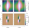 |
Fig. 8 Reproduction of the effects of AL and AC source motion in the PSF model. The upper two panels show two model PSFs that are identical apart from the configured AL and AC source motion: in both cases τ̇ - τ̇0 = −0.045 pix s−1 while μ̇ - μ̇0 = −0.975 (left) and 0.975 (right) pix s−1. The lower left panel shows the difference between the two, which is dominated by the reversed sign of the shearing effect due to the change in sign of the AC rate. The lower right panel depicts the equivalent effect seen directly in the data, and is produced by stacking many observations at μ̇ − μ̇0 > 0.975 and μ̇ - μ̇0 < -0.975 pix s−1 and plotting the difference. |
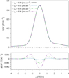 |
Fig. 9 Reproduction of the effect of AL source motion in the LSF model. The upper panel shows four model LSFs for four different values of τ̇ - τ̇0 ranging from 0.0 to 0.06 pix s−1. The lower panel shows the differences relative to the LSF for τ̇ - τ̇0 = 0.0 pix s−1. |
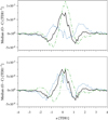 |
Fig. 10 Both the upper and lower panels show the median residuals between the LSF model and selected 1D observations split into three equal percentiles of τ̇ - τ̇0. The solid black line depicts the central third (33-66%), with the lower and upper thirds depicted by the dashed blue and dot-dashed green lines, respectively. In the upper panel, the LSF model is computed using the median value of τ̇ - τ̇0 for the observations, whereas in the lower plot the LSF model is computed using the correct τ̇ - τ̇0 for each observation. |
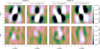 |
Fig. 11 Median residuals of the PSF model for NOGATE observations in a TYPE-01 device (ROW2 AF4; left two columns) and a TYPE-02 device (ROW3 AF9; right two columns). For each device, the left and right columns correspond to observations with μ̇ - μ̇0 < -0.37 and μ̇ - μ̇0 > 0.37 pix s−1, respectively. In the top row the PSF model τ dependence uses a first order spline with no knots. In the bottom row the PSF model τ dependence uses a third order spline with no knots. |
6.2 TDI line dependence in 2D observations
Figure 7 demonstrates the τ dependence in the calibrated PSF model, and its codependence on AC rate and device type due to the corner effect. It is also instructive to inspect the residuals to the 2D NOGATE observations with and without the activation of the τ dependence in the PSF model, in order to demonstrate its impact and justify the choice of a third order dependence on τ in the model configuration. In Fig. 11, we present a series of plots depicting the spatial structure in the residuals between the PSF model and the 2D NOGATE observations, for two different device types and with the observations split by μ̇ - μ̇0. These are derived from recalibrations of the PSF model using two different configurations of the τ dependence. In the top row, the τ dependence uses a first order spline with no knots, which essentially disables it. The residuals to this model show major spatial structure that changes in sign with both the AC rate (due to the inverted relationship between the sample locations and the range of τ over which they were exposed) and the device type (due to the inverted corner effect). In the bottom row, the τ dependence uses a third order spline with no knots, which is the configuration used operationally. In this case the residuals show much less spatial structure that has a much weaker dependence on AC rate and device type. The remaining systematic structure in the residuals is likely dominated by the brighter-fatter effect, with contributions from several other unmodelled effects and known limitations in the model. These are discussed further in Sect. 7.3.
6.3 Calibration of AL and AC shifts
In Sect. 5.1.3, we introduced the AL and AC shifts of the PLSF origin, denoted u0 and v0, and described how they are calibrated by the adoption of a linearised form of the PLSF models and the identities in Eq. (20). The linearised model is an approximation that is only valid over a limited range of u0 and v0, and relies on an accurate mean G0. Here, we present some tests designed to investigate the accuracy of the linearised model and the valid range of u0 and v0.
For selected calibration units, we performed many trial calibrations of the PLSF models, and for each calibration we adjusted the predicted AL and AC locations of the observations by a fixed amount, in order to mimic shifts of the PLSF origin. We then inspect the solution for the g1 and g2 parameters, which should be tightly correlated with the applied adjustments within the valid range of the model. Figure 12 presents the results for the LSF model, for both FOVs in the device in row 4 strip AF5. The upper panel plots the difference between the applied u0 and the recovered g1 , as a function of u0. Note that g1 has dependences on νeff and μ and has been sampled at νeff = 1.43 μm−1 and μ = 1000 pix respectively; this choice is arbitrary since the applied u0 shift has no dependence on these. The divergence from zero for |u0| ≳ 0.2 TDI1 indicates breakdown of the model and the extent of the valid range of u0. For both FOVs g1 - u0 is roughly linear within this region, with g1 /u0 ≈ 1.04 for FOV1 and g1/u0 ≈ 1.01 for FOV2. Ideally we would have g1/u0 = 1; the observed offset from unity is due to differences between the true mean LSF and the G0 function used in the model, which in the DR4 processing is a fixed function for all devices in the same FOV. This is known to be sub-optimal since the LSF for each telescope varies significantly across the focal plane and in time. The lower panel in Fig. 12 indicates a gradual degradation in the LSF solution as a function of the applied shift.
Figure 13 presents the equivalent results for the FOV1 NOGATE PSF calibrations in the same device, now including the AC terms and analysis of the combined shifts. For the PSF, we have the additional complication that the g1 and g2 functions have a dependence on τ (see Table 3), with the shift being defined as the value at the gate fiducial line τF. We find that the valid ranges of u0 and v0 are similar to the LSF case (|u0| ≲ 0.2 TDI1, |v0| ≲ 0.2 pix), and that within this range both g1/u0 and g2/v0 exhibit a similar difference from unity. This is partly due to a sub-optimal G0 function, which for the PSF model is split by FOV and additionally by CCD strip. However, it is also partly due to a slight lack of constraint in the dependence of g1 and g2 on τ, which uses a third order spline for the longer gates. In recent processing (post-DR4), we reduced this by adjusting the configuration of the g1 and g2 functions to always use a first order spline in τ.
Finally, the application of the constraints described in Sect. 5.1.3 ensures that successive iterations between the PLSF calibration and the attitude and geometric instrument calibrations have the effect of driving the shifts u0 and v0 present in the real observations towards zero. For the DR4 processing several such iterations were carried out, and the final shift values were well within the valid range of the model (see Castañeda et al., in prep., Sect. 3.5.5.5).
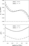 |
Fig. 12 Tests of the calibration of the AL shift using the linearised LSF model. The upper panel depicts the difference between the estimated shift (g1) and the applied value (u0) as a function of u0. The lower panel depicts the goodness-of-fit of the solution as a function of u0, in terms of the χ2 per degree of freedom. |
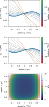 |
Fig. 13 Tests of the calibration of the AL and AC shifts using the linearised PSF model. The upper two panels depict the differences between the estimated AL (g1) and AC (g2) shifts and the applied values (u0 and v0) as a function of u0 and v0 . The lower panel depicts the goodness-of-fit of the solution as a function of u0 and v0, in terms of the χ2 per degree of freedom. |
6.4 Comparison against DR3 PLSF models
Within the overall Gaia data processing, the critical role of the PLSF models is in the determination of the source location (AL, and AC for 2D) and instrumental flux for every observation, quantities collectively referred to as the image parameters. These are estimated using a maximum likelihood algorithm presented in Lindegren (2008), with adaptations for DR4 described in footnote 12 in this paper. The image parameters are the basic observations used in the astrometric and photometric solutions for each source.
We carried out tests to roughly quantify how our improved PLSF models have affected the image parameters relative to those obtained using the DR3 PLSF models described in Paper I. This has been performed by calibrating both our new PLSF models and the equivalent DR3 models to the same set of observations described at the start of this section, and using them both to solve for the image parameters for all the observations. We then compare the estimated source location(s) against the known location for each source, which is obtained from the astrometric solution and provides a suitable ground truth. A similar test of the instrumental flux is unfortunately not possible, due to the inability to invert the photometric calibration (see Sect. 6.4 of Paper I). We therefore focus on the AL and AC source locations in our analysis. Note that for practical reasons we cannot make a direct comparison with the DR3 image parameters for the same set of observations, and must instead approximately recreate the processing that was carried out for DR3 but using the improved DR4 auxiliary calibrations, astrometric solution and PLSF basis components. To imitate the DR3 PLSF, we disabled the analytic model of AL and AC source motion and the dependence on TDI line number, and re-introduced an empirical dependence on AC source motion with the same configuration used in DR3. This allows us to cleanly isolate the effects of the new PLSF model features, while providing only a lower limit on the improvements in the estimated source locations relative to DR3.
Figure 14 presents some selected PSF models from this activity. These clearly demonstrate the limitation of the DR3 model at reproducing the effects of high AC source motion in the CCD gates with longer exposure times. This has been completely overcome in our new work by the transition to an analytic model of this effect. The instabilities evident in the DR3 PSF models shown in Fig. 14 affect the estimation of the source location. This is depicted in Figs. 15 and 16, where we present results for one particular representative CCD. As expected, the change in the estimated source location is greatest for 2D observations and proportional to the gate length. Significant improvements are obtained for ungated 2D observations, corresponding to sources with 11.5 ≲ G ≲ 13, where the distribution of estimated AL and AC source location relative to the ground truth shows a significantly lower scatter and bias. The improvements diminish over gates 12 (11.2 ≲ G ≲ 12.5) and 11 (11 ≲ G ≲ 12), and for gates 10 and shorter (G ≲ 11) the differences are insignificant. Note that the observations in different gates overlap considerably in magnitude, and the ranges given here are approximate. Figure 17 presents the equivalent results for 1D observations in window class 1 (13 ≲ G ≲ 16) in the same CCD; these show no significant change in the AL source location. This is consistent with the minor impact of the AL source motion on the LSF, which is not included in the DR3 model. The main advantage of the updated LSF model is the calibration of AL shifts in the LSF origin, rather than any improvements in the estimated source location.
7 Discussion
In this section, we briefly discuss certain features and limitations of the modelling that have not been explicitly covered so far.
These relate to the processing carried out for DR4 and also to potential improvements for DR5.
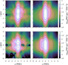 |
Fig. 14 Comparison of the new DR4 (right) and recalibrated DR3 (left) PSF models for a particular calibration unit (NOGATE in ROW5 AF5), recalibrated to selected observations as described in Sect. 6.4. The upper panels correspond to FOV1 and the lower panels to FOV2. The models have been computed for μ̇ - μ̇0 = −1 pix s−1. |
7.1 Expectations for DR4
Relative to EDR3, we expect improvements in the PLSF modelling for all observations due to the introduction of new 1D and 2D basis components, the adjusted configuration of the νeff dependence and improvements to many of the auxiliary instrument calibrations. However, based on the results presented in Sect. 6.4 and elsewhere the largest improvements are expected to be achieved for 2D observations in the longest gates, since these benefit the most from both the drastically improved modelling of the AL and AC smearing effect and the completely new dependence of the PSF shape on τ. This corresponds to sources with (apparent) G magnitude roughly in the 11 to 13 range. Comparing figure 16 in Paper I with Fig. 11 in this paper suggests that the systematic residuals to the model for this subset of the data have reduced in amplitude by at least a factor of ten. The modelling of brighter observations in shorter gates will have improved to a lesser extent. For 1D observations, corresponding to sources with G ≳ 13, we expect more modest improvement, since the AL rate has a relatively minor effect on the LSF compared to other unmodelled dependences described later in this section. Note that this is purely in terms of the residuals to the PLSF models and the measured source locations. Quantitative predictions for the improvements in the derived data products are difficult to make, although we note that in Hernández et al., (in prep.) the 11 to 13 magnitude range clearly shows a greater reduction in the astrometric biases and residuals compared to earlier releases, due at least in part to our improvements in the PSF model.
7.2 Configuration issues
The PLSF models described in this paper have a large number of free parameters that control their joint dependences on the νeff, μ and τ dimensions, each of which has different characteristics. These are fitted across a large number of independent calibration units representing different subsets of the observations that are split broadly by magnitude, detector, window geometry and telescope, and which have varying degrees of sensitivity to different physical effects. This requires a careful choice of the configuration to ensure that the models are able to reproduce the observations across all regions of the parameter space while remaining well constrained. The global configuration presented in Tables 2 and 3 is known to be sub-optimal in several ways.
First, the dependence on μ is fixed across all devices and both FOVs, when in reality the observations exhibit quite complex behaviour. Within certain devices there are localised anomalies in the CCD response that introduce variations in the electronic component of the PLSF that depend on μ. One example is the CCD in row 6 strip AF3, which appears to be thinner over μ = 1100-1300 pix and τ = 2055-4500 pix, i.e. affecting the GATE12 and NOGATE observations which utilise this region of the device. The LSF for both FOVs (and the PSF for NOGATE and GATE12) is significantly narrower in the AL direction over the affected μ range. All the CCDs in row 1 show a rapid and complex variation in the PSF with μ that affects FOV2 much more strongly than FOV1, and is therefore optical in nature. This might be caused by vignetting from the twin periscopes of the Basic Angle Monitor (BAM), which obscure part of the entrance pupil of each telescope, or it could be related to the greater distance of the FOV2 field coordinate origin from row 1 (Bastian 2020). The main impact is on the AC distribution of flux, so the LSF is relatively unaffected. Finally, the CCD in row 5 strip AF2 has a deep charge trap in the serial register around μ = 1258 pix that causes a deficit of flux in all observations at higher μ coordinates. None of these phenomena are well reproduced by the PLSF models due to the lack of flexibility in the μ configuration.
The configuration of the νeff dependence has improved since EDR3, due to the addition of a spline knot and the widening of the calibration range from 1.24-1.72 μm−1 to 1.08-1.9 μm−1, which now encompasses the vast majority of stars. However, there are lingering issues at both the red and blue ends of the range, in the former due to insufficient flexibility in the spline, and in the latter due to limitations in the 2D basis components, which struggle to fit the narrow PSFs of blue sources due to a lack of high spatial frequency components. Both of these issues are limited to the modelling of 2D windows. The lack of high spatial frequency basis components also affects the modelling of 2D observations at low values of |μ̇ - μ̇0|, which have narrow profiles in the AC direction.
As well as extending the basis components to higher spatial frequencies, the 1D bases could be improved by using a different set for each CCD strip, as is currently the case for the 2D bases. For both types, the use of time dependent bases that are updated after each refocus or decontamination event would help reduce time variation in the model performance (see Castañeda et al., in prep, Sect. 3.5.5.5). All of the issues described in this section have already been overcome in the early data processing for DR5, and will not be discussed further.
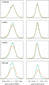 |
Fig. 15 Distribution of the estimated AL (left) and AC (right) source locations relative to their ground truth values, obtained from selected 2D observations in the CCD in row 5 AF5 and corresponding to FOV1 (FOV2 is depicted in Fig. 16). The dot-dashed orange line corresponds to the recalibrated DR3 PSF model and the green line corresponds to the DR4 PSF model. In the top row, observations from CCD gates 410 have been merged; these are the least affected by the updated PSF model. The second, third, and fourth rows correspond to observations from gates 11, 12, and 0, respectively, as indicated in the upper left corner. The plots are normalised to unit area, so the vertical scale is arbitrary and omitted for clarity. |
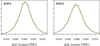 |
Fig. 17 Distribution of the estimated AL source locations relative to their ground truth values, obtained from selected 1D window class 1 observations in the CCD in row 5 AF5 and corresponding to FOV1 (left) and FOV2 (right). The dot-dashed orange line corresponds to the recalibrated DR3 LSF model and the green line corresponds to the DR4 LSF model. The plots are normalised to unit area, so the vertical scale is arbitrary and omitted for clarity. |
7.3 Remaining unmodelled dependences
There are several physical effects present in the data that are completely unaccounted for in the modelling for DR4. We discuss these briefly in this section.
7.3.1 Source AC location for 1D observations
Although the 1D observations do not sample the AC distribution of source flux due to the on-chip binning, the finite extent of the window in the AC direction (12 pixels) means that some (small) fraction of the flux is not captured by the window. This flux loss has an impact on the photometry and since EDR3 is accounted for in the photometric calibration (see Riello et al. 2020, Sect. 4.4). The window placement, which happens on board in real time, is designed to put each source at the centre of the window in the AC direction. However, there is some scatter due to the source sub-pixel location and other factors. These variations in the source AC location in the window have an impact on the shape of the LSF, since a different region of the PSF is being sampled by the window. The shape change can be quite complex since the PSF has some asymmetry in the AC direction.
Figure 18 demonstrates this by plotting the median residuals to the LSF model for a set of 1D observations, with the observations split into three equal percentiles of the source AC location relative to the window centre (the distribution of which differs slightly per CCD and FOV). In the upper panel, we used the nominal DR4 LSF model, and the different percentiles reveal quite strong variations in the data that are unaccounted for in the model. In the lower panel, we recalibrated the LSF model and introduced a new linear dependence on the source AC location. This simple configuration greatly reduces the variation in the residuals. Note that the residuals are net positive in the core due largely to the non-linear effects described in Sect. 7.3.2. Specifically, the solution for the LSF model is weighted towards the brighter, higher signal-to-noise observations which have broader profiles, while the majority of observations are fainter and sharper. There may also be a small bias in the normalisation of the calibrating observations due to the challenges in doing this step accurately, as explained in Sect. 6.4 of Paper I.
This extension to the LSF model was not developed in time for the DR4 processing, but has already been integrated into the software in preparation for the production of DR5. For DR4, the bias in the measured AL image locations arising from this effect has been compensated for in the astrometric solution by the introduction of new calibration terms (see Hernández et al., in prep.).
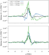 |
Fig. 18 Median residuals between the LSF model and selected 1D observations split into three equal percentiles of source AC location relative to the window centre as indicated in the key, in units of pixels. The solid black line depicts the central third (33-66%), with the lower and upper thirds depicted by the blue and green lines, respectively. In the upper panel, the LSF model has no dependence on the source AC location, whereas in the lower panel this is modelled using a second order spline with no knots (i.e. a simple linear dependence on source AC location; see footnote 16). |
7.3.2 Brighter-fatter effect
The brighter-fatter (BF) effect (Antilogus et al. 2014) is one of several effects present in Gaia’s PLSF that are non-linear in the source flux, and which manifest themselves as a dependence of the PLSF shape on the source magnitude. Note that we prefer the term ‘signal level dependent’ since the effects are actually determined by the photoelectron counts and pixel occupancy, which for Gaia is correlated with the source magnitude only within the range of each CCD gate. Even within a single gate two observations of the same magnitude can have very different pixel occupancy statistics due to the AC smearing and sub-pixel location effects. The BF effect is the tendency for observations of brighter sources (those with higher signal levels) to be systematically wider. It is caused by the deflection of incoming photoelectrons into neighbouring pixels, due to electrostatic repulsion from the charge already present in a pixel. As demonstrated in Fig. 19, the BF effect is very clearly detected in Gaia observations across a wide range in signal level, where it manifests as a systematic trend for observations of brighter sources to have wider profiles in the AL direction. Note that since the LSF model has no existing dependence on signal level it reproduces roughly the average BF present in the calibrating observations, so observations fainter than the average are narrower than the model. Very similar behaviour is seen for 1D and 2D observations, all devices, both FOVs and all CCD gates. It is also observed in the AC direction for 2D observations but at a much lower level, perhaps due to the potential barriers that prevent AC charge transfer, and is dwarfed by serial CTI (Sect. 7.3.3).
No attempt was made to include this effect in the PLSF modelling for DR4. Since the shape distortion is roughly symmetric in AL the impact on the astrometry will be relatively limited. Existing pixel-level models of the BF effect designed for other surveys (e.g. Gruen et al. 2015; Astier & Regnault 2023) have limited applicability to Gaia data due to the use of TDI mode and the complex association between physical pixels and samples in the observations. However, significant work has been done within our group to develop a sample-level model of signal dependent charge redistribution effects in Gaia observations that accounts for BF and potentially other effects, and it remains an ambition to deploy this in the modelling for DR5.
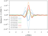 |
Fig. 19 Median residuals between the LSF model and selected 1D observations split into seven equal ranges of source G magnitude. |
7.3.3 Charge transfer inefficiency
Charge transfer inefficiency (CTI) refers to the trapping and release of photoelectrons during the transfer of charge between pixels. It affects Gaia observations in two distinct ways. Parallel CTI (pCTI) occurs in the CCD image section as a source is being observed, and causes a distortion of the image in the AL direction. Serial CTI (sCTI) occurs in the serial register as the image is being read out, and causes a distortion of the image in the AC direction. The various defects that cause charge trapping operate on different timescales, and the two types of CTI are sensitive to different types of defect due to the very different rates at which the charge is clocked in the parallel direction (982.8 μs transfers) versus the serial direction (a complex sequence of 0.1, 10, and 80 μs transfers; Hambly et al. 2018). While sCTI is dominated by defects introduced during manufacture and evolves slowly throughout the mission (Pagani et al. 2026), pCTI becomes significantly stronger over time since it is much more sensitive to the types of defect that are generated in-flight by radiation damage in the space environment (Ahmed et al. 2022, Crowley et al., in prep.). Both types of CTI distort the images of stars by causing a deficit of charge on the leading edge of the profile, i.e. at earlier observation times (pCTI) and closer to the readout node (sCTI), and an excess on the trailing side.
However, pCTI presents a greater risk to the science data due to the resulting systematic bias in the estimated AL image location (Prod’homme et al. 2012; Holl et al. 2012). Hardware level mitigations include the use of periodic charge injections to keep traps filled, and a supplementary buried channel to confine small charge packets to a smaller physical volume of silicon (Seabroke et al. 2013). As shown in Fig. 20, unmitigated pCTI is clearly detected in the data where it manifests as a dependence of the residuals to the LSF model on both the time since the last charge injection and the mission time. The analysis is complicated by the presence of other unmodelled dependences, particularly BF, and the fact that the LSF model itself is calibrated to a non-zero level of pCTI and does not represent an undamaged observation. Considerable work was carried out before launch on the analysis and modelling of pCTI effects given Gaia’s unique observing mode and windowed data (e.g. Prod’homme et al. 2011; Short et al. 2013), with the aim of accounting for the residual effects of unmitigated charge distortion in the data processing via a forwards modelling approach, rather than attempting to reconstruct the undamaged observations (e.g. Massey et al. 2026). Although the image location bias is compensated for in the astrometric processing in a statistical sense via appropriate calibration terms that depend on the charge injection distance, it is our ultimate goal to include a sample-level model of non-linear charge redistribution effects applied on top of the nominal PLSF, in order to account for pCTI on a per-observation basis. However, this has not been integrated into the data processing for DR4, due to a combination of the lower-than-predicted radiation damage levels and the priority given to the modelling of other more significant effects, such as those described in this paper.
Serial CTI affects only the AC distribution of flux within an observation. While it may have a minor impact on the 1D observations by modifying the AC flux loss from the window, it has a large impact on the 2D observations where it manifests as a systematic distortion that depends strongly on both the magnitude and μ coordinate of the observation. This is demonstrated in Fig. 21, which depicts the residuals between the NOGATE PSF model and selected calibration faint star (CFS) observations19, which also use NOGATE and therefore have an identical linear component of the PSF. The NOGATE PSF model is calibrated to observations over the 11 ≲ G ≤ 13 magnitude range, which are significantly brighter than the CFS observations and less affected by sCTI. The CFS observations therfore exhibit quite extreme sCTI symptoms relative to the model, although lower level effects are present in all magnitude ranges. The charge redistribution causes a bias in the estimated AC image location, shifting it to larger μ. This has little impact on the science data since the AC locations have very little dependence on the parallax factor and are not currently included in the astrometric solution for each source. They are, however, useful for both the attitude and geometric instrument calibrations carried out by AGIS. As with both BF and pCTI, while no sample-level modelling of sCTI has been performed for DR4, it may be included in the data processing for future releases as part of our modelling of non-linear charge redistribution effects. Recent work to characterise the trap populations in the serial register, presented in Pagani et al. (2026), will assist in this, although their model cannot be directly applied to science observations for the reasons described therein.
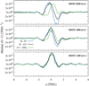 |
Fig. 20 Residuals between the LSF model and selected 1D observations split into three ranges of charge injection distance, as indicated in the key in units of TDI1. The three panels span three different mission times that cover almost the full DR4 time range, with the time indicated in the top right of each panel. |
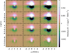 |
Fig. 21 Residuals between the NOGATE PSF model (C) and selected 2D CFS observations (O), split by G magnitude and μ coordinate. The columns from left to right correspond to G = 15-16 mag, 17-18 mag, and 19-20 mag respectively, and the rows from bottom to top correspond to μ = 14-505 pix, 505-997 pix, 997-1488 pix, and 1488-1979 pix, respectively. |
7.4 The GaiaNIR mission
Our work demonstrates the importance of including subtle instrumental effects when producing realistic image models. Since the PSF distortions described in this paper are caused mostly by the spinning and precessing motion of the satellite, rather than for example by the particular detector technology, other missions that use similar observing principles to Gaia will need to consider them. This is critical both during the operational phase for the routine processing of data, but it also plays a vital role during the planning stages for use in deriving accurate performance predictions and error budgeting. Simulations that neglect such effects will necessarily produce optimistic or misleading results. This is particularly true for astrometric surveys due to the complex dependence of the PSF on the AC rate and the strong correlation with the AL parallax factor.
The proposed GaiaNIR mission is currently under consideration for inclusion in the ESA’s Voyage 2050 science programme (Hobbs et al. 2021,?). This spaceborne astrometric survey mission would operate using the same well-established scanning strategy as Gaia and Hipparcos, observing instead at near-infrared (NIR) wavelengths. Due to the lack of NIR-sensitive CCDs capable of operating in TDI mode, alternative detector technologies are being investigated. A promising option are the linear mode avalanche photodiode arrays (LM-APDs; see Rixon et al. 2023). In such a scenario, the TDI mode would be implemented in on-board software by the stacking of many short exposures. This could enable the partial mitigation of the effects of the stellar image motion at the observation level, by shifting the individual exposures prior to stacking, an idea explored in more detail in Høg (2023).
8 Conclusion
We present our improved models of Gaia’s PLSF that have been implemented and deployed in the production of DR4. This will lead to improvements in the astrometry and G-band photometry relative to DR3 that are greater than expected from the increased number of observations alone. Gaia’s unique PSF has taken some time to investigate and model. With the improvements presented in this paper, we now consider the linear part of the PLSF to be well understood. The same model, with certain improvements as discussed, will be deployed in the production of the final catalogue, along with planned additional modelling of several non-linear effects that are at this point still ignored in the PLSF. This work will provide a useful reference both to users of Gaia data and also to future astrometric survey missions that use the same observing principles as Gaia.
Acknowledgements
This work has made use of data from the European Space Agency (ESA) mission Gaia (https://www.cosmos.esa.int/gaia), processed by the Gaia Data Processing and Analysis Consortium (DPAC, https://www.cosmos.esa.int/web/gaia/dpac/consortium). Funding for the DPAC has been provided by national institutions, in particular the institutions participating in the Gaia Multilateral Agreement. The Gaia mission website is: http://www.cosmos.esa.int/gaia. The work described in this paper has been financially supported by the United Kingdom Science and Technology Facilities Council (STFC) and the United Kingdom Space Agency (UKSA) through the following grants: ST/N000595/1, ST/S000976/1, ST/W002493/1, ST/X001601/1, ST/N000595/1, and UKRI9452:APP68395; by the Spanish MICIN/AEI/10.13039/501100011033 and “ERDF - A way of making Europe” by the European Union through grants PID2021-122842OB-C21 and PID2024-157964OB-C21, and the Institute of Cosmos Sciences University of Barcelona (ICCUB, Unidad de Excelencia María de Maeztu) through grant CEX2024-001451-M and the project 2021-SGR-00679 GRC de l’Agència de Gestió d’Ajuts Universitaris i de Recerca (Generalitat de Catalunya); by ESA PRODEX 4000145062; and by the Swedish National Space Board (SNSB/Rymdstyrelsen). Finally, the authors also acknowledge the computer resources from MareNostrum, and the technical expertise and assistance provided by the Red Española de Supercomputación at the Barcelona Supercomputing Center, Centro Nacional de Supercomputación.
References
- Ahmed, S., Hall, D., Crowley, C., et al. 2022, J. Astron. Telesc. Instrum. Syst., 8, 016003 [Google Scholar]
- Anderson, J., & King, I. R. 2000, PASP, 112, 1360 [NASA ADS] [CrossRef] [Google Scholar]
- Antilogus, P., Astier, P., Doherty, P., Guyonnet, A., & Regnault, N. 2014, J. Instrum., 9, C03048 [Google Scholar]
- Astier, P., & Regnault, N. 2023, A&A, 670, A118 [NASA ADS] [CrossRef] [EDP Sciences] [Google Scholar]
- Bastian, U. 2020, GAIA-CA-SP-ARI-BAS-003 https://dms.cosmos.esa.int/COSMOS/doc_fetch.php?id=358698 [Google Scholar]
- Bierman, G. J. 1977, Factorization Methods for Discrete Sequential Estimation (Dover) [Google Scholar]
- Castañeda, J., Hobbs, D., Fabricius, C., et al. 2022, Gaia DR3 documentation Chapter 3: Pre-processing [Google Scholar]
- de Bruijne, J., Lindegren, L., Svensson, O., et al. 2006, GAIA-CA-TN-ESA-JDB-028 https://dms.cosmos.esa.int/COSMOS/doc_fetch.php?id=2694426 [Google Scholar]
- Fabricius, C., Bastian, U., Portell, J., et al. 2016, A&A, 595, A3 [NASA ADS] [CrossRef] [EDP Sciences] [Google Scholar]
- Gaia Collaboration (Brown, A. G. A., et al.) 2016a, A&A, 595, A2 [NASA ADS] [CrossRef] [EDP Sciences] [Google Scholar]
- Gaia Collaboration (Prusti, T., et al.) 2016b, A&A, 595, A1 [NASA ADS] [CrossRef] [EDP Sciences] [Google Scholar]
- Gaia Collaboration (Brown, A. G. A., et al.) 2018, A&A, 616, A1 [NASA ADS] [CrossRef] [EDP Sciences] [Google Scholar]
- Gaia Collaboration (Brown, A. G. A., et al.) 2021, A&A, 649, A1 [NASA ADS] [CrossRef] [EDP Sciences] [Google Scholar]
- Gaia Collaboration (Vallenari, A., et al.) 2023, A&A, 674, A1 [NASA ADS] [CrossRef] [EDP Sciences] [Google Scholar]
- Green, D. A. 2011, Bull. Astron. Soc. India, 39, 289 [Google Scholar]
- Gruen, D., Bernstein, G. M., Jarvis, M., et al. 2015, J. Instrum., 10, C05032 [Google Scholar]
- Gunn, J. E., Carr, M., Rockosi, C., et al. 1998, AJ, 116, 3040 [NASA ADS] [CrossRef] [Google Scholar]
- Hambly, N. C., Cropper, M., Boudreault, S., et al. 2018, A&A, 616, A15 [NASA ADS] [CrossRef] [EDP Sciences] [Google Scholar]
- Hobbs, D., Brown, A., Høg, E., et al. 2021, Exp. Astron., 51, 783 [NASA ADS] [CrossRef] [Google Scholar]
- Hobbs, D., Lindegren, L., Bastian, U., et al. 2022, Gaia DR3 documentation Chapter 4: Astrometric data [Google Scholar]
- Høg, E. 2023, arXiv e-prints [arXiv:2312.00488] [Google Scholar]
- Holl, B., Prod’homme, T., Lindegren, L., & Brown, A. G. A. 2012, MNRAS, 422, 2786 [Google Scholar]
- Lindegren, L. 2008, GAIA-C3-TN-LU-LL-078 https://dms.cosmos.esa.int/COSMOS/doc_fetch.php?id=2861864 [Google Scholar]
- Lindegren, L. 2009, GAIA-C3-TN-LU-LL-084 https://dms.cosmos.esa.int/COSMOS/doc_fetch.php?id=2915742 [Google Scholar]
- Lindegren, L. 2010, GAIA-C3-TN-LU-LL-090 https://dms.cosmos.esa.int/COSMOS/doc_fetch.php?id=3049411 [Google Scholar]
- Lindegren, L. 2025a, GAIA-C3-TN-LU-LL-134 https://dms.cosmos.esa.int/COSMOS/doc_fetch.php?id=1736895 [Google Scholar]
- Lindegren, L. 2025b, GAIA-CU3-TN-LU-LL-056 https://dms.cosmos.esa.int/COSMOS/doc_fetch.php?id=1729223 [Google Scholar]
- Lindegren, L., Lammers, U., Hobbs, D., et al. 2012, A&A, 538, A78 [NASA ADS] [CrossRef] [EDP Sciences] [Google Scholar]
- Lindegren, L., Klioner, S. A., Hernández, J., et al. 2021, A&A, 649, A2 [EDP Sciences] [Google Scholar]
- Massey, R., Kegerreis, J. A., Barrios, J. P. L. G., et al. 2026, MNRAS, 546, staf2186 [Google Scholar]
- McEwen, A. S., Eliason, E. M., Bergstrom, J. W., et al. 2007, J. Geophys. Res.: Planets, 112 [Google Scholar]
- Pagani, C., Hambly, N., Davidson, M., et al. 2026, A&A, 707, A218 [NASA ADS] [CrossRef] [EDP Sciences] [Google Scholar]
- Prod’homme, T., Brown, A. G. A., Lindegren, L., Short, A. D. T., & Brown, S. W. 2011, MNRAS, 414, 2215 [Google Scholar]
- Prod’homme, T., Holl, B., Lindegren, L., & Brown, A. G. A. 2012, MNRAS, 419, 2995 [Google Scholar]
- Refregier, A. 2003, MNRAS, 338, 35 [Google Scholar]
- Riello, M., De Angeli, F., Evans, D. W., et al. 2020, A&A, 649, A3 [Google Scholar]
- Rixon, G., Walton, N., Busso, G., et al. 2023, Detector options for GaiaNIR [Google Scholar]
- Robinson, M. S., Brylow, S. M., Tschimmel, M., et al. 2010, Space Sci. Rev., 150, 81 [CrossRef] [Google Scholar]
- Rowell, N., Davidson, M., Lindegren, L., et al. 2021, A&A, 649, A11 [EDP Sciences] [Google Scholar]
- Seabroke, G. M., Prod’homme, T., Murray, N. J., et al. 2013, MNRAS, 430, 3155 [Google Scholar]
- Short, A., Crowley, C., de Bruijne, J. H. J., & Prod’homme, T. 2013, MNRAS, 430, 3078 [Google Scholar]
- van Leeuwen, F. 2007, Astrophysics and Space Science Library, 350, Hipparcos, the New Reduction of the Raw Data (Springer Dordrecht) [Google Scholar]
Additional windows (referred to as ‘virtual objects’) are assigned according to a fixed pattern, for use in several auxiliary calibrations. See Gaia Collaboration (2016b) Sect. 3.3.5 for more details of the windowing.
Sometimes also referred to as the ‘preceding’ and ‘following’ field of view (PFoV and FFoV) in other Gaia publications.
There are 14 prescan pixels lying at μ = 0 to 13. These play no role in this paper.
They are in fact expected to be different, due at least to the use of different magnitude ranges for the calibrating observations (resulting in different signal-level-dependent effects), and to the varying AC source location in the window, a dependence that is not yet incorporated in the LSF model (see Sect. 7.3.1).
Although the corner effect dominates, there are other isolated anomalies in certain devices, and a pair of devices (AF5 and AF8 in ROW2) that both have a low outlying AL FWHM due to being unusually thin. This is visible in figure 12 in Paper I. What was not recognised at the time is that they are twin devices manufactured from the same wafer (see Appendix C).
A sample with larger u reaches the serial register later.
The veff value for each source is computed by PhotPipe from the mean BP and RP spectra, and is by necessity taken from the previous data release, in this case DR3. For DR4 processing, the veff value actually used in the PLSF calibration is a weighted combination of the measured value and a prior, as explained in Hernández et al., (in prep.). See also de Bruijne et al. (2006).
When processing Gaia observations, for both PLSF calibration and window modelling purposes, we use the μ value of the window centre rather than that of the source contained within it, since this may not be known in advance. This may differ from the μ of the source by up to a few pixels, which has no significant effect on the PLSF.
In Paper I the symbol H was used to denote both f and h; in the present paper these functions need to be distinguished.
An alternative value of τmin = 6 would give a ∆τ consistent with the exposure time, though this would still be an approximation for the integral over τ. The particular choice makes no significant difference.
Specifically, when |(τ̇ - τ̇0) texp| or |(μ̇ - μ̇0) texp| are below a threshold, chosen to be 10−5 pixels.
In previous data releases this procedure was called simply Image Parameter Determination (IPD). The processing for DR4 includes a new step of on-ground source detection in order to improve the image parameters of sources in situations where one or more secondary sources appear in the same window, which risks biasing the image parameters of the target source if unaccounted for in the model. This is now referred to as Astrometric Detection and Image Parameter Determination, with the acronym DIPD.
Note that Lindegren (2025a) omits the dependence on τ in Sect. 4.2 since it was written before the τ dependence was recognised; this does not affect the conclusions.
Technically, 1D observations can use a shorter gate (or indeed, multiple gates) if they coincide with the transit of a brighter star which has a higher priority in the gate selection. These accidentally gated observations are not used in the LSF calibration.
The predicted location is obtained using the source astrometry, satellite attitude and geometric instrument calibrations.
By convention a spline of order N has polynomial segments of degree N - 1, such that a spline of order 2 has linear segments and so forth.
As described in Castañeda et al., (in prep., Sect. 3.2.4.1) the νeff value used throughout the data processing is a weighted combination of the νeff computed by PhotPipe, from the mean XP spectrum, and a default value of 1.43 μm−1 that serves as a prior. Extreme unphysical values of νeff are replaced entirely with the default. This is applied upstream of the PLSF.
Corresponding roughly to 1-4 November 2016; a tool for transformation between OBMT and other time systems is available at https://gaia.esac.esa.int/decoder/obmtDecoder.jsp
A small, random fraction of faint (G > 13) observations that would normally be assigned 1D windows are instead assigned 2D windows, for the purposes of calibrating various instrumental effects at the faint end, including sCTI. These are known as calibration faint stars.
Appendix A Along-scan pixel scale estimation
As explained in Sect. 2 the AL angular pixel scale pτ is required in order to convert the stellar image drift rate from angular units (mas s−1) to spatial units (pix s−1), for input to the PLSF modelling. During development of the PSF model described in this paper we found that the nominal value of the AL angular pixel scale (a single, fixed value of pτ = 58.933 mas pix−1 ) is not sufficiently accurate for this. In reality, the pixel scale varies between the two telescopes due to differences in the focal length. It also varies in time due to evolution in the focus, and across the focal plane with several possible causes, such as optical aberrations, variations in pixel pitch and CCD vertical mounting error. As such, a calibrated value of pτ is required in order to account for these effects.
While the geometric part of the AGIS instrument model (see Lindegren et al. 2012, Sect. 3.4) includes no explicit calibration of pτ, we found that it can be estimated to sufficient accuracy by using the calibrated angular positions of the CCD fiducial lines. Specifically, the calibrated η field angle for a particular CCD gate provides an estimate of the angular position of the gate fiducial line, which itself lies at a fixed position in the along scan direction on the CCD (e.g. see Table 1). By comparing the η value for several different CCD gates within the same device, we can estimate the dependence of η on the TDI line number, the gradient of which corresponds to pτ, i.e. pτ = ∂η(τ)/∂τ.
This is depicted in Fig. A.1, where in the upper panel we plot η against TDI line number for the five longest CCD gates. The positions of the gate fiducial lines are indicated with the vertical grey lines. Long gates provide better constraint as the fiducial lines are further apart, so gates shorter than 9 are not used. The purple line is a linear fit to the points, with the lower panel depicting the residuals. The (constant) gradient of the fitted line gives the calibrated value of pτ , which in this example is 58.927 mas pix−1. In principle a higher order fit could be performed, which would allow the estimated pixel scale to vary in the AL direction. However, a constant value was found to be sufficient, which is fortunate since a significant dependence of pτ on TDI line number would greatly complicate the PSF modelling. Finally, this algorithm cannot be applied to SM devices because only GATE12 is present. Instead, we use the equivalent AF1 value and apply a small correction factor that was determined by a separate optimisation procedure. In Fig. A.2 we depict the variation in AL pixel scale across the focal plane, for FOV1 at revolution 4500. The variation is generally quite smooth. In Fig. A.3 we depict the time evolution in the AL pixel scale for one particular calibration. The discontinuities are associated with thermal decontaminations, refocuses and other major mission events.
Appendix B Native AC rate estimation
The native AC rate μ̇0 (see Sect. 2) is the AC rate at which the AC smearing is minimal. It is offset from zero due to a combination of optical effects and small orientation errors in the placement of the CCDs in the focal plane. The value of μ̇0 is required in order to convert the source AC motion to the corresponding AC smearing width, and it therefore needs to be measured and incorporated into the calibration pipeline.
Fortunately, μ̇0 can be measured directly from the observations in a relatively simple manner, using the principle that sources moving at μ̇0 are minimally smeared AC. We first select a large number of ungated 2D observations, which are then debiased, background-subtracted, normalised, and finally marginalised to form the 1D LSF in the AC direction. These are aligned according to the predicted AC location of the source, and binned into narrow ranges of AC rate. Within each bin we estimate the AC full-width-half-maximum (FWHM) of the observations, by fitting a polynomial to the samples then finding the maximum and the two adjacent half-maximum locations. This is performed independently for each FOV and CCD combination; in Fig. B.1 we present two plots depicting the polynomial fits for two different AC rate bins in FOV1 ROW3 AF5. The three vertical lines indicate the maximum and half-maximum locations from which the AC FWHM is derived, with the resulting values indicated in the figures.
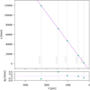 |
Fig. A.1 Estimation of the FOV1 AL pixel scale in device ROW1 AF7, at AC coordinate 1000 and at revolution 4500. The vertical grey lines indicate the positions of the fiducial lines for the 5 longest CCD gates, which are the ones used operationally to estimate the pixel scale. |
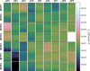 |
Fig. A.2 Variation in AL pixel scale across the focal plane as determined by the algorithm described in this section, for FOV1 at revolution 4500. |
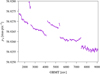 |
Fig. A.3 Evolution in AL pixel scale over most of the DR4 time range, for one particular calibration (FOV1 ROW1 AF7 at AC coordinate 1000). |
This procedure results in a set of discrete samples of the AC FWHM as a function of AC rate, with observations at high positive and negative AC rate having the largest AC FWHM and the minimum falling close to zero. The precise location of the minimum gives the value for μ̇0; this needs to be estimated to an accuracy finer than the bin size in AC rate, so we must fit an interpolating function to the samples. Empirically, the resulting profile has a roughly hyperbolic form, and we found that it can be well modelled in all devices and FOVs by the pseudo-hyperbolic function

where A, B, C, D, E, F, and G are free parameters that are fitted using the Levenberg-Marquardt algorithm. The native AC rate corresponds to the translation from the origin, which is given by the parameter C. In Fig. B.2 we depict this fitting procedure for the two FOVs in a single CCD (ROW3 AF5).
This procedure estimates an independent, constant value of μ0 for each FOV and CCD. Within the same device the two FOVs have similar values of μ0 due partly to the common CCD rotation error and partly to similar projection effects in the same region of the focal plane. This is evident in Fig. B.3, which shows the correlation of μ̇0 between FOV1 and FOV2, for all AF devices. SM devices are excluded because each is used by only one of the two FOVs. Note that the use of a single, constant value of μ̇0 for each FOV and CCD ignores any possible time dependence or spatial variation within each device. We checked for time dependence in μ̇0 and found it to be negligible. Spatial variation in the AC direction within each device is likely to be more significant, albeit small, and in future data processing we may allow μ̇0 to additionally depend on AC position in the CCD.
Appendix C CCD device types and twins
In Fig. C.1 we present the CCD type information for all SM and AF devices, where the type refers to whether the CCD was manufactured from the left half (TYPE-01) or the right half (TYPE-02) of the circular silicon wafer. As explained in Sect. 3.2, the type has an impact on spatial variations in the CCD response and the behaviour of different gates, due to the corner effect. In Table C.1 we list all twin CCDs in SM and AF, where a ‘twin’ refers to two devices that have been manufactured from the same wafer. Twin devices can sometimes exhibit similar behaviour. Most devices are not twinned with another.
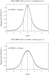 |
Fig. B.1 Example estimation of the AC FWHM as a function of AC rate, for one particular FOV (FOV1) and CCD (ROW3 AF5). The upper and lower panels correspond to ungated 2D observations in the AC rate ranges 0.175-0.200 and 0.6000.625 pix s−1, respectively. The grey points are samples from the marginalised and normalised AC LSFs of a large number of observations, aligned according to the AC location of the source. The black curve is a polynomial fit to the samples, with the vertical lines indicating the maximum and half-maximum locations from which the AC FWHM (quoted in the figures) is derived. |
Appendix D Numerical integration by Gauss-Legendre quadrature
The PSF model presented in Eq. 12 and its associated first derivatives include three integrals over τ that must be evaluated numerically. For convenience, the integrands will be denoted
P(τ), Q(τ) and R(τ) where
 (D.1)
(D.1)
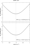 |
Fig. B.2 Example estimation of the native AC rate μ̇0 for FOV1 (upper panel) and FOV2 (lower) in the same device (ROW3 AF5). The value of μ̇0 coincides with the AC rate for which the AC FWHM is minimised, as determined by fitting an appropriate pseudo-hyperbolic function (grey line) through the data (black dots). The vertical dashed lines indicate the minimum of the interpolating function, which provides the estimate of μ̇0. |
Twin CCDs among all SM and AF devices.
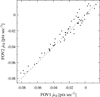 |
Fig. B.3 Native AC rate μ̇0 in FOV1 and FOV2 for all AF devices. |
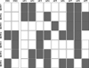 |
Fig. C.1 Layout of the SM and AF part of the focal plane and the distribution of CCD types among the devices; TYPE-01 devices are indicated in grey, and TYPE-02 devices are indicated in white. |
A few selected examples of P(τ), Q(τ), and R(τ) are depicted in Fig. D.1. Many different numerical integration methods exist, and while the accuracy of any method generally depends on the kind of functions that are being integrated, this must also be balanced against our implementation requirements of low execution time and memory footprint. We tested both Romberg’s method and Gauss-Legendre quadrature, and found the latter to have significantly lower numerical integration error for the same number of function evaluations. In Fig. D.2 we present the relative error in the Gauss-Legendre algorithm as a function of the number of steps used, for each of the functions in Fig. D.1 We selected the K = 9 step algorithm as an appropriate balance of the integration error and number of function evaluations that optimises the available execution time. The corresponding function evaluation points τk and associated weight factors wk for k = 0 to K - 1 are listed in Table D.1; these are the values used in Eq. 13 and throughout this work.
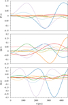 |
Fig. D.1 Selected examples of the P(τ), Q(τ), and R(τ) functions from Eq. D.1 that must be integrated numerically. These have been generated for a range of values of the u, v, η̇, ζ̇, i, and j parameters encountered in routine processing, and correspond to NOGATE for which the τ coordinate spans 1 to 4500. |
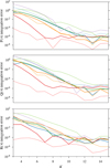 |
Fig. D.2 Relative error in the Gauss-Legendre numerical integration of the functions in Fig. D.1 for different numbers of steps K. The relative integration error is defined as |(IK- I200)/I200|, where IK is the result using K steps. |
Gauss-Legendre quadrature configuration.
All Tables
All Figures
|
Fig. 1 Schematic diagram of one of Gaia’s CCDs, as seen from the illuminated side and showing various features relevant to the PSF modelling. The (τ,μ) coordinates represent positions within the pixel grid. The images of stars move from left to right during integration, with the serial register lying on the right. The main AL and AC directions and their relation to the field angles η and ζ are indicated at the top left. Fiducial lines and barriers for the five longest gates are indicated; NOGATE has no corresponding barrier and uses the entire AL range. |
| In the text | |
|
Fig. 2 Example window geometry and sampling strategy for a simulated G ≈ 13 source in window class 0 (WC0; upper left) and WC1 (upper right). These particular configurations apply to sources with onboard-estimated G < 13 (WC0) and 13 < G < 16 (WC1), in CCD strips AF2-9. Faint grey lines mark the boundaries between individual samples. The red boxes mark the extent of the window region, with the internal black lines indicating the binning of individual samples. The lower panels depict the resulting downlinked 2D (left) and 1D (right) observations. |
| In the text | |
|
Fig. 3 Example of the observed AL (upper) and AC (lower) stellar image drift rates relative to the transferring charge over a two-revolution (12 hour) period, for both FOVs and measured at the centre of a CCD in row 1. |
| In the text | |
|
Fig. 4 Effects of AL and AC source motion on the PSF. These plots depict the integrated effective PSF for three different regimes of τ̇ and μ̇. The u and v coordinates are relative to the PSF origin, as explained at the start of Sect. 4.1. These plots have been generated using the calibrated PSF model presented later in this paper, and correspond to the FOV1 PSF for NOGATE observations in the ROW2 AF4 device. In the left panel τ̇ = τ̇0 and μ̇ = μ̇0 such that the stellar image motion is perfectly matched to the charge transfer and no smearing occurs in either dimension. In both the centre and right panels τ̇ - τ̇0 = 0.226 pix s−1, such that the stellar image lags one pixel behind the charge in the AL direction during the 4.42 second exposure. In the centre and right panels μ̇ - μ̇0 = 0.974 and −0.974 pix s−1 respectively, such that the stellar image moves ±4.3 pixels in the AC direction, orthogonally to the charge transfer. Note that the τ̇ value is about 20 times larger than what is routinely observed in the real data, in order to make the impact on the PSF more obvious for the plots. Throughout this paper we make use of the cubehelix colour scheme introduced in Green (2011). |
| In the text | |
|
Fig. 5 Illustrative example of (artificial) flatfield images for a pair of CCDs manufactured from the same circular silicon wafer. This figure approximately reproduces the effect seen in industrial pre-launch flatfield data from Gaia’s CCDs at 900 nm, and which cannot be published. The CCD on the left is of TYPE-01 and the CCD on the right is of TYPE-02. |
| In the text | |
|
Fig. 6 Effects of AL variations in the CCD response on the PSF, and the dependence on CCD gate and device type. The AL FWHM of the integrated effective PSF is plotted as a function of CCD gate, for two devices of TYPE-01 (ROW2 AF4, dot-dashed line) and TYPE-02 (ROW3 AF9, solid line). Each CCD gate spans a range in τ, with the points plotted at the fiducial line positions. The solid squares correspond to FOV1 and the open circles to FOV2. These figures have been generated using the calibrated PSF model rather than directly from the observations. |
| In the text | |
|
Fig. 7 Effects of AL variations in the CCD response on the PSF, and the dependence on source motion. Each plot shows the difference between two integrated effective PSFs for τ̇ = τ̇0 and μ̇ - μ̇0 = ±1.0 pix s−1, such that the PSFs are smeared exclusively in the AC direction. The PSFs are for NOGATE, so the entire τ range of the CCD is covered. Due to the AC motion, the lower half of each plot shows the approximate difference between the instantaneous effective PSF at high τ minus the instantaneous effective PSF at low τ, and vice-versa in the upper half. The lower panel is a TYPE-01 device (ROW2 AF4) and the upper panel is a TYPE-02 device (ROW3 AF9). |
| In the text | |
|
Fig. 8 Reproduction of the effects of AL and AC source motion in the PSF model. The upper two panels show two model PSFs that are identical apart from the configured AL and AC source motion: in both cases τ̇ - τ̇0 = −0.045 pix s−1 while μ̇ - μ̇0 = −0.975 (left) and 0.975 (right) pix s−1. The lower left panel shows the difference between the two, which is dominated by the reversed sign of the shearing effect due to the change in sign of the AC rate. The lower right panel depicts the equivalent effect seen directly in the data, and is produced by stacking many observations at μ̇ − μ̇0 > 0.975 and μ̇ - μ̇0 < -0.975 pix s−1 and plotting the difference. |
| In the text | |
|
Fig. 9 Reproduction of the effect of AL source motion in the LSF model. The upper panel shows four model LSFs for four different values of τ̇ - τ̇0 ranging from 0.0 to 0.06 pix s−1. The lower panel shows the differences relative to the LSF for τ̇ - τ̇0 = 0.0 pix s−1. |
| In the text | |
|
Fig. 10 Both the upper and lower panels show the median residuals between the LSF model and selected 1D observations split into three equal percentiles of τ̇ - τ̇0. The solid black line depicts the central third (33-66%), with the lower and upper thirds depicted by the dashed blue and dot-dashed green lines, respectively. In the upper panel, the LSF model is computed using the median value of τ̇ - τ̇0 for the observations, whereas in the lower plot the LSF model is computed using the correct τ̇ - τ̇0 for each observation. |
| In the text | |
|
Fig. 11 Median residuals of the PSF model for NOGATE observations in a TYPE-01 device (ROW2 AF4; left two columns) and a TYPE-02 device (ROW3 AF9; right two columns). For each device, the left and right columns correspond to observations with μ̇ - μ̇0 < -0.37 and μ̇ - μ̇0 > 0.37 pix s−1, respectively. In the top row the PSF model τ dependence uses a first order spline with no knots. In the bottom row the PSF model τ dependence uses a third order spline with no knots. |
| In the text | |
|
Fig. 12 Tests of the calibration of the AL shift using the linearised LSF model. The upper panel depicts the difference between the estimated shift (g1) and the applied value (u0) as a function of u0. The lower panel depicts the goodness-of-fit of the solution as a function of u0, in terms of the χ2 per degree of freedom. |
| In the text | |
|
Fig. 13 Tests of the calibration of the AL and AC shifts using the linearised PSF model. The upper two panels depict the differences between the estimated AL (g1) and AC (g2) shifts and the applied values (u0 and v0) as a function of u0 and v0 . The lower panel depicts the goodness-of-fit of the solution as a function of u0 and v0, in terms of the χ2 per degree of freedom. |
| In the text | |
|
Fig. 14 Comparison of the new DR4 (right) and recalibrated DR3 (left) PSF models for a particular calibration unit (NOGATE in ROW5 AF5), recalibrated to selected observations as described in Sect. 6.4. The upper panels correspond to FOV1 and the lower panels to FOV2. The models have been computed for μ̇ - μ̇0 = −1 pix s−1. |
| In the text | |
|
Fig. 15 Distribution of the estimated AL (left) and AC (right) source locations relative to their ground truth values, obtained from selected 2D observations in the CCD in row 5 AF5 and corresponding to FOV1 (FOV2 is depicted in Fig. 16). The dot-dashed orange line corresponds to the recalibrated DR3 PSF model and the green line corresponds to the DR4 PSF model. In the top row, observations from CCD gates 410 have been merged; these are the least affected by the updated PSF model. The second, third, and fourth rows correspond to observations from gates 11, 12, and 0, respectively, as indicated in the upper left corner. The plots are normalised to unit area, so the vertical scale is arbitrary and omitted for clarity. |
| In the text | |
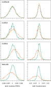 |
Fig. 16 Equivalent to Fig. 15 for FOV2. |
| In the text | |
|
Fig. 17 Distribution of the estimated AL source locations relative to their ground truth values, obtained from selected 1D window class 1 observations in the CCD in row 5 AF5 and corresponding to FOV1 (left) and FOV2 (right). The dot-dashed orange line corresponds to the recalibrated DR3 LSF model and the green line corresponds to the DR4 LSF model. The plots are normalised to unit area, so the vertical scale is arbitrary and omitted for clarity. |
| In the text | |
|
Fig. 18 Median residuals between the LSF model and selected 1D observations split into three equal percentiles of source AC location relative to the window centre as indicated in the key, in units of pixels. The solid black line depicts the central third (33-66%), with the lower and upper thirds depicted by the blue and green lines, respectively. In the upper panel, the LSF model has no dependence on the source AC location, whereas in the lower panel this is modelled using a second order spline with no knots (i.e. a simple linear dependence on source AC location; see footnote 16). |
| In the text | |
|
Fig. 19 Median residuals between the LSF model and selected 1D observations split into seven equal ranges of source G magnitude. |
| In the text | |
|
Fig. 20 Residuals between the LSF model and selected 1D observations split into three ranges of charge injection distance, as indicated in the key in units of TDI1. The three panels span three different mission times that cover almost the full DR4 time range, with the time indicated in the top right of each panel. |
| In the text | |
|
Fig. 21 Residuals between the NOGATE PSF model (C) and selected 2D CFS observations (O), split by G magnitude and μ coordinate. The columns from left to right correspond to G = 15-16 mag, 17-18 mag, and 19-20 mag respectively, and the rows from bottom to top correspond to μ = 14-505 pix, 505-997 pix, 997-1488 pix, and 1488-1979 pix, respectively. |
| In the text | |
|
Fig. A.1 Estimation of the FOV1 AL pixel scale in device ROW1 AF7, at AC coordinate 1000 and at revolution 4500. The vertical grey lines indicate the positions of the fiducial lines for the 5 longest CCD gates, which are the ones used operationally to estimate the pixel scale. |
| In the text | |
|
Fig. A.2 Variation in AL pixel scale across the focal plane as determined by the algorithm described in this section, for FOV1 at revolution 4500. |
| In the text | |
|
Fig. A.3 Evolution in AL pixel scale over most of the DR4 time range, for one particular calibration (FOV1 ROW1 AF7 at AC coordinate 1000). |
| In the text | |
|
Fig. B.1 Example estimation of the AC FWHM as a function of AC rate, for one particular FOV (FOV1) and CCD (ROW3 AF5). The upper and lower panels correspond to ungated 2D observations in the AC rate ranges 0.175-0.200 and 0.6000.625 pix s−1, respectively. The grey points are samples from the marginalised and normalised AC LSFs of a large number of observations, aligned according to the AC location of the source. The black curve is a polynomial fit to the samples, with the vertical lines indicating the maximum and half-maximum locations from which the AC FWHM (quoted in the figures) is derived. |
| In the text | |
|
Fig. B.2 Example estimation of the native AC rate μ̇0 for FOV1 (upper panel) and FOV2 (lower) in the same device (ROW3 AF5). The value of μ̇0 coincides with the AC rate for which the AC FWHM is minimised, as determined by fitting an appropriate pseudo-hyperbolic function (grey line) through the data (black dots). The vertical dashed lines indicate the minimum of the interpolating function, which provides the estimate of μ̇0. |
| In the text | |
|
Fig. B.3 Native AC rate μ̇0 in FOV1 and FOV2 for all AF devices. |
| In the text | |
|
Fig. C.1 Layout of the SM and AF part of the focal plane and the distribution of CCD types among the devices; TYPE-01 devices are indicated in grey, and TYPE-02 devices are indicated in white. |
| In the text | |
|
Fig. D.1 Selected examples of the P(τ), Q(τ), and R(τ) functions from Eq. D.1 that must be integrated numerically. These have been generated for a range of values of the u, v, η̇, ζ̇, i, and j parameters encountered in routine processing, and correspond to NOGATE for which the τ coordinate spans 1 to 4500. |
| In the text | |
|
Fig. D.2 Relative error in the Gauss-Legendre numerical integration of the functions in Fig. D.1 for different numbers of steps K. The relative integration error is defined as |(IK- I200)/I200|, where IK is the result using K steps. |
| In the text | |
Current usage metrics show cumulative count of Article Views (full-text article views including HTML views, PDF and ePub downloads, according to the available data) and Abstracts Views on Vision4Press platform.
Data correspond to usage on the plateform after 2015. The current usage metrics is available 48-96 hours after online publication and is updated daily on week days.
Initial download of the metrics may take a while.