| Issue |
A&A
Volume 708, April 2026
|
|
|---|---|---|
| Article Number | A32 | |
| Number of page(s) | 9 | |
| Section | Interstellar and circumstellar matter | |
| DOI | https://doi.org/10.1051/0004-6361/202659335 | |
| Published online | 25 March 2026 | |
Bonnor-Ebert sphere collapse in filamentary structures
1
Universitäts-Sternwarte, Ludwig-Maximilians-Universität München,
Scheinerstr. 1,
81679
Munich,
Germany
2
Excellence Cluster ORIGINS,
Boltzmannstrasse 2,
85748
Garching,
Germany
3
Max-Planck Institute for Extraterrestrial Physics,
Giessenbachstr. 1,
85748
Garching,
Germany
★ Corresponding author: This email address is being protected from spambots. You need JavaScript enabled to view it.
Received:
5
February
2026
Accepted:
19
February
2026
Abstract
Context. Star formation within filaments may arise due to the growth of cores according to linear perturbation theory. This implies a minimum core separation, as shorter modes would not be able to grow. While many observations agree with core separations by theoretical predictions, some observations also show star forming cores which lie closer together than the minimum wavelength given by perturbation theory.
Aims. We explore whether non-linear effects during the late stages of core growth can explain the discrepancy between theory and observations.
Methods. We perform 3D hydrodynamical simulations with the RAMSES code to follow the evolution of initial perturbations within filaments and compare the measured growth rates to expectations from theoretical models.
Results. Non-linear evolution sets in as soon as the core mass reaches a value where the gravitational potential is no longer dominated by the cylindrical potential of the filament but by the spherical potential of the Bonnor-Ebert sphere. Consequently, core collapse is not triggered by the loss of hydrostatic stability of the filament but by the loss of hydrostatic stability of the Bonnor-Ebert sphere. As the core is embedded in the filament, the maximum core mass is given by the pressure within the filament, resulting in a constant line-mass threshold for core collapse.
Conclusions. As core collapse is triggered as soon as overdensities reach a certain line-mass, cores which form as large line-mass perturbations during filament formation can go into direct collapse even if their separation is closer than predicted by linear perturbation theory. Therefore, our result can explain the discrepancy between theory and observations.
Key words: stars: formation / ISM: kinematics and dynamics / ISM: structure
© The Authors 2026
 Open Access article, published by EDP Sciences, under the terms of the Creative Commons Attribution License (https://creativecommons.org/licenses/by/4.0), which permits unrestricted use, distribution, and reproduction in any medium, provided the original work is properly cited.
This article is published in open access under the Subscribe to Open model. This email address is being protected from spambots. You need JavaScript enabled to view it. to support open access publication.
1 Introduction
Star formation is a multi-scale process. Relatively diffuse gas within molecular clouds of sizes of a few tens of parsecs is gravitationally compressed to high densities within star-forming cores with sizes of a few tenths of parsecs. However, this gravitational cascade has an intermediate step forming filamentary structures that contain regularly spaced cores already seen in early extinction and infrared observations (Schneider & Elmegreen 1979). The importance of filaments as an initial condition for core formation was emphasised by the high dynamic range dust observations of the Herschel Space Telescope (André et al. 2010; Molinari et al. 2010). It revealed a high degree of filamentary organisation in nearby molecular clouds and established a clear connection between cores and filaments (Könyves et al. 2015). Newer continuum and line observations have refined this picture and the filamentary structure is now well established at all scales in the interstellar medium of the Milky Way (see Hacar et al. 2023 for a recent review).
A fundamental question for the formation of stars has been the influence of filaments on the core collapse process. In principle, filaments are able to affect the distribution and masses of stars by providing the gravitational environment and mass reservoir for star-forming cores. The idea of filament fragmentation into quasi-regular spaced cores that eventually collapse and form stars has been predicted by theoretical models (see Sect. 2.2) with a minimum wavelength required for perturbations to grow, called the critical wavelength, and a fastest growing mode of about twice the minimum wavelength, also called the dominant wavelength. In principle, cores can form on any wavelength during filament formation. However, non-growing modes are not expected to become massive enough to eventually collapse. Although the comparison of observations and theory is not straightforward and there are issues concerning low number statistics, many studies do find separations that agree with the fastest growing mode, with or without considering a non-isothermal contribution (Jackson et al. 2010; Miettinen 2012; Busquet et al. 2013; Lu et al. 2014; Wang et al. 2014; Beuther et al. 2015; Contreras et al. 2016; Kainulainen et al. 2016; Liu et al. 2018; Lu et al. 2018; Cao et al. 2022; He et al. 2023; Chung et al. 2024; Yang et al. 2024). Nevertheless, there are also studies that show closer separations, either twice as short, as would be the case for the critical wavelength, or even closer by a factor of three or more, as would be the case for the 3D Jeans length (Hartmann 2002; Tafalla & Hacar 2015; Henshaw et al. 2016; Williams et al. 2018; Zhou et al. 2019; Könyves et al. 2020; Zhang et al. 2020; Hwang et al. 2026).
Theoretically, there are many processes which can influence core spacing. Stabilising effects such as a stiffer equation of state (Gehman et al. 1996a; McLaughlin & Pudritz 1996; Hosseinirad et al. 2018; Coughlin & Nixon 2020) and magnetic fields (Nagasawa 1987; Gehman et al. 1996b; Fiege & Pudritz 2000; Hosseinirad et al. 2017; Hanawa et al. 2019) generally increase core spacing. Accretion (Clarke et al. 2016), geometrical displacement (Gritschneder et al. 2017), and central hubs (Zhen et al. 2025) can completely dominate over linear perturbation theory. Moreover, the longitudinal collapse of filaments can form dominant cores at the end of filaments or move existing cores closer together over time (Bastien 1983; Burkert & Hartmann 2004; Pon et al. 2012; Clarke & Whitworth 2015; Heigl et al. 2022; Miettinen et al. 2022; Hoemann et al. 2023a). There are also studies that argue for a more complex hierarchical fragmentation where the separation at low densities follows the predicted mode of filament fragmentation while having separations similar to the local Jeans length at high densities (Kainulainen et al. 2013; Takahashi et al. 2013; Teixeira et al. 2016; Kainulainen et al. 2017; Mattern et al. 2018; Palau et al. 2018; Svoboda et al. 2019).
A related problem is the question of what fundamentally drives the collapse of cores within filaments. Isolated cores are expected to collapse at a maximum mass, or respectively at a maximum density contrast, given by the Bonnor-Ebert solution (Ebert 1955; Bonnor 1956). The predicted profile for an isothermally stable Bonnor-Ebert sphere is also observed in isolated cores (Alves et al. 2001; Tafalla et al. 2004). However, observed cores are usually not truncated, raising the question of whether the Bonnor-Ebert sphere is a realistic representation of real cores (Shu 1977; Vázquez-Semadeni et al. 2005, 2019). Recent numerical studies argue that cores are limited by their effective tidal radius and that their internal turbulent pressure must be taken into account to determine their stability (Moon & Ostriker 2024, 2025). The question of the stability of cores within filaments is even more complex. Similarly to the Bonnor-Ebert sphere, filaments also have an upper limit of how much mass they can support in hydrostatic equilibrium. Therefore, core collapse may also be triggered once the line-mass exceeds this upper mass limit.
In this paper, we explore what drives the collapse of cores in idealised filaments and whether this has implications for the expected separation. In Sect. 2 we discuss the basic physical principles of hydrostatic equilibrium solutions and perturbation theory in filaments. We describe our numerical set-up in Sect. 3. Our results on core collapse and core separations are given in Sect. 4. In Sect. 5 we summarise and discuss the implications of these results.
2 Basic concepts
2.1 Hydrostatic isothermal solutions
In general, self-gravitating hydrostatic solutions are found by inserting the hydrostatic condition
![Mathematical equation: $\[\frac{\nabla P}{\rho}=-\nabla \Phi,\]$](/articles/aa/full_html/2026/04/aa59335-26/aa59335-26-eq1.png) (1)
(1)
with density ρ, pressure P, and gravitational potential Φ, into the Poisson equation for gravity
![Mathematical equation: $\[\Delta \Phi=4 \pi G \rho,\]$](/articles/aa/full_html/2026/04/aa59335-26/aa59335-26-eq2.png) (2)
(2)
with G being the gravitational constant. In the specific case of isothermality, the equation can be rewritten to
![Mathematical equation: $\[\Delta_{\xi} \psi=\exp (-\psi),\]$](/articles/aa/full_html/2026/04/aa59335-26/aa59335-26-eq3.png) (3)
(3)
using a variable transform for the potential ![Mathematical equation: $\[\Phi=\psi c_{s}^{2}\]$](/articles/aa/full_html/2026/04/aa59335-26/aa59335-26-eq4.png) and the radius
and the radius ![Mathematical equation: $\[r^{2}=\frac{c_{s}^{2}}{4 \pi G \rho_{c}} \xi^{2}\]$](/articles/aa/full_html/2026/04/aa59335-26/aa59335-26-eq5.png) . Here, cs is the isothermal sound speed and ρc is the profile’s central density. Δξ is the Laplace operator with respect to ξ and depends on the dimensionality of the profile.
. Here, cs is the isothermal sound speed and ρc is the profile’s central density. Δξ is the Laplace operator with respect to ξ and depends on the dimensionality of the profile.
For the cylindrical profile in two dimensions, Eq. (3) transforms into
![Mathematical equation: $\[\frac{1}{\xi} \frac{\mathrm{~d}}{\mathrm{~d} \xi}\left(\xi \frac{\mathrm{~d} \psi}{\mathrm{~d} \xi}\right)=\exp (-\psi),\]$](/articles/aa/full_html/2026/04/aa59335-26/aa59335-26-eq6.png) (4)
(4)
which has an analytical solution given by the isothermal hydrostatic cylinder (Stodólkiewicz 1963; Ostriker 1964)
![Mathematical equation: $\[\rho(r)=\frac{\rho_c}{\left(1+\left(r_{\mathrm{cyl}} / H\right)^2\right)^2},\]$](/articles/aa/full_html/2026/04/aa59335-26/aa59335-26-eq7.png) (5)
(5)
where rcyl in this case is the cylindrical radius and the scale height H is given by the term
![Mathematical equation: $\[H^2=\frac{2 c_s^2}{\pi G \rho_c}.\]$](/articles/aa/full_html/2026/04/aa59335-26/aa59335-26-eq8.png) (6)
(6)
This profile can also only support a maximum mass in hydrostatic equilibrium, in this case per unit length. It is calculated by integrating the profile radially to infinity
![Mathematical equation: $\[\left(\frac{M}{L}\right)_{\mathrm{crit}}=\frac{2 c_{\mathrm{s}}^2}{G}.\]$](/articles/aa/full_html/2026/04/aa59335-26/aa59335-26-eq9.png) (7)
(7)
In the case of pressure truncation at the boundary density ρb at radius R, one can define the parameter fcyl that gives the value of the current line-mass compared to the critical value (Fischera & Martin 2012)
![Mathematical equation: $\[f_{\mathrm{cyl}}=\left(\frac{M}{L}\right) /\left(\frac{M}{L}\right)_{\mathrm{crit}}=\frac{1}{1+(H / R)^2}.\]$](/articles/aa/full_html/2026/04/aa59335-26/aa59335-26-eq10.png) (8)
(8)
The radius is then given by:
![Mathematical equation: $\[R=H\left(\frac{f_{\mathrm{cyl}}}{1-f_{\mathrm{cyl}}}\right)^{1 / 2},\]$](/articles/aa/full_html/2026/04/aa59335-26/aa59335-26-eq11.png) (9)
(9)
and the central density is set by the boundary density as:
![Mathematical equation: $\[\rho_c=\frac{\rho_b}{\left(1-f_{\mathrm{cyl}}\right)^2}.\]$](/articles/aa/full_html/2026/04/aa59335-26/aa59335-26-eq12.png) (10)
(10)
For the spherical profile in three dimensions, Eq. (3) transforms to the isothermal Lane-Emden equation
![Mathematical equation: $\[\frac{1}{\xi^2} \frac{\mathrm{~d}}{\mathrm{~d} \xi}\left(\xi^2 \frac{\mathrm{~d} \psi}{\mathrm{~d} \xi}\right)=\exp (-\psi),\]$](/articles/aa/full_html/2026/04/aa59335-26/aa59335-26-eq13.png) (11)
(11)
which has a well-known solution: the Bonnor-Ebert sphere (Ebert 1955; Bonnor 1956). Although the profile follows r−2 at large radii, it can only be calculated numerically. The Bonnor-Ebert sphere has a fixed upper mass limit that it can support, which, unlike a filament, depends on the isothermal external pressure ![Mathematical equation: $\[P_{\text {ext }}=\rho_{\text {ext}} c_{s}^{2}\]$](/articles/aa/full_html/2026/04/aa59335-26/aa59335-26-eq14.png) and is given by
and is given by
![Mathematical equation: $\[M_{\mathrm{BE}}=\frac{1.18 c_s^4}{P_{\mathrm{ext}}^{1 / 2} G^{3 / 2}}=\frac{1.18 c_s^3}{\rho_{\mathrm{ext}}^{1 / 2} G^{3 / 2}},\]$](/articles/aa/full_html/2026/04/aa59335-26/aa59335-26-eq15.png) (12)
(12)
which it reaches at a density contrast of ρc/ρb = 14.1.
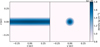 |
Fig. 1 Example of the filament orientation within the simulation box. Shown here on the left-hand side is a slice along the filament axis at y = 0.0 pc and a slice perpendicular of the filament at x = 0.0 pc on the right-hand side. This particular filament has a line-mass of fcyl = 0.25 and a perturbation on the dominant wavelength, which is also the size of the box. |
2.2 Filament perturbation theory
Small perturbations of size ϵ to the variable y along the axis x of hydrostatic isothermal cylinders in a form
![Mathematical equation: $\[y(x, t)=y_0+y_1(x, t)=y_0(1+\epsilon ~\exp (i k x-i \omega t)),\]$](/articles/aa/full_html/2026/04/aa59335-26/aa59335-26-eq16.png) (13)
(13)
will grow for wavelengths λ= 2π/k that are greater than a critical wavelength on a timescale τ = 1/ω (Stodólkiewicz 1963). Perturbations with separations shorter than the critical wavelength will lead to oscillating sound waves within the filament. Although many observed cores on shorter wavelengths could be the result of the formation of the filament, these cores should, in principle, not be able to grow in mass and form cores. The growth timescale has a minimum value for separations that is about double the critical wavelength, also called the dominant wavelength (Nagasawa 1987). Although perturbations can grow on any wavelength longer than the critical one, the fastest growing mode is expected to dominate for small initial perturbations.
Both the critical and dominant wavelengths depend on the line-mass of the filament. For a value of fcyl = 1.0, the critical wavelength is about λcrit = 3.94H and the dominant wavelength is about λdom = 7.82H, with lower values for lower line-masses (Stodólkiewicz 1963; Larson 1985; Nagasawa 1987; Inutsuka & Miyama 1992). Nagasawa (1987) determined the length and timescales for several other values of fcyl, which were interpolated by Fischera & Martin (2012). We use this approximation to determine the fastest growing mode and its growth timescale.
Fischera & Martin (2012) also determined in which values of the filament line-mass, the forming core exceeds the Bonnor-Ebert mass if all the mass on the dominant wavelength is accumulated into the core. This is done by equating the total mass of the dominant wavelength
![Mathematical equation: $\[M_{\mathrm{dom}}=\lambda_{\mathrm{dom}}\left(f_{\mathrm{cyl}}\right) f_{\mathrm{cyl}}\left(\frac{M}{L}\right)_{\mathrm{crit}}\]$](/articles/aa/full_html/2026/04/aa59335-26/aa59335-26-eq17.png) (14)
(14)
to the Bonnor-Ebert mass given by Eq. (12). This shows that if cores are forming on the dominant wavelength, only cores forming in filaments of line-masses 0.20 < fcyl < 0.89 will be able to collapse, a result we test with our simulations.
3 Numerical set-up
Our simulations were run with the code RAMSES (Teyssier 2002), which employs a second-order Godunov scheme on a Cartesian grid to solve the Euler equations in their conservative form. As solver, we chose the MUSCL scheme (Monotonic Upstream-Centred Scheme for Conservation Laws, van Leer 1977) together with the HLLC-Solver (Harten-Lax-van Leer-Contact, Toro et al. 1994) and the multidimensional MC slope limiter (monotonized central-difference, van Leer 1979).
As we study the growth of perturbations within filaments, we set up density profiles according to Eq. (5) with varying line-masses. The filament axis is always aligned with the x-axis and lies in the centre of the y − z plane. In order to minimise accretion to the filament, the background density is always given by a very low particle density of 2.5 cm−3, corresponding to a volume density of 9.87 × 10⁻²⁴ g cm−3 for a molecular weight of μ = 2.36, and contrast to the filament boundary density is set to a value of 103. Therefore, the boundary density is always given by 2.5 × 103 cm−3, or 9.87 × 10⁻²¹ g cm−3, and the central density is set according to Eq. (10). For values above the boundary density, we use an isothermal equation of state with a temperature of 10.0 K. If the density falls below the boundary density, we apply an isobaric equation of state to mimic a constant pressure environment with a value of ![Mathematical equation: $\[p_{ext}=\rho_{b} c_{s}^{2}\]$](/articles/aa/full_html/2026/04/aa59335-26/aa59335-26-eq18.png) , where cs is the isothermal sound speed. An example of filament orientation is given in Fig. 1 where we show two density slices of the initial condition for a line-mass of fcyl = 0.25. The left-hand side shows a slice along the filament axis at y = 0.0 pc and the right-hand side shows a slice perpendicular to the filament axis at x = 0.0 pc.
, where cs is the isothermal sound speed. An example of filament orientation is given in Fig. 1 where we show two density slices of the initial condition for a line-mass of fcyl = 0.25. The left-hand side shows a slice along the filament axis at y = 0.0 pc and the right-hand side shows a slice perpendicular to the filament axis at x = 0.0 pc.
On top of the density profile, we superimpose a perturbation as defined in Eq. (13) of the form
![Mathematical equation: $\[\rho_c(x, t=0.0)=\rho_{c 0}(1+\epsilon ~\cos (2 \pi x / \lambda)),\]$](/articles/aa/full_html/2026/04/aa59335-26/aa59335-26-eq19.png) (15)
(15)
and adapt the scale height in Eq. (6) accordingly. In addition, we include an initial velocity, which we determine by using Eq. (15) in the continuity equation
![Mathematical equation: $\[\frac{\partial \rho}{\partial t}-\nabla\left(\rho v_x\right)=0,\]$](/articles/aa/full_html/2026/04/aa59335-26/aa59335-26-eq20.png) (16)
(16)
which results in a velocity perturbation of
![Mathematical equation: $\[v_{x 1}(x, t=0.0)=-\frac{\epsilon \lambda}{2 \pi \tau} \sin (2 \pi x / \lambda).\]$](/articles/aa/full_html/2026/04/aa59335-26/aa59335-26-eq21.png) (17)
(17)
As one can see, the velocity is shifted by a quarter wavelength compared to the density perturbation and points towards the overdensity. Because of the condition of a constant pressure environment and the relation between the central and boundary density set by Eq. (10), the density perturbation leads to a non-sinusoidal perturbation in the line-mass where the line-mass maximum is given by a line-mass perturbation strength of
![Mathematical equation: $\[\epsilon_f^{\max }=\frac{1-f_0}{f_0}\left(1-\sqrt{\frac{1}{1+\epsilon}}\right),\]$](/articles/aa/full_html/2026/04/aa59335-26/aa59335-26-eq22.png) (18)
(18)
and the line-mass minimum by a line-mass perturbation strength of
![Mathematical equation: $\[\epsilon_f^{\min }=\frac{1-f_0}{f_0}\left(1-\sqrt{\frac{1}{1-\epsilon}}\right).\]$](/articles/aa/full_html/2026/04/aa59335-26/aa59335-26-eq23.png) (19)
(19)
As a result, the line-mass is not strictly conserved. However, even for large values of ϵ this introduces only a small relative error in line-mass. We visualise this in Fig. 2 where the maximum perturbation strength ϵmax is shown to stay below a given relative error threshold in line-mass. These are given by solid, dashed, and dashed-dotted lines, which show the threshold of 1, 2, and 3% relative error, respectively. The values of ϵmax are much higher than the initial perturbation strengths that we typically use in our simulations, which are around 0.01 and less. Therefore, this effect only plays a minor role, as even the error introduced by the discretisation of the filament on the grid can easily reach 1%.
The boundary conditions of the simulation box are set to periodic along the filament axis and to open boundaries in the y and z directions. The periodic condition prevents the filament from collapsing along its axis and allows us to study the growth of density perturbations without the longitudinal collapse or the formation of end cores. This is also the case for filaments in the interstellar medium if they have shallow density gradients at their ends (Hoemann et al. 2023b). The open boundary conditions allow for inflow into the box, which over time can lead to artefacts in the ambient medium. Therefore, we define a cylindrical shell with a radius of half the size of the box in which the density is constantly reset to the background density and the velocity is reset to zero.
We use adaptive mesh refinement with the minimum and maximum resolution of 1283 and 5123 cells, respectively. As refinement threshold, we use the Truelove criterion where the Jeans length has to be resolved by 128 cells (Truelove et al. 1997). The relatively high number of cells guarantees that the central region of the filament is resolved on the highest level, which is more than sufficient to resolve the growing core to a very high degree while leaving the ambient medium at low resolution. We do not use any sink particle formation but stop the simulation as soon as the Jeans length at our highest resolution is not resolved by at least four cells, which indicates the runaway collapse.
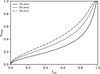 |
Fig. 2 Maximum perturbation strength in dependence of the line-mass in order to keep the relative line-mass error below different thresholds. The thresholds plotted are 1, 2, and 3% given by the solid, dashed, and dashed-dotted lines, respectively. |
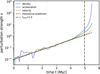 |
Fig. 3 Time evolution of the perturbation strength of different variables, shown as solid lines, compared to the theoretical prediction, given by the dashed line. The blue, cyan, and orange lines show the evolution of the maximum in density, x-acceleration, and x-velocity, respectively, for a filament of a line-mass of fcyl = 0.25. |
4 Simulation results
Here, we discuss the results of our simulations. In the first subsection, we will clarify at which point the Bonnor-Ebert sphere influences the core growth and collapse. In the second subsection, we explore whether the Bonnor-Ebert sphere has an effect on the separation of collapsing cores.
4.1 Non-linear evolution
We systematically explore the core growth on the dominant wavelength for different values of the filament line-mass in order to measure any deviation. Therefore, we set the box size to the dominant wavelength for a given line-mass calculated from the interpolation of Fischera & Martin (2012) and add a single perturbation with the length of the box size. The initial perturbation strength is set to ϵ = 0.01 for low line-masses but is reduced for higher line-masses to give the simulation more time to evolve. For very high line-masses, the dominant wavelength becomes so small that the filament radius would exceed the simulation box. In this case, we double the box size and add a perturbation with a length of half the box size, effectively following the evolution of two peaks on the dominant wavelength.
In Fig. 3 we show the time evolution of the perturbation strength of different variables in a filament with a line-mass of fcyl = 0.25. The blue, cyan, and orange lines show the strength of the measured maximum in density, x-acceleration, and x-velocity, respectively. All perturbed values follow the theoretical prediction shown as a dashed black line and exhibit strong exponential growth at some point; however, the onset of the deviation is not the same. To visualise this more clearly, we determine the absolute relative error of the measured growth rate to the theoretical value of ω. We determine the growth rate in the simulation by taking the time gradient of the logarithm of Eq. (13) where the unperturbed value is first subtracted. For variables whose unperturbed value is zero, such as the acceleration or the velocity, this method has the advantage of not depending on the initial magnitude of the perturbation. As taking the time gradient on an output to output basis introduces strong noise, we first smooth our data by taking a rolling average over five outputs of our simulation. The result is given in Fig. 4 where the colours show the same variables as above. All variables show wave-like patterns in their evolution due to the discretisation of the initial condition, leading to an oscillation in the relative error that dampens over time. One can see that the onset of the non-linear evolution is the same for the density and acceleration but is delayed for the velocity.
In order to determine the respective thresholds in time and line-mass, we measure back from the exponential growth at the end of the simulation and determine when the absolute relative error exceeds a value of 5%. As the density and the acceleration show the same threshold, we use the acceleration as it systematically has a smaller error. Both threshold values, one for the acceleration and one for the velocity, are shown in Fig. 4 as dashed-dotted vertical lines with the respective colour and the corresponding line-mass value at the position of the core is given in the legend. The fact that the non-linear evolution begins before the critical line-mass is reached shows that it is not the loss of radial hydrostatic equilibrium of the filament determining the core evolution or even the collapse. Moreover, the fact that there are two separate thresholds for the acceleration and velocity shows that there seem to be three separate phases in the core evolution. In the first phase, the growth follows linear perturbation theory. In the second phase, the density, and thus the acceleration, grows faster than expected without the velocity changing its behaviour. This means that there is a process that concentrates the density in the core. In the third phase, the velocity shows an exponential deviation. This means that the core collapse has set in and the velocity is growing according to the free-fall collapse.
This effect can also be seen in the evolution of the radial density profile over time. In Fig. 5 we show snapshots of the profile in the three different phases for the filament with a line-mass of fcyl = 0.25. The density and the radius are normalised to a dimensionless form. This means that we can compare the density profiles directly with the general filament profile as defined in Eq. (5), given by the dotted line, and the Bonnor-Ebert sphere profile, shown as a dashed line. In the first phase, plotted as the light blue line, the density profile follows the filament profile. As soon as the filament reaches the second phase as given by the blue line, the density becomes more concentrated and transitions to the Bonnor-Ebert sphere profile. The last snapshot in dark blue shows the density profile just after the second threshold. Here, the profile resembles a Bonnor-Ebert sphere. For later times, the density profile maintains the shape of a Bonnor-Ebert sphere as is expected during collapse (Larson 1969; Penston 1969; Whitworth & Summers 1985; Foster & Chevalier 1993; Keto & Caselli 2010; Naranjo-Romero et al. 2015).
We plot the measured threshold values for all filaments in Fig. 6, where the x-axis shows the overall line-mass of the filament and the y-axis shows the line-mass at the core position at the transition to the respective phase, cyan for the threshold in acceleration and orange for the threshold in velocity. While the threshold in acceleration is line-mass dependent, the threshold in velocity is very similar for lower filament line-masses. Only for larger filament line-masses, both deviations appear very early and therefore the thresholds follow the one-to-one relation shown as the dotted line. Cores forming in filaments with very low line-masses of fcyl = 0.2 and below do not collapse in our simulations, consistent with the lower Bonnor-Ebert mass limit calculated by Fischera & Martin (2012), which we indicate by the dashed-dotted vertical line. Although the thresholds seem to be fitted well from visual inspection, we only performed a single simulation per line-mass. A more rigorous statistical approach would be to perform several simulations for the same line-mass and determine mean values with respective error bars. However, the fitted results seem to be relatively robust with respect to the number of outputs we use to smooth the data and the error threshold we use to determine the beginning of the non-linear deviation.
The first threshold seen in acceleration and density can be explained by the change in the main gravitational potential. As the core grows, its gravitational potential changes from being dominated by the overall filament potential to being dominated by the Bonnor-Ebert sphere potential. This leads to a second order effect where the core is more strongly concentrated to its centre. Therefore, the perturbation grows faster than expected. We can determine the expected transition line-mass at the core position by assuming that the Bonnor-Ebert sphere potential of the perturbation should be deeper than the overall filament potential even for the core’s largest extent, which is given by the unperturbed filament radius R
![Mathematical equation: $\[\Phi_{\mathrm{BE}}(R)>\Phi_{\mathrm{cyl}}(R).\]$](/articles/aa/full_html/2026/04/aa59335-26/aa59335-26-eq24.png) (20)
(20)
We calculate the potential of the filament, as well as the Bonnor-Ebert sphere, by computing the numerical solution to Eqs. (4) and (11) using the explicit fifth-order Runge-Kutta method built into the SciPy integrate package. For the same central density, the filament potential is deeper than the Bonnor-Ebert sphere potential at all radii. We then iteratively determine how large the central density of the Bonnor-Ebert sphere has to be in order to fulfill the condition given by Eq. (20) and use it to calculate the corresponding line-mass value fcore given by Eq. (5). The result is shown in Fig. 6 as the solid line. As one can see, the cyan values closely follow this prediction, except for line-masses higher than fcyl = 0.65 where the deviation seems to be instantaneous.
Likewise, the threshold in velocity can be explained by assuming that it is the Bonnor-Ebert sphere that also determines the collapse of the core. As the maximum supported mass of a Bonnor-Ebert sphere in Eq. (12) is given by the external pressure, one can estimate at which line-mass threshold the mass within a core exceeds this maximum value. However, the external pressure is not simply given by the external medium around the filament but is considerably larger since the core sits within the filament itself. This means that we have to determine the total mass of the core, as well as the average pressure on its surface. However, this is not trivial because a core located within a filament is typically neither spherical nor has a clearly defined surface. We therefore make use of some simplifications. On the one hand, we estimate the mass of a core by numerically integrating the mass of a spherical region centred inside an unperturbed filamentary density distribution as given by Eq. (5)
![Mathematical equation: $\[M_{\mathrm{core}}=\int_0^R \int_0^\pi \int_0^{2 \pi} \frac{\rho_c r^2 ~\sin (\theta) \mathrm{d} r \mathrm{~d} \theta \mathrm{~d} \phi}{\left(1+r^2\left(1-\cos (\theta)^2\right) / H^2\right)^2},\]$](/articles/aa/full_html/2026/04/aa59335-26/aa59335-26-eq25.png) (21)
(21)
where we expressed the cylindrical radius in spherical coordinates r, θ, and ϕ. On the other hand, we estimate the average external pressure at the surface of this region via the density, which we get by solving the surface integral numerically and normalising by the surface area
![Mathematical equation: $\[\left\langle\rho_{\mathrm{BE}}\right\rangle=\frac{1}{4 \pi R^2} \int_0^\pi \int_0^{2 \pi} \frac{\rho_c R^2 ~\sin (\theta) \mathrm{d} \theta \mathrm{~d} \phi}{\left(1+R^2\left(1-\cos (\theta)^2\right) / H^2\right)^2}.\]$](/articles/aa/full_html/2026/04/aa59335-26/aa59335-26-eq26.png) (22)
(22)
For the radius, we used the maximum volume that a core can occupy. Generally, this value is given by the filament radius. However, for large line-masses the dominant wavelength becomes smaller than the filament diameter. This means that the core radius can at maximum be half the distance to the next core. We therefore define the core radius as the minimum value of this value and the unperturbed filament radius. These simplifications neglect that a core represents an overdensity within the filament. Thus, the density at the surface and mass within the core should be larger than for the initial filament. However, this effect is somewhat counterbalanced, as both the mass within the core and the density at its surface should increase in an analogous manner for self-similar profiles like the Bonnor-Ebert sphere.
We plot both masses as functions of the line-mass in Fig. 7, where the integrated mass is given by the dark blue solid line and the maximum supported mass calculated by using the average surface density in Eq. (12) is given as a dark blue dashed-dotted line. We did not include a y-axis as all masses scale the same with respect to the external pressure. Therefore, the calculation is scale-free. As can be seen, the mass within the core surpasses the supported Bonnor-Ebert mass at fcyl = 0.66, indicated as a dashed vertical line, which is exactly the value we plot as a dashed horizontal line in Fig. 6. Thus, as soon as the perturbation reaches this threshold, collapse will set in. If the initial line-mass is already above this value, any perturbation will lead to a collapsing core. This is the reason why we observe a direct transition to the exponential increase in Fig. 6 for the line-mass values above fcyl = 0.60. For very large line-masses, one can see a break in the curves as the core distances on the dominant perturbation wavelength become smaller than the filament diameter.
For comparison, we also plot the total mass contained in the dominant wavelength compared to the Bonnor-Ebert mass supported by the external pressure as grey solid and dashed-dotted lines. The intersections show the calculation of Fischera & Martin (2012) where only the line-masses of the values 0.20 < fcyl < 0.89 form collapsing cores. Despite approaching the same value for low line-mass, the internal pressure reduces the supported mass to smaller and smaller values compared to the external pressure as the line-mass grows. This is due to the density profile, which is flat at low line-masses and increasingly steeper at larger line-masses. Here, one can also see that the constraint on the core radius as described above limits the mass within the core to the maximum mass within the dominant wavelength. Therefore, the solid dark blue line follows the solid grey line. However, this does not influence the collapse, as both masses, the core mass and the supported mass, fall steeply. Thus, the internal pressure can also demonstrate why cores forming within high line-mass filaments are even able to collapse, which cannot be explained by the external pressure, as shown by the cyan lines. It is not the total mass of the dominant wavelength that determines the collapse but the local Bonnor-Ebert mass within the filament.
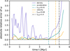 |
Fig. 4 Time evolution of the absolute relative error of the growth time scale ω measured in the simulation for a line-mass of fcyl = 0.25. The solid blue, cyan, and orange line shows the error of the density, x-acceleration and x-velocity, respectively. We define the beginning of the non-linear evolution by determining the point in time when the error exceeds a value of 5% when measuring back from the end of the simulation. The thresholds are indicated by the vertical dashed-dotted lines, for which we also determine the line-masses at the position of the core, which are given in the legend. |
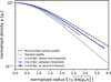 |
Fig. 5 Evolution of the radial density profile of the core from the linear growth phase until the start of the collapse for a line-mass of fcyl = 0.25. Shown are snapshots before the first threshold in light blue, between the first and second threshold in blue, and just after the second threshold in dark blue. The density and the radius are normalised to a dimensionless form to compare profiles with different concentrations. The filament profile as defined in Eq. (5) is given as a dotted line and the Bonnor-Ebert sphere profile as a dashed line. |
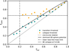 |
Fig. 6 Threshold line-masses at the position of the core in dependence of the filament line-mass fcyl. The beginning of the non-linear evolution in acceleration is given by the cyan points, for the velocity by the orange points. The solid line indicates where the Bonnor-Ebert sphere potential dominates over the filament potential. The vertical dashed-dotted line shows the lower mass limit for a collapsing Bonnor-Ebert sphere and the horizontal dashed line shows the result of calculating the maximum supported Bonnor-Ebert mass assuming a external pressure given by the density within the filament. |
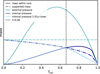 |
Fig. 7 Comparison of the mass within a core, given by the solid lines, to the supported Bonnor-Ebert mass, given by the dashed-dotted lines, as function of the line-mass. The cyan lines show the model of only taking the external pressure into account where the core mass is given by the total mass of the dominant wavelength. The dark blue lines show our model of a spherical core located within a filamentary density profile where cores become unstable for line-masses above fcyl = 0.66, as marked by the vertical dashed line. The light blue lines show the closest separation the cores can have while still being unstable, which is 2.61 times closer than the dominant wavelength. |
4.2 Effects on the separation of collapsing cores
If the collapse is thus given by a local Bonnor-Ebert criterion, the question arises of whether stars can form on any given core separation. However, there is an upper limit on how close unstable cores can form, given by the maximum size they occupy. Due to our constraint that the core radius is given by the minimum of the filament radius and half the distance to the next core, the mass within the core reduces faster than the average ambient density for shorter and shorter core separations. The transition point where one cannot find any unstable cores anymore is shown by the light blue lines in Fig. 7, which is the case for cores spaced 2.61 times closer than the dominant wavelength. At this value, cores are also separated closer than the critical wavelength. This means that while small perturbations will not be able to grow into unstable cores, large line-mass perturbations that exceed the collapse threshold of fcyl = 0.66, and at the same time lead to a dominant Bonnor-Ebert sphere potential, should be able to collapse. We plot this limit in Fig. 8 in terms of minimum line-mass perturbation strength as a dashed black line. We also include the upper limit of a line-mass of fcyl = 1.0 as a solid black line.
We test this prediction by simulating high line-mass filaments with varying perturbation wavelengths and compare if the cores collapse on the wavelength of the dominant mode or on the separation given by the initial condition. In contrast to the former simulations that used a perturbation in density, here we use a perturbation in line-mass. This is due to the fact that a large change in line-mass cannot be adequately reproduced with a linear perturbation in density, as given by Eq. (18). For large changes in line-mass as shown in Fig. 8, the linear perturbation strength ϵ even exceeds values of 1.0 and the resulting initial condition would not be a continuous filament. Therefore, a large line-mass perturbation means that our simulation already begins in the non-linear regime, where we cannot derive a self-consistent initial condition in velocity. Nevertheless, we are only interested if large line-mass perturbations can lead to core collapse on shorter wavelengths than allowed by linear growth. This is also exactly the initial condition that arises when filaments form in molecular clouds with large variations in line-mass. Thus, we neglect any initial velocity along the filament and set up the density profile consistent with Eq. (10).
We show the test cases and their outcomes in Fig. 9 where the dominant and critical wavelength are given in units of the full width at half maximum (FWHM) of the filament profile as defined in (Fischera & Martin 2012). The dominant wavelength is shown by the solid black line and the critical wavelength, about a factor of two shorter, as the dashed black line, respectively. We also plot the 3D Jeans length defined by the central density
![Mathematical equation: $\[\lambda_J=\sqrt{\frac{\pi c_s^2}{G \rho_c}},\]$](/articles/aa/full_html/2026/04/aa59335-26/aa59335-26-eq27.png) (23)
(23)
as the dotted black line. The Bonnor-Ebert sphere correction of a factor of 2.61 shorter than the dominant wavelength is indicated by the blue solid line. We simulate filaments with perturbation lengths towards longer and shorter separations compared to this value by setting up line-mass perturbations with one third and half the dominant wavelength. In addition, we also set up perturbations which are 2.22 and 2.5 times shorter than the dominant wavelength by doubling the box size, and reducing the box size by a factor of 0.9 and 0.8. If only one collapsing core forms, the wavelength on the scale of the box size was able to grow faster and, therefore, the dominant wavelength is the fastest growing mode. The dark blue dots indicate simulations where all cores collapse on the initial perturbation length, and the light blue dots show simulations where only one core collapses.
As one can see, all of our test cases with wavelengths above but close to the Bonnor-Ebert collapse threshold are able to trigger direct collapse of cores, even if their separation lies below the critical wavelength. However, modes of one third of the dominant wavelength do not collapse directly in our simulations but form a collapsing core on the dominant wavelength. Both evolutions, the collapse of the initial mode and of the dominant mode, are shown in Fig. 10 for a filament with fcyl = 0.9. Here we plot the evolution of the maximum line-mass within the filament as a function of time. The light blue line shows the evolution of the mode three times shorter and the dark blue line shows the evolution of the mode 2.22 times shorter than the dominant wavelength. While the cores for the dark blue case rapidly grow and collapse in a very short time, the cores for the light blue case show a soundwave oscillation despite having line-masses that consistently exceed the critical value of where the filament should be radially stable. There is no collapse until a larger core grows on the dominant wavelength, which eventually collapses after one Myr. This demonstrates that core collapse is indeed not caused by the loss of radial stability but by the mass exceeding the local collapse threshold.
In order to make sure that it is not the perturbation strength that prevents the collapse in the cases where the dominant mode wins, we set it close to the maximum possible value where the perturbed initial filament line-mass approaches 1.0. This is visualised in Fig. 8 as light blue dots. In contrast, the initial perturbation strength for the simulations where the initial mode collapses directly is shown as dark blue dots. While we expect that cores should be able to directly collapse if the perturbation strength is above the dashed threshold value, we notice that low initial strengths close to this threshold are not able to overcome the restoring forces leading to oscillating sound waves. The reason for this is likely due to the initial conditions. On the one hand, the threshold value of fcyl = 0.66 was measured by the growth of linear perturbations. As we only use an initial perturbation in line-mass, the missing inflow velocity along the filament could be increasing the perturbation strength needed for direct collapse. On the other hand, the initial perturbation is not set up as a Bonnor-Ebert sphere. This means that the overdensity needs time to adjust to a Bonnor-Ebert sphere profile to collapse. As this happens on the timescale of a sound crossing time, the filament first enters a phase of oscillating overdensities. We observe this effect in some simulations with low initial perturbation strength where there is a long period of oscillating soundwaves before the cores eventually do collapse on the initial mode.
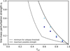 |
Fig. 8 Minimum and maximum line-mass perturbation strength for direct collapse as function of the filament line-mass. The minimum is given by the fact that the Bonnor-Ebert sphere potential has to dominate over the filament potential and at the same time the line-mass maximum has to be above fcyl = 0.66. The maximum is given by the fact that the line-mass cannot exceed a value of 1.0 in equilibrium. The light and dark blue dots show the perturbation strength we used for our test simulations given in Fig. 9. |
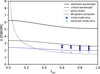 |
Fig. 9 Bonnor-Ebert sphere collapse threshold, shown as the blue solid line, in comparison to the dominant and critical wavelength, given by the black solid and dashed lines, respectively. The wavelengths are given in units of the FWHM of the filament profile. We assess the threshold by performing test simulations indicated by markers where the colour indicates if the initial perturbation is preserved during collapse, given by the dark blue markers, or if it is lost and a collapsing core forms on the dominant wavelength, as shown by the light blue markers. |
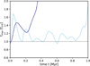 |
Fig. 10 Evolution of the maximum line-mass in the simulation of a filament of fcyl = 0.9 for a perturbation wavelength of three times shorter, shown in light blue, and 2.22 times shorter, shown in dark blue, than the dominant wavelength. In the former case the core does not collapse directly but the line-mass oscillates with values above the critical line-mass until eventually a single collapsing core forms on the dominant wavelength. |
5 Conclusions and discussion
We show that if cores form with enough mass, they can collapse even if they lie closer together than the minimum wavelength for core growth given by linear perturbation theory. Our results help to explain why some observations show filaments with star-forming cores, which are separated closer than the dominant wavelength. Instead of collapsing due to linear growth, these cores could have formed as large line-mass perturbations during filament formation. Moreover, they could also explain why some observations show hierarchical fragmentation. Low line-mass filaments should form dense, high line-mass perturbations on the dominant scale. As soon as it reaches the line-mass threshold for direct collapse, any left-over overdensity within these regions is highly susceptible to collapse in very short separations. Although our results do not allow for the collapse on the exact value of the Jeans length set by the central density, our derived wavelength threshold is very similar and would be hard to distinguish observationally. In summary, our main conclusions are the following.
Perturbation growth in filaments shows non-linear effects as soon as the Bonnor-Ebert sphere gravitationally dominates over the filament potential. As a result, the profile becomes more concentrated and therefore the density evolves faster than predicted by linear growth.
Core collapse, as indicated by the non-linear evolution of the velocity along the filament axis, sets in before the perturbation reaches the critical line-mass. This means that core collapse is not triggered by loss of radial stability of the filament.
We can explain the early collapse by assuming that the mass within the core has reached the Bonnor-Ebert mass limit given by the pressure within the filament. This sets the collapse threshold to a line-mass value of fcyl = 0.66.
For large enough line-mass perturbations, cores therefore can go into direct collapse even if their separation is closer than the minimum wavelength required for perturbation growth. We predict that this separation can nominally be 2.61 times closer than the dominant wavelength.
The main caveat of our study is that we do not measure the collapse threshold of fcyl = 0.66 with high accuracy. From a theoretical standpoint, one could also argue for a collapse threshold of fcyl = 0.73 as this is the line-mass when the density contrast according to Eq. (10) from central to boundary density within a filament reaches the value required for collapse of a Bonnor-Ebert sphere of 14.1. We test this possibility by measuring if the contrast of central to boundary density actually reaches this value in our simulations before the cores collapse. However, this does not seem to be the case. For initial filament line-masses below fcyl = 0.73 the core collapse begins before the density contrast reaches a value of 14.1. Therefore, it is indeed a mass threshold and not a density contrast which triggers the beginning of collapse. Nevertheless, a slight shift to larger line-mass values in the collapse threshold also only leads to a minor shift to larger values of the minimum wavelength for direct collapse.
A central question for our scenario is whether filaments form with large enough line-mass perturbations to trigger direct collapse. Observationally, it is not easy to distinguish overdensities that have formed with high line-mass from those that have grown to large values. However, detected line-mass deviations in filaments are quite large. For example, Roy et al. (2015) find a standard deviation in line-masses of 7%, which locally also reaches values of up to 30%. Considering that most observed filaments are also rather large in line-mass, the perturbation strengths required to go into direct collapse are not that high, as can be seen in Fig. 8.
Acknowledgements
This research was supported by the Excellence Cluster ORIGINS which is funded by the Deutsche Forschungsgemeinschaft (DFG, German Research Foundation) under Germany’s Excellence Strategy - EXC-2094 - 390783311.
References
- Alves, J. F., Lada, C. J., & Lada, E. A. 2001, Nature, 409, 159 [NASA ADS] [CrossRef] [Google Scholar]
- André, P., Men’shchikov, A., Bontemps, S., et al. 2010, A&A, 518, L102 [NASA ADS] [CrossRef] [EDP Sciences] [Google Scholar]
- Bastien, P. 1983, A&A, 119, 109 [NASA ADS] [Google Scholar]
- Beuther, H., Ragan, S. E., Johnston, K., et al. 2015, A&A, 584, A67 [NASA ADS] [CrossRef] [EDP Sciences] [Google Scholar]
- Bonnor, W. B. 1956, MNRAS, 116, 351 [NASA ADS] [CrossRef] [Google Scholar]
- Burkert, A., & Hartmann, L. 2004, ApJ, 616, 288 [Google Scholar]
- Busquet, G., Zhang, Q., Palau, A., et al. 2013, ApJ, 764, L26 [NASA ADS] [CrossRef] [Google Scholar]
- Cao, Y., Qiu, K., Zhang, Q., & Li, G.-X. 2022, ApJ, 927, 106 [NASA ADS] [CrossRef] [Google Scholar]
- Chung, E. J., Lee, C. W., Kim, S., et al. 2024, ApJ, 970, 122 [Google Scholar]
- Clarke, S. D., & Whitworth, A. P. 2015, MNRAS, 449, 1819 [NASA ADS] [CrossRef] [Google Scholar]
- Clarke, S. D., Whitworth, A. P., & Hubber, D. A. 2016, MNRAS, 458, 319 [CrossRef] [Google Scholar]
- Contreras, Y., Garay, G., Rathborne, J. M., & Sanhueza, P. 2016, MNRAS, 456, 2041 [CrossRef] [Google Scholar]
- Coughlin, E. R., & Nixon, C. J. 2020, ApJS, 247, 51 [Google Scholar]
- Ebert, R. 1955, ZAp, 37, 217 [Google Scholar]
- Fiege, J. D., & Pudritz, R. E. 2000, MNRAS, 311, 105 [NASA ADS] [CrossRef] [Google Scholar]
- Fischera, J., & Martin, P. G. 2012, A&A, 542, A77 [NASA ADS] [CrossRef] [EDP Sciences] [Google Scholar]
- Foster, P. N., & Chevalier, R. A. 1993, ApJ, 416, 303 [NASA ADS] [CrossRef] [Google Scholar]
- Gehman, C. S., Adams, F. C., Fatuzzo, M., & Watkins, R. 1996a, ApJ, 457, 718 [NASA ADS] [CrossRef] [Google Scholar]
- Gehman, C. S., Adams, F. C., & Watkins, R. 1996b, ApJ, 472, 673 [NASA ADS] [CrossRef] [Google Scholar]
- Gritschneder, M., Heigl, S., & Burkert, A. 2017, ApJ, 834, 202 [Google Scholar]
- Hacar, A., Clark, S. E., Heitsch, F., et al. 2023, ASP Conf. Ser., 534, 153 [NASA ADS] [Google Scholar]
- Hanawa, T., Kudoh, T., & Tomisaka, K. 2019, ApJ, 881, 97 [NASA ADS] [CrossRef] [Google Scholar]
- Hartmann, L. 2002, ApJ, 578, 914 [Google Scholar]
- He, Y.-X., Liu, H.-L., Tang, X.-D., et al. 2023, ApJ, 957, 61 [NASA ADS] [CrossRef] [Google Scholar]
- Heigl, S., Hoemann, E., & Burkert, A. 2022, MNRAS, 517, 5272 [Google Scholar]
- Henshaw, J. D., Caselli, P., Fontani, F., et al. 2016, MNRAS, 463, 146 [NASA ADS] [CrossRef] [Google Scholar]
- Hoemann, E., Heigl, S., & Burkert, A. 2023a, MNRAS, 521, 5152 [Google Scholar]
- Hoemann, E., Heigl, S., & Burkert, A. 2023b, MNRAS, 525, 3998 [NASA ADS] [CrossRef] [Google Scholar]
- Hosseinirad, M., Naficy, K., Abbassi, S., & Roshan, M. 2017, MNRAS, 465, 1645 [Google Scholar]
- Hosseinirad, M., Abbassi, S., Roshan, M., & Naficy, K. 2018, MNRAS, 475, 2632 [Google Scholar]
- Hwang, J., Sanhueza, P., Girart, J. M., et al. 2026, AJ, 171, 50 [Google Scholar]
- Inutsuka, S.-I., & Miyama, S. M. 1992, ApJ, 388, 392 [CrossRef] [Google Scholar]
- Jackson, J. M., Finn, S. C., Chambers, E. T., Rathborne, J. M., & Simon, R. 2010, ApJ, 719, L185 [Google Scholar]
- Kainulainen, J., Ragan, S. E., Henning, T., & Stutz, A. 2013, A&A, 557, A120 [NASA ADS] [CrossRef] [EDP Sciences] [Google Scholar]
- Kainulainen, J., Hacar, A., Alves, J., et al. 2016, A&A, 586, A27 [NASA ADS] [CrossRef] [EDP Sciences] [Google Scholar]
- Kainulainen, J., Stutz, A. M., Stanke, T., et al. 2017, A&A, 600, A141 [NASA ADS] [CrossRef] [EDP Sciences] [Google Scholar]
- Keto, E., & Caselli, P. 2010, MNRAS, 402, 1625 [Google Scholar]
- Könyves, V., André, P., Men’shchikov, A., et al. 2015, A&A, 584, A91 [Google Scholar]
- Könyves, V., André, P., Arzoumanian, D., et al. 2020, A&A, 635, A34 [Google Scholar]
- Larson, R. B. 1969, MNRAS, 145, 271 [Google Scholar]
- Larson, R. B. 1985, MNRAS, 214, 379 [NASA ADS] [Google Scholar]
- Liu, H.-L., Stutz, A., & Yuan, J.-H. 2018, MNRAS, 478, 2119 [NASA ADS] [CrossRef] [Google Scholar]
- Lu, X., Zhang, Q., Liu, H. B., Wang, J., & Gu, Q. 2014, ApJ, 790, 84 [NASA ADS] [CrossRef] [Google Scholar]
- Lu, X., Zhang, Q., Liu, H. B., et al. 2018, ApJ, 855, 9 [Google Scholar]
- Mattern, M., Kainulainen, J., Zhang, M., & Beuther, H. 2018, A&A, 616, A78 [NASA ADS] [CrossRef] [EDP Sciences] [Google Scholar]
- McLaughlin, D. E., & Pudritz, R. E. 1996, ApJ, 469, 194 [Google Scholar]
- Miettinen, O. 2012, A&A, 540, A104 [NASA ADS] [CrossRef] [EDP Sciences] [Google Scholar]
- Miettinen, O., Mattern, M., & André, P. 2022, A&A, 667, A90 [NASA ADS] [CrossRef] [EDP Sciences] [Google Scholar]
- Molinari, S., Swinyard, B., Bally, J., et al. 2010, A&A, 518, L100 [NASA ADS] [CrossRef] [EDP Sciences] [Google Scholar]
- Moon, S., & Ostriker, E. C. 2024, ApJ, 975, 295 [Google Scholar]
- Moon, S., & Ostriker, E. C. 2025, ApJ, 987, 78 [Google Scholar]
- Nagasawa, M. 1987, Prog. Theor. Phys., 77, 635 [CrossRef] [Google Scholar]
- Naranjo-Romero, R., Vázquez-Semadeni, E., & Loughnane, R. M. 2015, ApJ, 814, 48 [NASA ADS] [CrossRef] [Google Scholar]
- Ostriker, J. 1964, ApJ, 140, 1056 [Google Scholar]
- Palau, A., Zapata, L. A., Román-Zúniga, C. G., et al. 2018, ApJ, 855, 24 [NASA ADS] [CrossRef] [Google Scholar]
- Penston, M. V. 1969, MNRAS, 144, 425 [NASA ADS] [CrossRef] [Google Scholar]
- Pon, A., Toalá, J. A., Johnstone, D., et al. 2012, ApJ, 756, 145 [NASA ADS] [CrossRef] [Google Scholar]
- Roy, A., André, P., Arzoumanian, D., et al. 2015, A&A, 584, A111 [NASA ADS] [CrossRef] [EDP Sciences] [Google Scholar]
- Schneider, S., & Elmegreen, B. G. 1979, ApJS, 41, 87 [Google Scholar]
- Shu, F. H. 1977, ApJ, 214, 488 [Google Scholar]
- Stodólkiewicz, J. S. 1963, Acta Astron., 13, 30 [NASA ADS] [Google Scholar]
- Svoboda, B. E., Shirley, Y. L., Traficante, A., et al. 2019, ApJ, 886, 36 [Google Scholar]
- Tafalla, M., & Hacar, A. 2015, A&A, 574, A104 [NASA ADS] [CrossRef] [EDP Sciences] [Google Scholar]
- Tafalla, M., Myers, P. C., Caselli, P., & Walmsley, C. M. 2004, A&A, 416, 191 [NASA ADS] [CrossRef] [EDP Sciences] [Google Scholar]
- Takahashi, S., Ho, P. T. P., Teixeira, P. S., Zapata, L. A., & Su, Y.-N. 2013, apj, 763, 57 [Google Scholar]
- Teixeira, P. S., Takahashi, S., Zapata, L. A., & Ho, P. T. P. 2016, A&A, 587, A47 [NASA ADS] [CrossRef] [EDP Sciences] [Google Scholar]
- Teyssier, R. 2002, A&A, 385, 337 [CrossRef] [EDP Sciences] [Google Scholar]
- Toro, E., Spruce, M., & Speares, W. 1994, Shock Waves, 4, 25 [NASA ADS] [CrossRef] [Google Scholar]
- Truelove, J. K., Klein, R. I., McKee, C. F., et al. 1997, ApJ, 489, L179 [CrossRef] [Google Scholar]
- van Leer, B. 1977, J. Comput. Phys., 23, 276 [Google Scholar]
- van Leer, B. 1979, J. Comput. Phys., 32, 101 [Google Scholar]
- Vázquez-Semadeni, E., Kim, J., Shadmehri, M., & Ballesteros-Paredes, J. 2005, ApJ, 618, 344 [CrossRef] [Google Scholar]
- Vázquez-Semadeni, E., Palau, A., Ballesteros-Paredes, J., Gómez, G. C., & Zamora-Avilés, M. 2019, MNRAS, 490, 3061 [Google Scholar]
- Wang, K., Zhang, Q., Testi, L., et al. 2014, MNRAS, 439, 3275 [Google Scholar]
- Whitworth, A., & Summers, D. 1985, MNRAS, 214, 1 [Google Scholar]
- Williams, G. M., Peretto, N., Avison, A., Duarte-Cabral, A., & Fuller, G. A. 2018, A&A, 613, A11 [NASA ADS] [CrossRef] [EDP Sciences] [Google Scholar]
- Yang, D., Liu, H.-L., Liu, T., et al. 2024, ApJ, 976, 241 [Google Scholar]
- Zhang, G.-Y., André, P., Men’shchikov, A., & Wang, K. 2020, A&A, 642, A76 [NASA ADS] [CrossRef] [EDP Sciences] [Google Scholar]
- Zhen, L. M., Liu, H.-L., Lu, X., et al. 2025, A&A, 700, A47 [NASA ADS] [CrossRef] [EDP Sciences] [Google Scholar]
- Zhou, C., Zhu, M., Yuan, J., et al. 2019, MNRAS, 485, 3334 [NASA ADS] [CrossRef] [Google Scholar]
All Figures
|
Fig. 1 Example of the filament orientation within the simulation box. Shown here on the left-hand side is a slice along the filament axis at y = 0.0 pc and a slice perpendicular of the filament at x = 0.0 pc on the right-hand side. This particular filament has a line-mass of fcyl = 0.25 and a perturbation on the dominant wavelength, which is also the size of the box. |
| In the text | |
|
Fig. 2 Maximum perturbation strength in dependence of the line-mass in order to keep the relative line-mass error below different thresholds. The thresholds plotted are 1, 2, and 3% given by the solid, dashed, and dashed-dotted lines, respectively. |
| In the text | |
|
Fig. 3 Time evolution of the perturbation strength of different variables, shown as solid lines, compared to the theoretical prediction, given by the dashed line. The blue, cyan, and orange lines show the evolution of the maximum in density, x-acceleration, and x-velocity, respectively, for a filament of a line-mass of fcyl = 0.25. |
| In the text | |
|
Fig. 4 Time evolution of the absolute relative error of the growth time scale ω measured in the simulation for a line-mass of fcyl = 0.25. The solid blue, cyan, and orange line shows the error of the density, x-acceleration and x-velocity, respectively. We define the beginning of the non-linear evolution by determining the point in time when the error exceeds a value of 5% when measuring back from the end of the simulation. The thresholds are indicated by the vertical dashed-dotted lines, for which we also determine the line-masses at the position of the core, which are given in the legend. |
| In the text | |
|
Fig. 5 Evolution of the radial density profile of the core from the linear growth phase until the start of the collapse for a line-mass of fcyl = 0.25. Shown are snapshots before the first threshold in light blue, between the first and second threshold in blue, and just after the second threshold in dark blue. The density and the radius are normalised to a dimensionless form to compare profiles with different concentrations. The filament profile as defined in Eq. (5) is given as a dotted line and the Bonnor-Ebert sphere profile as a dashed line. |
| In the text | |
|
Fig. 6 Threshold line-masses at the position of the core in dependence of the filament line-mass fcyl. The beginning of the non-linear evolution in acceleration is given by the cyan points, for the velocity by the orange points. The solid line indicates where the Bonnor-Ebert sphere potential dominates over the filament potential. The vertical dashed-dotted line shows the lower mass limit for a collapsing Bonnor-Ebert sphere and the horizontal dashed line shows the result of calculating the maximum supported Bonnor-Ebert mass assuming a external pressure given by the density within the filament. |
| In the text | |
|
Fig. 7 Comparison of the mass within a core, given by the solid lines, to the supported Bonnor-Ebert mass, given by the dashed-dotted lines, as function of the line-mass. The cyan lines show the model of only taking the external pressure into account where the core mass is given by the total mass of the dominant wavelength. The dark blue lines show our model of a spherical core located within a filamentary density profile where cores become unstable for line-masses above fcyl = 0.66, as marked by the vertical dashed line. The light blue lines show the closest separation the cores can have while still being unstable, which is 2.61 times closer than the dominant wavelength. |
| In the text | |
|
Fig. 8 Minimum and maximum line-mass perturbation strength for direct collapse as function of the filament line-mass. The minimum is given by the fact that the Bonnor-Ebert sphere potential has to dominate over the filament potential and at the same time the line-mass maximum has to be above fcyl = 0.66. The maximum is given by the fact that the line-mass cannot exceed a value of 1.0 in equilibrium. The light and dark blue dots show the perturbation strength we used for our test simulations given in Fig. 9. |
| In the text | |
|
Fig. 9 Bonnor-Ebert sphere collapse threshold, shown as the blue solid line, in comparison to the dominant and critical wavelength, given by the black solid and dashed lines, respectively. The wavelengths are given in units of the FWHM of the filament profile. We assess the threshold by performing test simulations indicated by markers where the colour indicates if the initial perturbation is preserved during collapse, given by the dark blue markers, or if it is lost and a collapsing core forms on the dominant wavelength, as shown by the light blue markers. |
| In the text | |
|
Fig. 10 Evolution of the maximum line-mass in the simulation of a filament of fcyl = 0.9 for a perturbation wavelength of three times shorter, shown in light blue, and 2.22 times shorter, shown in dark blue, than the dominant wavelength. In the former case the core does not collapse directly but the line-mass oscillates with values above the critical line-mass until eventually a single collapsing core forms on the dominant wavelength. |
| In the text | |
Current usage metrics show cumulative count of Article Views (full-text article views including HTML views, PDF and ePub downloads, according to the available data) and Abstracts Views on Vision4Press platform.
Data correspond to usage on the plateform after 2015. The current usage metrics is available 48-96 hours after online publication and is updated daily on week days.
Initial download of the metrics may take a while.