| Issue |
A&A
Volume 710, June 2026
|
|
|---|---|---|
| Article Number | A53 | |
| Number of page(s) | 21 | |
| Section | Planets, planetary systems, and small bodies | |
| DOI | https://doi.org/10.1051/0004-6361/202556764 | |
| Published online | 28 May 2026 | |
Resonant structures in exozodiacal clouds created by exo-Earths in the habitable zone of late-type stars
1
Department of Physics and Astronomy, Seoul National University,
1 Gwanak-ro,
Gwanak-gu,
Seoul
08826,
Republic of Korea
2
SNU Astronomy Research Center, Department of Physics and Astronomy, Seoul National University,
1 Gwanak-ro,
Gwanak-gu,
Seoul
08826,
Republic of Korea
★ Corresponding authors: This email address is being protected from spambots. You need JavaScript enabled to view it.
; This email address is being protected from spambots. You need JavaScript enabled to view it.
Received:
6
August
2025
Accepted:
13
April
2026
Abstract
Context. Earth-like exoplanets can create resonant structures in exozodiacal dust through mean motion resonances. These structures not only suggest the presence of such planets but also act as potential noise sources in future mid-infrared nulling interferometry observations.
Aims. We aim to investigate how resonant structures in exozodiacal dust vary across stellar spectral types (F4-M4) and evaluate how stellar wind drag affects their morphology and brightness in mature planetary systems.
Methods. We conducted numerical simulations of dust dynamics, extending earlier studies by including spectral-type variation in stellar wind drag in addition to Poynting-Robertson (PR) drag. Our models represent systems of a few gigayears hosting an Earth-like exoplanet in the habitable zone. We produced spatially resolved maps of optical depth and thermal emission for different stellar spectral types.
Results. Our simulations show that resonant ring structures form for all stellar spectral types considered. In particular, we find that stellar wind drag plays a critical role in shaping dust dynamics around old M-type stars, where it could dominate over PR drag by a factor of approximately 44. This reduces the contrast of resonant rings relative to the background disk compared to cases with a stellar wind fixed at the solar value. Across spectral types, the geometric optical depth contrast for resonant rings increases toward lower-mass stars, assuming a background level fixed at 3 zodis. Our calculations show that the optical depth and thermal emission distributions at 10 μm are asymmetric in resonant rings, and we quantified the resulting magnitude of asymmetric brightness.
Conclusions. Our findings highlight the importance of incorporating both resonant dynamics and stellar wind effects when modeling exozodiacal dust around stars of different spectral types.
Key words: radiation: dynamics / methods: numerical / planets and satellites: terrestrial planets / planet-disk interactions / zodiacal dust / stars: winds, outflows
© The Authors 2026
 Open Access article, published by EDP Sciences, under the terms of the Creative Commons Attribution License (https://creativecommons.org/licenses/by/4.0), which permits unrestricted use, distribution, and reproduction in any medium, provided the original work is properly cited.
This article is published in open access under the Subscribe to Open model. This email address is being protected from spambots. You need JavaScript enabled to view it. to support open access publication.
1 Introduction
Dust particles in debris disks can form resonant structures through interactions with planets. As the particles spiral inward under the influence of Poynting-Robertson (PR) and stellar wind drags, they may become trapped in mean motion resonances (MMRs), yielding enhanced densities along resonant orbits (Liou & Zook 1997; Kuchner & Holman 2003; Kuchner et al. 2007; Pástor et al. 2009; Shannon et al. 2015). In the Solar System, such structures are exemplified by Earth’s resonant ring (Jackson & Zook 1989; Dermott et al. 1994; Sommer et al. 2020). This structure has been observationally confirmed in the infrared by space telescopes such as IRAS and COBE/DIRBE (Dermott et al. 1984; Reach et al. 1995). Similar processes can take place in extrasolar systems, producing asymmetric ring structures in exo-zodiacal dust (exozodi) near planetary orbits (Kral et al. 2017; Pearce 2026; Currie et al. 2025).
As extrasolar analogs of the zodiacal dust, exozodis can be a critical foreground for the detection of potentially habitable exoplanets. Located near the habitable zone (HZ), warm exozodis (T ~ 300 K; Pearce 2026) emit in the mid-infrared (MIR), producing thermal radiation that can hinder the detection of Earth-like planets — particularly for upcoming MIR nulling interferometry missions such as the Large Interferometer For Exoplanets (LIFE; Quanz et al. 2022; Dannert et al. 2022; Carrión-González et al. 2023). While symmetric dust disks can be suppressed through phase chopping techniques and primarily contribute to shot noise (Defrère et al. 2010; Dannert et al. 2022), asymmetric features such as gaps and clumps in resonant structures (Stark & Kuchner 2008; Stark 2011) produce signals that may be confused with planetary detections (Lay 2004; Defrère et al. 2010, 2012; Quanz et al. 2022). This challenge is particularly acute for late-type stars, whose compact HZs (typically within a few tenths of an au) may necessitate nulling interferometry for the search for exo-Earths (Absil 2006; Defrère et al. 2010; Dannert et al. 2022). Therefore, proper modeling of exo-zodi resonant structures is critical for minimizing hindrance to planetary detections and optimizing observational strategies.
Among many studies on exozodi structures (e.g., Wyatt 2003; Rodigas et al. 2014; Kennedy & Piette 2015; Kral et al. 2017), Stark & Kuchner (2008) studied the resonant structures in systems with exo-Earths and super-Earths. Under a collisionless, steady-state disk model, they focused on the contrast of resonant ring structures and conducted simulations for cases with a single terrestrial planet around a Sun-like star — meaning that only G-type stars were considered in their research. While Stark & Kuchner (2009) extended their earlier work by incorporating collisional processes — which can diminish resonant asymmetries — their simulations remained limited to Sun-like systems and did not account for spectral-type variation in stellar wind. Subsequent collisional models of exozodis (Kuchner & Stark 2010; Stark 2011; Stark et al. 2015) retained these constraints. Although Stark et al. (2015) considered planets in the HZ for direct imaging with nulling interferometry such as the Large Binocular Telescope Interferometer (LBTI; Kennedy et al. 2015), their focus remained on edge-on, Sun-like systems observed in scattered light, again omitting stellar wind effects. A more recent study by Currie et al. (2023) also emphasizes the role of resonant structures as potential noise sources in coronagraphic imaging for missions such as the Habitable Worlds Observatory (HWO; National Academies of Sciences, Engineering, and Medicine 2023). Similar to Stark et al. (2015), their work focuses on mitigating structured exozodi signals around solar analogs, primarily in scattered light rather than thermal emission, and does not consider the spectral-type dependence of stellar wind.
The limitations on spectral type and the lack of prescription for spectral-type variation in stellar winds remain in the studies of Defrère et al. (2010, 2012), who examined the impact of exozodi resonant structures on the detection of exo-Earths with coronagraphs and interferometers. Although the models of Kennedy et al. (2015) and Rigley & Wyatt (2020) considered a range of spectral types (A to K) when assessing detectability with LBTI, they ignored stellar wind effects and did not consider resonant structures. Additionally, while Stark (2022) presented a tool for quickly generating debris disk models for various planetary systems, it does not rely on full numerical simulations and retains similar limitations, such as the absence of stellar wind and the lack of treatment for spectral-type-dependent blowout sizes.
This study addresses the limitations of previous research by extending the Stark & Kuchner (2008) framework to explore resonant structures around a broader range of spectral types, from F4 to M4, and incorporating the effect of stellar wind drag with spectral-type variation. Considering the most favorable conditions in terms of habitability, we focus on systems with late-type stars at ages of a few gigayears similar to the Sun as well as Earth-like planets placed in the conservative habitable zone (CHZ; Kopparapu et al. 2014). While dust migration by stellar wind drag is known to be insignificant around G-type stars such as our Sun at gigayear ages (Najita & Kenyon 2023), dust dynamics around later-type stars may experience significant influence from stellar winds. Plavchan et al. (2005) showed that stellar wind drag dominates for M-dwarfs at ages of tens to hundreds of megayears, and Reidemeister et al. (2011) demonstrated its strong effect around a K-type star aged ≲1 Gyr. We explored whether this dominant role of the stellar wind persists in more mature systems. Previous studies on the significance of the solar wind relative to the PR effect (e.g., Klacka 2014) further support the proper inclusion of stellar wind. While similar research emphasizing the importance of stellar wind over radiation in debris disks around old late-type stars has been done for gas dynamics (Kral et al. 2023), simulations on dust resonant structures have yet to be done.
Overall, although stellar wind may play a nonnegligible role in shaping dust dynamics, particularly around old, late-type stars, it remains largely absent from models of resonant structures. Therefore, we examine how different spectral types and corresponding stellar winds alter the morphology and brightness of resonant features, ultimately to assess their observational impact on future MIR interferometric missions. In particular, we aim to improve exozodi models used in performance tools such as LIFEsim (Dannert et al. 2022), which currently assume homogeneous, symmetric dust distributions based on the disk models from Kennedy et al. (2015). As explained previously, these models do not account for either resonant clumps or stellar wind effects. Although Quanz et al. (2022) examined the impact of resonant structures on LIFE’s performance using the work of Defrère et al. (2010), their analysis is based on the results from Stark & Kuchner (2008), which are limited to a solar twin system. Our work fills this gap by providing updated dust structure predictions that incorporate both resonant dynamics and stellar wind physics, enabling more accurate exozodi noise modeling and optimized planet detection strategies.
Building on these motivations, we conducted two categories of simulations across spectral types: (1) a pilot study assessing the influence of stellar wind using a fixed dust setup and (2) a main study examining resonant structures with multi-size dust relevant for exo-Earth observations. While we did not perform detailed morphological analyses of resonant structures as in Stark & Kuchner (2008), our simulations provide a foundation for integrating wind-influenced, resonant disk models into interferometric mission planning for late-type stars. In Sect. 2, we describe the methods of our study, followed by the results in Sect. 3. Detailed analyses and discussions are presented in Sect. 4, and we summarize our conclusions in Sect. 5.
2 Method
2.1 Dynamical modeling framework
2.1.1 Basic equations of dust motion
Setting up systems each consisting of a single star and planet, we conducted numerical simulations of dust particles using the N-body integrator MERCURY6 (Chambers 1999). We used a modified version that includes the photon drag force from the central star, as described in Jo & Ishiguro (2024). Gravitational and collisional interactions between particles were ignored. Since collisional effects can be critical for dusty debris disks, the justification and limitations of this assumption are given in Sect. 4.5. We also assumed that the dust clouds are in a steady state with constant replenishment of dust. The Bulirsch-Stoer integrator (Stoer et al. 1980) was used to solve the equations of motion in all simulations, with an initial integration timestep of about 1/25 of the planet’s orbital period, assuming a circular Keplerian orbit with no inclination. Additional adjustments were made in the simulation code to ensure that the timestep remained below this initial value. This threshold was chosen based on the consideration that a timestep shorter than 1/20 of the planetary orbital period is required to avoid inhibiting the co-orbital resonant trapping of particles (Kortenkamp & Joseph 2011; Sommer et al. 2020).
We considered the effects of stellar and planetary gravity, radiation pressure, and stellar wind on the dust. The corresponding equation of motion can be expressed as (Robertson 1937; Burns et al. 1979; Mann et al. 2006; Stark & Kuchner 2008; Klacka 2014)
 (1)
(1)
where r and v represent the astrocentric position and velocity of the particle, M* is the stellar mass, G is the gravitational constant, c is the speed of light, and vSW is the stellar wind speed, which we assumed to be the typical solar wind value of ∼400 km s−1 (Johnstone et al. 2015). The value βPR denotes the ratio of the radiation pressure force Frad to stellar gravity Fgrav. The ratio of the stellar wind force FSW to gravity, βSW, was incorporated via the parameter ψ, which represents the ratio of stellar wind drag to PR drag.
The parameters βPR, βSW, and ψ can be further expressed using the following equations based on their definitions. For a spherical dust particle with density ρ and radius s, βPR and βSW are given by Mann et al. (2006)
 (2)
(2)
 (3)
(3)
where L* and Ṁ* are the stellar luminosity and mass-loss rate, and ⟨QPR⟩ and ⟨QSW⟩ are the radiation pressure and stellar wind efficiencies averaged over the stellar spectrum and wind species, respectively. Although these efficiencies depend on the grain material and wavelength, we fixed both ⟨QPR⟩ and ⟨QSW⟩ to 1 for simplicity, following common practice in similar studies (e.g., Stark & Kuchner 2008; Sommer et al. 2020). However, since this assumption breaks down for very small grains — particularly at submicrometer sizes — we estimated numerical values for each assumed stellar spectral type and grain sizes used in the study (Fig. 2) and discuss the validity and treatment of this assumption in Sect. 2.2.2.
Since L* ∝ M*3.5 for main-sequence stars (Eddington 1924), it follows that βPR ∝ M25/s, indicating that βPR generally increases with higher stellar mass and smaller dust size. For the ψ parameter (Plavchan et al. 2005; Minato et al. 2006; Mann et al. 2006),
 (4)
(4)
where ⟨QSW⟩ and ⟨QPR⟩ are assumed to be unity, so they cancel out in the expression. As noted above, the implications of this assumption for smaller particles are explained in Sect. 2.2.2. The Sun is known to have a value of ψ ∼ 0.3 (Gustafson 1994; Minato et al. 2006).
For the actual simulations, we used the following simplified form of Eq. (1), neglecting the term proportional to  since vSW/c ≪ 1 (see Sect. 2.1.3):
 (5)
(5)
2.1.2 Effective radiation and wind parameters
To account for the effects of both radiation pressure and stellar wind, we introduced direction-dependent effective beta parameters, following the methodology described in Klačka (2014):
 (6)
(6)
 (7)
(7)
where we define the radial effective beta, βr, and tangential effective beta, βt. These effective parameters provide a convenient framework for understanding how radiation and wind forces influence dust dynamics.
2.1.3 Effective blowout size estimation
Grains smaller than a certain size can be entirely removed from the system due to radiation and stellar wind pressure. This defines the blowout size, which is the maximum grain size expelled from the system, whereas larger grains spiral inward due to PR and stellar wind drag (Robertson 1937; Burns et al. 1979). The radial effective beta, βr, primarily determines the blowout size of dust grains. Since vSW/c ≈ 10−3 ≪ 1, the approximation βr ≈ βPR holds unless the value of ψ is on the order of a thousand or higher (Eq. (6)). This condition is generally satisfied except for highly active young M-dwarfs (e.g., AU Mic; Plavchan et al. 2005), which is further discussed in Appendix B.1. Based on the adopted stellar spectral types and ages of our simulation setup (Sect. 2.2), and the resulting estimates of ψ (Sect. 3.1.1), the approximation is valid for our study. It was therefore applied in the derivation of the system’s effective blowout size (sBo,eff).
Dust particles created from parent bodies with low eccentricity (ep ≪ 1) were blown out of the system when βr ≥ 0.5 (Murray & Dermott 1999; Krivov et al. 2006; Kim et al. 2018). Expressing βr as a function of particle size, the effective blowout size sBO,eff satisfies βr(sBO,eff) ≈ βPR(sBO,PR) = 0.5, where sBO,PR is the radiative blowout size. We derived sBO,eff numerically by determining the largest particle size that meets this condition, using ⟨QPR⟩ values from Mie calculations (Kirchschlager & Wolf 2013; Rigley & Wyatt 2020; Prahl 2024). This approach was applied to determine the effective blowout size for each stellar spectral type in our simulations (Sect. 2.2.2) and to identify broader trends across late-type stars (Appendix B.1).
2.1.4 Migration timescale and simulation duration
The tangential effective beta, βt, governs the inward drift of dust particles under the combined influence of PR and stellar wind drag. The corresponding migration timescale for circular orbits is expected to be reduced by a factor of (1 + ψ) compared to the case with PR drag alone (Mukai & Yamamoto 1982; Kuchner 2003; Plavchan et al. 2005; Minato et al. 2006):
 (8)
(8)
where ad is the circumstellar distance at which the dust is released.
The total integration time was set to be about ten times the effective migration time, accounting for the prolonged lifetime of dust grains due to resonant trapping (Jackson & Zook 1989; Stark & Kuchner 2008).
2.1.5 Output and surface density visualization
For each simulation setup, the positions of the dust particles were recorded at regular intervals, typically about 20 000 times shorter than the total integration time. The recorded positions at each epoch were presented in a 2D histogram in the corotating frame with the planet, using a grid resolution of about 1/200 of the total spatial scale. This is a commonly used method for obtaining surface density distributions of steady-state dust disks with a single planet (Stark & Kuchner 2008; Defrère et al. 2012; Sommer et al. 2020). An example of a surface density distribution and the corresponding azimuthally averaged surface density histogram is shown in Fig. 1. Detailed analyses of geometric disk structures (e.g., Stark & Kuchner 2008) are not discussed in this paper.
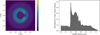 |
Fig. 1 (Left) Example of face-on surface density distribution of dust in a planet’s corotating frame, with a K4-type star located at the origin. The white dot indicates an Earth-like planet placed at the inner boundary of the CHZ. A total of 100 dust particles with a size of 50 μm are used. The resonant ring structure is visible around the planet’s position. The color scale indicates surface density in arbitrary units, with lighter colors corresponding to higher densities. (Right) Azimuthally averaged surface density of dust in arbitrary normalized units, based on the distribution in the left panel. The background disk appears as a nearly constant plateau, while the resonant ring structure shows a density enhancement. |
2.2 Simulation design: Pilot and Main studies
2.2.1 Pilot Study: Setup for evaluating the importance of stellar wind
Based on the ψ parameter, we examined two types of models assuming a radial, non-varying stellar wind within each system. In Model I, we adopted a solar-like stellar wind for all cases, where ψ ∼ 0.3. In Model II, distinct ψ values were applied for cases with different spectral types. For simplicity, we refer to the cases in Model I as those without spectral-type variation in stellar wind, as the ψ value is fixed for all stars. As mentioned in Sect. 1, the spectral types for this study were chosen across F to M-type, motivated by their potential to host more habitable environments (Tuchow & Wright 2022) and their relevance as candidate targets for the LIFE mission (Menti et al. 2024).
For both Model I and Model II, we considered 36 cases each: four types of late-type, main-sequence stars with ages similar to the Sun (F4, G4, K4, and M4), three planetary masses comparable to Earth (Mp = 0.5,1.0, and 2.0 M⊕), and three planetary semimajor axes (ap) within the HZ (inner, middle, and outer boundaries of the CHZ). A stellar age of 4 Gyr was adopted for all simulations, based on the median age of stars known to host small planets (Swastik et al. 2023), as well as the estimated timescale for the emergence of complex life informed by Earth’s evolutionary history (Cuntz 2014; Safonova et al. 2016). This age enters our simulations through the stellar wind prescription used to estimate ψ (see Sect. 3.1), since stellar wind strength depends on stellar rotation and hence age. For F4-type stars, whose main-sequence lifetime is shorter (∼3 Gyr; Choi et al. 2016), the difference between the ψ value for 4 Gyr (∼0.7) and for nominal main-sequence ages of 2-3 Gyr (∼1) is minor when using the same main-sequence stellar parameters (see Appendix B.4 for details) — particularly compared to the much higher values of M-type stars (see Sect. 3.1.1). Therefore, although the input of 4 Gyr age was used for F4-type ψ values for consistency in the simulations, the results were interpreted as representative of mid- to late-main-sequence F4 stars at 2-3 Gyr.
The exact values of ap vary depending on spectral type; for clarity, we denote them as HZin, HZmid, and HZout. We used HZmid rather than the Earth-equivalent insolation distance (EEID), as the latter is nearly identical to HZin. Specific parameter values are given in Table 1, where stellar parameters are taken from the online table of Mamajek, E. E.1 (Pecaut et al. 2012; Pecaut & Mamajek 2013), along with HZ boundaries derived using the method of Kopparapu et al. (2014). These stellar parameters represent average main-sequence values, appropriate for low-mass stars whose main-sequence lifetimes exceed the assumed age. Such stars evolve negligibly over gigayear timescales due to slow hydrogen fusion and convective interiors (Chabrier & Baraffe 1997; Baraffe et al. 2015). Thus, stellar age does not affect parameters other than via ψ in our setup. As noted previously, since the results for F4-type stars can be interpreted as representative of typical or older main-sequence results, the use of these nominal parameters is acceptable (see Appendix B.4).
For each simulation, we used 100 dust particles of fixed size s = 50 μm. The number of particles was selected to balance the computational efficiency of MERCURY6 with the purpose of exploring general trends across different parameters prior to detailed modeling in the main study. The particle size was also chosen as a convenient, computationally efficient baseline to capture general resonant behaviors of bound grains within the typical 1-100 μm range in the Solar System (Grün et al. 1985; Fixsen & Dwek 2002; Kuchner & Holman 2003). Given the limited knowledge of exoplanetary grain size distributions and the pilot study’s focus on isolating the effect of ψ, we adopted this fixed size for all simulations.
The initial semimajor axis of dust was set at about 3 ap, outside the strongest 2:1 and 3:2 MMRs according to Stark & Kuchner (2008). We used initial eccentricities and inclinations of dust released from parent bodies of ep ∼ 0.1 and inclination ip ∼ 5°, considering that the creation of resonant ring structures is dominated by dynamically cold dust, i.e., ed ≤ 0.2 and id ≤ 20° (Stark & Kuchner 2008). We set these fixed initial values of semimajor axis, eccentricity, and inclination for each simulation to simplify the setup and enhance the structures formed by MMRs. Accordingly, our simulations represent the most efficient case in terms of visibility of the resonant structures. The initial values of the longitude of ascending node Ω, argument of pericenter ω, and mean anomaly M were independently drawn from uniform distributions between 0 and 2π for each particle. This ensured that each orbital element was initially random and evenly distributed, and any residual unevenness was quickly erased as the angles became isotropically distributed on relatively short timescales.
Values of stellar parameters and ap.
2.2.2 Main Study: Setup for multi-size dust simulations
To investigate more realistic disk structures, we focused on Model II, incorporating a range of dust sizes (s = 0.1,0.3,1, 3,10, 30,100, and 300 μm) and increasing the number of particles to 5,000 in each size bin. The chosen range covers typical Solar System values (1-100 μm; Sect. 2.2.1) while extending toward both smaller and larger sizes to account for possible variations in other systems.
In Fig. 2, we show the numerically calculated ⟨QPR⟩ and βPR values across the size range based on the optical constants of astronomical silicates (Draine 2003), using Mie theory (prahl 2024). Since βr ≈ βPR (Sect. 2.1.3), the effective blowout sizes are sBO,eff ∼ 1.94 and 0.71 μm for F4 and G4 stars, respectively, while no blowout size exists for K4 and M4 stars. Accordingly, we excluded the 0.1-1 μm sizes for F4 and 0.1-0.3 μm sizes for G4 from the simulations. Further discussion and comparison with previous estimates are provided in Appendix B.1.
The right panel of Fig. 2 shows that the analytical βPR value assuming ⟨QPR⟩ = 1 significantly deviates from the numerical value for 0.1 μm particles while the discrepancy is minor for larger sizes. We therefore adopted ⟨QPR⟩ = 1 for s ≥ 0.3 μm and approximate the 0.1 μm cases using results from larger grains with comparable βPR values (0.3 μm for K4 and 1 μm for M4). This approach is justified because the equation of motion and initial conditions depend directly on βPR rather than on ⟨QPR⟩ (Eq. (5)). For ψ, we retained the assumption QSW/⟨QPR⟩ ≃ 1 across all grain sizes, as the behavior of QSW is analogous to that of ⟨QPR⟩, although the discrepancy becomes large for grains smaller than ∼0.1 μm (Minato et al. 2004; Mann et al. 2006).
The number of particles follows the setup of Stark & Kuchner (2008), who demonstrated that 5000 particles are sufficient for robust evaluation of resonant ring structures by reducing variations in MMR populations across repeated simulation runs. The planetary configuration was fixed (Mp = 1 M⊕, ap = HZmid), with all other parameters identical to the pilot study. This results in a total of 32 cases (27 after excluding the blown-out sizes) across all stellar spectral types. These higher-resolution simulations provide more reliable contrast and density profiles (Stark & Kuchner 2008) and are designed to represent plausible exo-zodi environments around Earth-analog systems. A summary of the parameter definitions and simulation setups for both the pilot and main studies is provided in Appendix A.
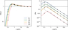 |
Fig. 2 QPR values for grain sizes s ∼ 0.1300 μm (left) and the corresponding βPR values (right ; analogous to Fig. 7 of Rigley & Wyatt 2020). The solid lines show the numerical values for the different stellar spectral types used in this study, while the dashed lines (right panel) indicate the analytical βPR values using QPR = 1 (Eq. (2)). The black dots mark the discrete grain sizes adopted in the main study. The dotted black line (right panel) denotes βPR = 0.5. Sizes above this threshold, corresponding to grains blown out of the system for circular orbits, are marked with cross (×) symbols. The size ∼50 μm used in the pilot study is safely higher than the blowout size and meets the assumption of QPR ∼ 1. |
3 Results
In Sect. 3.1, we present our preliminary findings based on the pilot study approach described in Sect. 2.2.1, using a simplified simulation setup. These results highlight the importance of stellar wind in shaping exozodi resonant structures for various spectral types. Building on these findings, Sect. 3.2 presents the main results based on the multi-size simulations outlined in Sect. 2.2.2, employing more realistic assumptions. We analyze the contrast of resonant rings in Sect. 3.2.1 and examine the optical depth and surface brightness distributions of the exozodis in Sect. 3.2.2.
3.1 Preliminary results based on the pilot study
This pilot study presents the estimated ratio of stellar wind drag to PR drag (ψ) for various spectral types and examines its influence on dust dynamics and resonant structures. The ψ prescription highlights the importance of stellar wind drag, while the simulations quantify its effect on resonant ring contrasts, which cannot be directly inferred from ψ alone (see Sect. 4.3). Based on the estimated ψ values and comparison of two models — with and without stellar spectral-type variation in stellar wind drag — we illustrate the importance of properly incorporating stellar wind in exozodi modeling, particularly around low-mass stars where ψ attains high values.
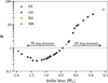 |
Fig. 3 ψ values given by Eqs. (4) and (9) for main-sequence stars of spectral types F4 to M4 at an age of ∼4 Gyr (2-3 Gyr for F-type stars). The four spectral types used in this study are marked in blue, green, yellow, and red, respectively. The dashed line shows ψ = 1, where the stellar wind drag equals the PR drag. |
3.1.1 Estimating stellar wind drag efficiency strength across spectral types
Following Eq. (4), we computed the ψ values for different stellar spectral types. We used the relation from Johnstone et al. (2015, 2021) as input for stellar wind mass-loss rates, applied to main-sequence stars of the spectral types considered in this study:
 (9)
(9)
where R* and P* are the stellar radius and rotation period, respectively. The value of P* was determined using gyrochronology, which depends on stellar effective temperature T* and age. To cover the spectral range (F4-M4) and stellar age (∼4 Gyr) used in this work, we combined results from different gyrochronology studies based on their applicable parameter ranges: for stars with T* ≥ 6280 K (∼F7 and earlier), 6280 K > T* ≥ 4200 K (F7-K6), and 4200 K > T* ≥ 3200 K (K6-M4), we adopted the gyrochronology models of Lu et al. (2024), Mamajek & Hillenbrand (2008), and Dungee et al. (2022), respectively. Although the gyrochrones from Lu et al. (2024) span all spectral types and a broad stellar age range (0.67-14 Gyr), we chose the other two models for lower-mass stars because they generally yield more conservative estimates of ψ — especially for M4-type stars. Additionally, the gyrochrones from Dungee et al. (2022) were constructed specifically for 4 Gyr-old stars, matching the stellar age we assumed. The accuracy of this prescription is further discussed in Sect. 4.1.
Figure 3 presents the resulting ψ values for all main-sequence spectral types in the range of F4 to M4 having an age of 4 Gyr (2-3 Gyr for F-type stars). The results indicate that at these ages of a few gigayears, systems with stellar masses below ∼0.8 M⊙ (approximately K3 type) are more strongly influenced by stellar wind drag than by PR drag. The ψ values for the F4, G4, K4, and M4 spectral types used in this research are approximately 0.73, 0.37, 1.40, and 44, respectively. Notably, the lowest-mass star, M4, exhibits a particularly high value, over an order of magnitude larger than those of earlier types. Using the gyrochrones from Lu et al. (2024) for all spectral types yields an even higher value of ∼127 for M4, whereas the values for the other spectral types remain largely unchanged. While we adopt the more conservative value of ψ ∼ 44 for M4-type stars in our main analysis here, these results demonstrate that M-type systems at even 4 Gyr ages can be dominated by stellar wind drag regardless of the choice of gyrochronology model.
3.1.2 Impact of stellar wind drag: Model I versus Model II
In this subsection, we compare the results of Model I and Model II to evaluate the impact of stellar wind drag on resonant structure formation and model consistency. We examine the prominence of these ring structures, quantified by their contrast relative to the background distribution. Figure 4 shows the contrast values of resonant structures as a function of  , with results presented for different spectral types, planetary masses, and semimajor axes, assuming a fixed dust size.
The contrast values are plotted against  because, according to Stark & Kuchner (2008), contrast depends only on this term and Mp . This expression is derived by the PR drag timescale over the libration timescale for resonance:
 (10)
(10)
where ad ∼ ap since the resonant trapping occurs near the orbit of the planet. Extensions of this formulation that incorporate spectral type and stellar wind effects are introduced later in Sect. 4.3, with the same results plotted against this modified term in Fig. B.2. For clarity and consistency with Stark & Kuchner (2008), we use the original term  when comparing Model I and II. This allows us to isolate the effect of stellar wind drag and assess the differences between the two models under a shared baseline.
For the quantitative calculation of contrast, we adopted CAA,max among the several definitions proposed by Stark & Kuchner (2008), which is the maximum of the azimuthally averaged surface density of the resonant ring relative to the background disk density. To obtain this quantity, we constructed an azimuthally averaged surface density histogram from the 2D dust distribution in the planet’s corotating frame (see Sect. 2.1.5 and Fig. 1). The maximum of this profile was then divided by the average of the nearly constant background density (at r ~ 2-2.6 ap) to derive CAA,max. This choice reflects the fact that azimuthal asymmetries can be significant sources of noise for interferometric observations. For simplicity, we refer to this quantity (CAA,max) as C throughout the paper.
When comparing different spectral types, Fig. 4 reveals that M4-type stars exhibit the highest resonant ring contrasts overall, but their contrast values decrease significantly — from Model I to Model II — by roughly a factor of 2. Other spectral types also show slight reductions, though these are less pronounced than in the case of M4-type. More broadly, the results indicate a general trend of increasing resonant ring contrast with decreasing stellar mass across spectral types, regardless of model. However, using higher ψ values based on an alternative gyrochronology model (see Sect. 3.1.1) could further reduce the contrast for M4-type stars in Model II, shifting the peak contrast toward K-type stars. While we base our analyses on the relatively conservative ψ value throughout this study, the implications of adopting the higher value for M4-type are discussed in Appendix B.3. The findings here highlight two key points: (1) stellar wind drag significantly reduces the prominence of resonant structures around M-type stars, as indicated by the lower contrast of the red points in the right panel of Fig. 4 compared to the left; and (2) resonant ring contrast increases toward lower-mass stars. This confirms our expectation that stellar wind drag across various spectral types should be properly accounted for in exozodi modeling, even at old ages — an important point further discussed in Sects. 4.2 and 4.3.
Across both models, Fig. 4 also demonstrates a general trend of increasing contrast with larger Mp and ap within a given spectral type, consistent with the findings of Stark & Kuchner (2008). Some deviations from this trend are likely due to statistical noise caused by the limited number of particles, as noted by Stark & Kuchner (2008), who showed that simulations with only 100 particles can yield unreliable contrast estimates. To account for this, we conducted internal tests with 5000 particles, which showed consistent trends with the 100-particle simulations, supporting the validity of our model comparison. The agreement between the G-type star results and the contrast fit function from Stark & Kuchner (2008) further supports the consistency of our approach. Deviations from the fit for other spectral types are as expected, as Stark & Kuchner (2008) focused exclusively on solar twins. Improved fits across spectral types, based on the modified parameter that includes spectral type and stellar wind effects, are also shown in Fig. B.2. The detailed fitting functions and their parameter values are introduced in Sect. 4.3, with additional analysis and discussion of their applications in Appendix B.2.
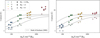 |
Fig. 4 Contrast values from the pilot study, plotted against the |

3.2 Main results from multi-size simulations
The main study expands upon the pilot results by systematically investigating resonant ring contrasts, as well as the spatial distributions of optical depth and thermal surface brightness, across multiple dust sizes and stellar spectral types. Focusing on cases with an Earth-twin planet and properly accounting for spectral-type variation in stellar wind effects, we quantified how dust size, stellar mass, and stellar wind influence the configuration of resonant structures.
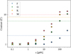 |
Fig. 5 Contrast values from the main study plotted against grain sizes. Cases where s < sBO,eff are shown as cross (×) marks, which overlap with other data points up to 1 μm. The dashed lines indicate the size-combined contrast values of optical depth |

3.2.1 Resonant ring contrasts
Figure 5 shows the contrast values for each particle size from the multi-size simulations. The  term is not used for the plots here to facilitate comparison of contrast across different stellar spectral types for the same dust size. For results plotted with respect to the
  term and the modified expression from Eq. (15); see Fig. B.3.
At a fixed dust size, the contrast increases with decreasing stellar mass, consistent with the key results of the pilot study. For a given stellar type, the contrast also exhibits a general increase with grain size. Larger grains form more pronounced ring structures because they survive longer due to slower inward migration and are more likely to be captured in MMRs (Stark & Kuchner 2008). Smaller grains tend to bypass resonant trapping, and the resulting contrast approaches unity, indicating little to no ring structure. Resonant rings fail to form for grains of s ≲ 1 μm around K and M-type stars, s ≲ 3 μm around G-type stars, and s ≲ 10 μm around F-type stars. We note that the decrease in resonant contrast for Model II, observed in the pilot study when accounting for spectral-type variations in stellar wind (Fig. 4), does not apply to grains in these size ranges. Detailed minimum grain sizes for resonant structure formation, derived from data fits, are given in Appendix B.2.
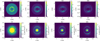 |
Fig. 6 Distributions of optical depth (upper row) and surface brightness (10 μm; lower row) for spectral types F4, G4, K4, and M4, from left to right, assuming a constant τBG ∼ 3 zodis. The star is located at the center of the distributions, and the planet is marked with a white dot to the right of the central star. The spatial scale differs between the upper and lower panels: the optical depth maps show a larger region (∼4 ap) to capture the full disk structure, while the surface brightness provides a zoom-in on a smaller region (∼2 ap) around the planet to emphasize resonant ring structures. All panels have a consistent bin size of ap/50 × ap/50. The color bars vary across spectral types to optimize visualization. For reference, the optical depth at r ∼ 2 ap is τBG ≈ 2.1 × 10⁻⁷ for all spectral types. The inner regions of the surface brightness maps are saturated above the ring maximum and excluded within the sublimation distance. The spatial scale also varies with spectral type, with lower-mass stars having more compact configurations. These results correspond to Model II only, as they are from the main study. Note that we derive our results from grain sizes of 0.1-300 μm and may differ if larger grains are included (see Sect. 4.5). |
3.2.2 Optical depth and surface brightness distributions
The vertical geometrical optical depth, τ, referred to simply as optical depth for clarity, was calculated from the surface density distributions of each grain size. It accounts for the combined contributions of all dust sizes, considering their total crosssections. Figure 6 shows the distributions of exozodi optical depth and the corresponding thermal emission for F4, G4, K4, and M4 spectral types. Resonant structures were formed in all cases. In particular, larger dust grains contribute more significantly to these structures, as their dynamics are more strongly governed by gravity, as explained in Sect. 3.2.1. As a result, the optical depth distribution is primarily shaped by the largest grains, though it is diluted by the abundance of smaller particles produced by collisional cascade (Eq. (11)) and retained due to the small blowout sizes of late-type stars (Fig. B.1). This is consistent with the findings of Stark & Kuchner (2008).
The effect of this dilution can be seen by comparing the size-combined contrast with the contrast from single-sized exozodis composed of only the largest grains. The optical depth contrast, ⟨Cτ⟩, represents the contrast of the size-combined resonant ring and is calculated directly from the azimuthally averaged histograms of the optical depth distributions. It follows the same methodology as CAA,max (Sect. 3.1.2), which measures the contrast for single-grain-size distributions; however, ⟨Cτ⟩ incorporates the contributions of all grain sizes, naturally accounting for the dilution effect from smaller grains. The original semi-analytical definition from Stark & Kuchner (2008) is provided in Appendix B.2. The resulting ⟨Cτ⟩ values are 1.95, 5.98, 8.07, and 9.85 for F4, G4, K4, and M4, respectively, with modest (≲20%) numerical variations that do not affect the main results. Each of these values is lower than the estimate based solely on the largest grains, as marked in Fig. 5. Overall, ⟨Cτ⟩ increases with decreasing stellar mass, consistent with trends observed in previous single-size cases. This confirms that resonant rings become more prominent around lower-mass stars, even when extended to more realistic multi-size dust distributions.
The detailed calculation of optical depth was performed under the assumption that dust production follows a collisional cascade (Dohnanyi 1969),
 (11)
(11)
with particles not undergoing further collisions after release from their parent bodies (Stark & Kuchner 2008). Results from individual simulations were combined into composite models weighted by this size distribution. This approach is valid up to the critical grain size where the collisional timescale becomes comparable to the migration timescale (Kuchner & Stark 2010) for a given dust level. Bearing this limitation in mind, the applicability and caveats of our simulation results are further discussed in Sect. 4.5.
The optical depth was then computed as
 (12)
(12)
where n(s) is the surface density of particles with size s, N(s) is the number of dust particles in a given area ΔA, s0 is the reference size (1 μm), N0 is the normalization number of particles at the reference size, and Δs is the bin width in particle size, corresponding to a constant logarithmic interval in s. The value N(s) was calculated considering the different output time steps of the simulations, and ΔA corresponds to the projected area of each simulation grid cell. The value of N0 is determined by the dust production rate of the parent body, which can vary randomly between systems. We scaled N0 according to a specified background optical depth (at r ~ 2-2.6 ap) in zodis, where 1 zodi corresponds to the optical depth of the zodiacal dust of the Solar System at 1 au, ∼7.12 × 10⁻⁸ (Kelsall et al. 1998). For the nominal background level, we adopted τBG ~ 3 zodis for all stars, which corresponds to the median best-fit value inferred from the Hunt for Observable Signatures of Terrestrial Systems (HOSTS) survey population modeling, independent of spectral type and age (Ertel et al. 2020). Although M-type stars were not included in the survey, we assumed the same value due to the lack of confirmed observational constraints (see Sects. 4.2 and 4.3 for details). For reference, the 95% confidence upper limit of 27 zodis reported by HOSTS is also considered in our comparison of collision and migration timescales (Sect. 4.5) to assess the validity of our results for dustier systems.
Because of their higher ring contrast, lower-mass stars exhibit more optically thick resonant structures for the same background level in the optical depth maps (upper row of Fig. 6). The surface brightness (Iλ) maps (lower row) were derived from the optical depth distributions by
 (13)
(13)
where (x, y) is the position in astrocentric coordinates, with the planet located at (ap, 0). The value Bλ denotes the Planck function, and T is the equilibrium temperature at that location, assuming that the dust behaves as a perfect blackbody. A nominal MIR wavelength λ = 10 μm was used, within the LIFE wavelength coverage of 4-18.5 μm (Dannert et al. 2022).
To show the intrinsic emission morphology of each disk, the surface brightness maps presented in Fig. 6 display emission down to the dust sublimation distance. This allows the bright inner regions originating from hot dust located close to the star to be represented, saturated above the maximum value in the ring. Detailed analyses of the surface brightness maps are presented in Sect. 4.4, where we focus on the resonant structures rather than these central regions. Overall, the optical depth and surface brightness maps presented here characterize exozodi distributions around late-type stars, incorporating stellar wind drag and the resonant structures induced by exo-Earths.
4 Discussion
This section discusses the broader implications of our results for the modeling of exozodi distributions, focusing on the influence of stellar wind drag, spectral type, and stellar age on resonant structures and planet detectability. We first evaluate the accuracy and the age dependence of the adopted ψ prescription (Sect. 4.1) and then examine how stellar wind drag influences dust dynamics and ring contrasts, with particular emphasis on M-type stars (Sect. 4.2). We then explain how the contrast and optical depth vary with spectral type (Sect. 4.3) and explore their observational impact by analyzing asymmetric surface brightness features and flux per beam, which could be confused with planetary signals (Sect. 4.4). The validity of the collisionless assumption is lastly considered, along with other model limitations (Sect. 4.5). Additional analyses and caveats are briefly introduced here, with detailed discussions provided in Appendix B.
4.1 Reliability and age dependence of the ψ prescription
The ψ values in this study were estimated via a stepwise prescription: stellar rotation periods (P*) were derived from gyrochronology models based on T* and age, mass-loss rates (Ṁ*) from Eq. (9), and ψ from Eq. (4). Uncertainties mainly stem from P* and Ṁ*, while errors in basic stellar parameters and the functional form of Eq. (4) were neglected.
We adopted three gyrochronology models — Lu et al. (2024), Mamajek & Hillenbrand (2008), and Dungee et al. (2022) — applied sequentially from F4 to M4 stars (Sect. 3.1.1). The Lu et al. (2024) relation provides consistent calibration across the full spectral range up to ∼14 Gyr, with typical P* uncertainties of ∼10%. For G-K stars, Mamajek & Hillenbrand (2008) has minimum P* uncertainties of ∼0.12 days. Dungee et al. (2022) yields results consistent with Lu et al. (2024) with similar uncertainties but offers a more conservative calibration of ψ for M-type stars, exclusive for 4 Gyr-old ages. The ∼10% uncertainty reflects the precision of individual P* measurements, supported by cross-survey validation (Lu et al. 2024) and injection-recovery tests (Dungee et al. 2022).
Mass-loss rates follow Johnstone et al. (2015, 2021), which are constrained for 0.1-1.2 M⊙ main-sequence stars via rotational evolution models tied to observed cluster rotation periods, but are less certain for fully convective M-dwarfs. The exponents in the scaling with P* and M* have typical uncertainties of order a few tens of percent, reflecting the fitting uncertainties to the model. Inherent limitations and assumptions of the wind models may introduce additional uncertainties that are more difficult to quantify.
The propagated uncertainties in ψ (Fig. 7) are the largest for F4 and M4 stars, mainly reflecting limited observational constraints and magnetic dynamo variability in fully convective stars. Nevertheless, the overall trend of increasing ψ toward late K-M types is consistent across all models. Across the varying ψ values from different gyrochronology models, we adopted the conservative estimates for each stellar type (Fig. 3). The particularly large ψ value for M4-type stars primarily arises from their low stellar luminosities: at 4 Gyr, Fig. 7 shows that an M4 star has a long rotation period of ∼151 days inferred from the observed slow-rotator sequence in M67 (Dungee et al. 2022) and a modest stellar mass-loss rate of ∼1.06 M⊙, comparable to G-K stars. However, its extremely low luminosity (∼0.0072 L⊙; Table 1) greatly enhances the importance of stellar wind drag relative to radiation, producing the higher ψ via Eq. (4).
To assess age dependence, we recomputed ψ at 1, 4, and 10 Gyr using the Lu et al. (2024) gyrochrones (Fig. 8). Younger systems show systematically higher ψ across all spectral types, with most exceeding unity and M4 stars reaching ∼343 at 1 Gyr compared to ∼127 at 4 Gyr. While we do not extend our analysis to even younger ages due to gyrochronology limits, the increasing dominance of stellar wind drag with decreasing age is consistent with previous findings (e.g., Najita & Kenyon 2023). The K2-type star e Eridani, with an age of ≲1 Gyr, has a value of ψ ∼ 28 derived from observed mass-loss rates (Reidemeister et al. 2011), higher than the value (∼2) for 1 Gyr in Fig. 8. Likewise, the M0-type star AU Mic at ∼15 Myr is estimated to have ψ values of a few thousand (Plavchan et al. 2005; see Appendix B.1), further illustrating the expected steep age dependence. At older ages (∼10 Gyr), ψ decreases but remains above unity for K-M stars that remain on the main sequence, implying that stellar wind drag can still be relevant even in such old, low-mass systems.
Overall, this prescription provides a practical means to estimate stellar wind drag strength for main-sequence stars between F4 and M4 types and ages of ∼0.7-14 Gyr. Outside this range, Ṁ* should be derived from direct observational methods.
Despite the underlying uncertainties, the combined stellar-type and age trends of ψ are physically supported and justify the ψ values adopted in our simulations.
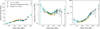 |
Fig. 7 Stellar rotation period (P*, left), mass-loss rate (Ṁ*, middle), and ψ (right) for main-sequence stars of spectral types F4-M4 at age 4 Gyr (2-3 Gyr for F-type). Different symbols and colors show results from the three gyrochronology models, with approximate uncertainties. |
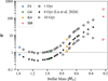 |
Fig. 8 ψ values given by Eqs. (4) and (9) for main-sequence stars of spectral types F4-M4 at an age of 1 Gyr (empty circles), 4 Gyr (2-3 Gyr for F-type stars; filled circles), and 10 Gyr (empty triangles) using gyrochrones from Lu et al. (2024). For 10 Gyr, only values for stars with masses below ∼0.8 M⊙ are shown, as more massive stars have evolved off the main sequence by that age (Choi et al. 2016). The 4 Gyr results are almost identical to those in Fig. 3, except for the larger M4 value due to the change in the gyrochronology model. |
4.2 Influence of stellar wind drag on debris disk structures
The ψ values used in this study (Fig. 3) indicate that stellar wind drag can substantially influence dust dynamics around K-M-type stars, even at gigayear ages comparable to that of the Solar System. This complements earlier studies (e.g., Stark & Kuchner 2008; Defrère et al. 2010), which primarily considered PR drag as the main dust migration mechanism and used a constant solar wind value of ψ ∼ 0.3. In particular, the high value of ψ ∼ 44 for the M4-type star demonstrates that stellar wind drag can remain dynamically important over a wide range of evolutionary stages. This finding builds on the age-dependent trends discussed in Sect. 4.1, showing that while the stellar wind dominance inferred for young early K-type stars (e.g., e Eridani; Reidemeister et al. 2011) weakens with age, late K to M-type stars can retain strong drag effects throughout their main-sequence lifetimes.
The high ψ values underscore the importance of incorporating stellar wind drag into models of dust distributions around old, low-mass stars — a significance further supported by our pilot study comparing ring contrast between the two models (see Sect. 3.1.2). Since βt increases with ψ, a higher value of ψ results in a shorter migration timescale, as can be inferred from Sect. 2.1.2 (Mann et al. 2006; Plavchan et al. 2005). This faster migration reduces the probability of resonant trapping, thereby lowering the resulting ring contrast. Consequently, an increase in the ψ value yields weaker resonant ring structures (see Eq. (14)), as illustrated most clearly by the contrast change for the M-type star between Model I and Model II (Fig. 4). The contrasts for higher-mass stars exhibit smaller variations since the differences in their respective ψ values between the two models are less pronounced.
This reduction in ring contrast may have important observational implications. Using constant solar wind drag values regardless of spectral-type variation can cause an overestimation of the resonant ring optical depth by nearly a factor of 2 in the M4-type case (see Sect. 3.1.2). This highlights the need to revisit observational strategies for M-dwarfs with updated models that properly account for stellar wind. Including spectral-type-dependent stellar wind drag can alter expectations for the detectability of exozodiacal structures around M-type stars, potentially broadening the range of viable targets for general exo-Earth searches. Accurate modeling of stellar wind is thus essential for realistic exozodi predictions around M-type stars.
Similarly, in smooth disks without resonant structures (e.g., Kennedy et al. 2015), accounting for stellar wind could lower noise from dust when replenishment is limited, rather than maintaining a fixed background optical depth. In such cases, stellar wind lowers optical depths by speeding up dust migration (τBG ∝ tmig ∝ (1 + ψ)−1). This implication aligns with the analytical work of Plavchan et al. (2005), who attributed the lack of infrared excess detections around M-dwarfs aged ten to hundreds of megayears to the dominance of stellar wind drag. To explain this, they constructed a debris disk model in which collisional dust production is balanced by removal via stellar wind and PR drag. Unlike our model, which assumes continuous dust replenishment, their model includes gradual depletion of planetesimal reservoirs over time. Under such conditions, strong stellar wind drag rapidly removes dust, consistent with our study where higher ψ values correspond to shorter effective migration timescales. Najita & Kenyon (2023) reached similar conclusions for young (<1 Myr) Sun-like systems undergoing terrestrial planet formation, under the assumption of strong stellar wind drag.
Further support for stellar wind-driven dust removal may come from the lack of warm excess in the AKARI 18 μm survey (Fujiwara et al. 2013), although current surveys targeting colder dust around M-dwarfs (Cronin-Coltsmann et al. 2023; Lestrade et al. 2025) suggest that such non-detections are a product of observational bias due to limited sensitivity. The studies by Morey & Lestrade (2014) and Binks (2016) point to both possibilities — the dearth of dust around M-dwarfs resulting from either stellar wind drag removal or observational limitations. While further data with improved sensitivity are needed for confirmation, the estimations of ψ suggest that in systems with limited dust replenishment, old M-type stars are likely to lack dust due to rapid inward migration. Our results thus extend the work of Plavchan et al. (2005) and Najita & Kenyon (2023) by explicitly presenting estimates of stellar wind drag strengths across spectral types from F to M, focusing on older systems. However, predictions may differ when assuming continuous dust production and the presence of resonant structures, as considered in our model (see Sect. 4.3).
4.3 Stellar-type dependence of resonant structures
Despite the influence of stellar wind, our results show that the ring contrast increases for lower-mass stars, with M-type stars exhibiting the highest values (Fig. 4). This trend arises because the reduction in M* has a stronger influence than the increase in ψ in determining the contrast. The contrast can be described by extending the semi-analytical functional form of Eq. (4) from Stark & Kuchner (2008), following the approach of Wyatt (2003) to fit an empirical function with power-law dependencies on the relevant physical parameters:
![Mathematical equation: C = 1 + p_1 \left[ 1 + \left( \frac{p_2}{a_\text{p}^{1/2} \left[ \beta_\text{PR} \left(1+\psi\right) \right]^{-1} M_\ast^{-1/2}} \right)^{p_3} \right]^{-1},](/articles/aa/full_html/2026/06/aa56764-25/aa56764-25-eq22.png) (14)
(14)
where  , with Mp and M* in units of M⊕ and M⊙, respectively. This form shows that the contrast depends on Mp/M* and the modified term
 ![Mathematical equation: $a_\text{p}^{1/2} \left[ \beta_\text{PR} \left(1+\psi\right) \right]^{-1} M_\ast^{-1/2} $](/articles/aa/full_html/2026/06/aa56764-25/aa56764-25-eq24.png) , expanding from the original parameters from Stark & Kuchner (2008) (see Sect. 3.1.2). The latter term is derived similarly as Eq. (10) (Wyatt 2003; Kuchner 2003; Shannon et al. 2015):
, expanding from the original parameters from Stark & Kuchner (2008) (see Sect. 3.1.2). The latter term is derived similarly as Eq. (10) (Wyatt 2003; Kuchner 2003; Shannon et al. 2015):
![Mathematical equation: \frac{t_\text{mig}}{t_\text{lib}} \propto \frac{a_\text{d}^2/\left( \beta_\text{t} M_\ast \right)}{a_\text{p}^{3/2} M_\ast^{-1/2}} \propto a_\text{p}^{1/2} \left[ \beta_\text{PR} \left(1+\psi\right) \right]^{-1} M_\ast^{-1/2},](/articles/aa/full_html/2026/06/aa56764-25/aa56764-25-eq25.png) (15)
(15)
where the additional drag due to stellar wind is included in the effective migration timescale (see Eq. (8)). The best-fit parameters pi are
 (16)
(16)
where the coefficients were obtained through nonlinear leastsquares fit to all simulated contrast values across different stellar types, planetary masses, and dust sizes from both the pilot and main study. Most parameters are constrained to 10-20%, though the exponents p1,2 and p3,2 have larger uncertainties (∼50%). These values offer a first-order estimation of the contrast rather than an exact analytical solution, with further discussion provided in Appendix B.2.
For fixed values of Mp and s, the denominator term  of Eq. (14) scales as M*−2.125 (1 + ψ)−1, using
  ,
,  , and L* ∝ M*3.5 (see Sect. 2.1.1 and Eq. (2)). Although ψ increases up to ∼44 for M4-type stars, this increase is insufficient to offset the stronger effect of decreasing M*. The parameters in the contrast function (Eq. (16)) vary in a way that further enhances the contrast as M* decreases, with p1 increasing and p2, p3 decreasing. As a result, the resonant ring contrast overall increases with decreasing stellar mass. This relation can also be approximately estimated from the original term
  , although a more precise derivation requires extra M* terms and the inclusion of ψ as done here. When ignoring ψ, this trend can also be understood intuitively from the definition of βPR, where a lower stellar mass yields a smaller βPR (Eq. (2)). This implies that dust particles in systems with lower-mass stars remain more gravitationally bound and are more likely to be trapped in MMRs, assuming a fixed dust size. Therefore, for the same level of background exozodi, lower-mass stars are expected to host more optically thick resonant structures — though not to the extent predicted by models without spectral-type variation in ψ (e.g., Model I). As mentioned in Sect. 3.1.2, a possible inversion of this trend between K and M-type due to even higher ψ values for M4-type is discussed in Appendix B.3.
Since the maximum optical depths appear as part of the asymmetric structure around the inner edge of the resonant ring as seen in the optical depth distributions, the azimuthally averaged maximum contrast C serves as a useful proxy for roughly estimating the peak exozodi signal most threatening to planet detection. Using the size-combined contrast values, we can approximate the strongest contamination level as τBG ∙ ⟨Cτ⟩ (see Sect. 3.2.2 for definition of ⟨Cτ⟩), offering a crude estimate of the exozodi noise. For instance, assuming a fixed background level of 3 zodis, the resulting resonant ring optical depths may reach up to 3 ∙ 1 ∙95 ≈ 6 zodis for F-type stars, 3 · 5∙98 ≈ 18 zodis for G-type, 3 · 8∙07 ≈ 24 zodis for K-type, and 3 · 9∙85 ≈ 30 zodis for M-type stars (Sect. 3.2.2).
Consequently, the optical depth of resonant structures would be higher for systems with stellar masses lower than the Sun, and vice versa for systems with higher stellar masses, compared to the results expected from the resonant models of Stark & Kuchner (2008). This strengthens the importance for considering different spectral types for resonant structure modeling, rather than relying solely on solar twin assumptions as done in previous studies (e.g., Defrère et al. 2010; Stark et al. 2015; Currie et al. 2023). The increase in optical depth up to a factor of ∼2-10 relative to the background level (see Sect. 3.2.2) also suggests the need to include resonant structures in exo-zodi models, when aiming to utilize it for estimating exoplanet observations.
While our models predict systematically higher optical depths for resonant structures around lower-mass stars, current observational surveys of warm dust do not yet reveal a clear dependence on stellar type. For instance, the HOSTS survey with LBTI (Ertel et al. 2020) did not find a statistically significant increase in exozodi levels toward low-mass stars. This apparent discrepancy likely stems from sample limitations, which included only A to K-type stars and mostly lacked known planets in their HZs, with τ Ceti being an exception (Tuomi et al. 2013). Recent work by Huang et al. (2025) using the Wide-field Infrared Survey Explorer (WISE; Wright et al. 2010), found that extreme warm-dust excesses (>21%) occur in fewer than 1% of M-type stars, consistent with previous results for FGK stars (Kennedy & Wyatt 2013). They emphasize that current facilities such as WISE and LBTI lack the sensitivity to detect fainter exozodis — such as those considered in this work — leaving most LIFE-resolvable exo-Earth targets unconstrained. Similarly, these survey results do not directly constrain planet-associated dust structures, limiting their relevance to our resonant model predictions.
Rather than contradicting our findings, these observational gaps address the need for dedicated studies of systems with known planets in the HZ. Our models suggest that, in such systems, resonant structures induced by planets could result in more prevalent warm exozodis around lower-mass (K and M-type) stars, potentially at levels below the sensitivity of current surveys. Thus, while existing data do not constrain the low-density disks relevant to our study, our results may help inform expectations for future observations targeting faint exozodis in the vicinity of planetary orbits.
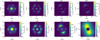 |
Fig. 9 Asymmetric surface brightness (10 μm; upper row), and corresponding flux per beam relative to the planet flux Fp (lower row), following the format of Fig. 6. The inner regions are saturated above the ring maximum, and all maps are shown within a spatial scale of ∼2 ap. The asymmetric surface brightness maps here follow the approach of Fig. 11 in Defrère et al. (2010). The area within the IWA is masked in the flux per beam maps, assuming d = 10 pc and B = 100 m. For reference, the beam FWHM (λ/B ≈ 0.2 au) is about twice the diameter of the IWA mask. |
4.4 Exozodi brightness distributions across spectral types
While contrast-based estimates offer a useful diagnostic of resonant ring significance, the simulated optical depth maps presented in this work (Fig. 6) provide spatially resolved input for observational simulations, such as LIFEsim. These maps enable a more comprehensive evaluation of how exozodis affect the detectability of planets.
To explore asymmetric structures, which can be critical sources of confusion with planetary signals, we computed asymmetric surface brightness distributions by subtracting the brightness of the centrally symmetric counterpart from each pixel of the original surface brightness map and taking the absolute value of the residuals, following the method illustrated in Fig. 11 of Defrère et al. (2010):
 (17)
(17)
where I(x, y) is the surface brightness at each pixel and I(-x, -y) is that of the pixel symmetric with respect to the star. The results are given in the upper row of Fig. 9, at the same high resolution as the lower row of Fig. 6 to show the morphology. Although some central residuals appear in the asymmetric maps due to imperfect numerical cancellation, they are nearly symmetric and will likely contribute to shot noise under interferometric observations, rather than representing signals that could mimic planetary detections. For all types of stars, the central regions where the surface brightness is greater than that in the resonant ring are saturated to highlight the relevant asymmetric structures. Throughout this section, ring surface brightness and flux refer to local quantities in the resonant ring region, not integrated or background-subtracted values.
To approximately compare the asymmetric flux per resolution element with the planetary flux in interferometric observations, we present the flux per beam in the lower row of Fig. 9. We assumed a fixed distance of d = 10 pc for all spectral types and adopted the nominal observation parameters for the LIFE instrument (Dannert et al. 2022; Carrión-González et al. 2023): a mirror diameter of D = 2 m, nulling baseline B = 10-100 m, and a field of view of ∼ λ/D, safely larger than the scale of 2 ap.
We fixed the nulling baseline length to B = 100 m to reflect the most favorable observing configuration for small angular separations, which yields a typical inner working angle (IWA) of ∼0.0052″ at λ = 10 μm (Cesario et al. 2024). The angular distances of the planets at a distance of 10 pc are 0.25, 0.13, 0.064, and 0.013″ for systems with F4, G4, K4, and M4 stars, respectively, all of which lie outside the nominal IWA. To obtain the flux per beam, we convolved the asymmetric surface brightness maps with a fixed Gaussian beam of full width at half maximum (FWHM) ~λ/B ~ 0.02″ and multiplied by the corresponding beam solid angle. The asymmetric flux per beam is presented relative to the emission from the planet, where we assumed planetary thermal equilibrium with albedo A ≈ 0.3 similar to Earth (Charbonneau et al. 2005). This procedure is not intended to simulate the detailed response of a nulling interferometer, but rather to provide a rough estimate of the signal expected at a comparable resolution.
Focusing on the resonant ring region, the asymmetric surface brightness maps in Fig. 9 reveal structures that could be confused with the planetary signal. The maximum surface brightness of these asymmetric ring structures is compared across stellar types in Fig. 10. As discussed in Sect. 4.3, lower stellar mass increases the contrast and thus the optical depth of the resonant ring for a fixed background level. The maximum surface brightness of the ring (Fig. 6) follows this trend of increasing optical depth, as the equilibrium temperature is similar across spectral types because the ring forms near the HZ (see Eq. (13)). Since the asymmetric structures mainly originate from the resonant ring, the maximum asymmetric surface brightness likewise increases toward low-mass stars.
Figure 10 shows that the maximum asymmetric flux per beam follows a similar trend to that of the surface brightness but drops for M-type stars, with K-type stars yielding the strongest signal relative to the planetary thermal emission. This trend arises from the high flux dilution for M-type stars, because the fixed beam covers a larger fraction of the compact system. The competing effects of increasing surface brightness and flux dilution from the decreasing physical scale cause a peak in the resonant ring flux per beam for K-type stars, rather than a monotonic increase toward lower stellar masses. This behavior reflects the fundamental interplay between stellar gravity and radiation in shaping the resonant structures. Dust grains around lower-mass stars are more gravitationally bound (as discussed in Sect. 4.3), which enhances resonant trapping and boosts the resulting ring contrast, optical depth, and surface brightness. At the same time, the spatial extent of the resonant structure shrinks since lower-mass stars emit less radiation and have closer-in HZs. The K-type stars represent a balance point — gravity dominates enough to enable strong resonant structures, while radiation remains sufficient to avoid the tight spatial compactness that limits flux per beam when observing M-type systems. When using shorter or longer baselines, the flux per beam for lower-mass stars is expected to decrease or increase due to the corresponding change in beam size, deviating from the results presented here.
Although Quanz et al. (2022) concluded that exozodi resonant structures are unlikely to pose a significant obstacle to planet detection, their analysis relied on the studies of Defrère et al. (2010), which are limited to solar twin systems. Our results show that the maximum asymmetric flux per beam compared to the planetary flux for a K-type star can be nearly twice that of a G-type (Fig. 10), emphasizing the need for further examination of stars beyond solar analogs. These results suggest that resonant structures should be considered across late-type stars (F4-M4) when modeling exozodis for interferometric observations. While this conclusion is based on a relatively low background level of 3 zodis, implications for higher background exozodi levels are discussed in Sect. 4.5.
The asymmetric surface brightness map for the G4-type star closely resembles that shown in Fig. 11 of Defrère et al. (2010), as both are based on the work of Stark & Kuchner (2008). However, our simulations continue to track dust inward to the sublimation zone, whereas Stark & Kuchner (2008) truncate the disk at half the planet’s position. While Defrère et al. (2010) note that this absent inner disk component is likely insignificant due to its expected central symmetry — an assumption our simulations confirm — our results indicate that including this region can still improve shot noise estimates, particularly given the high levels of brightness found in the area. Although strict conclusions regarding the modulated signal and cross-correlation for interferometry will require further analysis, these results provide valuable direction for refining future studies, particularly for the LIFE mission.
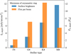 |
Fig. 10 Maximum value of the asymmetric surface brightness of resonant ring at 10 μm (blue, left axis) and the flux per beam (orange, right axis) for each spectral type, assuming a constant background level of ∼3 zodis, grain sizes of 0.1-300 μm, nulling baseline B = 100 m, and distance d = 10 pc. Higher dust levels or the inclusion of larger grains may alter the brightness and fluxes (see Sect. 4.5). Note that the two values are not in scale. |
4.5 Collisional effects and model limitations
While this work represents a scenario where the impact of resonant structures is maximized, introducing more realistic factors such as dust grain collisions, inclusion of dust with more dynamically hot initial conditions, or the presence of additional planets, would likely reduce the contrast and ease the observational constraints (Stark & Kuchner 2008; Stark & Kuchner 2009; Kuchner & Stark 2010; Defrère et al. 2010). To evaluate the validity of our results neglecting particle collisions, we compared the timescales for effective migration by PR and stellar wind drag against the collisional timescale. The effective migration timescale for a grain at a distance a from the star is given by
 (18)
(18)
using Eqs. (2) and (8). Following the methods of Najita & Kenyon (2023) and adapting their Eq. (6), the collisional timescale is
 (19)
(19)
assuming collisions between grains of size s and larger particles, in an exozodi with face-on optical depth τ. The value P represents the orbital period of the particle. If sBO,eff does not exist, the smallest size in the system is used instead. Equation (19) assumes a standard s−3.5 size distribution, in which the optical depth is dominated by grains of size sBO,eff. If drag modifies the size distribution and reduces the contribution of small grains, the collisional timescale would increase, making this a conservative estimate for the comparison that follows.
The collisional timescale defined above differs from the mean collisional timescale  (Wyatt 2003; Kuchner & Stark 2010), which includes impacts with grains of all sizes and therefore typically yields shorter timescales. Such mean timescales are commonly implemented in classical estimates of the zodiacal cloud (e.g., Grün et al. 1985), but more recent studies suggest that actual collisional lifetimes may be longer than these classical estimates by tens of times (e.g., Nesvornÿ et al. 2011; Soja et al. 2019; Pokornÿ et al. 2024), with discrepancies across the literature. In light of this uncertainty, we adopted Eq. (19), which is consistent with our physical framework in terms of the underlying size-dependent collisional cascade and catastrophic disruption. This prescription can yield collisional timescales that are up to hundreds of times longer than ⟨tcoll⟩, depending on the size regime and stellar spectral type. The implications of adopting the more conservative ⟨tcoll⟩ are nevertheless briefly examined (see Appendix B.5) to illustrate the systematic uncertainty associated with the choice of collisional timescale. Accordingly, the results presented in this section should be interpreted as first-order estimates within this framework, with the normalization of the collisional timescale remaining uncertain at the order-of-magnitude level across different studies and prescriptions.
Following Fig. 3 of Najita & Kenyon (2023), tmig and tcoll are shown in Fig. 11 for a smooth disk without planetary perturbations, evaluated at ∼ap (HZmid) for grain sizes of 0.1-1000 μm. Across all grain sizes and stellar types (FGKM), tcoll > tmig even for disks up to a few hundred zodis, confirming that the collisionless assumption is valid for the nominal 3 zodis and the 27 zodis upper limit reported by HOSTS. This likely produces a steady-state size distribution ∝ s−2.5 in the absence of planetary perturbations, as smaller grains are preferentially removed by drag forces (Stark & Kuchner 2008). Stellar wind-driven migration dominates over collisions particularly for M-type stars, extending the findings of Plavchan et al. (2005) to gigayear-age systems. While dust around GJ 581 (2-8 Gyr, M3) is known to be more collisionally influenced (Lestrade et al. 2012), this applies to its cold disk at ∼25 au (∼1000 zodis), not the lower levels of closer-in warm exozodis considered here.
For the densest regions, we compared the resonant trapping timescale tres (total survival time minus tmig) with tcoll at the azimuthal maximum of ring τBG ∙ ⟨Cτ⟩ (Fig. 12). At τBG = 3 zodis, tres ≲ tcoll across all grains producing resonant structures, confirming the collisionless assumption. For 300 μm grains (GKM), tres approaches tcoll, defining the critical size up to which the largest grains dominate the ring (Kuchner & Stark 2010). F-type stars could support centimeter-sized or larger grains, potentially producing resonant rings with contrasts comparable to M-type stars (estimated from Fig. 5 and Eq. (14)). This may result in F-type stars exhibiting the highest ring brightness due to higher optical depths (Sect. 4.4). While this scenario is unlikely if exozodis share the typical size range of 1-100 μm of zodiacal dust, we caution against directly applying our results to dust populations extending beyond 300 μm.
At higher background levels (τBG = 27 zodis), collisions become relevant for grains ≳100 μm (G-type) or ≳50 μm (K and M-type). Pilot study results for s ~ 50 μm remain valid, while main study results for 100-300 μm may not. Under these conditions, ⟨Cτ⟩ is expected to be lower than in Fig. 5: G stars would follow ∼100 μm contrasts (∼6), K and M stars ∼50 μm (∼5-6). For F stars, the collisionless assumption still holds, allowing grains up to roughly 1000 μm and producing comparable contrasts. Overall, at higher dust levels and broader size distributions, we tentatively expect similar resonant ring contrasts and surface brightness across FGKM stars.
We also note that adopting the mean collisional timescale ⟨tcoll⟩ would imply stronger collisional effects and a more restricted regime of validity, warranting caution for grain sizes typically beyond a few tens of micrometers and at higher dust levels. However, the relative trend of stronger resonant ring structures around lower-mass stars holds for the nominal case of τBG = 3 zodis (see Appendix B.5).
While our simulations assume face-on viewing geometry, the results from Defrère et al. (2010) have shown that exozodiacal noise increases with system inclination. Thus, more conservative estimates would be necessary regardless of spectral type when dealing with highly inclined targets (Quanz et al. 2022). In light of these limitations, the models presented in this work could be further improved by incorporating particle collisions and extending the analysis to inclined systems. Future work may also focus on more rigorously assessing the influence of resonant structures on the detection of exo-Earths around different spectral types using nulling interferometry, by deriving modulated signals and applying cross-correlation techniques based on the optical depth and surface brightness distributions obtained here. Modeling the scattered-light flux from our optical depth maps would also benefit coronagraphic exoplanet imaging missions such as HWO.
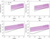 |
Fig. 11 Comparison of timescales for effective migration driven by PR and stellar wind drags (solid black lines), evaluated at an age of 4 Gyr (2-3 Gyr for F-type), with the collisional timescale corresponding to the optical depths τBG = 3 and 27 zodis referenced from the HOSTS survey (dashed purple lines; see Sects. 3.2.2 and 4.3). The comparison is made near the position of the planet ∼ap (HZmid). Collisional timescales for a range of face-on optical depths, τ = 1-1000 zodis, are also shown as a purple band (top to bottom). Results are shown for each stellar spectral type as a function of grain size over 0.1-1000 μm, restricted to s ≥ sBO,eff and adapted from Fig. 3 of Najita & Kenyon (2023). |
4.6 Additional analyses and caveats
To aid the interpretation and application of our results, we highlight several underlying assumptions and extended analyses, detailed in the appendices. These include discussion on the effective blowout size across spectral types (Appendix B.1), semi-analytical contrast functions for efficiently estimating resonant ring strengths across spectral types (Appendix B.2), and the impact of alternative gyrochronology models on ψ and resonant structures (Appendix B.3).
We also discuss further caveats of the study, regarding assumptions related to stellar evolution, particularly for F-type stars (Appendix B.4). Along with the limitations introduced in Sect. 4.5, such factors should be considered when applying our results to observational predictions or interpreting resonant structures in exozodi modeling. Acknowledging these considerations will help guide more comprehensive follow-up studies and ensure robust application to future interferometric missions.
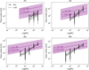 |
Fig. 12 Comparison of timescales for resonant trapping from simulation data (black dots) with the median values (solid black lines) and 1σ uncertainties (gray bands), against the collisional timescale corresponding to the maximum resonant ring optical depth of τBG ∙ ⟨Cτ⟩ (dashed purple lines). For each ⟨Cτ⟩ value of ∼2, 6, 8, and 10 for F, G, K, and M-types stars, τBG values of 3 (upper dashed line) and 27 zodis (lower dashed line) are examined (see Sect. 3.2.2). Other plotting conventions are identical to those in Fig. 11. |
5 Summary and conclusion
We simulated dust in F, G, K, M-type systems, modeling resonant rings around exo-Earths in the HZ and extending the work of Stark & Kuchner (2008). Stellar wind plays a significant role in shaping dust dynamics, dominating over PR drag in M-type stars (ψ ∼ 44) even at an old age of a few gigayears. This high value of ψ causes a decrease in resonant ring contrast to roughly half of that in models without spectral-type variation in stellar wind, thereby reducing the estimated ring optical depth for M-type stars at a fixed background exozodi level.
Resonant ring contrast and optical depth generally increase with decreasing stellar mass because these systems are more gravitationally dominated. While the exact K-M trend depends on the rotational evolution and wind environment of M-type stars, the significance of stellar wind drag and the overall surface brightness trends remain unchanged. Our optical depth and surface brightness maps at 10 μm within the LIFE band range (4-18.5 μm) provide spatially resolved exozodi distributions that improve upon smooth-disk assumptions (Kennedy et al. 2015) and expand previous solar-analog studies (Stark & Kuchner 2008; Defrère et al. 2010). Asymmetric flux per beam distributions remain a key concern for nulling interferometry, particularly for K-type stars under a dust size range of 0.1-300 μm, a fixed baseline of B = 100 m, and distance d = 10 pc, for which the flux per beam relative to planetary emission is highest among the stellar spectral types considered. By accounting for spectral-type variations in stellar wind drag, this work refines exozodi models for old, late-type stars and enables more realistic simulations for MIR interferometers such as LIFE, providing a foundation for improved target prioritization and detection strategies.
Acknowledgements
This research was supported by a grant from the Korean National Research Foundation (NRF) (MEST), funded by the Korean government (No. 2023R1A2C1006180). We acknowledge the use of the computational facility gmunu and thank Prof. Hyung Mok Lee, Prof. Woong-Tae Kim, and Da-jung Jang for generously sharing access, as well as Dr. Hee-il Kim for technical support. We also thank Y. Lu for kindly sharing a Jupyter notebook that supplemented our implementation of the gyrochronology model presented in Lu et al. (2024). We are especially grateful to the referee for their insightful and constructive comments, which substantially improved the quality of this paper.
References
- Absil, O. 2006, PhD thesis, University of Liege, Belgium [Google Scholar]
- Baraffe, I., Homeier, D., Allard, F., & Chabrier, G. 2015, A&A, 577, A42 [NASA ADS] [CrossRef] [EDP Sciences] [Google Scholar]
- Binks, A. 2016, in IAU Symposium, 314, Young Stars & Planets Near the Sun, eds. J. H. Kastner, B. Stelzer, & S. A. Metchev, 159 [Google Scholar]
- Burns, J. A., Lamy, P. L., & Soter, S. 1979, Icarus, 40, 1 [Google Scholar]
- Carrión-González, Ó., Kammerer, J., Angerhausen, D., et al. 2023, A&A, 678, A96 [NASA ADS] [CrossRef] [EDP Sciences] [Google Scholar]
- Cesario, L., Lichtenberg, T., Alei, E., et al. 2024, A&A, 692, A172 [NASA ADS] [CrossRef] [EDP Sciences] [Google Scholar]
- Chabrier, G., & Baraffe, I. 1997, A&A, 327, 1039 [NASA ADS] [Google Scholar]
- Chambers, J. E. 1999, MNRAS, 304, 793 [Google Scholar]
- Charbonneau, D., Allen, L. E., Megeath, S. T., et al. 2005, ApJ, 626, 523 [Google Scholar]
- Choi, J., Dotter, A., Conroy, C., et al. 2016, ApJ, 823, 102 [Google Scholar]
- Cronin-Coltsmann, P. F., Kennedy, G. M., Kral, Q., et al. 2023, MNRAS, 526, 5401 [NASA ADS] [CrossRef] [Google Scholar]
- Cuntz, M. 2014, ApJ, 780, 14 [Google Scholar]
- Currie, M. H., Stark, C. C., Kammerer, J., Juanola-Parramon, R., & Meadows, V. S. 2023, AJ, 166, 197 [Google Scholar]
- Currie, M. H., Debes, J., Hasegawa, Y., et al. 2025, Exozodiacal dust as a limitation to exoplanet imaging and spectroscopy, NASA DARES RFI white paper, arXiv e-prints [arXiv:2503.19932] [Google Scholar]
- Dannert, F. A., Ottiger, M., Quanz, S. P., et al. 2022, A&A, 664, A22 [NASA ADS] [CrossRef] [EDP Sciences] [Google Scholar]
- Defrère, D., Absil, O., den Hartog, R., Hanot, C., & Stark, C. 2010, A&A, 509, A9 [NASA ADS] [CrossRef] [EDP Sciences] [Google Scholar]
- Defrère, D., Stark, C., Cahoy, K., & Beerer, I. 2012, SPIE Conf. Ser., 8442, 84420M [Google Scholar]
- Dermott, S. F., Nicholson, P. D., Burns, J. A., & Houck, J. R. 1984, Nature, 312, 505 [NASA ADS] [CrossRef] [Google Scholar]
- Dermott, S. F., Jayaraman, S., Xu, Y. L., Gustafson, B. Â. S., & Liou, J. C. 1994, Nature, 369, 719 [CrossRef] [Google Scholar]
- Dohnanyi, J. S. 1969, J. Geophys. Res., 74, 2531 [Google Scholar]
- Draine, B. T. 2003, ARA&A, 41, 241 [NASA ADS] [CrossRef] [Google Scholar]
- Dungee, R., van Saders, J., Gaidos, E., et al. 2022, ApJ, 938, 118 [NASA ADS] [CrossRef] [Google Scholar]
- Eddington, A. S. 1924, MNRAS, 84, 308 [Google Scholar]
- Ertel, S., Defrère, D., Hinz, P., et al. 2020, AJ, 159, 177 [Google Scholar]
- Fixsen, D. J., & Dwek, E. 2002, ApJ, 578, 1009 [Google Scholar]
- Fujiwara, H., Ishihara, D., Onaka, T., et al. 2013, A&A, 550, A45 [NASA ADS] [CrossRef] [EDP Sciences] [Google Scholar]
- Grün, E., Zook, H. A., Fechtig, H., & Giese, R. H. 1985, Icarus, 62, 244 [NASA ADS] [CrossRef] [Google Scholar]
- Gustafson, B. A. S. 1994, Annu. Rev. Earth Planet. Sci., 22, 553 [CrossRef] [Google Scholar]
- Huang, D., Liu, Q., Wyatt, M. C., & Kennedy, G. M. 2025, A&A, 698, A246 [NASA ADS] [CrossRef] [EDP Sciences] [Google Scholar]
- Jackson, A. A., & Zook, H. A. 1989, Nature, 337, 629 [CrossRef] [Google Scholar]
- Jo, H., & Ishiguro, M. 2024, A&A, 683, A68 [NASA ADS] [CrossRef] [EDP Sciences] [Google Scholar]
- Johnstone, C. P., Güdel, M., Brott, I., & Lüftinger, T. 2015, A&A, 577, A28 [NASA ADS] [CrossRef] [EDP Sciences] [Google Scholar]
- Johnstone, C. P., Bartel, M., & Güdel, M. 2021, A&A, 649, A96 [EDP Sciences] [Google Scholar]
- Kelsall, T., Weiland, J. L., Franz, B. A., et al. 1998, ApJ, 508, 44 [Google Scholar]
- Kennedy, G. M., & Wyatt, M. C. 2013, MNRAS, 433, 2334 [NASA ADS] [CrossRef] [Google Scholar]
- Kennedy, G. M., & Piette, A. 2015, MNRAS, 449, 2304 [NASA ADS] [CrossRef] [Google Scholar]
- Kennedy, G. M., Wyatt, M. C., Bailey, V., et al. 2015, ApJS, 216, 23 [NASA ADS] [CrossRef] [Google Scholar]
- Kim, M., & Wolf, S. 2024, A&A, 683, A148 [NASA ADS] [CrossRef] [EDP Sciences] [Google Scholar]
- Kim, M., Wolf, S., Löhne, T., Kirchschlager, F., & Krivov, A. V. 2018, A&A, 618, A38 [NASA ADS] [CrossRef] [EDP Sciences] [Google Scholar]
- Kirchschlager, F., & Wolf, S. 2013, A&A, 552, A54 [NASA ADS] [CrossRef] [EDP Sciences] [Google Scholar]
- Klacka, J. 2014, MNRAS, 443, 213 [Google Scholar]
- Kopparapu, R. K., Ramirez, R. M., SchottelKotte, J., et al. 2014, ApJ, 787, L29 [Google Scholar]
- Kortenkamp, S. J., & Joseph, E. C. S. 2011, Icarus, 215, 669 [Google Scholar]
- Kral, Q., Krivov, A. V., Defrère, D., et al. 2017, Astron. Rev., 13, 69 [NASA ADS] [Google Scholar]
- Kral, Q., Pringle, J. E., Matrà, L., & Thébault, P. 2023, A&A, 669, A116 [NASA ADS] [CrossRef] [EDP Sciences] [Google Scholar]
- Krivov, A. V., Löhne, T., & Sremcevic, M. 2006, A&A, 455, 509 [NASA ADS] [CrossRef] [EDP Sciences] [Google Scholar]
- Kuchner, M. J. 2003, Earth Moon Planets, 92, 435 [Google Scholar]
- Kuchner, M. J., & Holman, M. J. 2003, ApJ, 588, 1110 [Google Scholar]
- Kuchner, M. J., & Stark, C. C. 2010, AJ, 140, 1007 [Google Scholar]
- Kuchner, M., Stark, C., Absil, O., Augereau, J.-C., & Thebault, P. 2007, Dynamics of Exozodiacal Clouds, ExoPlanet Task Force white paper, arXiv e-prints [arXiv:0707.1280] [Google Scholar]
- Lay, O. P. 2004, Appl. Opt., 43, 6100 [NASA ADS] [CrossRef] [PubMed] [Google Scholar]
- Lestrade, J. F., Matthews, B. C., Sibthorpe, B., et al. 2012, A&A, 548, A86 [NASA ADS] [CrossRef] [EDP Sciences] [Google Scholar]
- Lestrade, J. F., Matthews, B. C., Kennedy, G. M., et al. 2025, A&A, 694, A123 [NASA ADS] [CrossRef] [EDP Sciences] [Google Scholar]
- Liou, J.-C., & Zook, H. A. 1997, Icarus, 128, 354 [NASA ADS] [CrossRef] [Google Scholar]
- Löhne, T., Krivov, A. V., Kirchschlager, F., Sende, J. A., & Wolf, S. 2017, A&A, 605, A7 [Google Scholar]
- Lu, Y., Angus, R., Foreman-Mackey, D., & Hattori, S. 2024, AJ, 167, 159 [Google Scholar]
- Mamajek, E. E., & Hillenbrand, L. A. 2008, ApJ, 687, 1264 [Google Scholar]
- Mamajek, E., & Stapelfeldt, K. 2023, NASA Exoplanet Exploration Program (ExEP) Mission Star List for the Habitable Worlds Observatory (2023), Tech. rep., California Institute of Technology [Google Scholar]
- Mann, I., Köhler, M., Kimura, H., Cechowski, A., & Minato, T. 2006, A&A Rev., 13, 159 [Google Scholar]
- Matthews, B. C., Kennedy, G., Sibthorpe, B., et al. 2015, ApJ, 811, 100 [NASA ADS] [CrossRef] [Google Scholar]
- Menti, F., Caballero, J. A., Wyatt, M. C., et al. 2024, RNAAS, 8, 267 [NASA ADS] [Google Scholar]
- Metchev, S. A., Eisner, J. A., Hillenbrand, L. A., & Wolf, S. 2005, ApJ, 622, 451 [Google Scholar]
- Minato, T., Köhler, M., Kimura, H., Mann, I., & Yamamoto, T. 2004, A&A, 424, L13 [NASA ADS] [CrossRef] [EDP Sciences] [Google Scholar]
- Minato, T., Köhler, M., Kimura, H., Mann, I., & Yamamoto, T. 2006, A&A, 452, 701 [NASA ADS] [CrossRef] [EDP Sciences] [Google Scholar]
- Morales, F. Y., Werner, M. W., Bryden, G., et al. 2009, ApJ, 699, 1067 [Google Scholar]
- Morey, É., & Lestrade, J.-F. 2014, A&A, 565, A58 [NASA ADS] [CrossRef] [EDP Sciences] [Google Scholar]
- Mukai, T., & Yamamoto, T. 1982, A&A, 107, 97 [NASA ADS] [Google Scholar]
- Murray, C. D. & Dermott, S. F. 1999, Solar System Dynamics (Cambridge University Press) [Google Scholar]
- Najita, J. R., & Kenyon, S. J. 2023, ApJ, 944, 125 [Google Scholar]
- National Academies of Sciences, Engineering, and Medicine. 2023, Pathways to Discovery in Astronomy and Astrophysics for the 2020s (Washington, DC: The National Academies Press) [Google Scholar]
- Nesvornÿ, D., Vokrouhlickÿ, D., Pokornÿ, P., & Janches, D. 2011, ApJ, 743, 37 [CrossRef] [Google Scholar]
- Pearce, T. D. 2026, in Encyclopedia of Astrophysics, 1, 270 [Google Scholar]
- Pecaut, M. J., & Mamajek, E. E. 2013, ApJS, 208, 9 [Google Scholar]
- Pecaut, M. J., Mamajek, E. E., & Bubar, E. J. 2012, ApJ, 746, 154 [Google Scholar]
- Plavchan, P., Jura, M., & Lipscy, S. J. 2005, ApJ, 631, 1161 [NASA ADS] [CrossRef] [Google Scholar]
- Pokornÿ, P., Moorhead, A. V., Kuchner, M. J., Szalay, J. R., & Malaspina, D. M. 2024, PSJ, 5, 82 [Google Scholar]
- Prahl, S. 2024, https://doi.org/10.5281/zenodo.11135148 [Google Scholar]
- Pástor, P., Klacka, J., & Kómar, L. 2009, Celest. Mech. Dyn. Astron., 103, 343 [Google Scholar]
- Quanz, S. P., Ottiger, M., Fontanet, E., et al. 2022, A&A, 664, A21 [NASA ADS] [CrossRef] [EDP Sciences] [Google Scholar]
- Reach, W. T., Franz, B. A., Weiland, J. L., et al. 1995, Nature, 374, 521 [Google Scholar]
- Reidemeister, M., Krivov, A. V., Stark, C. C., et al. 2011, A&A, 527, A57 [NASA ADS] [CrossRef] [EDP Sciences] [Google Scholar]
- Rigley, J. K., & Wyatt, M. C. 2020, MNRAS, 497, 1143 [NASA ADS] [CrossRef] [Google Scholar]
- Robertson, H. P. 1937, MNRAS, 97, 423 [NASA ADS] [Google Scholar]
- Rodigas, T. J., Malhotra, R., & Hinz, P. M. 2014, ApJ, 780, 65 [Google Scholar]
- Safonova, M., Murthy, J., & Shchekinov, Y. A. 2016, Int. J. Astrobiol., 15, 93 [Google Scholar]
- Shannon, A., Mustill, A. J., & Wyatt, M. 2015, MNRAS, 448, 684 [Google Scholar]
- Soja, R. H., Grün, E., Strub, P., et al. 2019, A&A, 628, A109 [NASA ADS] [CrossRef] [EDP Sciences] [Google Scholar]
- Sommer, M., Yano, H., & Srama, R. 2020, A&A, 635, A10 [NASA ADS] [CrossRef] [EDP Sciences] [Google Scholar]
- Stark, C. C. 2011, AJ, 142, 123 [Google Scholar]
- Stark, C. C. 2022, AJ, 163, 105 [Google Scholar]
- Stark, C. C., & Kuchner, M. J. 2008, ApJ, 686, 637 [Google Scholar]
- Stark, C. C., & Kuchner, M. J. 2009, ApJ, 707, 543 [Google Scholar]
- Stark, C. C., Kuchner, M. J., & Lincowski, A. 2015, ApJ, 801, 128 [Google Scholar]
- Stoer, J., Bartels, R., Gautschi, W., Bulirsch, R., & Witzgall, C. 1980, Introduction to Numerical Analysis (Springer New York) [Google Scholar]
- Swastik, C., Banyal, R. K., Narang, M., et al. 2023, AJ, 166, 91 [NASA ADS] [CrossRef] [Google Scholar]
- Tuchow, N. W., & Wright, J. T. 2022, ApJ, 930, 78 [Google Scholar]
- Tuomi, M., Jones, H. R. A., Jenkins, J. S., et al. 2013, A&A, 551, A79 [NASA ADS] [CrossRef] [EDP Sciences] [Google Scholar]
- Wright, E. L., Eisenhardt, P. R. M., Mainzer, A. K., et al. 2010, AJ, 140, 1868 [Google Scholar]
- Wyatt, M. C. 2003, ApJ, 598, 1321 [NASA ADS] [CrossRef] [Google Scholar]
Appendix A Parameters and simulation setup
Table A.1 summarizes the parameters and symbols used throughout this study, followed by Table A.2, which lists the simulation setups for both the pilot and main studies.
Summary of parameters and definitions.
Summary of simulation setup.
Appendix B Extended analyses and additional caveats
B.1 Effective blowout size across spectral types
The small blowout size for late-type stars provides implications for debris disk dust size distributions across spectral types. Given that smaller grains are produced abundantly by collisional cascades (Eq. 11), their retention or absence can influence the exozodi distributions. Including the specific values of sBO,eff presented in Sect. 2.2.2, estimates for all F4-M4 main-sequence stars at 4 Gyr (2-3 Gyr for F-type stars) are shown in the left panel of Fig. B.1. The sBO,eff values decrease almost monotonically toward lower-mass stars, where they become nonexistent for spectral types later than ∼ K2. This trend of lower-mass stars retaining smaller grains of even submicrometer sizes is consistent with the results of Kirchschlager & Wolf (2013), where systems with stars < 5250 K do not have any radiative blowout size when stellar wind is ignored.
For systems with sufficiently strong stellar wind such that  is nonnegligible, βr > βPR can lead to the presence of effective blowout sizes even in cases where radiative blowout sizes do not exist (see Sect. 2.1.3). Solving for the criteria of βr = 0.5, the minimum value of ψ for a blowout size to exist can be described as follows (see Eq. 6):
 (B.1)
(B.1)
where βPR,max denotes the maximum value of βPR for a given star across different grain sizes (see Fig. 2). While the assumption of vSW ∼ 400 km/s is retained, inclusion of possible estimates of variation across stellar spectral types could yield more accurate results. The right panel of Fig. B.1 shows the estimated ψmin,sBO for systems without radiative blowout sizes along with the ψ values used in this study (Fig. 3). The ψmin,sBO values are an order of ∼ 2-3 magnitudes higher, confirming the validity of the approximation βr ≈ βPR and thus sBO,eff ≈ sBO,pr utilized in deriving the results. This also holds for a higher estimate ψ ∼ 127 for M4-type stars derived using an alternative gyrochronology model (Sect. B.3).
Many studies considering the stellar-wind blowout sizes (e.g., Löhne et al. 2017; Kim et al. 2018; Kim & Wolf 2024) use the minimum grain size of ∼ 0.25 μm for systems without radiative blowout sizes. This value is derived from observations (e.g., Metchev et al. 2005; Matthews et al. 2015) and the estimation by Plavchan et al. (2005) on a young M0 dwarf AU Mic of ∼ 15 Myr age with M* = 0.5 M⊙, L* = 1.3 L⊙, assuming vSW ∼ 400 km/s and M* ∼ 1000 M⊙. This corresponds to a value of ψ ∼ 2308 (Eq. 4), which is comparable to the threshold ψmin,sBO as shown in Fig. B.1. The discrepancy arises because the presented ψmin,sBO values are based on typical main-sequence stellar masses and luminosities, whereas AU Mic is a pre-main-sequence star. Nonetheless, the comparison demonstrates that the high ψ value for AU Mic is sufficient to produce an effective blowout size near 0.25 μm (see Sect. 2.1.3 and Fig. 2). Therefore, the commonly adopted minimum grain size of ∼ 0.25 μm for the dust distributions around K and M-type systems is valid for active young stars, unlike old systems of a few gigayears assumed in our simulations. This does not contradict the significance of stellar wind suggested in this study (Sect. 3.1), as the effect of ψ on migration timescale and resonant ring contrast remains nonnegligible, particularly for M-type stars (see Eq. 8 and Sect. 4.3).
Despite discrepancies in estimated blowout sizes for M-type stars due to differing age assumptions, our results show that lower-mass stars retain smaller grains in their systems, consistent with the prediction of Plavchan et al. (2005) that M-dwarf debris disks have an excess of small grains and, consequently, a bluer disk color than earlier-type stars. This is further supported by Fujiwara et al. (2013), whose observations imply that FGK-type stars tend to host warm, inner debris dust that may include μm-sized grains, whereas A-type stars lack such small grains. They base this interpretation on the absence of fine dust features in Spitzer/IRS spectra of A and late B-type stars (Morales et al. 2009), which they attribute to a larger blowout size around A stars compared to FGK stars. Building on these earlier studies, our blowout size results suggest that smaller dust grains are retained toward later-type stars, from A through M. The absence of blowout sizes for old systems derived in this study further implies that, for the same K-M stellar types, debris disks in older systems would appear even bluer and exhibit finer dust features. In essence, our estimations of sBO, eff clarify the spectral-type dependence of blowout size and additionally indicate an age dependency for lower-mass stars.
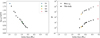 |
Fig. B.1 (Left) Blowout size (sBO,eff) derived from numerical calculations (see Sect. 2.1.3) for main-sequence stars F4-M4 at an age of 4 Gyr (2-3 Gyr for F-type stars). The values for stars later than ~ K2-type are not shown as they do not exist. (Right) Minimum values of ψ are required for sBO,eff to exist (ψmin,sBO) for stars without radiative blowout size, and their ψ values are estimated in this study (Fig. 3). The star shape indicates the value corresponding to AU Mic from Plavchan et al. (2005). |
B.2 Semi-analytical contrast analyses
While detailed distribution maps are essential for accurately modeling resonant structures relevant to interferometric detection, they can be complemented by a fast, generalized framework for estimating resonant ring strengths. To this end, we now turn to semi-analytical approaches, which offer a computationally efficient means of estimating exozodi levels across a broad range of system parameters without requiring full numerical simulations.
The semi-analytical expression of contrast (Eq. 14) expanded from the formulation of Stark & Kuchner (2008), were used to fit the results presented in Sects. 3.1.2 and 3.2.1. Figure B.2 show the same datasets from the pilot study plotted against the modified expression ![Mathematical equation: $a_\text{p}^{1/2} \left[ \beta_\text{PR} \left(1+\psi\right) \right]^{-1} M_\ast^{-1/2}$](/articles/aa/full_html/2026/06/aa56764-25/aa56764-25-eq37.png) from Eq. (15), along with the improved contrast fits. Since this modified x-axis expression increases with decreasing stellar mass, the data generally follow the order F4, G4, K4, to M4. However, the high ψ value for the M-type star significantly shifts their data toward smaller x-values, altering their relative positions in the plot. Cases with different planetary mass other than 1 M⊕ constitute a small portion of the total dataset due to the dominance of the main study data. This contributes to some deviations of the pilot study data from the modified fits, combined with the uncertainties caused by the small number of particles, as previously mentioned. Nonetheless, the data show overall better agreement under the modified expressions, as seen by comparing Figs. 4 and B.2. Similarly, Fig. B.3 shows a better fit to the main study data using the modified parameters, supporting the utility of the semi-analytical function for approximate estimations.
from Eq. (15), along with the improved contrast fits. Since this modified x-axis expression increases with decreasing stellar mass, the data generally follow the order F4, G4, K4, to M4. However, the high ψ value for the M-type star significantly shifts their data toward smaller x-values, altering their relative positions in the plot. Cases with different planetary mass other than 1 M⊕ constitute a small portion of the total dataset due to the dominance of the main study data. This contributes to some deviations of the pilot study data from the modified fits, combined with the uncertainties caused by the small number of particles, as previously mentioned. Nonetheless, the data show overall better agreement under the modified expressions, as seen by comparing Figs. 4 and B.2. Similarly, Fig. B.3 shows a better fit to the main study data using the modified parameters, supporting the utility of the semi-analytical function for approximate estimations.
From the modified contrast function, the semi-analytical value of the optical depth contrast can be derived using Eqs. (12) and (13) from Stark & Kuchner (2008):
 (B.2)
(B.2)
where nBG is the background surface density of dust, proportional to s-α ∙ tmig ∝ s1-α. The function from Eq. (14) with the best-fit parameters (Eq. 16) is used for the contrast C(s). If the minimum dust size is smaller than the effective blowout size (smin < sBO,eff), the blowout size (see Sect. 2.2.2) is used instead. The resulting semi-analytical values of ⟨Cτ⟩ are 1.71, 4.40, 5.81, and 6.55 for F4, G4, K4, and M4, respectively. These values are comparable to, but ∼ 30% smaller than those directly calculated from the optical depth distributions (see Sect. 3.2.2). The discrepancies reflect limitations in the contrast function (Eq. 14) and fitting uncertainties, since the function is not entirely reliable for extreme values of βPR and Mp, as noted by Stark & Kuchner (2008). Nevertheless, the semi-analytical ⟨Cτ⟩ values can be used to approximately estimate τBG ∙ ⟨Cτ⟩ when the background level of dust is given. Thus, the semi-analytical functions remain valuable as a first-order method for estimating resonant ring optical depths in a variety of cases without conducting intensive simulations.
The presence of the resonant structures can also be inferred from the semi-analytical contrast function. Among the eight discrete sizes used in the main study, the minimum size where the resonant ring appears (sc,min) is approximately 10, 3, 1, and 1 μm for F4, G4, K4, and M4, respectively (Sect. 3.2.1). These values are broadly consistent with the more precise estimates of 14.8, 1.78, 0.70, and 0.18 μm obtained from the fitted functions. A resonant ring structure is expected if the smallest size of dust present in the system is below sC,min, since sC,min typically exceeds the corresponding values of sBO,eff (Sect. 2.2.2). Therefore, the fitted functions provide a way to estimate sC,min and assess the presence of resonant structures. When stellar and planetary parameters and the dust size distribution of a system are known, the semi-analytical approach enables a quick assessment of the likelihood and strength of resonant ring structures.
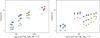 |
Fig. B.2 Same data as Fig. 4, but plotted against the modified term |
![Mathematical equation: $a_\text{p}^{1/2} \left[ \beta_\text{PR} \left(1+\psi\right) \right]^{-1} M_\ast^{-1/2}$](/articles/aa/full_html/2026/06/aa56764-25/aa56764-25-eq39.png)
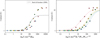 |
Fig. B.3 Same data as Fig. 5, but plotted against the original term |

![Mathematical equation: $a_\text{p}^{1/2} \left[ \beta_\text{PR} \left(1+\psi\right) \right]^{-1} M_\ast^{-1/2}$](/articles/aa/full_html/2026/06/aa56764-25/aa56764-25-eq41.png)
B.3 Alternative results using a different gyrochronology model
While we adopted the conservative value of ψ ∼ 44 for M4-type stars throughout our study, using a higher value of ψ ∼ 127 derived from an alternative gyrochronology model (Lu et al. 2024; see Sects. 3.1.1 and 4.1) causes changes in resonant ring contrast and optical depth trends across spectral types. With this higher ψ, the increase in stellar wind drag can outweigh the effect of decreasing M* (see Sect. 4.3), resulting in an estimated contrast reduction by a factor of ∼ 0.6 for dust size s = 50 μm, as used in the pilot study. This rough estimate is derived from the ratio of contrasts for different ψ values, using the semi-analytical function in Eq. (14). Figure B.4 shows a replotted version of the right panel of Fig. 4, illustrating the expected change when applying this alternative ψ value to M4-type cases in Model II. Under this estimate, the contrasts for M4-type stars become comparable to that of G4-type, and K4-type stars exhibit the highest contrasts. These changes in trend are likewise expected to occur in the contrast values of the main study in Fig. 5.
Similarly, we estimate that the optical depth contrast for M4-type stars would be reduced by a factor of ∼ 0.7 when adopting this larger ψ, based on the semi-analytical function of Eq. (B.2).
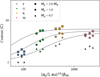 |
Fig. B.4 Right panel of Fig. 4 replotted to show the estimated results when adopting a higher ψ ∼ 127 for M4-type stars, based on the alternative gyrochronology model of Lu et al. (2024). |
This yields an estimated value of ⟨Cτ⟩ ~ 6.92 for M4-type, making it second to K4-type in contrast strength. This comparison is based on the original values of 1.95, 5.98, 8.07, and 9.85 for F4, G4, K4, and M4, respectively (see Sect. 3.2.2). The corresponding maximum optical depths approximated by τBG ∙ ⟨Cτ⟩ would reflect the same change in ordering, with values expected to be around ∼ 6, 18, 24, and 21 zodis for F4, G4, K4, and M4, respectively, after accounting for the different gyrochronology model (see Sect. 4.3). This estimated change also applies to the trend in resonant ring surface brightness, but does not affect the trend in asymmetric flux per beam presented in Fig. 10. In fact, it would reinforce the peak appearing at K-type, since the surface brightness from M4-type systems would further decrease due to their reduced optical depth.
This potentially stronger influence of stellar wind drag in M-type systems would lead to even more rapid dust removal, supporting the stellar-wind-driven explanation for the lack of debris disk detections around old M-type stars, assuming a smooth disk with limited dust production (Sect. 4.2). While our earlier analysis suggested that, in the presence of planet-induced resonant structures, warm exozodis may be more optically thick toward M-type stars than current data indicate (e.g., HOSTS; Ertel et al. 2020; see Sect. 4.3), these alternative estimates imply that resonant trapping produces a slightly larger enhancement of dust around K-type stars. This shift indicates that the predicted optical depth for M-type systems is sensitive to the stellar wind environment and rotational evolution, and may plausibly range from values comparable to G-type stars to levels exceeding those of K-type. Overall, our results suggest that the trend of increasing resonant contrast and optical depth with decreasing stellar mass is generally consistent, though a potential peak or inversion within the K-M spectral range remains.
B.4 Assumptions on stellar evolution and implications for F-type stars
For all simulations and stellar wind drag estimates in this study, we used the same stellar parameters listed in Table 1, assuming that these properties remain largely unchanged over the main-sequence lifetime, as described in Sect. 2.2.1. While this assumption is valid for low-mass stars, it is unphysical for F4-type stars at 4 Gyr, as they have evolved off the main-sequence and would no longer be classified as F4-type. According to MIST stellar evolution models (Choi et al. 2016), the age of 4 Gyr is not applicable to stars with initial masses above ∼ 1.28 M⊙ (earlier than F6), as these stars have evolved off the main sequence by that time. In particular, a star with an initial mass of ∼ 1.38 M⊙ becomes a white dwarf by 4 Gyr.
Since such evolved remnants are observationally rare, and exoplanet detection surveys mostly target main-sequence stars (e.g., Mamajek & Stapelfeldt 2023; Menti et al. 2024), our use of the typical main-sequence parameters remains appropriate. The ψ value for a typical main-sequence F4-type star at nominal ages of 2-3 Gyr would be ∼ 1.21-0.90, which can also be approximately inferred from Fig. 8, slightly higher than the 4 Gyr value under the same stellar parameters. This implies a modest reduction in ring contrast, optical depth, and surface brightness relative to the results of our study if the exact 2-3 Gyr ψ values were used, assuming a constant background level (see Sect. 4.2 and Eq. 14). Consequently, using ψ values more representative of typical main-sequence ages for F-type stars does not alter the overall trend of increasing optical depth toward later spectral types, nor the conclusion that asymmetric exozodi flux per beam is likely brightest around K-type stars.
Therefore, while this approximation introduces some uncertainty, our adopted stellar parameters hold for the scope of this study, and our primary conclusions remain robust.
B.5 Comparison with the mean collisional timescale
We present here the corresponding comparisons from Sect. 4.5 using the mean collisional timescale ⟨tcoll⟩ in place of Eq. (19), to illustrate the sensitivity of our results to the adopted definition.
Adopting the mean collisional timescale ⟨tcoll⟩ shifts the critical size toward smaller grains, implying stronger collisional effects than estimated in Sect. 4.5, particularly for grain sizes beyond the order of a hundred μm. In the absence of planetary perturbations (see Fig. B.5), the comparison between ⟨tcoll⟩ and tmig shows that the steady-state size distribution ∝ s−2.5 still holds for τBG = 3 zodis approximately across the full size range considered in the main study.
When compared with tres (see Fig. B.6), the resonant rings around G, K, and M-type stars would roughly follow the contrasts set by grain sizes of ∼ 30 μm, while F-type stars follow ∼ 300 μm. As implied from Fig. 5, this reduces the estimated values of ⟨Cτ⟩ (to ∼ 5, 4, 2.5 for M, K, G, and ∼3 for F) compared to Sect. 3.2.2, but preserves the overall trend of increasing contrast toward lower-mass stars. Therefore, for the nominal case of τBG = 3 zodis, the main result that K-M-type stars exhibit the strongest resonant ring structures is expected to remain robust regardless of the adopted definition of the collisional timescale. For dustier systems such as τBG = 27 zodis, however, the comparisons based on ⟨tcoll⟩ indicate that our collisionless framework is no longer applicable without explicitly accounting for collisional processes.
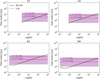 |
Fig. B.5 Comparison of timescales for effective migration driven by PR and stellar wind drags, as in Fig. 11, but using the mean collisional timescale ⟨tcoll⟩. |
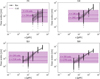 |
Fig. B.6 Comparison of timescales for resonant trapping from simulation data, as in Fig. 12, but using the mean collisional timescale ⟨tcoll⟩. |
Mamajek, E. E., “A Modern Mean Dwarf Stellar Color and Effective Temperature Sequence”, available at https://www.pas.rochester.edu/~emamajek/EEM_dwarf_UBVIJHK_colors_Teff.txt
All Tables
All Figures
|
Fig. 1 (Left) Example of face-on surface density distribution of dust in a planet’s corotating frame, with a K4-type star located at the origin. The white dot indicates an Earth-like planet placed at the inner boundary of the CHZ. A total of 100 dust particles with a size of 50 μm are used. The resonant ring structure is visible around the planet’s position. The color scale indicates surface density in arbitrary units, with lighter colors corresponding to higher densities. (Right) Azimuthally averaged surface density of dust in arbitrary normalized units, based on the distribution in the left panel. The background disk appears as a nearly constant plateau, while the resonant ring structure shows a density enhancement. |
| In the text | |
|
Fig. 2 QPR values for grain sizes s ∼ 0.1300 μm (left) and the corresponding βPR values (right ; analogous to Fig. 7 of Rigley & Wyatt 2020). The solid lines show the numerical values for the different stellar spectral types used in this study, while the dashed lines (right panel) indicate the analytical βPR values using QPR = 1 (Eq. (2)). The black dots mark the discrete grain sizes adopted in the main study. The dotted black line (right panel) denotes βPR = 0.5. Sizes above this threshold, corresponding to grains blown out of the system for circular orbits, are marked with cross (×) symbols. The size ∼50 μm used in the pilot study is safely higher than the blowout size and meets the assumption of QPR ∼ 1. |
| In the text | |
|
Fig. 3 ψ values given by Eqs. (4) and (9) for main-sequence stars of spectral types F4 to M4 at an age of ∼4 Gyr (2-3 Gyr for F-type stars). The four spectral types used in this study are marked in blue, green, yellow, and red, respectively. The dashed line shows ψ = 1, where the stellar wind drag equals the PR drag. |
| In the text | |
|
Fig. 4 Contrast values from the pilot study, plotted against the |
| In the text | |
|
Fig. 5 Contrast values from the main study plotted against grain sizes. Cases where s < sBO,eff are shown as cross (×) marks, which overlap with other data points up to 1 μm. The dashed lines indicate the size-combined contrast values of optical depth |
| In the text | |
|
Fig. 6 Distributions of optical depth (upper row) and surface brightness (10 μm; lower row) for spectral types F4, G4, K4, and M4, from left to right, assuming a constant τBG ∼ 3 zodis. The star is located at the center of the distributions, and the planet is marked with a white dot to the right of the central star. The spatial scale differs between the upper and lower panels: the optical depth maps show a larger region (∼4 ap) to capture the full disk structure, while the surface brightness provides a zoom-in on a smaller region (∼2 ap) around the planet to emphasize resonant ring structures. All panels have a consistent bin size of ap/50 × ap/50. The color bars vary across spectral types to optimize visualization. For reference, the optical depth at r ∼ 2 ap is τBG ≈ 2.1 × 10⁻⁷ for all spectral types. The inner regions of the surface brightness maps are saturated above the ring maximum and excluded within the sublimation distance. The spatial scale also varies with spectral type, with lower-mass stars having more compact configurations. These results correspond to Model II only, as they are from the main study. Note that we derive our results from grain sizes of 0.1-300 μm and may differ if larger grains are included (see Sect. 4.5). |
| In the text | |
|
Fig. 7 Stellar rotation period (P*, left), mass-loss rate (Ṁ*, middle), and ψ (right) for main-sequence stars of spectral types F4-M4 at age 4 Gyr (2-3 Gyr for F-type). Different symbols and colors show results from the three gyrochronology models, with approximate uncertainties. |
| In the text | |
|
Fig. 8 ψ values given by Eqs. (4) and (9) for main-sequence stars of spectral types F4-M4 at an age of 1 Gyr (empty circles), 4 Gyr (2-3 Gyr for F-type stars; filled circles), and 10 Gyr (empty triangles) using gyrochrones from Lu et al. (2024). For 10 Gyr, only values for stars with masses below ∼0.8 M⊙ are shown, as more massive stars have evolved off the main sequence by that age (Choi et al. 2016). The 4 Gyr results are almost identical to those in Fig. 3, except for the larger M4 value due to the change in the gyrochronology model. |
| In the text | |
|
Fig. 9 Asymmetric surface brightness (10 μm; upper row), and corresponding flux per beam relative to the planet flux Fp (lower row), following the format of Fig. 6. The inner regions are saturated above the ring maximum, and all maps are shown within a spatial scale of ∼2 ap. The asymmetric surface brightness maps here follow the approach of Fig. 11 in Defrère et al. (2010). The area within the IWA is masked in the flux per beam maps, assuming d = 10 pc and B = 100 m. For reference, the beam FWHM (λ/B ≈ 0.2 au) is about twice the diameter of the IWA mask. |
| In the text | |
|
Fig. 10 Maximum value of the asymmetric surface brightness of resonant ring at 10 μm (blue, left axis) and the flux per beam (orange, right axis) for each spectral type, assuming a constant background level of ∼3 zodis, grain sizes of 0.1-300 μm, nulling baseline B = 100 m, and distance d = 10 pc. Higher dust levels or the inclusion of larger grains may alter the brightness and fluxes (see Sect. 4.5). Note that the two values are not in scale. |
| In the text | |
|
Fig. 11 Comparison of timescales for effective migration driven by PR and stellar wind drags (solid black lines), evaluated at an age of 4 Gyr (2-3 Gyr for F-type), with the collisional timescale corresponding to the optical depths τBG = 3 and 27 zodis referenced from the HOSTS survey (dashed purple lines; see Sects. 3.2.2 and 4.3). The comparison is made near the position of the planet ∼ap (HZmid). Collisional timescales for a range of face-on optical depths, τ = 1-1000 zodis, are also shown as a purple band (top to bottom). Results are shown for each stellar spectral type as a function of grain size over 0.1-1000 μm, restricted to s ≥ sBO,eff and adapted from Fig. 3 of Najita & Kenyon (2023). |
| In the text | |
|
Fig. 12 Comparison of timescales for resonant trapping from simulation data (black dots) with the median values (solid black lines) and 1σ uncertainties (gray bands), against the collisional timescale corresponding to the maximum resonant ring optical depth of τBG ∙ ⟨Cτ⟩ (dashed purple lines). For each ⟨Cτ⟩ value of ∼2, 6, 8, and 10 for F, G, K, and M-types stars, τBG values of 3 (upper dashed line) and 27 zodis (lower dashed line) are examined (see Sect. 3.2.2). Other plotting conventions are identical to those in Fig. 11. |
| In the text | |
|
Fig. B.1 (Left) Blowout size (sBO,eff) derived from numerical calculations (see Sect. 2.1.3) for main-sequence stars F4-M4 at an age of 4 Gyr (2-3 Gyr for F-type stars). The values for stars later than ~ K2-type are not shown as they do not exist. (Right) Minimum values of ψ are required for sBO,eff to exist (ψmin,sBO) for stars without radiative blowout size, and their ψ values are estimated in this study (Fig. 3). The star shape indicates the value corresponding to AU Mic from Plavchan et al. (2005). |
| In the text | |
|
Fig. B.2 Same data as Fig. 4, but plotted against the modified term |
| In the text | |
|
Fig. B.3 Same data as Fig. 5, but plotted against the original term |
| In the text | |
|
Fig. B.4 Right panel of Fig. 4 replotted to show the estimated results when adopting a higher ψ ∼ 127 for M4-type stars, based on the alternative gyrochronology model of Lu et al. (2024). |
| In the text | |
|
Fig. B.5 Comparison of timescales for effective migration driven by PR and stellar wind drags, as in Fig. 11, but using the mean collisional timescale ⟨tcoll⟩. |
| In the text | |
|
Fig. B.6 Comparison of timescales for resonant trapping from simulation data, as in Fig. 12, but using the mean collisional timescale ⟨tcoll⟩. |
| In the text | |
Current usage metrics show cumulative count of Article Views (full-text article views including HTML views, PDF and ePub downloads, according to the available data) and Abstracts Views on Vision4Press platform.
Data correspond to usage on the plateform after 2015. The current usage metrics is available 48-96 hours after online publication and is updated daily on week days.
Initial download of the metrics may take a while.