| Issue |
A&A
Volume 700, August 2025
|
|
|---|---|---|
| Article Number | A243 | |
| Number of page(s) | 17 | |
| Section | Astrophysical processes | |
| DOI | https://doi.org/10.1051/0004-6361/202450331 | |
| Published online | 25 August 2025 | |
Fast giant flares in discs around supermassive black holes
1
Max-Planck-Institut für Radioastronomie, Auf dem Hügel 69, 53121 Bonn, Germany
2
Institut für Astronomie und Astrophysik, Kepler Center for Astro and Particle Physics, Universität Tübingen, Sand 1, 72076 Tübingen, Germany
3
McWilliams Center for Cosmology & Astrophysics, Department of Physics, Carnegie Mellon University, Pittsburgh, PA 15213, USA
4
Department of Astronomy, University of Illinois at Urbana-Champaign, 1002 W. Green St., IL 61801, USA
⋆ Corresponding author: This email address is being protected from spambots. You need JavaScript enabled to view it.
Received:
11
April
2024
Accepted:
3
June
2025
Abstract
Aims. We studied the thermal stability of non-self-gravitating turbulent α-discs around supermassive black holes (SMBHs) to test a new type of high-amplitude galactic nucleus flares.
Methods. By calculating the disc structures, we computed the critical points of equilibrium curves for discs around SMBHs, which cover a wide range of accretion rates and resemble the shape of a ξ curve.
Results. We find that a transition of a disc ring from a recombined cold state to a hot, fully ionised, advection dominated, geometrically thick state is possible. Such a transition can trigger a giant flare for SMBHs with masses ∼106 − 108 M⊙ if the prior geometrically thin and optically thick disc with convective energy transport surrounded a central radiatively inefficient accretion flow. An increase in the viscosity parameter α is a necessary condition for this scenario. This increase may be related to the fact that the magnetic Prandtl number increases and exceeds 1 during ionisation. When self-gravity effects in the disc are negligible, the duration and power of the flare exhibit a positive correlation with the prior truncation radius of the geometrically thin disc. According to our rough estimates, the mass of about ∼4 − 3000 M⊙ can be involved in the giant flare lasting 1 to 400 years if the flare is triggered somewhere between 60 and 600 gravitational radii from the SMBH of 107 M⊙. The accretion rate on the SMBH peaks about ten times faster at the potentially super-Eddington level. An optically thick outflow with the comparable mass loss rate leads to anisotropy of the emission. At the beginning of the giant flare, the region near the truncation radius is heated to ∼105 K, and its UV/optical luminosity is at least ∼0.3 − 4 LEdd depending on the SMBH mass.
Conclusions. The sudden heating of a cold disc around a SMBH can trigger a massive outburst, similar in appearance to what is proposed to occur after a tidal disruption event.
Key words: accretion / accretion disks / black hole physics / instabilities / galaxies: nuclei / galaxies: active
© The Authors 2025
 Open Access article, published by EDP Sciences, under the terms of the Creative Commons Attribution License (https://creativecommons.org/licenses/by/4.0), which permits unrestricted use, distribution, and reproduction in any medium, provided the original work is properly cited.
This article is published in open access under the Subscribe to Open model.
Open access funding provided by Max Planck Society.
1. Introduction
Disc instability is believed to be one of the underlying causes of transient events in binary systems with accretion discs. For dwarf and X-ray novae, a well-studied scenario of outbursts, the disc instability model (DIM; see e.g. Hameury 2020, and references therein) has been developed, according to which the non-monotonic opacity behaviour related to the partial ionisation of hydrogen drives the thermal-viscous instability. Admittedly, discs in active galactic nuclei (AGN) can also undergo viscous-thermal instabilities (e.g. Mineshige & Shields 1990; Siemiginowska et al. 1996; Menou & Quataert 2001a; Janiuk et al. 2004).
In low-mass X-ray binaries, matter from a normal star may accumulate in a slowly expanding torus around a compact object. As the mass accumulates, the temperature gradually rises and ionisation of the hydrogen eventually becomes possible. Then a notorious opacity dependence on temperature allows a thermal instability (see e.g. Faulkner et al. 1983). The outburst mechanism can be suitably illustrated as a limit cycle on the relationship between the effective temperature Teff or the accretion rate Ṁ and the surface density Σ (called the S-curve; see Fig. 1 or figure 4 in the review by Lasota 2016, also Meyer & Meyer-Hofmeister 1981; Smak 1984b). If the parameters of a particular ring of a disc fall on the negative branch of the S-curve, the ring is unstable. The ionisation instability occurs at temperatures ∼104 K.
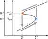 |
Fig. 1. General S-curve at some radius in accretion disc. The limit cycle instability is shown schematically: on the lower branch the mass accumulates, on the upper branch the mass flows out of a ring. |
Another instability is associated with the radiation-pressure-dominated optically thick regime and occurs at higher temperatures. A corresponding limit-cycle behaviour for black-hole discs with accretion rates close to the critical Eddington accretion rate has been previously proposed (Taam & Lin 1984; Lasota & Pelat 1991; Cannizzo 1996; Belloni et al. 1997; Szuszkiewicz & Miller 1998; Janiuk et al. 2000; Janiuk & Czerny 2011; Czerny 2019).
For the present work, we studied the equilibrium curves for discs around SMBHs in a wide range of accretion rates. These equilibrium curves resemble the letter ξ and have two unstable branches, one connected to the partial ionisation instability and the other to the radiation-pressure instability. We find a new scenario of disc heating, triggered by the ionisation instability, which can only occur in a disc around a SMBH and requires that the turbulent α-parameter becomes higher in the ionised state. As the radiation pressure plays a much larger role in discs around SMBH than around stellar-mass black holes (BHs), a situation arises when the two instabilities can occur at the same surface density. This can cause a cold disc ring heated by the ionisation instability to bypass the hot thin state and continue to heat until it becomes geometrically thick, leading to a huge increase in the accretion rate, by a factor of 105 − 106. Such a transition is likely to induce the super-Eddington state, when strong outflows are produced. The high aspect ratio of the optically thick advection-dominated disc explains the relatively short flare duration.
We expect such flares to be observationally similar to tidal disruption events (TDEs), except for the asymmetric manifestations. According to our toy-model estimates, the giant flares can be more powerful and longer than the typical average TDE. The emission from the initial heating is likely to be in the extreme ultraviolet and optical diapason, followed by soft X-rays, which may be strongly attenuated, as is usually expected from the outflowing accretion discs in the unfortunate geometrical situation.
In Sect. 2 we describe an analysis that can be carried out using equilibrium curves, which shows why giant flares are possible. A more detailed description of the conditions for the development of normal and giant flares in discs around SMBH is given in Sect. 3. The basic properties of giant flares are considered in Sect. 4. We further discuss key assumptions for the mechanism and observational implications in Sect. 5, and we summarise in Sect. 6.
In the paper we use the following definition for the Eddington accretion rate:
 (1)
(1)
Here M is the BH mass and the Eddington luminosity is
 (2)
(2)
The Thomson cross-section is denoted by σT and other symbols have their standard meanings.
2. Equilibrium curves and flares
2.1. S-curves
S-curve is a graphically depicted locus of the disc accretion rate Ṁ (or effective temperature Teff) and the surface density Σ at a single disc radius (see Fig. 1). The intervals of an S-curve with a positive slope represent the thermally and viscously stable state of the disc, whereas the negative slope intervals are unstable. To obtain an S-curve one needs to solve the system of equations for the vertical structure of the accretion disc to obtain the relationship between the required values.
In Fig. 2 we depict S-curves in a simplified form to demonstrate how the development of instability leads to an outburst. We neglect for a while a possible change of the turbulent parameter α1. For each radius in a quasi-stationary disc, a proper S-curve can be constructed. The orange and blue points mark the critical surface densities Σ− and Σ+ – the turning points. If the actual Σ of a ring lies within this interval, the ring can exist in either of the two stable states (for a viscous time). We assume that the whole disc is in the stable cold state and gaining material. If the critical density has been accumulated at the radius r1, the ring can ‘move’ from the blue turning point to the upper branch of the S-curve (on a thermal timescale). The ring will heat the neighbouring rings (r2 and r3 in the picture) by the heat diffusion, advection, turbulent diffusion, and work of pressure forces (Menou et al. 1999), and such an avalanche-like process leads to the heating of the disc rings in a significant range of radii. Simplifying the picture, if the heating is triggered at r1 in Fig. 2, the heating wave could reach r3 but no further, since the density there is the minimum possible to allow the ionisation of matter. The velocity of the radial motion of matter in the heated portion of the disc increases and the accretion rate grows, that is, a flare occurs.
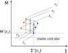 |
Fig. 2. S-curves at different radii r1 < r2 < r3, shown schematically for ionisation instability. When the accretion rate is very low, the whole disc is stable and cold (the bottom line on the plot). If the surface density exceeds the critical value at the innermost radius r1, a heating wave, indicated by arrows, starts outwards, potentially reaching r3. |
In Fig. 3 we plot S-curves for geometrically thin and thick α-discs. The open code ALPHADISC by Tavleev et al. (2023a,b) solves the equations and constructs the S-curves for the geometrically thin α-disc (solid lines, see Appendix A). At higher temperatures, the radiation-dominated regime comprises another negative branch of the Ṁ(Σ) dependence. This regime is also thermally and viscous unstable (Lightman & Eardley 1974; Shakura & Sunyaev 1976; Piran 1978). A hotter positive-slope branch emerges at even higher accretion rates when photon trapping with the radially moving matter (advection) acts as an energy sink at each radius (Abramowicz et al. 1988, 1995; Bjoernsson et al. 1996).
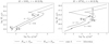 |
Fig. 3. Equilibrium curves for discs around stellar-mass BH (left panel) and SMBH (right panel). In each panel, the ξ-curves are constructed for two values of the turbulent parameter α: 0.1 and 0.01. The solid lines are calculated by ALPHADISC and their upper dotted tails correspond to Prad > Pgas. Analytic relations in the radiation-pressure regime (A zone, dashed, ∝Σ−1) and the advective regime (dash-dotted, ∝Σ) are calculated using Eqs. (B.5) and (B.4), respectively. The dots mark critical points for the geometrically thin states: the minimum and the maximum surface density, Σ+ and ΣA, in the ionised state and the maximum surface density Σ− in the recombined state The arrows schematically show the direction of ring heating due to ionisation instability. At the same time, α increases. |
To construct S-curves for the accretion rates around ṀEdd and higher, one needs to include the non-local energy balance in the equations of the radial structure, while the vertical structure can be taken as vertically integrated (see Sądowski et al. 2011, for a vertical solution). The relativistic super-Eddington disc radial solution was obtained by Sądowski (2009). However, to show the possibility of giant flares, it is not necessary to consider the non-Keplerian character of the flow. The simple analytical relations obtained for the branches of the S-curve of Abramowicz et al. (1988) are sufficient for this purpose.
When the radiation pressure dominates the gas pressure in the geometrically thin disc (called the A zone, Shakura & Sunyaev 1973), the height-integrated viscous stress (or Ṁ) can be expressed algebraically from Σ considering the vertical structure equations (Lightman & Eardley 1974). First, we consider a well-known relation between the accretion rate in a stationary disc and the surface density that follows from the definition of the viscous-stress tensor (Lynden-Bell & Pringle 1974):
 (3)
(3)
Here νt is the kinematic coefficient of viscosity. In the scope of α-ansatz for turbulent viscosity (see Eq. (B.3)) this can be re-written as
 (4)
(4)
Here we have taken into account that the sound velocity ∝z0 ωK, which follows from the vertical hydrostatic balance, where ωK is the Keplerian angular velocity.
For the purposes of the qualitative analysis, we use the well-known facts about the thickness of the disc. In the zone where radiation pressure dominates, the disc thickness is proportional to Ṁ (Shakura & Sunyaev 1973). Accordingly, we get from Eq. (4) that Ṁ ∝ 1/Σ0 and the disc is unstable (see e.g. Lightman & Eardley 1974; Kato et al. 2008). In the advection-dominated zone, z0/r saturates at a constant value (Abramowicz et al. 1988; Lipunova 1999; Sądowski et al. 2011; Lasota et al. 2016; Chashkina et al. 2019), which results in Ṁ ∝ Σ0. These dependencies are essentially shown in Fig. 3 by the dashed and dot-dashed lines, respectively (Eqs. (B.5) and (B.4) are used to plot them, see Appendix B). For the disc aspect ratio in the advective regime we adopt z0/r = 0.5.
2.2. Possibility of giant flares in accretion discs around SMBH
It has been proposed that in the discs around stars and compact stellar remnants, the turbulent parameter α is higher in the ionised material than in recombined material (e.g. Smak 1984a; Meyer & Meyer-Hofmeister 2015). Similarly, we assume different α for a cold recombined disc and a hot fully ionised disc around SMBH, although the decreasing α in the recombined material in AGN discs has been criticised (Menou & Quataert 2001b). Janiuk et al. (2004) studied the magnetic Reynolds number and ambipolar diffusion number and found that they exceed the critical values required for sustained turbulence unless the accretion rate is very low. Nevertheless, α might still depend on the degree of ionisation, as shown for protoplanetary discs by Landry et al. (2013) (see also discussion in Sect. 2.1 of Hameury et al. 2009). Additionally, we show in Sect. 5.1 that, within the partial ionisation regime, the magnetic Prandtl number – which is expected to influence the intensity of saturated turbulence and the value of α – varies strongly and crosses 1, which favours the change of α.
Therefore, assuming that α can change its value, we compare the equilibrium curves for a stellar-mass BH and a SMBH in Fig. 3, constructed as described in Sect. 2.1. In our model, the value αcold is considered viable below the Σ− points, while the value αhot is deemed possible above the Σ+ points of every curve.
The distinction between the S-curves of the stellar-mass BH and the SMBH is strikingly evident. For SMBH disc, the length of the gas-pressure-dominated interval is much shorter; this essentially enables the proposed mechanism, as illustrated for particular parameters. Specifically, for the SMBH disc on the right, the maximum critical surface density Σ− in the cold disc with α = 0.01 is higher than the maximum critical surface density ΣA of the geometrically thin hot ionised disc with α = 0.1.
Thus, if the surface density in the cold state of a SMBH disc exceeds the critical maximum value Σ−, the heating instability can lead to a direct transition of the ring to the advective state, skipping the thin-ionised-disc state. A local stability analysis is insufficient for calculating the course of such a process. However, the central point of the proposed mechanism is the assumption that, if the ring in the diagram (Σ, T) turns out to have such a high surface density that a stable solution only exists at a higher temperature, then the ring should heat up if it does not lose its density faster. This is similar to the classic mechanism in the DIM. The increase in α can occur over thermal time, at least we assume that in the ionised state α is higher.
Some time is required for a transition between the states. In the case of a geometrically thin disc, this time is of the order of the thermal time. In the case of a slim advective disc, whose energy balance is not local (the heating and cooling depends on the radial structure), this time is longer: apparently, it is of the order of the viscous time. Because the slim disc is quite thick, the viscous timescale (r/z0)2 (α ωK)−1 is not much longer than the thermal time (α ωK)−1. Thus, we expect that over a characteristic viscous time, the heated rings of the disc travel upwards in temperature with some change in surface density. Whether this change is a decrease or an increase depends on the radius of the ring. At the same time, the accretion rate on the central BH increases.
The evolution of the accretion rate on the SMBH depends on how the size of the advective zone decreases with time and on the outflows from the disc surface. As with outbursts in the DIM, the duration of the flare can be estimated using the viscous time at the maximum radius rmax of the advective zone:
 (5)
(5)
This time can be an order or two longer than the orbital time 1/ωK because α ∼ 0.1 and Π1 ∼ 4−8 (see Appendix B). This time is much shorter than the viscous evolution time in the geometrically thin disc around the SMBH due to the fact that z0/r ∼ 1 in the advective regime and z0/r ∼ 10−3 for a thin disc. Substituting the characteristic values, one obtains
 (6)
(6)
where
 (7)
(7)
In the following section, we abandon the analytical approximations for the upper branches of the ξ-curves and calculate them numerically. We continue to call them S-curves.
3. Flares in discs around SMBH
3.1. Turning points of equilibrium curves
The critical values of the equilibrium curves affect the possibility of a giant flare and its amplitude. To find these values,
 (8)
(8)
we constructed a set of S-curves (see example in Fig. 4, the upper panel) for different SMBH masses.
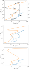 |
Fig. 4. S-curves for 107 M⊙ at r = 100 RS for two values of turbulent parameter αcold = 0.01 (blue) and αhot = 0.1 (orange). The branches ‘A-zone’ and ‘Advection’ were calculated using the code from Lipunova (1999). The accretion rate in absolute units shown on the left axis and in the Eddington rates (1), on the right (upper panel). Temperature Tc in the symmetry plane (middle panel). The dashed line shows the S-curve for αcold without convection. Relative semi-thickness z/r (bottom panel). |
The lower parts of the S-curves, where the gas pressure dominates, are calculated using the open code ALPHADISC (see Appendix A). To calculate upper parts of S-curves, for accretion rates around ṀEdd and higher, advective models (for many Ṁ) must be calculated. An advective disc model requires the calculation of the radial structure, since the local energy balance is violated in a thick disc. Such calculations were performed using the code from Lipunova (1999) (hereafter, L99) for the super-Eddington Keplerian disc. The upper and lower parts of the S-curve are stitched at a point in the hot-disc interval between Σ+ and ΣA, where the disc is geometrically thin. For further details, see Appendix C.
Code L99 can calculate the disc structure with or without a super-Eddington outflow. Although the super-Eddington accretion disc is expected to generate strong winds, the critical values of the turning points are not affected by this. Therefore, to plot the S-curves in the present work we used the option without outflow in L99.
The resulting dependencies of the critical values (8) are shown in Fig. 5 for SMBH mass 107 M⊙. As described above, Σ− and Σ+ are calculated using the ALPHADISC code, ΣA and Σadv are calculated using the L99 code. Only one curve Σ− is calculated with α = αcold, and others, with α = αhot. A giant flare can happen if Σ−(αcold) > ΣA(αhot). Critical Σ− = ΣA ∼ 7 × 10⁴ g cm−2 for 106 − 108 M⊙ SMBH for specific αhot, αcold, and chemical abundance (see Fig. D.3).
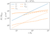 |
Fig. 5. Critical values of surface density (8) for M = 107 M⊙. The viscous parameter is αcold = 0.01 for Σ− (blue line) and αhot = 0.1 in all other dependencies (orange lines). The relations ΣA and ΣA′ show the results of different codes (see Sect. 3.1). |
In Fig. 4, the middle panel, we also show the equilibrium curve for a disc calculated by ALPHADISC without convection by the dashed line. This shows that ignoring convection reduces the critical surface density, as already discussed, for example, by Pojmanski (1986), Cannizzo & Reiff (1992). Our values of Σ− agree well with the results of Hameury et al. (2009), who included convection.
The aspect ratio of the advective disc is greater than 1 in Fig. 4, the bottom panel. This can be attributed to the approximate character of the vertical structure approach in the code L99 (in the original paper Π1 = 1, which decreases the thickness). Here we keep Π1 constant (equal to 6) along the upper S-curve as we are most interested in calculating ΣA. In the following analysis (see Sect. 4) we assume a value of z0/r = 0.5 for the thickness of the advective slim disc.
In general, the ALPHADISC code encounters numerical difficulties when the radiation pressure is significant. However, in certain instances, we have been able to identify the turning points, designated as ΣA′(r). The resulting dependence is plotted in Fig. 5 by the long dashes. It can be seen that at the radii, where the turning points ΣA′ have been successfully identified by ALPHADISC, the value is less than that obtained via the L99 code. For further analysis, we use the ΣA(r) dependence.
3.2. Flares in geometrically thin discs reaching innermost orbit
In this subsection, we shall examine the implications of the found critical densities (Fig. 5), if a disc is geometrically thin down to the innermost orbit. We consider discs around SMBH with mass 107 M⊙.
In Fig. 6, the upper panel, we show the quasi-stationary-disc surface density distributions Σstat(r) computed by ALPHADISC for several values of the accretion rate. In fact, in the real disc, such a density distribution cannot be found to the left of the point where the density exceeds the critical value Σ−(r) and the disc becomes unstable. Accordingly, in the middle and bottom panels we cut the surface density distributions at the intersections with Σ−(r). Similar plots for other SMBH masses can be found in Fig. D.3.
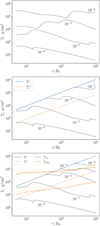 |
Fig. 6. Quasi-stationary surface density Σstat(r) for M = 107 M⊙ and α = αcold at several values of Ṁ, indicated in the graphs in units of ṀEdd (upper panel). Radial distributions of the critical points Σ+ for αhot and Σ− for αcold together with the stationary distributions (middle panel). The latter are shown only for Σstat < Σ−. Superimposed are the radial dependencies of the critical points ΣA and Σadv for αhot (bottom panel). In all panels, αcold = 0.01 (blue) and αhot = 0.1 (orange). The curves are plotted starting from 5RS. |
In the quiescent epoch, as the mass accumulates in the disc due to income of the galactic matter, in its innermost parts the accretion rate Ṁ slowly increases. We imagine that the grey curves change successively in time, replacing each other in order from bottom to top2.
As long as Ṁ ≲ 10−7 ṀEdd, the whole disc is in the stable cold state (this accretion rate roughly corresponds to the intersection of Σ−(r) with a grey curve Σstat(r) at the inner disc edge). Nowhere in the disc do the surface density and temperature reach values where hydrogen ionisation triggers the instability.
When the quasi-stationary accretion rate exceeds ∼ 10−7 ṀEdd, the surface density Σstat becomes greater than Σ− near the inner edge of the disc (see Fig. 6, the middle panel). At this radius Σ− < ΣA (see Fig. 6, the bottom panel). This means that the outburst can occur in the classical framework of the DIM. There will be a transition from the ‘Cold disc’ branch to the ‘Hot disc’ branch near the inner edge of the disc (Σ is between Σ+ and ΣA), and the hot front will start to propagate outwards. A rebrightening of the disc also occurs. The accretion rate on the SMBH increases, resulting in a slow outburst with the characteristic time tvis ∼ 5 ⋅ 104 yr, found from (5) by substituting z0/r ∼ 0.002 (cf. Fig. 4, the bottom panel) and rmax ∼ 60 RS. (Value rmax can be roughly estimated as the intersection of the grey curve for 10−7 ṀEdd and the curve Σ+(r), see Fig. 6, the middle panel).
At the end of the outburst, as the cooling front moves towards the centre and the disc surface density falls below Σ+, the disc moves to the lower cold branch of the equilibrium curves at each radius. The transition to the lower stable branch is actually possible for any Σ in the interval from Σ+ to Σ−. In that respect the left arrow in Fig. 1 is drawn very tentatively. Due to the external influx of matter, the process can start anew. The time between these flares corresponds to a long viscous time in a geometrically thin cold disc with α = αcold.
3.3. Conditions for a giant flare
There are strong indications that to explain the spectral features of some low-accretion-rate accretion discs around BHs (both supermassive and stellar), it is necessary to assume that a geometrically thin disc is truncated from the inside and its inner part is replaced by a high-temperature and low-density accretion flow (see e.g. Yuan & Narayan 2014; Nemmen et al. 2014; López et al. 2024).
The absence of a standard disc at small radii means that, compared to the situation outlined in Sect. 3.2, the quiescent accretion rate should increase to higher values until an instability is triggered. (Because the critical Σ− grows with the radius.) The same considerations underlie the DIM model of Dubus et al. (2001) for the evolution of X-ray transients in binary systems to explain their quiescent times.
For example, the disc around a 107 M⊙ black hole can be truncated at the radius Rtrunc ∼ 40 RS. In this case, the quiescent accretion rate must exceed 10−5 ṀEdd to trigger an outburst similar to the one described in Sect. 3.2, when the ring goes into the geometrically thin hot-disc state (Σ− < ΣA at 40 RS, see Fig. 6, the bottom panel). In particular, if Σ is close enough to ΣA, the increased accretion rate from this ring inwards will be such that the inner part of the disc, at r < 40 RS, will be in the radiation-pressure instability zone (the A zone). The radiation-pressure instability was suggested to drive fluctuations, explaining a particular class of Changing-Look AGN (e.g. Śniegowska et al. 2023).
In contrast, when the truncation radius Rtrunc is even larger, the critical density is so high (Σ− > ΣA at Rtrunc) that a giant flare occurs. For M = 107 M⊙ this happens when Rtrunc ≳ 60 RS. This lower limit for the truncation radius is determined by the intersection of the curves Σ−(r) and ΣA(r) (see the bottom panel in Fig. 6) and depends on the assumed parameters: αhot, αcold, and chemical composition.
The truncation radius Rtrunc itself cannot be determined within our model but it is crucial for the flare properties. It directly determines the accretion rate before a giant flare, which is the critical value of the accretion rate at the turning point (point Σ− in Fig. 4). Figure 7 shows the accretion rate before the flare Ṁbefore versus the truncation radius Rtrunc for different SMBH masses. We plotted the dependencies only for those truncation radii that are larger than the minimum that allows a giant flare to occur. When the truncation radius is smaller than shown in Fig. 7, the thermal instability results in a ‘normal’ outburst and cannot heat the disc to the super-Eddington regime. The maximum value of Rtrunc is determined by the self-gravity limit (see Eq. (10) below).
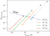 |
Fig. 7. Accretion rate vs truncation radius of thin disc before giant flare. The predicted dependence between the accretion rate and the ADAF outer boundary (9) is also shown. The crosses mark the radius constraint due to self-gravity following (10). The transparent dashed style indicates the Rtrunc region excluded from further analysis. |
We can analyse the truncation radii proposed in the model of an advection-dominated accretion flow (ADAF; Narayan & Yi 1994) replacing the central part of the thin disc (Narayan 1996; Esin et al. 1997; Narayan et al. 1997; Poutanen et al. 1997; Dubus et al. 2001; Menou & Quataert 2001a; Janiuk et al. 2004; Hameury et al. 2007; Narayan & McClintock 2008). To find a transition radius, one needs to consider the physical conditions leading to the formation and thermal structure of the transition region (see e.g. Yuan & Narayan 2014). Czerny et al. (2004) examined the data from the Broad Line Regions using optical/UV spectra from the Large Bright Quasar Survey and found evidence for a ‘strong ADAF principle’: the geometrically thin solution is chosen by the disc only if it is the only solution available for certain Σ. Accordingly, an estimate of the radius of the boundary between the ADAF and the standard disc is as follows:
 (9)
(9)
The inverted relation (9) is shown in Fig. 7. Taking into account condition ṀADAF/ṀEdd ≲ 10−2 (Narayan & Yi 1995), we infer that there is potentially a wide parameter space allowing giant flares to occur. Obviously, the required accretion rates Ṁbefore and Rtrunc depend on the ratio αhot/αcold; they grow as the ratio decreases.
It should be noted that the processes underlying the transition between an ADAF and a cold disc are far from being fully understood. Furthermore, proposals similar to (9) usually presume that α is the value in the ADAF. However, various estimates for the transition radius fall in a rather broad range, qualitatively agreeing with the interval lg(Rtrunc/RS)≈1 − 3 (see refs. in Czerny et al. 2004; Taam et al. 2012; Yuan & Narayan 2014, their figure 7). The values predicted by the purple ‘ADAF’ line in Fig. 7 all give Ṁbefore/ṀEdd ∼ 10−3, and thus can serve as reference values.
4. Energetics and duration of giant flares
Similar to the DIM scenario, the ring heated by the instability can trigger a transition wave (a heating wave) that moves outwards. How far out can such a wave travel? The maximum possible distance Rout,max is determined by the condition that Σstat there (before the flare) should not be less than Σadv (see Fig. 4, the upper panel). This can be difficult to achieve in a ‘rapidly changing landscape’ because, for example, viscous evolution occurs on almost the thermal timescale. We suggest that the minimum extent of the heating wave Rout − Rtrunc is of the order of z0(Rtrunc), assuming isotropic heat diffusion.
At a certain radius in the disc, Rsg, the effects of self-gravity begin to take effect. The distance beyond which the razor-thin disc becomes gravitationally unstable is defined by the following condition (Safronov 1960; Toomre 1964):
 (10)
(10)
The behaviour of the disc and Σ(R) beyond Rsg depend on the cooling and heating mechanisms there. Given the uncertainties in the disc structure, which are beyond the scope of the present work, we chose to present the results only for radii less than Rsg. Also, due to numerical difficulties, we have not calculated flare parameters for Rtrunc very close to Rsg, nor have we considered radii larger than 103 RS, as our primary focus is on lower estimates. The radii Rtrunc that we have included in calculations are indicated by the solid intervals of the curves in Fig. 7.
The time before the flare peaks can be estimated as the heating front propagation time (Meyer 1984):
 (11)
(11)
Alternatively, the time before the peak for a ring viscously spreading from radius Rout in the classical solution of Lynden-Bell & Pringle (1974) is tpeak = tvis/9 (see Appendix D). Both times are of the same order for the slim disc: tpeak ∼ tfront Rout/z0 if Π1 = 6 (see Eq. (B.2)).
The mass of the disc involved in the flare is as follows:
 (12)
(12)
We neglect here the evolution of the surface density that occur as the heating front propagates and that the quiescent Σ(r) could be somewhat higher than Σstat (see footnote 2).
The characteristic flare decay time is the viscous time at the outer boundary of the disc involved in the flare, Rout2/νt(Rout) (see Eq. (5)). Finally, the peak accretion rate can be approximated as the mass divided by the characteristic time (see Eq. (D.4)):
 (13)
(13)
It should be remembered that a substantial fraction of the ‘heated’ mass can be blown away with the outflow, up to (1−ṀEdd/Ṁflare) if one applies the estimate for a super-Eddington disc by (Shakura & Sunyaev 1973).
It is evident that the truncation radius Rtrunc determines Σstat and Ṁbefore before the flare, as well as the power and duration of the flare itself.
Figure 8 shows the calculated parameters of the flares for 107 M⊙: peak accretion rate estimate (13), front time (11) and viscous time (5), accretion rate in a thin disc before the flare, and the mass involved in a flare. The left sections of the curves (shown in black) represent the values calculated for the ‘normal’ sub-Eddington flares (see Sect. 3.2). Figure D.2 summarises the flare characteristics for different masses of SMBH.
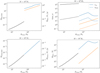 |
Fig. 8. Outburst properties for normal (black) and giant flares (blue and orange) vs. inner truncation radius of quiescent geometrically thin disc. Peak accretion rate (13) (upper left); Characteristic times, calculated using (11) for the flare evolution before the peak and (5) for the characteristic flare duration (upper right); Inner disc accretion rate before the flare (bottom left); Mass involved in a flare (bottom right). The blue curves show the upper limit, obtained if the disc is heated to the radius Rout,max. The orange curves represent the lower limit following assumption Rout = Rtrunc + z0 (see Sect. 4). |
For the giant flares, which are faster and more luminous, we plotted two sequences: assuming Rout = Rout,max≡ min(R (Σstat = Σadv), Rsg), in blue, and Rout = Rtrunc + zo(Rtrunc) = 1.5 Rtrunc, in orange. For ‘normal’ flares, we used Rout = min(R (Σstat = Σ+), Rsg), cf. Fig. 2. The non-monotonic behaviour of the blue curves for Rtrunc ≳ 200RS is explained by the fact that, according to our assumption, the maximum radius that the heating wave can reach is limited by the radius of the gravitational instability Rsg.
Table 1 is a compilation of the flare characteristics for Rout = 1.5 Rtrunc:
 (14)
(14)
Peak accretion rate, characteristic duration, and mass involved in giant flares.
Here the surface density is normalised to 105 g cm−2, α to 0.1, and mass to 107 M⊙. These estimates are the most conservative and do not virtually depend on the radial distribution of the surface density in the quiescent disc.
The maximum effective temperature of the heated ring at radius r can be roughly estimated as the effective temperature at the uppermost branch of the S-curve, assuming that all heat is radiated. For a stationary disc without advection the local viscous flux  , where Ṁ is substituted from Eq. (B.4). Consequently,
  and the maximum Teff ∼ 105 K, provided the heating front does not advance significantly beyond Rtrunc. The luminosity of the heated ring, approximated as σTeff4 r2, is as follows:
 (15)
(15)
This translates into the range ∼0.3 − 4 LEdd for the cases listed in Table 1. The corresponding central accretion rate is super-Eddington (see the 1st line in (14)); the following relation can be constructed: Ṁflare/ṀEdd ∼ 40 (Rtrunc/100 RS LUV/opt/LEdd for Rout = 1.5 Rtrunc.
In the super-Eddington regime, matter is expected to be blown away from the disc, mainly from the radii of order of the spherisation radius (Shakura & Sunyaev 1973). The luminosity LUV/opt would not show a plateau at values (15), because there is no continuous input of matter from the outer radii beyond Rout at a sufficient rate (an optical plateau is possible, however, at a lower luminosity later, see Sect. 5.2). Emission in the harder spectral range, produced by the central part of the disc, can be levelled either because of the outflow regulation mechanism, or because of the photon trapping (advection), or a combination of both. Similarly to the situation of super-Eddington sources in binary systems (Poutanen et al. 2007), an anisotropy of the observed emission from the giant flares is expected during the outflow phase.
It is important to note that while the annuli up to Rout become as hot as required by a slim disc solution, further out the cold disc may experience a less intense heating and reach the stable geometrically thin hot-disc branch (see Fig. 4, the upper panel). This part of the disc becomes optically bright, Teff ∼ 104 K, for characteristic z0/r ∼ 0.005, and evolves quite slowly (see also Sect. 5.2).
5. Discussion
5.1. Critical assumptions of the model
The proposed model is currently based on local S-curve analysis. Numerical simulations show that the trajectories of the parameters of the disc ring during the development of a flare can be quite complicated, even in the case of ‘normal’ flares (see for example, Lasota (2001), figures 11 and 12, Śniegowska et al. (2023), figure 5). In order to confirm the viability of giant flares, it is important to conduct numerical modelling.
Another possible difficulty is a difference between αcold and αhot required by the mechanism. Overall, a change of α fits well within the modern paradigm (e.g. Martin et al. 2019). However, doubts were expressed that α changes between ionised and cold state in AGN discs (Menou & Quataert 2001b) on the grounds that the magnetic Reynolds number does not decrease below the critical value in the cold state, and the MHD turbulence is thus still viable.
We present here the argument in favour of α changing with the temperature in AGN discs. It was suggested by Balbus & Hawley (1998) that the magnetic Prandtl number Prm influences the saturated value of the stress tensor for MHD turbulence and affects the value of α (see also Potter & Balbus 2014, 2017, and references therein). The value Prm ∼ 1 may be a critical value in this regard. At the same time, Potter & Balbus (2014) underlie the dominance of radiative viscosity in the central zones of the accretion discs around stellar-mass objects. Taking into account the radiative viscosity, we have calculated the magnetic Prandtl number for the AGN disc along the S-curves and found that Prm passes through the value 1 in the range of parameters corresponding to the lower unstable branch (related to the hydrogen partial ionisation, see Fig. 9 and Appendix E).
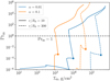 |
Fig. 9. Magnetic Prandtl number calculated for disc around M = 107 M⊙ for α = 0.1 and 0.01 and radii 10 and 300 RS. The dots mark the locations of the critical surface densities Σ−. |
In non-ideal MHD simulations α was found to change by a factor of ∼few×(1 − 10) with the magnetic Prandtl number varying from ∼1 to 102 (Guilet et al. 2022; Held et al. 2024). In this paper, we assume that α varies by a factor of 10. Reducing the value of the assumed α shift would lead to an increase in the minimum truncation radius, which, in turn, would increase the predicted magnitude of a flare.
Observationally, assuming a thermal timescale for the underlying variability mechanism, estimates for αhot in the case of AGN have been obtained with a broad variety of results. By studying the UV/optical spectral variability of 26 AGN Siemiginowska & Czerny (1989) obtained α = 0.001 − 0.1 and for 49 AGN Starling et al. (2004) obtained 0.01 − 0.03, with L/LEdd = 0.01 − 1. Xie et al. (2009) compared observed variability timescales of 31 gamma-ray loud blazars (with L/LEdd = 0.02 − 0.2) with the thermal timescale of α-disc models and got α = 0.1 − 0.3. An analysis by Kelly et al. (2009) of R-band light curves as of a continuous-time stochastic process for 100 quasars provided a lower α ∼ 0.001. Another study of stochastic variability in the optical and UV domain yielded α ∼ 0.05 in 67 AGN (Burke et al. 2021).
5.2. Giant flares and Tidal Disruption Events (TDE)
TDEs can explain bright X-ray, UV and/or optical events in galactic centres lasting months to years (Hills 1975; Rees 1988). If a star passes close enough to a SMBH, and if the tidal forces exerted by the massive object are strong enough, the star can be ripped apart. After returning to the circularisation radius, which is estimated to be twice the tidal radius Rtidal = R⋆ (M/M⋆)1/3,
 (16)
(16)
some debris is thought to form a viscously evolving disc (Cannizzo et al. 1990; Ulmer 1999; Shen & Matzner 2014). A disc of stellar debris, if promptly circularised, heats up and emits in a wide range of wavelengths, from optical to X-ray. Alternatively, radiation is produced directly by stream collisions (Piran et al. 2015; Jiang et al. 2016; Ryu et al. 2020). The sudden increase in brightness is one of the key features used to identify a TDE.
The giant flares involve accretion in the super-Eddington regime, which makes their manifestation similar to that of TDEs (e.g. Shen & Matzner 2014; Komossa 2015; Metzger & Stone 2016; Dai et al. 2018). As TDEs, giant flares from disc instability can be sources of ultra-high-energy cosmic rays (Farrar & Gruzinov 2009).
While the origin of the early emission of TDEs is debated, it is believed that at later times radiation has to originate in the accretion disc. van Velzen et al. (2019) have found that optical light curves of TDE with BH masses < 106.5 M⊙ manifest a flattening at late times that can be explained by an evolving disc (Mummery & Balbus 2020; Mummery et al. 2024). In giant flares, a similar evolution is possible if some disc annuli transfer to the middle stable branch of the S-curve, where the hot Shakura-Sunyaev model applies, and Ṁ ∼ 10−3 − 10−1 ṀEdd (see Fig. 4, the upper panel). The viscous time of the standard hot disc with z0/r < 0.01 is very long,
 (17)
(17)
with Π1 = 6 substituted. On this timescale, the effective temperature of such a remnant disc evolves quite slowly until the disc returns to the cold-disc state.
In general, the viscous time of the advection-dominated flow, as shown in Table 1, is not less than one year, which contrasts with the typical duration of most TDEs. However, care should be taken when comparing observed times and the viscous timescales: the e-folding time of a flare is about 0.4 times shorter than tvis (see Eq. (D.1)), and the rise time is about 0.1 tvis (see Eqs. (11) and (D.3)). It should be noted that longer TDEs sometimes occur (Kankare et al. 2017; Lin et al. 2017; He et al. 2021; Yan & Xie 2018; Zhang 2023; Subrayan et al. 2023; Bandopadhyay et al. 2024; Kumar et al. 2024). At this stage, we do not consider our flare parameters to be restrictive, as they are derived from the simplest estimates of the viscous disc evolution model. The parameters given in Table 1 are physically the upper limits for actual giant flares, taking into account that (i) accretion discs with a shrinking outer boundary evolve faster than those with a fixed outer boundary, (ii) outflows from radii comparable to the outer disc radius accelerate the evolution3.
Estimates of the accretion rates in the TDE disc can be obtained from the spectral fitting of X-rays (Wen et al. 2020, 2021). Using a spectral model for the relativistic slim disc, the SMBH mass and spin can be restricted, as well as the accretion rate entering the hole, which is sometimes super-Eddington. In three cases, it was inferred that a subsolar mass has passed through a disc. A way to estimate the mass rate in a possible super-Eddington outflow from X-ray spectral observations was also suggested (Xiang et al. 2024).
Spectral line shapes of TDEs are used to extract the geometry and kinematics of the photoionised gas. In some works, the interpretation based on the expanding spherical outflow is preferred (Hung et al. 2019; Charalampopoulos et al. 2024). Kara et al. (2018) found evidence for an ionised outflow with a velocity of 0.2c in ASASSN-14li at early times. Using the ionisation parameter ξ = Lx/(n R2)∼103, they obtained the upper limit on the outflow rate Ṁ = 4π mH vout Lx/ξ ∼ 103 M⊙yr−1. Matsumoto & Piran (2021) applied the ‘reprocessing-outflow’ model of the optically thick quasi-spherical wind and, for a sample of observed TDEs, they concluded that the outflows were too massive, about an order of magnitude higher than the mass available in the TDE scenario (1M⊙). The giant flare scenario could help to resolve this issue. The masses involved in giant flares are not less than one solar, typically at least ∼10 M⊙ (see Fig. 10), which shows the dependence between the mass and viscous timescale, obtained within the conservative estimate for the size of the heated zone of the disc, Rout = Rtrunc + zo(Rtrunc).
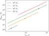 |
Fig. 10. Disc mass (12) involved in giant flare vs viscosity time (5). The dots mark the values corresponding to the ADAF truncation radius (9), shown in Fig. 7. |
The emission from a giant flare is anisotropic due to outflows. However, this fact cannot be used to distinguish them, since anisotropy is an essential part of the ‘unification scheme’ for TDEs as well (Dai et al. 2018; Thomsen et al. 2022; Parkinson et al. 2025).
Sometimes, observations strongly suggest that a TDE event preceded the outburst. For example, spectroscopic observations of AT 2020zso indicate the elliptical geometry of the emitter (Wevers et al. 2022). Further, event AT 2019azh shows signatures of both the stream-stream collision and delayed accretion (Liu et al. 2022). Linearly polarised optical emission at the level of ∼25 per cent observed from AT 2020mot possibly indicate accretion disc formation, when ‘the stream of stellar material collides with itself’ (Liodakis et al. 2023). The alignment of the jet or outflow direction with the perpendicular to the galactic dust plane (Uno et al. 2025) favours the giant flare scenario and argues for the TDE otherwise (Mattila et al. 2018).
Figure 11 depicts the minimum truncation radius necessary for the ionisation instability to trigger a giant flare versus the SMBH mass. The required truncation radius decreases with mass; in particular, for SMBH with M ≳ 109 M⊙, any outburst in a disc with αhot = 0.1 and αcold = 0.01 will be a giant flare, provided that the geometrically thin accretion disc exists at the accretion rates Ṁ lower than 10−5 ṀEdd. We also plotted the circularisation radius Rcirc for stars of different masses, where dependence R⋆(M⋆) for the main sequence stars was used (Kippenhahn et al. 2012). It can be seen that the tidal disruption of a sufficiently massive star can trigger a giant flare by adding material to the cold disc. For example, in the simulations by Andalman et al. (2022), the fallback following the complete destruction of a 1 M⊙ star near a 106 M⊙ SMBH results in a disc up to 200 RS.
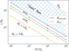 |
Fig. 11. Truncation radii of thin discs and SMBH masses allowing giant flares (hatched area). The upper boundary corresponds to self-gravitation instability radius Rsg. Also shown are the circularisation radii Rcirc for stars of 1, 10, and 20 M⊙. |
5.3. Giant flares rates
The process of supplying mass to the central galactic discs during quiescent periods remains unclear (Lodato 2012; Alexander & Hickox 2012). At distances of ∼0.01 pc in the disc, the self-gravity effects such as spiral waves, fragmentation, and subsequent star formation are possible. The influence of these effects on the mass accumulation in the central cold disc is quite complex, as they can both nourish and hinder the feeding of SMBHs (Nayakshin et al. 2007; Hopkins & Quataert 2010). Other possible ways of feeding the central SMBH have also been proposed, for example, by the very low angular momentum gas (King & Pringle 2006).
Candidates for galaxies capable of producing giant flares include low-luminosity AGN (LLAGN) (Yuan & Narayan 2014) and other quiescent SMBHs (Soria et al. 2006; Volonteri et al. 2011) if a geometrically thin accretion disc manages to form at R ≳ 10 − 102 RS. For very massive SMBHs, giant flares may be impossible due to the absence of a cold disc, because the radius of the gravitational instability Rsg/RS decreases with increasing mass.
For low-mass stellar X-ray binaries, it is common to assume that a binary is transient, that is, it experiences outbursts, if the transfer rate from a neighbouring star through the Lagrangian point is between Ṁ− and Ṁ+. The ratio between these values is only ∼2.5 in Fig. 2. Does this mean that only galaxies with such a rate of mass supply can have giant flares? Obviously not, since galaxies in the process of increasing their central accretion rate from very low levels could also be susceptible to giant flares. Assuming that there is a viscous mass supply from a distant reservoir (e.g. a torus of matter) to the cold disc, the upper limit on the time between giant flares is the Lynden-Bell-Pringle peak time tpeak ≈ 0.1r2/νt (see Appendix D) which gives ∼4 × 10⁵ yr (r/100 RS)3/2 (M/107 M⊙), where we have substituted z0/r = 10−3, αcold = 10−2, and Π1 = 6. We note on the one hand the strong dependence on the reservoir distance from the centre. On the other hand, this time is an upper limit since the critical accretion rate need not be the maximum value attained at the peak, and the time required may be an order of magnitude less. Therefore, we cannot consider the above estimate to be very informative.
The situation becomes further complicated when one considers the multiplicity of potential scenarios for fuelling the central discs. For example, events of tidal stripping of stars (‘partial TDE’, see Chen & Shen 2021) can significantly reduce the time between giant flares.
The frequency of ‘complete’ TDE events is currently estimated to be of the order of one per 104 − 105 yr (van Velzen et al. 2020; Saxton et al. 2021; Sazonov et al. 2021; Masterson et al. 2024). Whether giant flares may contribute to events currently attributed solely to TDEs requires further investigation.
6. Summary
We propose a novel mechanism for outbursts associated with the ionisation-viscous instability in the accretion disc. According to our proposal, a massive, cold, recombined, geometrically thin disc with vertical convective energy transfer can transition to a slim, advection-dominated regime within a few thermal timescales, provided that the critical surface density is accumulated. The mechanism is only viable in discs around SMBHs and if the turbulent parameter α is higher in the ionised state than in the recombined state.
For example, if αhot = 0.1 and αcold = 0.01, and the SMBH mass is ≳109 M⊙, the giant flare can develop if the geometrically thin accretion disc exists at accretion rates Ṁ/ṀEdd less than 10−5. Also, any flare due to the ionisation instability in a geometrically thin convective recombined disc around a SMBH with M ≳ 109 M⊙ will be a giant flare.
For a lighter SMBH, a giant outburst can develop if there is a geometrically thin accretion disc and its inner part is truncated by an optically thin, tenuous flow. An ADAF is a compelling candidate for such a scenario. The region near the truncation radius, when heated after the instability has developed, produces a luminosity of order of LEdd.
Estimated peak accretion rates depend on the size of the disc region transitioning to the ionised state and are > 10 ṀEdd, but may be somewhat reduced by strong outflows. The characteristic outburst duration is estimated by the viscous time of a slim disc, which also depends on the size of the region involved in a flare and can range from several months to several years. After a giant flare, the relic is likely to be a slowly evolving geometrically thin hot disc.
The analysis presented here is not intended to provide precise quantitative estimates. The possibility of giant flare development needs to be further investigated using numerical models that can account for non-equilibrium processes in accretion discs.
If confirmed, giant flares could contribute to a variety of bright extragalactic phenomena, such as TDE.
The change of α is not needed to produce an instability cycle when only one type of two instabilities is involved.
In the DIM, the accretion rate increases with radius in a quiescent disc. Consequently, at the large radii, quiescent Σ(r) could be somewhat higher than depicted Σstat(r) in Fig. 6. However, this fact does not change our estimates because the condition at the trigger radius does not depend on the radial distribution at larger radii.
For 107 M⊙, at 100 RS the slim advective disc cannot exist at ≲ 10ṀEdd (see Fig. 4, the upper panel). This shows that the zone of z/r ∼ 1, which is known as the short-viscous-time zone, is shrinking. In this sense, the solution for an expanding disc from Cannizzo et al. (1990) is not applicable.
Acknowledgments
We thank Arman Tursunov, Loren Held, and Steven Shore for the comments. We are grateful to the referee for many helpful suggestions, and to the language editor for corrections. Support was provided by Schmidt Sciences, LLC. for KM. We acknowledge the usage of computing resources of the M. V. Lomonosov Moscow State University Program of Development and the Sternberg Astronomical Institute where this work has been started. AT was supported by the Deutsche Forschungsgemeinschaft under grant WE1312/56–1.
References
- Abramowicz, M. A., Czerny, B., Lasota, J. P., & Szuszkiewicz, E. 1988, ApJ, 332, 646 [Google Scholar]
- Abramowicz, M. A., Chen, X., Kato, S., Lasota, J.-P., & Regev, O. 1995, ApJ, 438, L37 [NASA ADS] [CrossRef] [Google Scholar]
- Agol, E., & Krolik, J. 1998, ApJ, 507, 304 [Google Scholar]
- Alexander, D. M., & Hickox, R. C. 2012, New A Rev., 56, 93 [NASA ADS] [CrossRef] [Google Scholar]
- Andalman, Z. L., Liska, M. T. P., Tchekhovskoy, A., Coughlin, E. R., & Stone, N. 2022, MNRAS, 510, 1627 [Google Scholar]
- Balbus, S. A., & Hawley, J. F. 1998, Rev. Mod. Phys., 70, 1 [Google Scholar]
- Balbus, S. A., & Henri, P. 2008, ApJ, 674, 408 [NASA ADS] [CrossRef] [Google Scholar]
- Bandopadhyay, A., Fancher, J., Athian, A., et al. 2024, ApJ, 961, L2 [NASA ADS] [CrossRef] [Google Scholar]
- Belloni, T., Méndez, M., King, A. R., van der Klis, M., & van Paradijs, J. 1997, ApJ, 479, L145 [NASA ADS] [CrossRef] [Google Scholar]
- Bjoernsson, G., Abramowicz, M. A., Chen, X., & Lasota, J.-P. 1996, ApJ, 467, 99 [Google Scholar]
- Blaes, O. 2014, Space Sci. Rev., 183, 21 [NASA ADS] [CrossRef] [Google Scholar]
- Burke, C. J., Shen, Y., Blaes, O., et al. 2021, Science, 373, 789 [NASA ADS] [CrossRef] [Google Scholar]
- Cannizzo, J. K. 1996, ApJ, 466, L31 [NASA ADS] [CrossRef] [Google Scholar]
- Cannizzo, J. K., & Reiff, C. M. 1992, ApJ, 385, 87 [Google Scholar]
- Cannizzo, J. K., Lee, H. M., & Goodman, J. 1990, ApJ, 351, 38 [NASA ADS] [CrossRef] [Google Scholar]
- Charalampopoulos, P., Kotak, R., Wevers, T., et al. 2024, A&A, 689, A350 [NASA ADS] [CrossRef] [EDP Sciences] [Google Scholar]
- Chashkina, A., Lipunova, G., Abolmasov, P., & Poutanen, J. 2019, A&A, 626, A18 [NASA ADS] [CrossRef] [EDP Sciences] [Google Scholar]
- Chen, J.-H., & Shen, R.-F. 2021, ApJ, 914, 69 [NASA ADS] [CrossRef] [Google Scholar]
- Clouët, J.-F., & Soulard, O. 2021, ApJ, 919, 78 [Google Scholar]
- Czerny, B. 2019, Universe, 5, 131 [NASA ADS] [CrossRef] [Google Scholar]
- Czerny, B., Rózańska, A., & Kuraszkiewicz, J. 2004, A&A, 428, 39 [NASA ADS] [CrossRef] [EDP Sciences] [Google Scholar]
- Dai, L., McKinney, J. C., Roth, N., Ramirez-Ruiz, E., & Miller, M. C. 2018, ApJ, 859, L20 [Google Scholar]
- Dubus, G., Hameury, J. M., & Lasota, J. P. 2001, A&A, 373, 251 [NASA ADS] [CrossRef] [EDP Sciences] [Google Scholar]
- Esin, A. A., McClintock, J. E., & Narayan, R. 1997, ApJ, 489, 865 [NASA ADS] [CrossRef] [Google Scholar]
- Farrar, G. R., & Gruzinov, A. 2009, ApJ, 693, 329 [NASA ADS] [CrossRef] [Google Scholar]
- Faulkner, J., Lin, D. N. C., & Papaloizou, J. 1983, MNRAS, 205, 359 [Google Scholar]
- Guilet, J., Reboul-Salze, A., Raynaud, R., Bugli, M., & Gallet, B. 2022, MNRAS, 516, 4346 [NASA ADS] [CrossRef] [Google Scholar]
- Hameury, J. M. 2020, Adv. Space Res., 66, 1004 [Google Scholar]
- Hameury, J.-M., Menou, K., Dubus, G., et al. 1998, MNRAS, 298, 1048 [Google Scholar]
- Hameury, J. M., Lasota, J. P., & Viallet, M. 2007, in Black Holes from Stars to Galaxies - Across the Range of Masses, eds. V. Karas, & G. Matt, 238, 297 [Google Scholar]
- Hameury, J. M., Viallet, M., & Lasota, J. P. 2009, A&A, 496, 413 [NASA ADS] [CrossRef] [EDP Sciences] [Google Scholar]
- He, J. S., Dou, L. M., Ai, Y. L., et al. 2021, A&A, 652, A15 [NASA ADS] [CrossRef] [EDP Sciences] [Google Scholar]
- Held, L. E., Mamatsashvili, G., & Pessah, M. E. 2024, MNRAS, 530, 2232 [NASA ADS] [CrossRef] [Google Scholar]
- Hills, J. G. 1975, Nature, 254, 295 [Google Scholar]
- Hopkins, P. F., & Quataert, E. 2010, MNRAS, 407, 1529 [Google Scholar]
- Huba, J. 2013, NRL Plasma Formulary (Naval Research Laboratory) [Google Scholar]
- Hung, T., Cenko, S. B., Roth, N., et al. 2019, ApJ, 879, 119 [NASA ADS] [CrossRef] [Google Scholar]
- Janiuk, A., & Czerny, B. 2011, MNRAS, 414, 2186 [NASA ADS] [CrossRef] [Google Scholar]
- Janiuk, A., Czerny, B., & Siemiginowska, A. 2000, ApJ, 542, L33 [NASA ADS] [CrossRef] [Google Scholar]
- Janiuk, A., Czerny, B., Siemiginowska, A., & Szczerba, R. 2004, ApJ, 602, 595 [NASA ADS] [CrossRef] [Google Scholar]
- Jiang, Y.-F., Stone, J. M., & Davis, S. W. 2013, ApJ, 767, 148 [Google Scholar]
- Jiang, Y.-F., Guillochon, J., & Loeb, A. 2016, ApJ, 830, 125 [NASA ADS] [CrossRef] [Google Scholar]
- Kankare, E., Kotak, R., Mattila, S., et al. 2017, Nat. Astron., 1, 865 [NASA ADS] [CrossRef] [Google Scholar]
- Kara, E., Dai, L., Reynolds, C. S., & Kallman, T. 2018, MNRAS, 474, 3593 [Google Scholar]
- Kato, S., Fukue, J., & Mineshige, S. 2008, Black-Hole Accretion Disks - Towards a New Paradigm - (Kyoto, Japan: Kyoto University Press) [Google Scholar]
- Kelly, B. C., Bechtold, J., & Siemiginowska, A. 2009, ApJ, 698, 895 [Google Scholar]
- Ketsaris, N. A., & Shakura, N. I. 1998, Astron. Astrophys. Trans., 15, 193 [NASA ADS] [CrossRef] [Google Scholar]
- King, A. R., & Pringle, J. E. 2006, MNRAS, 373, L90 [NASA ADS] [CrossRef] [Google Scholar]
- Kippenhahn, R., Weigert, A., & Weiss, A. 2012, Stellar Structure and Evolution (Berlin, Heidelberg: Springer, Berlin Heidelberg) [Google Scholar]
- Komossa, S. 2015, J. High Energy Astrophys., 7, 148 [Google Scholar]
- Kumar, H., Berger, E., Hiramatsu, D., et al. 2024, ApJ, 974, L36 [Google Scholar]
- Landry, R., Dodson-Robinson, S. E., Turner, N. J., & Abram, G. 2013, ApJ, 771, 80 [Google Scholar]
- Lasota, J.-P. 2001, New A Rev., 45, 449 [NASA ADS] [CrossRef] [Google Scholar]
- Lasota, J. P. 2016, in Astrophysics of Black Holes: From Fundamental Aspects to Latest Developments, ed. C. Bambi, Astrophys. Space Sci. Lib., 440, 1 [Google Scholar]
- Lasota, J. P., & Pelat, D. 1991, A&A, 249, 574 [NASA ADS] [Google Scholar]
- Lasota, J. P., Vieira, R. S. S., Sadowski, A., Narayan, R., & Abramowicz, M. A. 2016, A&A, 587, A13 [NASA ADS] [CrossRef] [EDP Sciences] [Google Scholar]
- Lightman, A. P., & Eardley, D. M. 1974, ApJ, 187, L1 [Google Scholar]
- Lin, D., Guillochon, J., Komossa, S., et al. 2017, Nat. Astron., 1, 0033 [Google Scholar]
- Liodakis, I., Koljonen, K. I. I., Blinov, D., et al. 2023, Science, 380, 656 [Google Scholar]
- Lipunova, G. V. 1999, Astron. Lett., 25, 508 [NASA ADS] [Google Scholar]
- Lipunova, G. V. 2015, ApJ, 804, 87 [NASA ADS] [CrossRef] [Google Scholar]
- Liu, X.-L., Dou, L.-M., Chen, J.-H., & Shen, R.-F. 2022, ApJ, 925, 67 [NASA ADS] [CrossRef] [Google Scholar]
- Lodato, G. 2012, Adv. Astron., 2012, 846875 [Google Scholar]
- López, I. E., Yang, G., Mountrichas, G., et al. 2024, A&A, 692, A209 [NASA ADS] [CrossRef] [EDP Sciences] [Google Scholar]
- Lynden-Bell, D., & Pringle, J. E. 1974, MNRAS, 168, 603 [Google Scholar]
- Martin, R. G., Nixon, C. J., Pringle, J. E., & Livio, M. 2019, New A, 70, 7 [Google Scholar]
- Masterson, M., De, K., Panagiotou, C., et al. 2024, ApJ, 961, 211 [NASA ADS] [CrossRef] [Google Scholar]
- Matsumoto, T., & Piran, T. 2021, MNRAS, 502, 3385 [Google Scholar]
- Mattila, S., Pérez-Torres, M., Efstathiou, A., et al. 2018, Science, 361, 482 [Google Scholar]
- Menou, K., & Quataert, E. 2001a, ApJ, 562, L137 [Google Scholar]
- Menou, K., & Quataert, E. 2001b, ApJ, 552, 204 [NASA ADS] [CrossRef] [Google Scholar]
- Menou, K., Hameury, J.-M., & Stehle, R. 1999, MNRAS, 305, 79 [Google Scholar]
- Metzger, B. D., & Stone, N. C. 2016, MNRAS, 461, 948 [NASA ADS] [CrossRef] [Google Scholar]
- Meyer, F. 1984, A&A, 131, 303 [NASA ADS] [Google Scholar]
- Meyer, F., & Meyer-Hofmeister, E. 1981, A&A, 104, L10 [NASA ADS] [Google Scholar]
- Meyer, F., & Meyer-Hofmeister, E. 2015, PASJ, 67, 52 [Google Scholar]
- Mihalas, D., & Mihalas, B. W. 1984, in Foundations of radiation hydrodynamics, eds. D. Mihalas, & B. W. Mihalas [Google Scholar]
- Mineshige, S., & Shields, G. A. 1990, ApJ, 351, 47 [Google Scholar]
- Mummery, A., & Balbus, S. A. 2020, MNRAS, 492, 5655 [NASA ADS] [CrossRef] [Google Scholar]
- Mummery, A., van Velzen, S., Nathan, E., et al. 2024, MNRAS, 527, 2452 [Google Scholar]
- Narayan, R. 1996, ApJ, 462, 136 [Google Scholar]
- Narayan, R., & McClintock, J. E. 2008, New Astron. Rev., 51, 733 [CrossRef] [Google Scholar]
- Narayan, R., & Yi, I. 1994, ApJ, 428, L13 [Google Scholar]
- Narayan, R., & Yi, I. 1995, ApJ, 452, 710 [NASA ADS] [CrossRef] [Google Scholar]
- Narayan, R., Barret, D., & McClintock, J. E. 1997, ApJ, 482, 448 [Google Scholar]
- Nayakshin, S., Cuadra, J., & Springel, V. 2007, MNRAS, 379, 21 [Google Scholar]
- Nemmen, R. S., Storchi-Bergmann, T., & Eracleous, M. 2014, MNRAS, 438, 2804 [Google Scholar]
- Paczyński, B. 1969, Acta Astron., 19, 1 [NASA ADS] [Google Scholar]
- Paczynski, B., & Jaroszynski, M. 1978, Acta Astron., 28, 111 [NASA ADS] [Google Scholar]
- Parkinson, E. J., Knigge, C., Dai, L., et al. 2025, MNRAS, 540, 3069 [Google Scholar]
- Paxton, B., Bildsten, L., Dotter, A., et al. 2011, ApJS, 192, 3 [Google Scholar]
- Piran, T. 1978, ApJ, 221, 652 [Google Scholar]
- Piran, T., Svirski, G., Krolik, J., Cheng, R. M., & Shiokawa, H. 2015, ApJ, 806, 164 [Google Scholar]
- Pojmanski, G. 1986, Acta Astron., 36, 69 [Google Scholar]
- Potter, W. J., & Balbus, S. A. 2014, MNRAS, 441, 681 [NASA ADS] [CrossRef] [Google Scholar]
- Potter, W. J., & Balbus, S. A. 2017, MNRAS, 472, 3021 [Google Scholar]
- Poutanen, J., Krolik, J. H., & Ryde, F. 1997, MNRAS, 292, L21 [NASA ADS] [Google Scholar]
- Poutanen, J., Lipunova, G., Fabrika, S., Butkevich, A. G., & Abolmasov, P. 2007, MNRAS, 377, 1187 [NASA ADS] [CrossRef] [Google Scholar]
- Rees, M. J. 1988, Nature, 333, 523 [Google Scholar]
- Ryu, T., Krolik, J., & Piran, T. 2020, ApJ, 904, 73 [NASA ADS] [CrossRef] [Google Scholar]
- Sądowski, A. 2009, ApJS, 183, 171 [CrossRef] [Google Scholar]
- Sądowski, A., Abramowicz, M., Bursa, M., et al. 2011, A&A, 527, A17 [NASA ADS] [CrossRef] [EDP Sciences] [Google Scholar]
- Safronov, V. S. 1960, Annales d’Astrophysique, 23, 979 [NASA ADS] [Google Scholar]
- Saxton, R., Komossa, S., Auchettl, K., & Jonker, P. G. 2021, Space Sci. Rev., 217, 18 [NASA ADS] [CrossRef] [Google Scholar]
- Sazonov, S., Gilfanov, M., Medvedev, P., et al. 2021, MNRAS, 508, 3820 [NASA ADS] [CrossRef] [Google Scholar]
- Schwarzschild, M. 1958, Structure and Evolution of the Stars (Princeton University Press) [Google Scholar]
- Shakura, N. I., & Sunyaev, R. A. 1973, A&A, 24, 337 [NASA ADS] [Google Scholar]
- Shakura, N. I., & Sunyaev, R. A. 1976, MNRAS, 175, 613 [NASA ADS] [CrossRef] [Google Scholar]
- Shakura, N. I., Lipunova, G. V., Malanchev, K. L., et al. 2018, Accretion Flows in Astrophysics (New York: New York) [Google Scholar]
- Shen, R.-F., & Matzner, C. D. 2014, ApJ, 784, 87 [NASA ADS] [CrossRef] [Google Scholar]
- Siemiginowska, A., & Czerny, B. 1989, MNRAS, 239, 289 [NASA ADS] [CrossRef] [Google Scholar]
- Siemiginowska, A., Czerny, B., & Kostyunin, V. 1996, ApJ, 458, 491 [Google Scholar]
- Smak, J. 1984a, Acta Astron., 34, 161 [NASA ADS] [Google Scholar]
- Smak, J. 1984b, PASP, 96, 5 [NASA ADS] [CrossRef] [Google Scholar]
- Śniegowska, M., Grzȩdzielski, M., Czerny, B., & Janiuk, A. 2023, A&A, 672, A19 [NASA ADS] [CrossRef] [EDP Sciences] [Google Scholar]
- Soria, R., Graham, A. W., Fabbiano, G., et al. 2006, ApJ, 640, 143 [Google Scholar]
- Spitzer, L. 1962, Physics of Fully Ionized Gases (New York: Interscience) [Google Scholar]
- Starling, R. L. C., Siemiginowska, A., Uttley, P., & Soria, R. 2004, MNRAS, 347, 67 [NASA ADS] [CrossRef] [Google Scholar]
- Subrayan, B. M., Milisavljevic, D., Chornock, R., et al. 2023, ApJ, 948, L19 [NASA ADS] [CrossRef] [Google Scholar]
- Suleimanov, V. F., Lipunova, G. V., & Shakura, N. I. 2007, Astron. Rep., 51, 549 [Google Scholar]
- Szuszkiewicz, E., & Miller, J. C. 1998, MNRAS, 298, 888 [Google Scholar]
- Taam, R. E., & Lin, D. N. C. 1984, ApJ, 287, 761 [Google Scholar]
- Taam, R. E., Liu, B. F., Yuan, W., & Qiao, E. 2012, ApJ, 759, 65 [NASA ADS] [CrossRef] [Google Scholar]
- Tavleev, A. S., Lipunova, G. V., & Malanchev, K. L. 2023a, MNRAS, 524, 3647 [Google Scholar]
- Tavleev, A. S., Lipunova, G. V., & Malanchev, K. L. 2023b, DiscVerSt: Vertical structure calculator for accretion discs around neutron stars and black holes, Astrophysics Source Code Library [record ascl:2307.011] [Google Scholar]
- Thomsen, L. L., Kwan, T. M., Dai, L., et al. 2022, ApJ, 937, L28 [NASA ADS] [CrossRef] [Google Scholar]
- Toomre, A. 1964, ApJ, 139, 1217 [Google Scholar]
- Ulmer, A. 1999, ApJ, 514, 180 [Google Scholar]
- Uno, K., Maeda, K., Nagao, T., et al. 2025, arXiv e-prints [arXiv:2503.19024] [Google Scholar]
- van Velzen, S., Stone, N. C., Metzger, B. D., et al. 2019, ApJ, 878, 82 [NASA ADS] [CrossRef] [Google Scholar]
- van Velzen, S., Holoien, T. W. S., Onori, F., Hung, T., & Arcavi, I. 2020, Space Sci. Rev., 216, 124 [CrossRef] [Google Scholar]
- Volonteri, M., Dotti, M., Campbell, D., & Mateo, M. 2011, ApJ, 730, 145 [Google Scholar]
- Vranjes, J. 2014, MNRAS, 445, 1614 [Google Scholar]
- Vranjes, J., & Krstic, P. S. 2013, A&A, 554, A22 [NASA ADS] [CrossRef] [EDP Sciences] [Google Scholar]
- Wen, S., Jonker, P. G., Stone, N. C., Zabludoff, A. I., & Psaltis, D. 2020, ApJ, 897, 80 [NASA ADS] [CrossRef] [Google Scholar]
- Wen, S., Jonker, P. G., Stone, N. C., & Zabludoff, A. I. 2021, ApJ, 918, 46 [NASA ADS] [CrossRef] [Google Scholar]
- Wevers, T., Nicholl, M., Guolo, M., et al. 2022, A&A, 666, A6 [NASA ADS] [CrossRef] [EDP Sciences] [Google Scholar]
- Xiang, X., Miller, J. M., Zoghbi, A., et al. 2024, ApJ, 972, 106 [Google Scholar]
- Xie, Z. H., Ma, L., Zhang, X., et al. 2009, ApJ, 707, 866 [NASA ADS] [CrossRef] [Google Scholar]
- Yan, Z., & Xie, F.-G. 2018, MNRAS, 475, 1190 [NASA ADS] [CrossRef] [Google Scholar]
- Yuan, F., & Narayan, R. 2014, ARA&A, 52, 529 [NASA ADS] [CrossRef] [Google Scholar]
- Zhang, X. 2023, ApJ, 948, 68 [Google Scholar]
- Zhdanov, V. 2002, Transport Processes in Multicomponent Plasma (CRC Press) [Google Scholar]
Appendix A: Geometrically thin disc vertical structure
The vertical structure of the accretion disc is described by the system of four ordinary differential equations (see e.g. Shakura et al. 2018), which follows from the mass, energy, and momentum conservation laws:
 (A.1)
(A.1)
 (A.2)
(A.2)
 (A.3)
(A.3)
![Mathematical equation: $$ \begin{aligned} &\frac{\mathrm{d}\Sigma }{\mathrm{d}z} = -2\rho , \\&z \in [0, z_0]. \nonumber \end{aligned} $$](/articles/aa/full_html/2025/08/aa50331-24/aa50331-24-eq23.gif) (A.4)
(A.4)
Here P = arad T4/3 + Pgas is the total pressure, Q is the heating flux, which for an un-irradiated disc equals the viscous flux Qvis, and T is the temperature. The mass coordinate Σ(z) equals to zero at z = z0 and the surface density of the disc Σ0 at z = 0. The last part of (A.2) includes the α-prescription (Shakura & Sunyaev 1973), where the absolute value of the rφ-component of the viscous tensor wrφ = αP, and α is the turbulent parameter (0 < α < 1).
If the energy is transported solely by radiation diffusion, equation (A.3) implies that
 (A.5)
(A.5)
where 𝜘R is the Rosseland opacity coefficient, arad = 4σSB/c is the radiation constant, c is the speed of light. Otherwise, if ∇rad ≥ ∇ad, the convective motions start to transfer energy according to the Schwarzschild (1958) criterion. The corresponding temperature gradient ∇conv is calculated according to the mixing length theory (Paczyński 1969; Kippenhahn et al. 2012; Hameury et al. 1998).
Flux radiated from one surface equals half the viscous heat flux at the same radius when the local energy balance holds:
 (A.6)
(A.6)
For a disc around a BH, the viscous torque  ,
,  is the specific angular momentum, and rin is the inner radius of the disc.
The open code ALPHADISC was developed by Tavleev et al. (2023a,b) to solve the system (A.1–A.4). The main input parameters of the code are: the mass of the central object M, radius r, viscous torque F (or effective temperature Teff, or the accretion rate Ṁ), and turbulence parameter α. The output is P(z), T(z), Q(z), ρ(z), z0, Σ0, and other parameters. The vertical structure equations are complemented by an equation of state (EoS) and an opacity law, for which their tabulated values from the MESA code4 can be used.
By calculating vertical structures for a set of accretion rates Ṁ, the code provides a set of corresponding surface densities Σ0, that is, the S-curves are obtained. The solar chemical composition is assumed throughout this paper.
Appendix B: Self-similarity of the vertical structure
The vertical structure of the disc is almost self-similar when the disc is hot and ionised. One can introduce dimensionless Π-parameters:
 (B.1)
(B.1)
Here Pc, Tc, ρc, and 𝜘c are the total pressure, temperature, bulk density, and opacity in the symmetry plane. Given the values of Π (calculated by ALPHADISC, for example), and knowing ωK, α, Q0 = σSB Teff4 (or Ṁ), one can easily calculate z0, ρc, Σ0, and Tc as functions of radius. The pressure Pc is obtained from an equation of state, for example that of an ideal gas. If the vertical structure equations are not solved, all parameters of Π can be set to 1; this will be the equivalent of averaging equations (A.1–A.4).
The self-similarity of the vertical structure is reflected in the fact that the Π values found after solving system (A.1)-(A.4) vary insignificantly in the stable hot-disc region (Ketsaris & Shakura 1998; Suleimanov et al. 2007; Tavleev et al. 2023a). If the vertical structure is approximated by a polytropic solution with the polytropic index n = 1..3, corresponding Π1 = 2 (n + 1), Π2 ∼ 0.5, Π3 ≈ 1.1, and Π4 ≈ 0.4.
Using Π1, which can be viewed as (ωK z0/vs)2, where the sound velocity vs = (P/ρ)1/2, one can write the viscous time of a disc as
 (B.2)
(B.2)
where νt if determined from the relation between the kinematic coefficient of turbulent viscosity νt and α is obtained from the stress-tensor for Keplerian α-discs:
 (B.3)
(B.3)
We can infer the dependences between Ṁ and Σ0 for Fig. 3 using the definitions of Π. Combining the first and third equation of (B.1)), we obtain
 (B.4)
(B.4)
For zone A, where P = Prad = aradT4/3 and opacity is determined by the Thomson scattering, with Q0 = Qvis at r ≫ rin in (A.6), we obtain
 (B.5)
(B.5)
Appendix C: Slim disc structure
In the solution for the radial structure of a slim disc, the integration scheme of Lipunova (1999) and equations for Π1, Π2, and Π4 are utilised (see Eq. (B.1)) with fixed values of Π. The local energy balance equation is substituted by
 (C.1)
(C.1)
where Q0 and Qvis are the radiation and viscous flux, per one side of the disc (see Appendix A). The disc is assumed to be Keplerian. The advected flux can be expressed as (Chashkina et al. 2019)
 (C.2)
(C.2)
where the dimensionless entropy per particle is
![Mathematical equation: $$ \begin{aligned} s = \frac{5}{2} + \ln \left[ \frac{\tilde{m}}{\rho }\, \left(\frac{2\, \pi \,\tilde{m}\,k\, T}{h^2}\right)^{3/2}\right] + \left( \frac{32 \pi ^5}{45\, c^3\, h^3}\right) \frac{\tilde{m} \,(kT)^3}{\rho } \end{aligned} $$](/articles/aa/full_html/2025/08/aa50331-24/aa50331-24-eq35.gif) (C.3)
(C.3)
and  is the mean mass per particle. The radial velocity is assumed to be z-independent: vr = Ṁ/(2π rΣ0). Taking into account that
  , after some transformations, we obtain
 (C.4)
(C.4)
where β = Pgas, c/Pc and
 (C.5)
(C.5)
The last dimensionless parameter appears because we assume here a fixed vertical effective polytropic index n, defined through the equation for density ρ = ρc (1 − (z/z0)2)n and pressure P = Pc (1 − (z/z0)2)n + 1 (Paczynski & Jaroszynski 1978).
The semi-thickness z0 is found at each radius by a minimisation procedure. Without an outflow, a solution is found by a single integration starting from an external geometrically thin disc, where we set Qadv = 0. The higher Ṁ, the larger the starting radius of the calculation.
The matching of the S-curves involves the following steps: (1) for specific radius r, calculate the S-curve in the geometrically thin regime in the ALPHADISC code to determine dependences of all disc parameters, including Π-values, on Σ0 (see Appendices A and B); (2) identify Ṁ× where Prad/Pgas = 0.5 at r to obtain Π values in the regime when the disc is still thin but quite hot at the same time; (3) for these fixed Π values, calculate radial models (Σ0(r), etc.) of advective discs for different accretion rates Ṁ ≥ Ṁ×; (4) interpolate the results to derive the dependence Ṁ (Σ0) at r. Thanks to the choice of Π and the fact that Πs vary very slowly in the ionised disc, the sequence of equilibrium points for the slim disc (i.e. its S-curve) smoothly matches that for the geometrically thin disc.
Appendix D: Analytic relations for e-folding time and peak accretion rate
If the mass, radius, and viscosity of a spreading ring are known, the time-dependent accretion rate can be found either analytically or numerically. It also depends on the radial boundary conditions in the disc, as illustrated by Fig. D.1, which compares two analytic solutions with different outer boundary conditions.
To estimate the upper limit of the observable time texp, we assume that the hot advective disc during a giant flare can be treated as a Keplerian disc with a fixed outer radius and constant aspect ratio, so that both the viscosity νt(R) and the viscous time tvis = R2/νt are defined by (5). For example, tvis ≈ 1 yr if Rout = 90 RS and M = 107 M⊙. The e-folding decay time of such a disc is related to the viscous time as
 (D.1)
(D.1)
where l is the parameter defined by the viscosity type, introduced by Lynden-Bell & Pringle (1974); l = 1/3 is appropriate for discs with constant aspect ratio. The parameter k1 = 1.24 (Lipunova 2015), and the dimensionless factor in (D.1) is about 0.38.
The peak accretion rate in the solution of Lynden-Bell & Pringle (1974) for the infinite disc is
 (D.2)
(D.2)
with
 (D.3)
(D.3)
(see Appendix of Lipunova 2015).
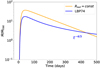 |
Fig. D.1. Analytic solutions for accretion rate evolution in disc without outflow with fixed z0/r (l = 1/3). At late times, the evolution is exponential in the disc with the constant outer radius (orange; Lipunova 2015) and power law, when the outer radius is expanding (blue; Lynden-Bell & Pringle 1974) For the both solutions, the mass is Mflare = 4M⊙ and initial ring radius Rout = 90 RS, which roughly correspond to the minimum flare in a disc around 107 M⊙ SMBH in Table 1. |
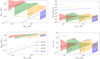 |
Fig. D.2. Outburst parameters for giant flares (coloured areas) and normal flares (dotted lines) vs inner truncation radius of quiescent geometrically thin disc. From top to bottom, from left to right: Mass involved in a flare (14), estimated peak accretion rate (13), characteristic flare duration (5), and rise time (11). The upper boundaries of the coloured areas correspond to the case when the disc is heated to the radius Rout,max, the lower boundaries to the conservative assumption Rout = Rtrunc + z0 (see Sect. 4). The lower grey line illustrates the limits for intermediate masses. For 109 M⊙, ionisation instability always ignites a giant flare. |
Combining above formulae, we arrive at
 (D.4)
(D.4)
with C ≈ 0.97 for l = 1/3. The peak accretion rate of the disc with constant outer radius is about twice as high as (D.4) (Lipunova 2015).
Figure D.2 summarises the mass Mflare, accretion rate Mflare/tvis, estimated duration tvis, and rise time tfront for different masses of SMBH. The masses Mflare involved in flares are calculated using the critical surface densities (see Sect. 4). The radial distributions of the critical densities Σ−, ΣA, Σ+, and Σadv are presented for different masses in Fig. D.3. For 108 and 109 M⊙, the stationary distributions Σstat(r) are plotted only for r < Rsg defined by condition (10). For these SMBH masses, critical Σ+ could not be found for large r because the positive hot geometrically thin branch of the S-curve disappears. In this case, the values ΣA and Σadv, which require Π1..4 at a point on this branch, are extrapolated from smaller radii. These intervals are shown as transparent in the lower panels of Fig. D.3. The extrapolated values affect only the flare characteristics calculated if Rout = Rout,max.
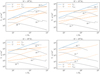 |
Fig. D.3. Radial distributions of Σ−, ΣA, Σ+, and Σadv for different masses of central SMBHs (see Eqs. (8)). Also shown is the stationary distribution Σstat (grey lines) for different Ṁ (in ṀEdd units) for αcold = 0.01 (see description in Sect. 3.1 and Appendix D). Minimum critical Σ− = ΣA ∼ 7 × 10⁴ g cm−2 for 106 − 108 M⊙ SMBH. |
Appendix E: Magnetic Prandtl number
The magnetic Prandtl number is the ratio of momentum diffusivity (i.e. microscopic kinematic coefficient of viscosity ν) to the magnetic diffusivity νm:
 (E.1)
(E.1)
In terms of the Reynolds number Re and magnetic Reynolds number Rem, defined as Re =VL/ν and Rem = VL/νm, where V and L represent some reference velocity and length, respectively, Prm = Rem/Re.
The processes of momentum exchange between the particles define the viscosity in the medium. Collisions of neutrals-neutrals, ion-neutrals, electron-neutrals are considered below, as well as collisions between photons and electrons (scattering). For simplicity, in the formulas below, we assume the pure hydrogen plasma and substitute the charge Z = 1 and ni = ne, but to calculate the electron volume density ne for Fig. 9 we use the mean number of free electrons per nucleon 1/μe = ne mp/ρ, as provided by the EOS-MESA module for solar abundances, called from ALPHADISC (see Appendix A). Hydrogen atom density is nH ≈ ((1 + X)/2 − 1/μe)ρ/mp, where X = 0.7 and the maximum number of free electrons per nucleon is (1 + X)/2.
We assume the same temperature for all species and ignore the magnetic field. For such plasma, the viscosity of electrons can be ignored (Zhdanov 2002), η = ηi + ηH. Approximately, we calculated the total kinematic viscosity as the sum
 (E.2)
(E.2)
where the radiation viscosity is (Mihalas & Mihalas 1984):
 (E.3)
(E.3)
where arad ≈ 7.566 × 10⁻¹⁵ g cm−1 s−2 T−4 is the radiation density constant and κ is the Rosseland opacity [cm2g−1], which we calculate using the EOS-MESA module of ALPHADISC.
We note that the resulting increase of Prm(ρ, T) at high temperature (see Fig. 9) is largely determined by the radiation viscosity (see also Potter & Balbus 2017). At the same time, it is important to recognise that Eq. (E.3) requires more consideration. On the microscopic scale, where the material viscosity works, the radiation cannot be treated in the diffusion approximation, under which the shear viscosity is derived (E.3) (Agol & Krolik 1998; Clouët & Soulard 2021). Nevertheless, the radiation reaction forces or bulk viscosity still work to dampen the velocity fluctuations and lower the Reynolds number Re. In the end, this leads to an increase in the Prandtl number (Jiang et al. 2013; Blaes 2014).
Formulae below are needed to describe not-fully ionised regimes when the Spitzer formulae do not apply. Including only the ionic viscosity in (E.2) and only the ee/ei resistivity in (E.7), we get Prm consistent with the expressions used in, for instance, Balbus & Henri (2008).
For the viscosity of partially ionised matter, we use expressions (4) and (7) for the ionic and atom viscosity from Vranjes (2014),
 (E.4)
(E.4)
where the collision times τcol, with the subscript i or H, are combinations of specific collision times between ions and H atoms (in the approximation of collisions of hard spheres or Coulomb interactions, see Zhdanov 2002, Sect. 5.1),
 (E.5)
(E.5)
and the dimensionless coefficients ξ lie in the interval 1−2 (see expressions E.12 below).
The magnetic diffusivity νm is related to the electrical conductivity σ as νm ≡ c2/(4πσ) (in CGS units, used by us, while νm = 1/(μ0σ) in SI), where the electrical conductivity σ (inverse resistivity) in the ionised plasma is (Spitzer 1962; Huba 2013)
 (E.6)
(E.6)
where  is the collision frequency of electrons.
We consider that the total magnetic diffusivity results from three types of collisions, electron-ion (ei), electron-electron (ee), and electron-neutral (eH):
 (E.7)
(E.7)
Here the specific collision times are presented below.
E.1. Collision coefficients
For the Lorentzian gas (collisions between electrons and protons only), the collision frequency is (Huba 2013)
 (E.8)
(E.8)
A modification taking into consideration electron-electron collisions yields the value  (Spitzer 1962).
The collision frequency between ions is (Huba 2013)
 (E.9)
(E.9)
The Coulomb logarithms λii = λei ∼ 5 for ne ∼ 1016cm−3 and T ∼ 104 K (Huba 2013).
General expression for the collision frequency of particles ‘x’ (electrons e, ions i, or atoms H) by the neutral hydrogen atoms is
 (E.10)
where we took as a rough upper estimate σs = 5 × 10⁻¹⁵ cm2 for each of the cross-sections σse|H, σsp|H, and σsH|H (see Huba (2013), the section on weakly ionised plasma, and Vranjes & Krstic (2013)). Further, for (E.5) we need τHp, which is found from the momentum conservation:
 (E.11)
In the scope of the mentioned assumptions (no magnetic field, single temperature, collisions of hard spheres or Coulomb interactions), the dimensionless coefficients ξ entering the expressions for the viscosity (E.4) can be calculated as follows (Sect. 7.1 of Zhdanov 2002; Vranjes 2014):
 (E.12)
All Tables
Peak accretion rate, characteristic duration, and mass involved in giant flares.
All Figures
|
Fig. 1. General S-curve at some radius in accretion disc. The limit cycle instability is shown schematically: on the lower branch the mass accumulates, on the upper branch the mass flows out of a ring. |
| In the text | |
|
Fig. 2. S-curves at different radii r1 < r2 < r3, shown schematically for ionisation instability. When the accretion rate is very low, the whole disc is stable and cold (the bottom line on the plot). If the surface density exceeds the critical value at the innermost radius r1, a heating wave, indicated by arrows, starts outwards, potentially reaching r3. |
| In the text | |
|
Fig. 3. Equilibrium curves for discs around stellar-mass BH (left panel) and SMBH (right panel). In each panel, the ξ-curves are constructed for two values of the turbulent parameter α: 0.1 and 0.01. The solid lines are calculated by ALPHADISC and their upper dotted tails correspond to Prad > Pgas. Analytic relations in the radiation-pressure regime (A zone, dashed, ∝Σ−1) and the advective regime (dash-dotted, ∝Σ) are calculated using Eqs. (B.5) and (B.4), respectively. The dots mark critical points for the geometrically thin states: the minimum and the maximum surface density, Σ+ and ΣA, in the ionised state and the maximum surface density Σ− in the recombined state The arrows schematically show the direction of ring heating due to ionisation instability. At the same time, α increases. |
| In the text | |
|
Fig. 4. S-curves for 107 M⊙ at r = 100 RS for two values of turbulent parameter αcold = 0.01 (blue) and αhot = 0.1 (orange). The branches ‘A-zone’ and ‘Advection’ were calculated using the code from Lipunova (1999). The accretion rate in absolute units shown on the left axis and in the Eddington rates (1), on the right (upper panel). Temperature Tc in the symmetry plane (middle panel). The dashed line shows the S-curve for αcold without convection. Relative semi-thickness z/r (bottom panel). |
| In the text | |
|
Fig. 5. Critical values of surface density (8) for M = 107 M⊙. The viscous parameter is αcold = 0.01 for Σ− (blue line) and αhot = 0.1 in all other dependencies (orange lines). The relations ΣA and ΣA′ show the results of different codes (see Sect. 3.1). |
| In the text | |
|
Fig. 6. Quasi-stationary surface density Σstat(r) for M = 107 M⊙ and α = αcold at several values of Ṁ, indicated in the graphs in units of ṀEdd (upper panel). Radial distributions of the critical points Σ+ for αhot and Σ− for αcold together with the stationary distributions (middle panel). The latter are shown only for Σstat < Σ−. Superimposed are the radial dependencies of the critical points ΣA and Σadv for αhot (bottom panel). In all panels, αcold = 0.01 (blue) and αhot = 0.1 (orange). The curves are plotted starting from 5RS. |
| In the text | |
|
Fig. 7. Accretion rate vs truncation radius of thin disc before giant flare. The predicted dependence between the accretion rate and the ADAF outer boundary (9) is also shown. The crosses mark the radius constraint due to self-gravity following (10). The transparent dashed style indicates the Rtrunc region excluded from further analysis. |
| In the text | |
|
Fig. 8. Outburst properties for normal (black) and giant flares (blue and orange) vs. inner truncation radius of quiescent geometrically thin disc. Peak accretion rate (13) (upper left); Characteristic times, calculated using (11) for the flare evolution before the peak and (5) for the characteristic flare duration (upper right); Inner disc accretion rate before the flare (bottom left); Mass involved in a flare (bottom right). The blue curves show the upper limit, obtained if the disc is heated to the radius Rout,max. The orange curves represent the lower limit following assumption Rout = Rtrunc + z0 (see Sect. 4). |
| In the text | |
|
Fig. 9. Magnetic Prandtl number calculated for disc around M = 107 M⊙ for α = 0.1 and 0.01 and radii 10 and 300 RS. The dots mark the locations of the critical surface densities Σ−. |
| In the text | |
|
Fig. 10. Disc mass (12) involved in giant flare vs viscosity time (5). The dots mark the values corresponding to the ADAF truncation radius (9), shown in Fig. 7. |
| In the text | |
|
Fig. 11. Truncation radii of thin discs and SMBH masses allowing giant flares (hatched area). The upper boundary corresponds to self-gravitation instability radius Rsg. Also shown are the circularisation radii Rcirc for stars of 1, 10, and 20 M⊙. |
| In the text | |
|
Fig. D.1. Analytic solutions for accretion rate evolution in disc without outflow with fixed z0/r (l = 1/3). At late times, the evolution is exponential in the disc with the constant outer radius (orange; Lipunova 2015) and power law, when the outer radius is expanding (blue; Lynden-Bell & Pringle 1974) For the both solutions, the mass is Mflare = 4M⊙ and initial ring radius Rout = 90 RS, which roughly correspond to the minimum flare in a disc around 107 M⊙ SMBH in Table 1. |
| In the text | |
|
Fig. D.2. Outburst parameters for giant flares (coloured areas) and normal flares (dotted lines) vs inner truncation radius of quiescent geometrically thin disc. From top to bottom, from left to right: Mass involved in a flare (14), estimated peak accretion rate (13), characteristic flare duration (5), and rise time (11). The upper boundaries of the coloured areas correspond to the case when the disc is heated to the radius Rout,max, the lower boundaries to the conservative assumption Rout = Rtrunc + z0 (see Sect. 4). The lower grey line illustrates the limits for intermediate masses. For 109 M⊙, ionisation instability always ignites a giant flare. |
| In the text | |
|
Fig. D.3. Radial distributions of Σ−, ΣA, Σ+, and Σadv for different masses of central SMBHs (see Eqs. (8)). Also shown is the stationary distribution Σstat (grey lines) for different Ṁ (in ṀEdd units) for αcold = 0.01 (see description in Sect. 3.1 and Appendix D). Minimum critical Σ− = ΣA ∼ 7 × 10⁴ g cm−2 for 106 − 108 M⊙ SMBH. |
| In the text | |
Current usage metrics show cumulative count of Article Views (full-text article views including HTML views, PDF and ePub downloads, according to the available data) and Abstracts Views on Vision4Press platform.
Data correspond to usage on the plateform after 2015. The current usage metrics is available 48-96 hours after online publication and is updated daily on week days.
Initial download of the metrics may take a while.