| Issue |
A&A
Volume 700, August 2025
|
|
|---|---|---|
| Article Number | A222 | |
| Number of page(s) | 30 | |
| Section | Planets, planetary systems, and small bodies | |
| DOI | https://doi.org/10.1051/0004-6361/202452513 | |
| Published online | 19 August 2025 | |
Characterizing planetary systems with SPIRou: Detection of a sub-Neptune in a 6-day period orbit around the M dwarf Gl 410★
1
Univ. Grenoble Alpes, CNRS, IPAG,
38000
Grenoble,
France
2
Univ. de Toulouse, CNRS, IRAP,
14 avenue Belin,
31400
Toulouse,
France
3
SUPA School of Physics and Astronomy, University of St Andrews,
North Haugh,
St Andrews
KY16 9SS,
UK
4
Aix Marseille Université, CNRS, CNES, Institut Origines, LAM,
Marseille,
France
5
Trottier Institute for Research on Exoplanets, Université de Montréal, Département de Physique,
C.P. 6128 Succ. Centre-ville,
Montréal,
QC
H3C 3J7,
Canada
6
Observatoire du Mont-Mégantic, Université de Montréal, Département de Physique,
C.P. 6128 Succ. Centre-ville,
Montréal,
QC
H3C 3J7,
Canada
7
Université Côte d’Azur, Observatoire de la Côte d’Azur, CNRS, Laboratoire
Lagrange,
France
8
Planétarium de Montréal, Espace pour la Vie,
4801 av. Pierre-de Coubertin,
Montréal,
Québec,
Canada
9
Instituto Tecnolόgico de Buenos Aires (ITBA),
Buenos Aires
C1437,
Argentina
10
International Center for Advanced Studies and ICIFI (CONICET), ECyT-UNSAM, Campus Miguelete,
25 de Mayo y Francia,
1650
Buenos Aires,
Argentina
11
Laboratόrio Nacional de Astrofísica,
Rua Estados Unidos 154,
37504-364,
Itajubá,
MG,
Brazil
12
Institut d’astrophysique de Paris, CNRS, UMR 7095, Sorbonne Université,
98 bis bd Arago,
75014
Paris,
France
13
Canada France Hawaii Telescope Corporation (CFHT), UAR2208 CNRS-INSU,
65-1238 Mamalahoa Hwy,
Kamuela,
HI
96743,
USA
14
Université de Montpellier, CNRS, LUPM,
34095
Montpellier,
France
15
Max-Planck-Institut für Astronomie,
Königstuhl 17,
69117
Heidelberg,
Germany
16
Center for Astrophysics, Harvard & Smithsonian,
60 Garden Street,
Cambridge,
MA
02138,
USA
17
Dep. de Física, Univ. Federal do Rio Grande do Norte – UFRN,
Natal,
RN
59078-970,
Brazil
18
Department of Physics & Astronomy, McMaster University,
1280 Main St West,
Hamilton,
ON
L8S 4L8,
Canada
19
Departamento de Matemática y Física Aplicadas, Universidad Catόlica de la Santísima Conceptiόn,
Alonso de Rivera
2850
Conceptiόn,
Chile
20
Observatoire Astronomique de l’Université de Genève,
Chemin Pegasi 51b,
1290
Versoix,
Switzerland
21
Space sciences, Technologies and Astrophysics Research (STAR) Institute, Université de Liège,
Allée du Six-Août 19C,
4000
Liège,
Belgium
★★ Corresponding author: This email address is being protected from spambots. You need JavaScript enabled to view it.
Received:
7
October
2024
Accepted:
4
April
2025
Abstract
Context. The search for exoplanets around nearby M dwarfs represents a crucial milestone in the census of planetary systems in the vicinity of our Solar System.
Aims. Since 2018 our team has been conducting a blind search program for planets around nearby M dwarfs with the near-IR spectro-polarimeter and velocimeter SPIRou at the Canada-France-Hawaii Telescope and with the optical velocimeter SOPHIE at the Haute-Provence Observatory in France. The aim of this paper is to present our results on Gl 410, a 0.55 M⊙ 480 ± 150 Myr old active M dwarf distant 12 pc.
Methods. We searched for planetary companions using radial velocities (RVs). We used the line-by-line (LBL) technique to measure the RVs with SPIRou and the template matching method with SOPHIE. Three different methods were employed, two based on principal component analysis (PCA), to clean the SPIRou RVs for systematics. We applied Gaussian processes (GP) modeling to correct the SOPHIE RVs for stellar activity. The ℓ1 and apodized sine periodogram analysis was used to search for planetary signals in the SPIRou data taking into account activity indicators. We analyzed TESS data and searched for planetary transits.
Results. We report the detection of a M sin(i) = 8.4 ± 1.3 M⊕ sub-Neptune planet at a period of 6.020 ± 0.004 days in circular orbit with SPIRou. The same signal, although with lower significance, was also retrieved in the SOPHIE RV data after correction for activity using a GP trained on SPIRou’s longitudinal magnetic field (Bℓ) measurements. The TESS data indicate that the planet is not transiting. Within the SPIRou wPCA RVs, we find tentative evidence for two additional planetary signals at 2.99 and 18.7 days.
Conclusions. Infrared RVs are a powerful method to detect extrasolar planets around active M dwarfs. Care should be taken, however, to correct or filter systematics generated by residuals of the telluric correction or small structures in the detector plane. The LBL technique combined with PCA offers a promising way to reach this objective. Further monitoring of Gl 410 is necessary.
Key words: methods: observational / techniques: radial velocities / techniques: spectroscopic / planets and satellites: detection / planetary systems
Based on observations obtained with the spectropolarimeter SPIRou at the Canada-France-Hawaii Telescope (CFHT).
© The Authors 2025
 Open Access article, published by EDP Sciences, under the terms of the Creative Commons Attribution License (https://creativecommons.org/licenses/by/4.0), which permits unrestricted use, distribution, and reproduction in any medium, provided the original work is properly cited.
This article is published in open access under the Subscribe to Open model. This email address is being protected from spambots. You need JavaScript enabled to view it. to support open access publication.
1 Introduction
One of the most interesting open questions in current Astronomy is the census of extrasolar planets in the vicinity of the Solar System. The identification of the closest extrasolar planetary systems is a crucial milestone for the study of exoplanet atmospheres and biomarkers using future instrumentation combining high-dispersion spectroscopy with high contrast imaging (e.g., Kasper et al. 2021; Chauvin 2024). As the most stars in the Galaxy, and thus in the Solar neighbourhood, are low-mass stars (M ≤ 0.5 M⊙), in recent years, there has been growing interest in extending the planet search effort from solar-like stars to M dwarfs.
Radial velocity (RV; Bonfils et al. 2013; Pinamonti et al. 2022; Mignon et al. 2025) and transit surveys (Dressing & Charbonneau 2013, 2015; Mulders et al. 2015; Hsu et al. 2020; Ment & Charbonneau 2023) have revealed that a large fraction of M dwarfs, if not all, host a planetary system, and these surveys have provided strong evidence supporting the hypothesis that the rocky planet ratio per star is indeed larger than one. Extrapolating the results from field stars to our stellar vicinity is extremely encouraging, as it suggests that it is highly likely that a large fraction of nearby M dwarfs host multi-planetary systems. Nearby stars are distributed all over the sky at random orientations. A small fraction of sources are expected to present planets in transit. Missions such as TESS, and in the future, PLATO will detect a significant fraction of those transiting planets. Nevertheless, to establish the planetary systems census of our closest stellar neighbors, techniques such as astrometry or RVs need to be used in addition to transits.
Surveys for planetary systems around nearby bright M dwarfs with high-precision velocimeters have been carried so far mainly in the optical domain. Recently, the search using RVs has been extended to the near-infrared (IR) domain with the start of operations of new velocimeters such as HPF1 (Mahadevan et al. 2014), CARMENES2 (Quirrenbach et al. 2018), SPIRou3 (Donati et al. 2020) and NIRPS4 (Bouchy et al. 2017). High-precision IR RVs enable the exploration of lower mass stars, which are sometimes inaccessible for precise RV work in the optical due to their faintness. Furthermore, IR RVs have the potential of being less affected by stellar activity than optical RVs, especially for highly or moderately active stars (e.g., Carmona et al. 2023).
With more than two thousand low-mass M dwarfs in the 25 pc vicinity, the effort to monitor all of these objects is colossal. Thanks to large programs with the near-IR spectra-polarimeter and velocimeter SPIRou at CFHT (the SPIRou Legacy Survey, the SPICE large program) and a series of PI SPIRou follow-up programs, our team has been monitoring a select sub-sample of around 60 nearby M dwarfs. At the time of writing, we have obtained more than 100 visits per source for around 45 of them.
In this paper, we report the detection of a sub-Neptune mass planet in a 6-day period around the nearby (~ 12 pc) 0.55 M⊙ 480 Myr old M dwarf Gl 410 with SPIRou, and the tentative detection of two additional planetary signals at 2.99 and 18.7 days. We complement our near-IR data set with quasi simultaneous optical observations obtained with the velocimeter SOPHIE5. The paper is organized as follows. We describe the physical properties of Gl 410 in Sect. 2. Then, in Sect. 3, we present the details of the optical and infrared RV measurements. In Sect. 4, we analyze our RV measurements and test the robustness of the planet detection. In Sect. 5, we search for the 6-day period signal detected with SPIRou in the SOPHIE data using Gaussian processes (GP) activity filtering techniques. We derive the orbital and physical properties of the detected 6.02 day planet using Markov chain Monte Carlo (MCMC) techniques in Sect. 6. In Sect. 7, we investigate the presence of other planetary signals within the SPIRou wPCA RVs. In Sect. 8, we present TESS observations of Gl 410 and investigate whether Gl 410b is transiting. Finally, we discuss our findings in Sect. 9, and in Sect. 10, we provide our conclusions.
2 GI410
We summarize the basic physical properties of Gl 410 (DS Leo, HD 95650) in Table 1. Gl 410 is a nearby star located at a distance of  pc (Gaia DR3, Bailer-Jones et al. 2021; Gaia Collaboration 2023). It has a spectral type M1.0V and a mass of 0.55 ± 0.02 M⊙ (Cristofari et al. 2022). Gl 410 is known to exhibit cyclic photometric variability in the optical with periods of about 14 days, which is interpreted as being caused by rotational modulation of stellar spots (Fekel & Henry 2000). The rotational period of Gl 410 has been tightly constrained using spectropolarimetry observations in the optical with ESPaDOnS, NARVAL, and HARPS (Donati et al. 2008; Hébrard et al. 2016), and in the near-IR with SPIRou (Fouqué et al. 2023; Donati et al. 2023). The latest estimation of Prot is of 13.91 ± 0.09 days (Donati et al. 2023). Gl 410 displays surface differential rotation with periods at the equator and pole of 13.37 ± 0.86 and 14.96 ± 1.25 days, respectively (Hébrard et al. 2016). Based on gyrochronologly Fouqué et al. (2023) derived an age of 0.89 ± 0.1 Gyr for Gl 410. However, there is the possibility that Gl 410 is in fact younger. In Appendix A in the Appendix, we provide further details. We find that the empirical rotation-temperature sequences in clusters of known ages indicate that Gl 410 is 480 ± 150 Myr, thus placing it among the youngest stars in the solar neighborhood (Silva Aguirre et al. 2018; Chen et al. 2020) and suggesting that Gl 410 might be related to the Ursa Major (UMA) cluster which is approximately 400 Myr old.
Based on SPIRou observations, Cristofari et al. (2023) measured an average magnetic small scale field strength <B> of 0.71 ± 0.03 kG for Gl 410. Together with the M dwarfs GJ 1289 and GJ 1286, Gl 410 is one of the most magnetic stars among the M dwarfs studied in the <B> surveys of Reiners et al. (2022) and Cristofari et al. (2023). The magnetic activity of Gl 410 is further indicated by the presence of Hα emission in the optical spectra. Gl 410 is part of the top one-third of the sample in terms of Hα emission strength among the 331 M stars surveyed by Schöfer et al. (2019).
Zeeman Doppler imaging (ZDI) investigations by Donati et al. (2008), Hébrard et al. (2016), and Bellotti et al. (2024) have shown that the large-scale magnetic field of Gl 410 rapidly evolves both in strength and in topology. Between 2007 and 2008, the field had a predominantly toroidal geometry with an average strength of 100 G (Donati et al. 2008). In 2014, the field remained mostly toroidal with axisymmetric geometry, but the average field strength decreased to 60 G (Hébrard et al. 2016). In 2020b to 2021a the magnetic energy became almost equally distributed between the poloidal and the toroidal components and the average field strength decreased to 44 G (Bellotti et al. 2024). In the latest measurements from 2021b to 2022a, the poloidal component became much stronger than the toroidal component with 73% of the magnetic energy, and the average field strength further decreased to 18 G (Bellotti et al. 2024).
Stellar properties of Gl 410.
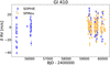 |
Fig. 1 Radial velocity time series measured in the optical with SOPHIE (blue dots) and in the near-IR with SPIRou (orange dots). |
3 Observations
3.1 SOPHIE
Gl 410 was observed during two periods 9 years apart with the high-resolution optical velocimeter SOPHIE (Perruchot et al. 2008; Bouchy et al. 2013) at the 1.93 m Telescope of the Haute-Provence Observatory in the South of France. The first period with 45 visits was observed from March 14, 2010, to June 14, 2012. A second observation period was planned to coincide with the SPIRou observations, with 58 visits performed from January 26, 2021, to March 04, 2023. Spectra were reduced using SOPHIE’s data reduction system (Bouchy et al. 2009; Heidari 2022). The RV measurements were obtained using a template-matching technique implemented in the code NAIRA (Astudillo-Defru et al. 2015), which has been adapted for SOPHIE (Hobson et al. 2018). The SOPHIE RV measurements are given in Table 2 (the full table is available at the CDS). In Table 4, we provide a summary of the properties of the RV time series. Figure 1 displays the median subtracted SOPHIE RV data.
3.2 SPIRou
Gl 410 was observed with the near-IR velocimeter and Polarimeter SPIRou (Donati et al. 2020), mounted at the Canada-France-Hawaii Telescope atop Mauna-Kea during 156 visits from April 2018 to July 2023. Data were obtained in the context of the SPIRou’s commissioning in 2018, the SPIRou Legacy Survey from 2019 to 2022A, and a series of PI follow-program programs (PI. Carmona, PI. Artigau) in 2022B, 2023A and 2023B. Nightly SPIRou observations typically consist of a Stokes V sequence of four exposures, each taken with different positions of the Fresnel rhombs inside the Polarimeter. The combination of the channel A and channel Β of the four sub-exposures enables the recovery of the Stokes V (and Stokes I) spectra for magnetic field analysis. For each science observation, a simultaneous Fabry-Pérot exposure was obtained in the calibration channel C. In the context of the RV analysis, we used the combined extraction of the science channels A and Β and each sub-exposure of the Stokes V sequence was treated independently.
For the RV analysis, we used the data reduced using the APER0 (Cook et al. 2022) pipeline version v07275 installed at the SPIRou Data Centre hosted at the Laboratoire d’Astrophysique de Marseille. We note that APER0 extracts the combined science channel A and channel Β spectra, performs the wavelength calibration using nightly observations of the Uranium-Neon lamp and Fabry-Pérot exposures, and conducts the telluric correction. The telluric correction uses a combination of an atmospheric absorption model generated by TAPAS (Bertaux et al. 2014), an empirical template of the star deduced from observations at different barycentric earth radial velocity (BERV) and a library of nightly observations of telluric standard stars taken since the commissioning of the instrument in 2018. Further details on the telluric correction are given in Artigau et al. (2014), Cook et al. (2022) and Artigau et al., (in prep.). Individual RV measurements were obtained using the LBL technique (Artigau et al. 2022), and they were corrected by the BERV and the drift of the Fabry-Pérot at each exposure. A further correction for the instrumental RV zero point was done using a GP model based on observations of a sample of RV standard stars observed by SPIRou (Cadieux et al. 2022). The SPIRou LBL RV measurements are given in Table 3 (full table available at the CDS).
For analysis of the stellar activity, we used the simultaneous longitudinal magnetic (Bℓ) field measurements obtained with the Libre-ESpRIT pipeline6 previously published in Donati et al. (2023).
SOPHIE RV measurements of Gl 410.
3.3 TESS
The Transit Exoplanet Survey (TESS; Ricker et al. 2014) observed Gl 410 (TIC 97488127) with a two-minute cadence during Sector 22, from February 18 to March 18, 2020. We obtained the Presearch Data Conditioning (PDC) flux time series (Smith et al. 2012; Stumpe et al. 2012, 2014) processed by the TESS Science Processing Operations Center (Jenkins et al. 2016) from the Mikulski Archive for Space Telescopes (MAST)7.
4 Radial velocity analysis
For the RV analysis, we used Generalized Lomb–Scargle (GLS) periodograms (Zechmeister & Kürs ter 2009). To determine the false alarm probability levels (FAP), we used two methods. For peaks with a significance lower than 10–5 and the 10%, 1%, and 0.1% FAP levels in the periodograms, we used a bootstrap algorithm with 105 iterations. The method consists in generating a time series with dates equal to the real series of measurements, but assigning to each of them a RV measurement chosen randomly from the original data series. We labeled these FAP levels FAPbootstrap. For peaks with a significance higher than 10–5 (i.e., inferior to 1/number of boostrap iterations), we used the GLS FAP analytical implementation of the package pyAstronomy (Czesla et al. 2019). We labeled these FAP levels FAPanaiyticai.
SPIRou LBL and Wapiti RV measurements of Gl 410.
SOPHIE RV time series and periodogram. properties.
4.1 SOPHIE radial velocities
We achieved with SOPHIE an average RV precision per measurement of 2.4 m s–1 and an rms of 13.9 m s–1 in the full time series. Figure 2 displays the GLS periodograms obtained for the full data set, the 2010–2012, and 2021–2023 periods, respectively. Table 4 summarizes the properties of the time series and the strongest peak in the periodogram.
The full data set displays a peak at P = 6.92 days with an FAPbootstrap of 4.0 × 10⁻⁴. This peak corresponds to the P/2 harmonic of the stellar rotation period of P = 13.91 days (Donati et al. 2023). Apart from the 1 day alias, there are no other peaks in the full data set periodogram. No signal is observed at the stellar rotation period. The 2010–2012 period shows no significant periodicities. A broad peak is observed close to P = 6.99 days but its significance is low (FAPbootstrap = 0.2). In the 2021–2023 period, a peak at P = 6.91 days appears at an FAPbootstrap level of 3.8 × 10⁻³. Except for the 1 day alias, no peaks are present in the periodogram with a significance below an FAPbootstrap = 10%.
In summary, in the raw SOPHIE RV data, there is a signal at P = 6.9 days, but it is most likely related to the stellar rotation.
4.2 SPIRou radial velocities
With SPIRou, we achieved an average RV precision per measurement of 2.3 m s–1 and an rms of 9.1 m s–1 in the full LBL time series. We display in the left panels of Fig. 3, the SPIRou LBL RV measurements as a function of time and their GLS peri-odogram. The periodogram displays a peak at P = 6.02 days with a FAPbootstrap level of 2.2%. No peaks are observed at the rotational period of the star nor its harmonics. The SPIRou LBL RV measurements are listed in Table 3 (the full table is available at the CDS). A summary of the properties of the LBL RV time series is given in Table 6.
Due to the reflex motion of the Earth in its orbit (i.e., the BERV), observations acquired at different moments of the year have different velocity shifts with respect to the center of telluric absorption lines. If a star has an intrinsic average systemic velocity Vsys with respect to the Sun, the total velocity Vtot of the star at the time of the observations is given by
 (1)
(1)
In the near-IR, the telluric absorption lines are abundant, thus the stellar photospheric absorption lines are affected by tel-lurics. The first effect of telluric absorption is the deformation of the photospheric line profiles. After telluric correction, residuals from atmospheric lines, at a much lower level than original, may remain, and even for a perfect correction, the noise is higher in the affected velocity channels. The moment the stellar spectra is most affected by tellurics is when the atmospheric absorption is at the core of the stellar photospheric lines, that is when Vtot is between –10 and +10 km s–1. In other words, this is when the absorption lines of chemical species common to the Earth’s atmosphere and the stellar photosphere (e.g., H2O, CO) are on the top of each other, particularly in regions where the optical depth of the atmosphere is the greatest.
We have color-coded in Fig. 3 the RV measurements based Vtot. We display the observations obtained when |Vtot| > 10 km s–1 in blue and the observations taken when |Vtot| < 10 km s–1 in red. The telluric correction of APER0 is good, the LBL algorithm is efficient at filtering outliers, and the zero-point correction in time and BERV space further corrects residuals of telluric lines. However, as shown in Fig. 3, at the meter per second RV precision level, the systematic noise of tellurics is evident. Fig. 3 shows that a large fraction of the outliers in the RV time series are in red. The effect of telluric lines becomes evident when the RV time series is plotted as a function of Vtot (see Fig. 3). The systematics due to the telluric absorption can be seen, as an up and down correlated-noise pattern.
If the RV time series is filtered from the data-points taken at |Vtot| < 10 km s–1 (i.e., the red points in Fig. 3), the rms of the time series (see Table 6), improves: from 9.1 m s–1 for the full time series to 6.5 m s–1 for the filtered time series. If the periodogram is made only with observations taken at |Vtot| > 10 km s–1, we not only recover the peak at 6.02 days detected in the full time series, but its significance increases from an FAPbootstrap = 0.022 in the full time series to FAPanalytical = 1.4 ×10⁻⁸ in the filtered time series. The case of Gl 410 dramatically shows the effect that telluric residuals can have adding RV noise, ultimately blurring a planet detection.
Filtering data-points taken at |Vtot| < 10 km s–1 is a robust and fast way of finding promising planet candidate signals. However, apart the obvious fact that this approach takes out a large of number data points (39 measurements), it also has the limitation that it can boost the power at certain frequencies because specific and periodic times are missing in the time sampling. The RV systematics and correlated noise generated both by telluric residuals and detector-based glitches and imperfections can be corrected. The LBL framework produces a 2D data set, a time series for each of the thousands of LBL line measurements. In this 2D data set, data-driven techniques such as principal component analysis (PCA) can be employed to further filter, mitigate, and correct systematic noise in the RV measurements.
In the context of the SPIRou collaboration, two PCA-based LBL RV correcting algorithms have been developed: Wapiti (Ould-Elhkim et al. 2023) and a weighted PCA method (wPCA; Artigau et al., in prep). We refer to those papers for details on each methodology. The main difference between these two approaches is that Wapiti performs a PCA in the stellar velocity space, whereas in the second method, the PCA is applied in the detector pixel space (inspired on Cretignier et al. 2023). The Wapiti and wPCA RV measurements are given in Tables 3 and 5, respectively (both tables are available at the CDS). We reanalyzed the RV data of Gl 410 with both of these methods. In the central and right panels of Fig. 3, we display the RV measurements and GLS periodograms obtained with wPCA and Wapiti. In Table 6, we present the summary of the properties of the RV time series.
Figure 3 illustrates how wPCA and Wapiti correct for the systematic noise at |Vtot| < 10 km s–1. The rms of the full time series decreases from 9.1 m s–1 in the raw LBL to 6.8 m s–1 with wPCA and 6.3 m s–1 with Wapiti. The rms of the points at |Vtot| < 10 km s–1 (red dots in Fig. 3) decreases from 14.3 m s–1 in the raw LBL, to 7.1 m s–1 with wPCA and 8.3 m s–1 with Wapiti. We also observed that the peak at P = 6.02 days becomes stronger in the full time series and that it reaches an FAPbootstrap level of 3.5 × 10⁻⁶. Furthermore in the wPCA RV data, a new peak at P = 18.76 days with an FAPbootstrap level of 1.6% becomes visible. A peak at 18.73 days is also present in the Wapiti time series, however, it has a negligible significance (FAPbootstrap = 80%).
In summary, the SPIRou RV data shows a clear periodic signal at a P = 6.02 days. The signal is not a harmonic or alias of the rotation period. There is evidence for a second, tentative, candidate signal at P = 18.7 days.
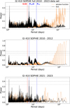 |
Fig. 2 Generalized Lomb-Scargle Periodograms of the SOPHIE RV time series for the full 2010–2023 data set (top), the 2010–2012 period (middle), and the 2021–2023 period (bottom). The location of the rotational period of Prot = 13.9 days and its Prot/2 harmonic are indicated with blue vertical lines. The position of P = 6.02 days is displayed with a red vertical line. The horizontal lines indicate the bootstrap calculated at 0.1%, 1%, and 10% FAP levels. The window function is shown with a light orange color. |
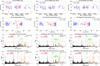 |
Fig. 3 SPIRou RV measurements as a function of time and GLS periodograms for the “raw” LBL measurements and the PCA corrected LBL measurements obtained with wPCA (Artigau et al., in prep) and Wapiti (Ould-Elhkim et al. 2023). Blue dots indicate the measurements taken at |Vtot| > 10 km s–1. Red dots are the measurements obtained when |Vtot| < 10 km s–1 (i.e., moment of the highest influence of the atmosphere on the stellar spectrum). In the periodograms, the gray horizontal lines indicate the bootstrap-calculated 10%, 1%, and 0.1% FAP levels. A summary of the statistics of the each of the time series is provided in Table 6. |
SPIRou LBL wPCA RV measurements of Gl 410.
SPIRou RV time series and GLS periodogram properties.
4.3 A test of robustness of the 6-day SPIRou signal
No periodicities were detected at 6.02 nor at 18.7 days in the activity indicators time series of SOPHIE and SPIRou (details are provided in Appendix B). We performed an additional test of robustness to exclude the possibility that the signal at 6 days is due to activity. If a candidate signal is due to a planet (and not activity), it is expected that as more RV data points are accumulated the significance of the detection increases, and this should not depend on the way the time-sampling of the measurements is performed.
Using the |Vtot| > 10 km s–1 SPIRou wPCA time series, we performed a test that consists in checking the evolution of the FAP level of the P = 6 days peak in 100 different randomly sampled time series. The construction of an RV time series starts by randomly selecting ten measurements, calculating the GLS periodogram, and measuring the FAP of the peak at P = 6 days. One randomly selected measurement is then included in the time series, the periodogram is recalculated, and the FAP of the peak at P = 6 days is measured. The procedure is repeated until the complete number of visits is reached for a time series. In this way, we constructed 100 independent evolutions of the FAP as a function of the number of measurements. This test implies the calculation of around twelve thousand FAPs. To keep the computation time short, we calculated the FAP level using the analytical approximation implemented in pyAstronomy (Czesla et al. 2019). The analytical FAPs are a factor of a few lower than the FAPs calculated using a bootstrap method.
The result of the test is displayed in Fig. 4. One can see that for all the time series, the FAP level of the P = 6 days peak decreases as the number of measurements increases. In Fig. 4, we include the plot of the FAP level in the chronological time series and the median FAP for each bin of number of measurements. The test indicates that the peak at P = 6 days in the periodogram is physical and that it does not depend on the sampling of the time series. This test supports the argument that the Ρ = 6 days peak in the periodogram is indeed of Keplerian origin.
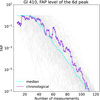 |
Fig. 4 Test on the change of the FAP level of the peak on the peri-odogram at 6 days as a function of the number of visits for 100 randomly selected time series. The FAP level of the Ρ = 6 days peak decreases as a function of the number of measurements, as expected for a planetary origin of the signal. The random time series were sampled from the |Vtot| > 10 km s–1 RV time series. The FAP level in this test was calculated using the analytical approximation implemented in pyAstronomy (Czesla et al. 2019). |
5 Stellar activity filtering of the SOPHIE radial velocities and search for the Gl 410b signal
As opposed to a signal due to activity, a Keplerian reflex motion caused by the presence of a planet is achromatic. There is a hint of the 6-day period signal in the SOPHIE RV data of Gl 410. If the SOPHIE and SPIRou RVs are plotted phase-folded, both data sets are consistent. However, the SOPHIE RVs have a much larger dispersion (14 m s–1) than the SPIRou RVs (7 m s–1). One interesting question is whether Gl 410b’s RV periodic signal could be retrieved in the SOPHIE data set if the RV jitter induced by stellar activity is corrected.
We tested two methods to search for the 6-day signal within the SOPHIE RV data. In the first method, the SOPHIE RVs time series is analyzed with a model that is the sum of a quasi-periodic GP and a Keplerian model. In the second method, we used the measurements of the longitudinal magnetic field (Bℓ) from SPIRou to inform a GP that is used to correct the SOPHIE RVs for activity jitter, and then we searched for the planet signal in the RV residuals.
5.1 Method 1: SOPHIE Gaussian process modeling using the SOPHIE radial velocity data alone
As the rotational period of Gl 410 is well constrained by spec-tropolarimetry, the SOPHIE RV data can be analyzed using a GP plus Keplerian model. The goal here is to determine what model is more probable between a model without a planet (i.e., only a GP) and a model with a GP plus a planet. To perform the analysis, we used RadVel (Fulton et al. 2018) and assumed a circular orbit. A Gaussian prior was used for the GP period, with center at 13.9 days and σ = 0.1 days, which corresponds to the stellar rotation period derived from the measurements of the longitudinal magnetic field Bℓ (Donati et al. 2023). Uniform priors were set for the planet period Pb (0 to 20 days), the planet semi-amplitude Kb (0 to 20 m s–1), the time of inferior conjunction T conjb (2459648.0 + 10 days), the GP amplitude A (0–75 m s–1), the GP decay time l (0–2000 days), the GP smoothing length Γ (0–2 days), and the uncorrelated noise σSOPHIE (0.0–10 m s–1).
Table 7 provides a summary of the small sample Akaike information criterion (AICc) tests comparing the models. The model with a GP model alone (i.e., without planet) was statistically “ruled out” by RadVel. In Table C.1 in the Appendix, we present the posterior distributions obtained for the model8. The Keplerian signal at Ρ = 6.02 days is retrieved in the model. This test provides independent evidence for the existence of the 6-day planet inside the SOPHIE RV data. In Sect. 6.3, we discuss the coherence of the Keplerian signals obtained with SPIRou and SOPHIE.
RadVel model comparison table for the GP plus Keplerian model on the SOPHIE RVs alone.
5.2 Method 2: SOPHIE Gaussian process modeling using SPIRou’s Bℓ as an activity proxy
In this second method, the search of the signal is done using a two-step approach. In step one, a quasi-periodic GP model is fit to the SPIRou’s longitudinal magnetic field (Bℓ) time series, and in step two, the posterior distribution of the hyper parameters (period, decay time, and smoothing length) of the Bℓ GP are used as prior for a quasi-periodic GP model of the SOPHIE RVs (other hyperparamers, such as In A, and In s, priors are taken as uniform). The aim of this method is to filter the SOPHIE RVs for activity using Bℓ as a proxy of the activity signal and search for the signal at 6 days in the residuals.
We used the SPIRou Bℓ measurements from Donati et al. (2023). In Appendix C, we describe the quasi-periodic GP model we used. In Fig. D.1, also in the Appendix, we display the MCMC corner plots of the Bℓ GP. We retrieved in our GP model of Bℓ a stellar rotational period of 13.93 ± 0.09 days, which is consistent with the previous determinations of the rotational period by Donati et al. (2023) and Fouqué et al. (2023). We modeled the SOPHIE RVs with the same quasi-periodic GP model and implementation used for Bℓ. We focused on the SOPHIE RVs from 2021 to 2023, as this period has the quasi-simultaneous SPIRou Bℓ measurements9. The prior and posterior distributions for the RV GP are given in Table C.1 in the Appendix. In Figure D.2, also in the Appendix, we show the MCMC corner plots of the RV GP model. Figure 5 summarizes the model results. The upper panel shows the GP model (in blue) and the SOPHIE RVs (black points). The middle panel displays the GP-corrected SOPHIE RVs. The lower panel shows the GLS periodogram of the GP-corrected SOPHIE RVs. After correcting for the activity jitter, the RV rms decreases from 12.7 m s–1 to 6.0 m s–1, and the GLS periodogram shows a clear and strong peak at Ρ = 6.02 days with a FAPbootstrap of 2.4 × 10⁻³. This period is the same as that obtained in the SPIRou RV measurements.
In Figure 6, we display the phase-folded SPIRou RV time series together with the SOPHIE GP-corrected RVs, while overlaying a Keplerian model fit with Κ = 5 m s–1 and Ρ = 6 days. The data of both instruments are compatible. This, provided us, one more time, with further arguments to support the idea that the periodic signal at 6 days detected with SPIRou indeed has a Keplerian origin.
We calculated a periodogram for the combined SPIRou (wPCA) and SOPHIE minus GP RV time series. It is shown in Fig. 7. The periodogram of the combined SPIRou and SOPHIE minus GP data set (black lines) is very similar to that of the wPCA SPIRou data alone (green lines). However, the addition of the SOPHIE minus GP RVs makes the FAP levels of the periodogram decrease to lower powers (we emphasize the difference between the horizontal gray and green lines in the plot). The significance of the peak at P = 6.02 days increases from an FAPanalytical = 3.5×10⁻⁶ in the wPCA SPIRou data alone to an FAPanalytical = 1.5×10⁻⁹ in the combined near-IR plus optical data set.
We find that the properties of the RV GP trained on Bℓ are different from those of the GP based on the RV data alone. The period of both GPs is the same, as we imposed in the priors the rotational period of the star. The amplitude of each GP is slightly different:  m s–1 for the GP based on the SOPHIE RVs alone and 12 ± 3 m s–1 for the GP trained on Bℓ. The decay time of each GPs is significantly different, from
  days from the GP based on the SOPHIE RVs alone to 60 ± 8 days from the GP informed on Bℓ. These differences in the GPs will produce different amplitudes of the recovered Keplerian signal. In Sect. 6, we discuss in detail the properties of the Keplerian signal retrieved in the SPIRou data. We show in Section 6, that the Kb recovered in the SOPHIE data set corrected with the GP using Bℓ as a proxy of activity is almost the same as the Kb derived from the SPIRou wPCA and Wapiti data sets. Our analysis suggests that a GP informed on Bℓ as proxy of activity provides a good correction for the stellar activity RV jitter in the optical.
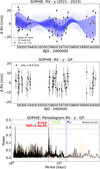 |
Fig. 5 Upper panel: SOPHIE RVs minus the RV offset γ (zoom-in of the period 2021–2023) together with the quasi-periodic GP model (blue lines) obtained using SPIRou’s Bγ GP posterior distributions of the period, decay time, and smoothing length as priors for the SOPHIE RVs GP. Middle panel: SOPHIEs RVs after correction of the RV offset and the GP. The rms of the RV time series decreases from 12.7 m s–1 to 6.0 m s–1 in the GP-corrected data. Lower panel: periodogram of the GP-corrected SOPHIE RVs. The peaks related to Prot/2 disappeared after GP correction. A peak at the period of 6.02 days (FAPbootstrap = 2.4 × 10⁻³), the same period found in the SPIRou RVs, is retrieved. Horizontal lines are the 10%, 1%, and 0.1% FAP levels (calculated using a bootstrap algorithm). |
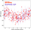 |
Fig. 6 Phase-folded SPIRou (wPCA) and GP-corrected (using Bℓ as an activity proxy) SOPHIE RV measurements. The model in gray is a circular Keplerian fit to the SPIRou data with Κ = 5 m s–1 and Ρ = 6 days. |
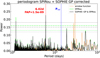 |
Fig. 7 Generalized Lomb-Scargle periodogram of the combined SPIRou (wPCA) and SOPHIE GP-corrected (using Bℓ as an activity proxy) RV measurements. The gray horizontal lines display the bootstrap-calculated FAP levels of 10%, 1%, and 0.1%. For comparison, we overplot in green the periodogram and FAP levels of the SPIRou data alone. The FAP of the 6-day period peak improves in the SOPHIE plus SPIRou time series with respect to the SPIRou data alone (see Fig. 3). |
6 Gl 410b physical properties
6.1 Gl 410b physical properties derived from the SPIRou radial velocities
We derived the Gl 410b planet candidate properties using RadVel. We calculated RadVel models for each of the SPIRou RV data sets: LBL |Vtot| > 10 km s–1, wPCA, and Wapiti. Models with circular and eccentric orbits were considered. In all models, we started performing a maximum-likelihood fit to define the prior centers of the fit manually and then we performed the MCMC model exploration. Uniform bounds priors were utilized for the planet’s period Pb (between 0 and 20 days, with the initial guess at 6 days); the planet’s semi-amplitude Kb (between 0 and 20 km s–1, with the initial guess 6 m s–1); the SPIRou uncorrelated noise σSPIRou (between 0 and 10 m s–1, with the initial guess 1 m s–1); and T conjb (2459648.0 ± 10 days and an initial guess of 2459648.0). The slope (dvdt) and the curvature (curv) were set to zero. We fed RadVel the median-subtracted RV points, and thus, the initial guess for the velocity zero-point was set to zero. The eccentricity was left to vary from zero to 0.99. We used a stellar mass of 0.55 ± 0.02 M⊙. The MCMC RadVel modeling used 50 walkers, 10000 steps, eight ensembles and a minimum autocorrelation factor of 40.
Table 8 shows the results of the RadVel AICc tests. In the |Vtot| > 10 km s–1 data, the circular orbit is “somewhat disfavored” with respect to the eccentric orbit. In the wPCA data, the eccentric solution is favored, but the circular orbit is “nearly indistinguishable” from the eccentric orbit. In the Wapiti data, the circular solution is favored, but the eccentric solution is “nearly indistinguishable” from the circular solution. The eccentricity distributions retrieved by RadVel are eb = 0.27 ± 0.14 for the |Vtot| > 10 km s–1 data, eb = 0.26 ± 0.17 for the wPCA data, and  for the Wapiti data. In all data sets, the eccentricity, eb, is constrained to be lower than 0.4. As the circular and eccentric orbits provide solutions that statistically are nearly indistinguishable and the center of the eccentricity distributions is below 2σ away fromzero, wefavoracircularorbitmodel. This model has a lower number of free parameters, and it provides a good description of the data.
Table 9 summarizes the retrieved orbital and planet parameters for the circular orbit model in each data set. Figure 8 displays the phase-folded SPIRou RVs together with the bestfit circular orbit model for each of the SPIRou RV reductions and the MCMC corner plots for the planet’s mass and semimajor axis. The RadVel models further confirm the detection of Gl 410b. As for all SPIRou data sets, the model without a planet is “ruled out”. Across all the SPIRou data sets and models the period of the planet converges to P = 6.02 days; thus, a semi-mayor axis of the planet, a, equal to 0.0531 au. The wPCA and Wapiti data sets give similar properties for the planet. The semi-amplitude retrieved in the LBL |Vtot| > 10 km s–1 data is larger, 5.3 ± 0.7 m s–1, which translates to a Mb sin(i) of 10.1 ± 1.3 M⊕.
We note that the PCA methods filtering the LBL data do in fact decrease the global dispersion of the all the RVs (not only those at |Vtot| < 10 km s–1). This is likely because of the diminution of the correlated noise and telluric correction residuals. However, the estimations of the planet mass with and without PCA correction methods are consistent within their 1σ error bar. As the wPCA displays the second peak in the periodogram, and the time series has the best correction of the |Vtot | < 10 km s–1 data, we favor the wPCA model. In the following, the wPCA circular orbital model is our baseline solution.
Taking the results altogether, the SPIRou RVs analysis indicate that the candidate planet Gl 410b has a M sin(i) of 8.4 ± 1.3 Earth masses, orbits at a distance of 0.0531 ± 0.0006 au from of its central star, with a period of P = 6.020 ± 0.004 days in a circular orbit. Gl 410b is a sub-Neptune planet.
RadVel model comparison table for the SPIRou RVs data sets (one-planet model).
Orbital parameters and physical properties of Gl 410b derived from the SPIRou RV data using a RadVel MCMC model of a planet in a circular orbit.
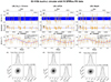 |
Fig. 8 Results of the RadVel MCMC Keplerian circular orbital model with one planet of the SPIRou RV time series. Each column represents the results for each set of data reductions: LBL at |Vtot| > 10 km s–1, wPCA, and Wapiti. Panel a shows the RV time series, panel b displays the residuals as a function of time, panel c plots the phase-folded RVs together with the best fit model (blue line), and the panel d displays the corner plots of Mb sin(i) and semimayor axis of the planet detected. The red circles in panel c are the RVs binned in 0.08 units of the orbital phase. In all RVs, the RadVel RV jitter σSPIRou described in Table 9 is added in quadrature to the RV uncertainties. The orbital, planet, and fit parameters of the models are summarized in Table 9. Corner plots of the circular fit are provided in the Appendix (Figs. D.3, D.4, and D.5). Our baseline solution is the model based on the SPIRou wPCA data set. |
RadVel model comparison table for the SOPHIE minus GP (trained on Bℓ) data set (one-planet model).
6.2 Gl 410b properties retrieved from the SOPHIE radial velocities corrected by activity
As discussed in Sect. 5.2, two methods were used to correct for the stellar activity RV jitter in the SOPHIE RV data and search for the RV signal of Gl 410b. In the first method, a RadVel Keplerian plus GP model was fit to the SOPHIE RV data using the SOPHIE RV data alone. In the second method, a GP model trained using SPIRou’s longitudinal magnetic field measurements was fit to the SOPHIE RV time series, and then a RadVel Keplerian model is fit to the RV residuals. In both methods, the Keplerian signal of Gl 410b is recovered at 6 days. The aim of this section is to check the derived planet properties, in particular Kb, from the two activity-correction methods and compare them to properties retrieved from SPIRou RVs.
When GPs are used to correct for the stellar activity RV jitter, there is uncertainty as to how good the activity correction is and, therefore, how reliable the derived planet’s properties are. Using the planet properties derived from SPIRou wPCA RVs as benchmark, we aim to determine which activity correction method provides the best match. As the SPIRou data suggest a circular orbit, we only used circular orbits for this analysis. We limited the analysis to the 2021 to 2023 SOPHIE observations, as these data have quasi-simultaneous SPIRou Bℓ measurements.
As previously discussed, for the RadVel Keplerian plus GP model using the SOPHIE RV data alone, we used a uniform distribution prior for the planet’s orbital period (0–20 days; i.e., we left RadVel free to find the period), the planet’s semi-amplitude Kb (0.0–20.0 m s–1), the time of inferior conjunction tc (2459648.0 ± 10 days), and the uncorrelated noise σSOPHIE (0.0–15.0 m s–1).
We used the same broad priors on the RadVel model of the RV data corrected by activity with the GP trained on Bℓ. RadVel retrieved the expected period of 6 days. However, to have a better determination of the planet parameters, we narrowed down the uniform priors to Pb (5–7 days)10, tc (2459648.0 ± 3 days), and Kb (2.0–20.0 m s–1).
Table 7 already presents the results of the RadVel AICc tests for the Keplerian plus GP model for the GP using the SOPHIE RV data alone. Table 10 describes the results of the AICc tests for the SOPHIE RV minus GP informed on the Bℓ time series. For both activity-correction methods, the RadVel AICc tests “rule out” the model without a planet. Table 11 summarizes the orbital solutions found by RadVel for both activity methods. Both methods of activity filtering suggest the presence of a sub-Neptune mass planet with a period of 6.02 days and semimajor axis 0.0531 au.
The SOPHIE RV RadVel GP plus Keplerian model retrieves a Kb of 7.6±1.4 m s–1, thus a Mb sin(i) of 14.5±2.6 M⊕. The SOPHIE–GP informed on the Bℓ time series model retrieves a Kb of 4.7 ± 1.7 m s–1 and Mb sin(i) of 8.9 ± 3.3 M⊕. While both methods provide a Kb, and thus a Mb sin(i), consistent between them at the 1σ level, the activity-correction method that provides the closest match to the Mb sin(i) derived from the SPIRou RVs is the correction by the GP trained on SPIRou’s Bℓ. We display the model in Figure 9.
Our analysis suggests that the measurements of Bℓ performed in the near-IR with SPIRou could be a good activity proxy to correct for the stellar RV activity jitter in quasi-simultaneous measurements taken in the optical. The independent detection of the same signal in both the SPIRou and SOPHIE data sets gives solid support to a planet being responsible of the periodic variation seen in near-IR and optical RVs.
Circular orbit parameters and physical properties of Gl 410b derived from the activity-corrected SOPHIE RV measurements using a GP based on the SOPHIE RVs alone and a GP using Bℓ as an activity proxy.
6.3 A joint model for Gl 410b using the SPIRou wPCA and the activity-corrected SOPHIE data sets
As the planet signal is recovered independently in the near-IR and in the optical, a joint model using both RV data sets can be performed. Merging RV data from different wavelengths and instruments has risks and can be problematic, as instruments have different RV systematic noise, and stellar activity is chromatic. Nevertheless, to check the properties derived from a combined optical and near-IR RV data set, we used RadVel and calculated a joint solution for the orbital parameters of Gl 410b using the wPCA SPIRou RVs and the activity-corrected (using Bℓ as an activity proxy) SOPHIE RVs. We used a uniform distribution priors for the planet’s orbital period Pb (0–20 days), the planet’s semi-amplitude Kb (0.0–20.0 m s–1), the time of inferior conjunction tc (2459648.0 ± 10 days), the uncorrelated noise σSPIRou (0.0–10.0 m s–1), and σSOΡΗΙΕ (0.0–10.0 m s–1). We tested models with circular and eccentric orbits.
Table 12 summarizes the results of the RadVel AICc tests. The model without a planet was “ruled out” by RadVel. The model with a planet in circular orbit is favoured, although a model with an eccentric orbit is “nearly indistinguishable” from the model with a circular orbit. We favor the circular solution because it describes correctly the data with a model with fewer free parameters. We display the retrieved planet properties in Fig. D.6 in the Appendix. The combination of the wPCA SPIRou and the activity-corrected SOPHIE–GP data gives essentially the same planet properties as the wPCA SPIRou data alone. The only (small) differences are a decrease in the period uncertainty from 0.004 to 0.003 days and an increase in Mb sin(i) from 8.4 ± 1.3 M⊕ to 8.7 ± 1.2 M⊕ (Kb = 4.4 ± 0.7 m s–1 to Kb = 4.6 ± 0.6 m s–1) in the combined data set. The larger dispersion of the SOPHIE–GP RVs with respect of wPCA SPIRou RVs could be responsible of the small increase on the planet’s semi-amplitude. The uncertainty in the period becomes smaller in the combined data set because in both data sets the planet signal is time and phase coherent.
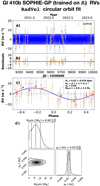 |
Fig. 9 Results of the RadVel model of one planet in circular orbit for the SOPHIE RVs corrected for activity using a GP that used SPIRou’s Bℓ measurements as an activity proxy. We note that only the 2021–2023 data was used, as these data have quasi-simultaneous SPIRou Bℓ data. The planet parameters obtained from the SOPHIE–GP RVs are very similar to those retrieved from the wPCA and Wapiti SPIRou data. |
RadVel model comparison table of the one-planet model of the combined SPIRou wPCA and SOPHIE–GP (trained on Bℓ) data sets.
7 Search for additional signals within the SPIRou wPCA data
As presented in Sect. 4.2 the GLS periodogram of the wPCA SPIRou RVs shows in addition to the 6.02 day peak a second peak at 18.76 days with FAPboostrap = 1.6%. The presence of additional planetary signals in the data is encouraging as it is known from transit searches that M-dwarfs often exhibit multi-planetary systems. In this section we investigate the possibility of having additional planetary signals within the wPCA SPIRou RVs.
7.1 Possibility of a planet at P = 18.7 days
If the 6.02-day Keplerian signal of Gl 410b (Table 9) is subtracted from the wPCA SPIRou time series and a new GLS periodogram is calculated on the residuals, we find that the signal at P = 18.76 days is still present. Furthermore, its FAPboostrap level improves to 0.3% (Fig. 10, middle panel). This provides tentative evidence in favor for the presence of a second planet.
To further test the plausibility of the existence of the signal at 18.7 days, we calculated a RadVel MCMC run using a two-planet model. For this test, we set broad uniform priors for Pb (0–20 days), Pc (0–30 days), and Kb and Kc (0 and 20 m s–1). Circular and eccentric orbit (e < 1) models were calculated. The model priors and initial guesses are summarized in Table E.1 in the Appendix. Our goal was to determine which planet solution is favored by RadVel and to compare the periods blindly retrieved by RadVel with those of the periodogram analysis.
The RadVel AICc model comparison is presented in Table E.2 in the Appendix. RadVel finds the two-planet solution more likely compared to one-planet solution. In fact, the models with one planet were “ruled out” by RadVel. RadVel favors a model in which planet b has an eccentric orbit and planet c has a circular orbit and a model in which both b and c have circular orbits. However, the two models are “nearly indistinguishable” for RadVel. We favor the model in which the two planets are in circular orbits.
In the Appendix, we provide the corner plots of the model with two planets in circular orbit (Fig E.1), a plot showing the phase-folded RVs, and the best fitting two-planet circular solution (Fig E.2). We also show a table summarising the retrieved orbital parameters and physical properties (Table E).
RadVel indicates for the candidate signal at 18.7 days a Mc sin(i) = 9.9 ± 1.8 M⊕ (Kc = 3.6 ± 0.7 m s–1) and a period Pc = 18.76 ± 0.03 days (ac = 0.113 ± 0.001 au). This period, retrieved blindly by RadVel, corresponds to the peak in the peri-odogram once the RV signal of Gl 410b is removed from the data (middle panel of Fig. 10). The properties of Gl 410b are similar to those retrieved in the one-planet model. We note that Mb sin(i) slightly decreases to 7.9 ± 1.2 M⊕, which is within the 1σ error of the one-planet model value. The bottom panel of Fig. 10 displays the periodogram of the residuals of SPIRou wPCA RVs after subtraction of the signal of Gl 410b and the candidate signal at 18.7 days. No peaks with a significance higher than FAP = 10% are left in the periodogram. We also tested a RadVel model on the combined SPIRou wPCA and SOPHIE–GP data set (not shown). In this data set, the model with two planets in circular orbit was favored by the AICc tests as well.
Thus, Gl 410 has tantalising evidence for hosting two sub-Neptune planets in circular orbits close to a 3:1 resonance. For curiosity, using the RadVel posterior distributions of the eccentric orbit models, we explored the stability of such a system (Appendix F). We found that the system is safely stable for circular orbits and the nominal eccentricity values.
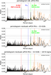 |
Fig. 10 Periodograms of the SPIRou wPCA data after subtraction of the circular orbit models of Gl 410b and the candidate planetary signal at 18.7 days. |
7.2 ℓ1 and apodized sine periodogram analysis
The results of the GLS periodogram and the two-planet RadVel modeling are promising. To perform an independent assessment on the existence of periodicities within the SPIRou wPCA data set, we performed a ℓ1 and apodized sine periodogram (ASP) analysis. The ℓ1 periodogram searches for several signals simultaneously, and the ASP tests the consistency in frequency, phase, and amplitude of the candidate signals. We used the ℓ1 periodogram technique as defined in Hara et al. (2017). This tool is based on a sparse recovery technique called the basis pursuit algorithm (Chen et al. 1998). It aims to find a representation of the RV time series as a sum of a small number of sinusoids whose frequencies are in the input grid. It outputs a figure that has a similar aspect as a regular periodogram but with fewer peaks due to aliasing. The peaks can be assigned an FAP, whose interpretation is close to the FAP of a regular periodogram peak.
The ℓ1 periodogram takes several parameters as input, in particular, a list of vectors, or predictor, that are fitted linearly along with the search for periodic signals. For this linear base model, we chose several stellar activity indicators available within the SPIRou data: the longitudinal magnetic field (Bℓ) measurement, the LBL projection onto the second derivative of the spectrum (d2v), the LBL projection onto the third derivative of the spectrum (d3v), the LBL differential line width (dLW), and LBL the differential temperature measurement (dTEMP) with respect to a T = 4000 K template. The LBL activity indicators are calculated at the same time as the RVs (Artigau et al. 2022, 2024). We also added a periodic signal at the sidereal day to account for apparent systematics at this period. The ℓ1 periodogram also necessitates to assume a certain form of the noise model. Following the method of Hara et al. (2020), we tested a grid of noise models, and ranked them with cross-validation and Bayesian evidence, which we computed with the Laplace approximation. The detailed analysis is presented in Appendix G.1.
In Figure 11, we represent the ℓ1 periodogram of the noise model with the highest cross-validation score. We found clear evidence for the 6.02-day signal with an FAP of 7.4 × 10⁻⁹. The 18.7-day signal is also present with a 7.3 × 10⁻³ FAP. We note the presence of an additional 2.99-day signal with an FAP 3.8 × 10⁻⁴. Finally, we found a marginally significant signal at 1.3 days. The signals at 6, 18, and 3 days are consistently found by the computed ℓ1 periodograms, they present peaks in 100% of the top 20% of the models with highest cross-validation scores.
To further refine the analysis, we tested whether the candidate signals are strictly periodic or if their frequency, phase, and amplitudes show signs of variation. For this, we employed the method of Hara et al. (2022), which consists in fitting apodized sinusoidal signals to the data set. These signals are wavelet-like, composed of a sine multiplied by a Gaussian function localized in time. In Appendix G.1, we show that there is good evidence that the three signals found by the ℓ1 periodogram are strictly periodic.
In summary, apart from the clear 6.02-day planet, we find in the ℓ1 and ASP analysis statistically significant candidates at 18.7 and 2.99 d, which are compatible with purely periodic signals. We note that the proximity of the 2.99 d planet to a 2:1 mean motion resonance with the 6-day planet further supports that it is indeed is a planet. This third planet would have a mass of a few Earth masses. Nonetheless, we do not label the two signals as confirmed planets, as their statistical significance is not completely sufficient.
To conclude this section, we insist that although the detections of the signals at 18.7 and 2.99 days pass several statistical tests, at the present they are candidate signals because they are only retrieved in the wPCA SPIRou data. Further measurements and improvements on the methods to recover the data in the |Vtot|<10 km s–1 region are required to fully exploit all the measurements taken and to ultimately confirm or refute the planetary nature of these signals.
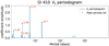 |
Fig. 11 ℓ1 periodogram of the model corresponding to the highest value of Bayesian evidence, calculated with the Laplace approximation. |
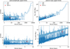 |
Fig. 12 Detection limits in the SPIRou wPCA RV time series. The left panels show the upper limits on the semi-amplitude K in meters per second. The right panels display the limits in terms of the projected mass m sin(i). A zoom-in of the period range from 1 to 10 days is presented in the lower panels. Objects with a projected mass above the light blue and dark blue lines are ruled out with a confidence level of 99% and 75%, respectively. The red dot indicates the location of Gl 410b. |
7.3 Planet detection limits at long periods from the SPIRou wPCA radial velocities
We computed the planet detection limits from the SPIRou RVs by performing an injection recovery test. The method determines the upper limits by injecting signals in the time series at given periods, calculating the GLS periodograms, and determining the maximum amplitude that can still be missed with a given probability. For each period, the upper limit is given by the highest amplitude (at the worst phase) that could be present in the time series without creating a peak above the 1% FAP level in the periodogram. The method consists of injecting for each period a sinusoidal Keplerian signal (i.e., circular orbit) at 12 equi-spaced phases. The amplitude (i.e., the planet signal strength) is then increased until the corresponding peak in the GLS periodogram reaches the 1% FAP level. The 1% FAP confidence level was computed from the levels of the highest peaks of 1000 permuted data sets, and the 1% upper limits was obtained by sorting the power of the peaks of all periodograms at each period. We tested periods from 0.8 to 10000 days.
Figure 12 displays the projected mass as a function of the period at which 99% and 75% of the planets injected would be detected in the GLS periodogram of the SPIRou data. The degraded upper limits for the periods around 1, 2, 180, and 360 days are due to the data sampling and are an unavoidable consequence of observing at night from a single location and from the fact that SPIRou is only mounted in bright time. Our SPIRou RV data can detect with a 99% confidence planets with masses larger than 0.1, 1.0 and 4.7 MJ at a periods of 100, 2560 and 5000 days (0.35, 3 and 5 au), respectively.
Kervella et al. (2022) performed a study aimed at detecting companions of Hipparcos catalog stars based on the proper motion anomaly derived from Hipparcos and Gaia measurements. Gl 410 is part of that study, and it displays a proper motion anomaly S/N of 0.13. Kervella et al. (2022) derived a companion mass of 0.02 MJ (6.3 M⊕) in a 3–5 au orbit. The mass of this companion candidate is significantly below the sensitivity capability of our current SPIRou RV measurements.
8 TESS photometry analysis
The TESS photometry time series is shown in Fig. 13. One can clearly observe the modulation of the TESS light-curve by the stellar rotation. However, it is not possible to measure the rotation period with high accuracy because the time span of the observations (~27 days) does not fully cover two complete rotation periods. No transits were identified by the TESS automatic pipeline. To further search for transit events, we applied a procedure customized for Gl 410. After removing the outliers using a 3σ clipping procedure, we used the package Wotan (Hippke et al. 2019) to flatten the light curve and to remove the effects of variability due to stellar rotation. The second panel of Fig. 13 displays the resultant detrended light curve, which has a scatter of 403 ppm. Using the transit least squares algorithm of Hippke & Heller (2019), we searched for periodic transit events in the detrended light-curve, in particular at the orbital period of planet b. The algorithm retrieved periodic signals at 3.5 and 7 days with a signal detection efficiency (SDE) on the order of 5, which is not high enough to claim a detection (Fig. 14). Further inspection of those signals revealed thay they are artifacts. The signals are close to the harmonics of the stellar rotation period and are likely related to residuals of the detrending procedure. No signal was detected at period of 6.02 days, suggesting that Gl 410b is not transiting.
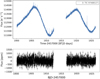 |
Fig. 13 TESS photometry data for Gl 410. Upper panel: presearch Data Conditioning flux time series processed by the TESS Science Processing Operations Center. Second panel: Wotan (Hippke et al. 2019) detrended light curve. |
8.1 Transit detection limits
To determine the detection limits in the TESS data, we conducted an injection recovery test of transit events. Following Cortés-Zuleta et al. (2025), using the stellar parameters of Gl 410 and the semimajor axis of 0.053 au, we injected 50 000 transits generated with the software batman (Kreidberg 2015), for which the orbital inclination and planet radius are drawn randomly from uniform distributions: between 85° and 90° for the inclination and from 0.1 to 10 R⊕ for the radius. For each synthetic transit, we computed the box least squares periodogram11 implemented in astropy and measured the power of the signal at a period of 6.02 days. Then, we measured the fraction of transit events that are detectable with the box least squares periodogram (i.e., power > 1000). The results of the injection test are shown in Fig. 15. We fond that planets with a radius smaller than 1.8 R⊕ are not detectable in the current TESS data as well as planets in orbits with inclinations lower than 87 deg.
9 Discussion
9.1 Gl 410b in context
Gl 410b sums up to the growing list of sub-Neptune mass planets detected around low-mass stars (M < 0.6 M⊙). In order to place the Gl 410 planetary system in context, in this section we concentrate on discussing the planet detection statistics of the stars in the 0.5–0.6 M⊙ stellar mass bin, that is, the stars with a mass equal to that of Gl 410. At the time of writing (1 July 2024), this stellar mass range, according to the NASA exoplanets catalog12, has 212 planet candidates detected (of 5678 exoplanets). Several of those planets are awaiting further characterization, but 140 already have a reported radius measurement, 83 have a planetary mass measurement and, 30 have a mass constraint (i.e., Mb sin(i)).
The period is always determined in transit and in RV planet detections. However, in both methods, detection statistics are strongly positively biased to short periods, as planets in short periods are the easiest to detect. At the time of writing, in the 0.5–0.6 M⊙ stellar mass bin, of the 212 planet candidates, there are 161 detections at Porbit < 50 days, with 80% of those detections at Porbit < 15 days. These numbers illustrate the observational biases mentioned. Perfoming a detailed study correcting for biases is out of the scope of this discovery paper; however, we can point out that planets in a 6-day period, such as Gl 410b, are not unusual in the 0.5–0.6 M⊙ stellar mass bin.
Concerning the planet mass, we are interested in discussing how abundant or scarce planets are in the mass range of Gl 410b (8.4 ± 1.3 M⊕) in orbits with periods Porbit < 50 days around stars in the 0.5–0.6 M⊙ stellar mass bin. We show in Fig. 16 the histograms of the planet mass distribution for a Porbit < 10 days (top panel) and for Porbit between 10 and 50 days (bottom panel). The histogram includes both mass measurements and Mb sin(i) lower limits. In the subsample with Porbit < 10 days, the most abundant planets are those with masses less than 10 M⊕, with ~40% of the detections. These are followed by planets with mass between 1/3 and 1 MJ, with 23% of the detections. Detection biases make planets with masses less than 10 M⊕ the hardest to detect. The large fraction of detections of planets in the low mass range means that they should intrinsically be the most numerous. The histograms show a significant decrease on the frequency of planets for the mass bin between 17 Μ⊕ (Neptune mass) and 100 Μ⊕ (~l/3 MJ). As planets in this mass range are more easily detected by RVs than planets with Μ < 10 Μ⊕, the decrease is real, and it is not a detection bias. We find that Gl 410b is located in the bin with the highest probability of detection.
In the context of the subsample of planets with periods between 10 and 50 days, we find that (i) the mass bin between 5 and 10 Μ⊕ has the highest fraction of detections, (ii) there is a decrease in the number of detections of planets with M < 5 Μ⊕, and (iii) there are very few detections of giant planets. The smaller fraction of low-mass planets could be an observational bias given the fact that detecting planets with M < 5 Μ⊕ around M dwarfs at longer periods is likely harder because the amplitude becomes smaller, and it could be comparable to the activity jitter. The very small fraction of giant planets, in contrast, is not an observational bias, and it must be real, as giant planets are easier to detect through RVs. The tentative planet candidate signal at 18.7 days would thus belong to the category of the most frequently detected planets.
The very fact that Gl 410b is located in the bins with the highest number of detections reinforces the current view that sub-Neptune mass planets are abundant around M dwarfs. The decrease of the occurrence rate with increasing planetary mass is a property that has already been highlighted in studies covering the entire M dwarf mass domain (e.g., Bonfils et al. 2013; Sabotta et al. 2021; Mignon et al. 2025). Current statistics raise the question of why planets with masses between Neptune and 1/3 MJ are scarce at periods shorter than 50 days around stars whose mass is in the 0.5–0.6 M⊙ mass bin. Whether this could be a consequence of the planet formation process, or a product of the interaction of planetary atmospheres with energetic radiation and stellar wind particles due to the high activity levels of M dwarfs is an open question.
Since Gl 410b is not transiting, we do not have a stringent constraint on its radius. Based on the sample of planets in the 0.5–0.6 M⊙ stellar mass bin with Porbit < 50 days and masses similar to Gl 410b (7–10 M⊙), at present there are only a few planets for whom measurements of the radius are available, for example, TOI-1725b (Rp = 1.8 ± 0.1 R⊕, Mp = 9.9±1.3 Μ⊕, Essack et al. 2023) and TOI-2018b (Rp = 2.27 ± 0.07 R⊕, Mp = 9.2±2.1 Μ⊕, Dai et al. 2023).
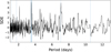 |
Fig. 14 Wotan signal detection efficiency as a function of the period. The vertical light blue line at 3.5 days is the period with the highest SDE, and the dashed lines correspond to its harmonics. We note that the signal is not significant. |
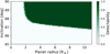 |
Fig. 15 Results of the injection recovery test in the TESS data. The figure shows the probability of detection of a transit for a given planet radius and orbit inclination. |
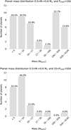 |
Fig. 16 Histograms of planet detections in the 0.5–0.6 M⊙ stellar mass bin. Data from the NASA exoplanets catalog as of 1 July 2024. |
9.2 Stellar activity and the evolution of Gl 410b
Let us conclude this section by briefly discussing the implications of stellar activity in the atmospheric evolution of Gl 410b13. As presented in Section 2, Gl 410 is an active star. Activity is the manifestation of the presence of stellar magnetic fields. Magnetic fields heat the chromosphere and coronae and drive stellar winds (e.g., Cranmer & Winebarger 2019). High-energy radiation from stellar flares and X-ray/EUV coronal emissions and particle fluxes from winds and coronal mass ejections interact with the magnetospheres and the atmospheres of planets in orbits close to the star, thus driving thermal and non-thermal atmospheric escape processes (for recent reviews see Vidotto 2022; Kubyshkina 2024).
As Gl 410b is located very close to its host star at 0.05 au, it is therefore expected to have an active interaction with the high-energy radiation and the stellar wind particle fluxes from Gl 410. Using the radius and Teff given in Table 1, we obtained that Gl 410b receives 20.4 × Earth’s insulation. It is out of the scope of this discovery paper to perform a detailed study on the conditions on which a planet with 9 Earth masses could retain its atmospheres in the case that it is in the proximity of an active M dwarf such as Gl 410, but it is an interesting topic that deserves further study. Furthermore, it would be of extreme interest to investigate the influence that stellar irradiation and activity could have in the chemical composition of the planet’s atmosphere and the potential development of abundance anomalies due to the escape of volatile species (e.g., Louca et al. 2023) in single- and multi-planetary systems (e.g., Acuña et al. 2022).
10 Conclusion
In this paper, we have presented an RV study of Gl 410, a nearby (d = 12 pc) early M dwarf with a mass of 0.55 M⊙ and an age of 480 ± 150 Myr14. We monitored the star in the near-IR with the spectropolarimeter and velocimeter SPIRou and in the optical with the velocimeter SOPHIE. The SPIRou RVs show a robust periodic signal at P = 6.020 ± 0.004 days. The signal is recovered in the raw LBL data and in the two PCA methods used to correct the LBL RVs for systematics and telluric correction residuals. In our baseline solution, the circular orbit model of the SPIRou wPCA data set (Table 9), the signal has a semi-amplitude of 4.4 ± 0.7 m s–1, which indicates a sub-Neptune planet with M sin(i) of 8.4 ± 1.3 Earth masses at 0.0531 ± 0.0006 au. The same Keplerian signal is recovered in quasi-simultaneous SOPHIE RV measurements after correction for stellar activity using a GP that was trained on the measurements of the longitudinal magnetic field (Bℓ) obtained with SPIRou. The independent detection of Gl 410b in the SOPHIE RVs provides further evidence for the Keplerian nature of the periodic signal.
We searched the TESS archive and investigated whether Gl 410b could be a transiting planet. We found no evidence for the transit of Gl 410b. A recovery analysis on the TESS photometry indicates that the transit would have been detected if Gl 410b’s inclination were higher than 87 deg and its radius were larger than 1.8 R⊕. Gl 410b is located very close to its host star, and it receives 20.4 times Earth’s insulation. It would be of great interest to investigate the influence that stellar irradiation and activity could have on the chemical composition of the planet’s atmosphere and in the potential atmospheric escape processes.
We find within the SPIRou wPCA RVs, there is tentative evidence for two additional planetary signals at 2.99 and 18.7 days. The 18.7-day signal (which is consistent with a sub-Neptune planet) is directly seen in the GLS periodograms and it is recovered in a RadVel two-planet model with broad priors for the period. The 2.99-day signal emerges together with the 18.7-day signal in an ℓ1 and apodize sine periodogram analysis, which takes into account stellar activity indicators measured with SPIRou and a model for the correlated noise. The planet at 2.99 days could be in a 2:1 mean motion resonance with the 6.02-day planet and could have a mass of a few Earth masses.
The detection of Gl 410b shows that infrared RVs are a powerful tool for detecting planets around active stars, objects which are often excluded from searches in optical RVs. Care should be taken, however, to correct and filter systematics generated by residuals of the telluric correction or small structures in the detector plane. The LBL technique combined with PCA offers a promising way to reach this objective. This approach enabled us to use the RV measurements acquired when the star is at ±10 km s–1 of the center of the telluric absorption lines, which is important to detect additional planetary signals. Further monitoring of Gl 410 is necessary.
Data availability
Full Tables 2, 3, 5 are available at the CDS via https://cdsarc.cds.unistra.fr/viz-bin/cat/J/A+A/700/A222.
Acknowledgements
Based on observations obtained at the Canada-France-Hawaii Telescope (CFHT) which is operated from the summit of Maunakea by the National Research Council of Canada, the Institut National des Sciences de l’Univers of the Centre National de la Recherche Scientifique of France, and the University of Hawaii. Based on observations obtained with SPIRou, an international project led by Institut de Recherche en Astrophysique et Planétologie, Toulouse, France. Based on observations obtained with the spectrograph SOPHIE at the Observatoire de Haute-Provence (OHP) in France, operated by Institut National des Sciences de l’Univers of the Centre National de la Recherche Scientifique of France. We acknowledge funding from the French ANR under contract number ANR18CE310019 (SPlaSH). This work is supported by the French National Research Agency in the framework of the Investissements d’Avenir program (ANR-15-IDEX-02), through the funding of the “Origin of Life” project of the Grenoble-Alpes University. JFD acknowledges funding from the European Research Council (ERC) under the H2020 research & innovation program (grant agreement #740651 NewWorlds). This publication makes use of the Data & Analysis Center for Exo-planets (DACE), which is a facility based at the University of Geneva (CH) dedicated to extrasolar planets data visualization, exchange and analysis. DACE is a platform of the Swiss National Centre of Competence in Research (NCCR) PlanetS, federating the Swiss expertise in Exo-planet research. The DACE platform is available at https://dace.unige.ch. The project leading to this publication has received funding from the french government under the “France 2030” investment plan managed by the French National Research Agency (reference: ANR-16-CONV-000X / ANR-17-EURE-00XX) and from Excellence Initiative of Aix-Marseille University – A*MIDEX (reference AMX-21-IET-018). This work was supported by the “Programme National de Planétologie” (PNP) of CNRS/INSU. E.M. acknowledges funding from FAPEMIG under project number APQ-02493-22 and research productivity grant number 309829/2022-4 awarded by the CNPq, Brazil. This work has made use of data from the European Space Agency (ESA) mission Gaia (https://www.cosmos.esa.int/gaia), processed by the Gaia Data Processing and Analysis Consortium (DPAC, https://www.cosmos.esa.int/web/gaia/dpac/consortium). Funding for the DPAC has been provided by national institutions, in particular the institutions participating in the Gaia Multilateral Agreement. The observations at the Canada-France-Hawaii Telescope were performed with care and respect from the summit of Maunakea which is a significant cultural and historic site.
Appendix A On the age of Gl 410
Age determination using gyrochronology rely on empirical relations between the rotation period and the effective temperature or photometry of stars in clusters of known ages. The age of 0.89 ± 0.1 Gyr for Gl 410 derived in Fouqué et al. (2023) was determined using the methods described in Gaidos et al. (2023) which are calibrated on the empirical relations of Curtis et al. (2020). In Fig. A.1, we display the Prot vs Teff diagram from Curtis et al. (2020), indicating the location of Gl 410 in solid lines. At the Teff Gl 410, the age-rotation relations of Praesepe (670 Myr) and NGC 6811 (1 Gyr) sequences overlap. The rotational period of Gl 410 locates the star below the Praesepe sequence, which suggests that Gl 410 could be younger than 670 Myr. The Gaidos et al. (2023) work targeted the vast majority of planet hosts which are middle-aged and did not use calibrations below the Praesepe age so by definition no claim for a younger age could be done.
To investigate the possibility of a younger age for Gl 410, we estimated its age using two alternative publicly available gyrochronology codes: stardate (Angus et al. 2019) and gyro-inter (Bouma et al. 2023). Both codes converge in a younger age estimate for Gl 410: stardate suggests an age of 493 ± 2 Myr; gyro-inter indicates an age of  Myr. Furthermore, we checked the position of Gl 410 in the color-magnitude diagram (CMD). The right panel of Fig. A.1 displays the Gaia DR3 (Gaia Collaboration 2023) CMD for Gl 410, field stars, together with empirical CMD sequences from various young associations (Gagné et al. 2021). Gl 410 is located between the 400 and 580 Myr sequences. Interpolating in log space, an age of about 480 Myr is obtained for Gl 410. We note, however, that the scatter around these empirical sequences is non negligible, that at younger ages the age distribution is complex and likely non Gaussian, and that the age is anchored on the ages assumed for Group X (Oh et al. 2017) and Coma Ber. From the empirical sequences, we find that Gl 410 is slightly younger than Praesepe that is somewhat unlikely to be as young as the Pleiades (~120 Myr, although the probability is not 0%), and very unlikely to be as young as the Tucana-Horologium association (~45 Myr). Based on these considerations, we propose an age of 480 ± 150 Myr for Gl 410. Further dedicated work is necessary to determine the age of Gl 410 with a higher precision, but this study is beyond the scope of this paper. A possible way to narrow-down the uncertainty, would be to map the distribution of reference age populations at this spectral type, reverse the distribution using Bayes theorem and Gl 410’s rotational period and then obtain a non-gaussian age probability distribution for Gl 410.
A young age for Gl 410 is of interest because it suggest that Gl 410 might be related to the Ursa Major (UMA) cluster which is approximately 400 Myr old. Gl 410 indeed has been previously suggested to be member of UMA by Ammler-von Eiff & Guenther (2009), member of a diffuse region associated with UMA by King et al. (2003) and member of the “UMA moving group” by Montes et al. (2001). The Galactic UVW velocities of Gl 410 appear consistent with the proposed Ursa Major corona (Gagné et al. 2020).
 |
Fig. A.1 Left panel: Rotational period vs effective temperature for stars in clusters of different ages from Curtis et al. (2020). The location of Gl 410 is indicated in solid lines (error on Teff is given in light red). Right panel: Gaia DR3 color-magnitude diagram of young stars with calibrated ages (dots) and empirical age sequences from young associations (Gagné et al. 2021). The position of Gl 410 is indicated with a red dot. Gl 410 is located between the 400 and 580 Myr sequences. |
Appendix B Activity analysis
We measured activity indicators in the SOPHIE and SPIRou spectra. For the SOPHIE data set, the activity indicators were derived based on distortions of the cross-correlation function (CCF), the bisector (BIS), the full width half maximum (FWHM), and the CCF contrast, and on the spectral line indexes Hα and S index (based on the Ca II H&K lines, calculated as described by Boisse et al. 2009). We investigated the temporal evolution of the activity indicators calculating GLS periodograms and searching for modulations related to the stellar rotation. The periodograms of the SOPHIE activity indicators are shown in Fig. B.1 and B.2. Considering the whole ensemble of SOPHIE activity indicators, none of their periodograms display a peak at the stellar rotation period (13.91 days), with exception of Hα and the S index that show excess power below 0.1% FAP around 15 and 16 days, periods which are relatively close to the stellar rotation period. To check for consistency, we also computed GLS periodograms for the SOPHIE data set split in two periods: 2010–2012 and 2021–2023. The periodograms of the 2010–2012 period do not display significant periodicities except for Hα which exhibits several peaks at periods between 14 and 19 days, however, they are most likely be due to poor sampling. In the case of the 2021–2023 period, the periodogram of the S index exhibits a significant periodicity (<1% FAP) at 15.3 days and more importantly, the BIS shows excess power almost at 1% FAP at 14 days, which is consistent with the rotation period.
For the SPIRou data set, we analyzed the GLS periodograms of the differential line width (dLW), the FWHM, and the chromatic velocity slope calculated by the LBL algorithm. The periodograms are shown in Fig. B.3. We found excess power at ~13 days in the dLW and chromatic velocity slope periodograms. This periodic variability could be related to the stellar rotation. No periodicities are detected at 6.02, 18.7 nor 2.99 days neither in the SOPHIE nor SPIRou data sets.
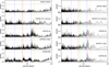 |
Fig. B.1 Periodograms of the SOPHIE activity indicators: FWHM, CCF contrast, Hα, S index, and BIS. The left periodograms correspond to the whole data set, the right periodograms correspond to the 2010–2012 period. The vertical dashed lines depict: in red, 6.02 days; in blue, the rotation period with its harmonic in green; in orange, 18.7 days, and, in purple dots, 2.99 days. The horizontal dashed lines indicate the 1% and 0.1% FAP levels. |
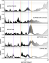 |
Fig. B.2 Periodograms of the SOPHIE activity indicators: FWHM, CCF contrast, Hα, S index, and BIS for the 2021–2023 period. The vertical dashed lines depict: in red, 6.02 days; in blue, the rotation period with its harmonic in green; in orange, 18.7 days, and, in purple dots, 2.99 days. The horizontal dashed lines indicate the 1% and 0.1% FAP levels. |
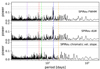 |
Fig. B.3 Periodograms of the SPIRou activity indicators: FWHM, dLW, and chromatic velocity slope. The vertical dashed lines depict: in red, 6.02 days; in blue, the rotation period with its harmonic in green; in orange, the 18.7 days, and, in purple dots, 2.99 days. The horizontal dashed lines indicate the 1% and 0.1% FAP levels. |
Appendix C Gaussian process modeling of SPIRou’s longitudinal magnetic field
Measurements of the longitudinal magnetic field (Bℓ) of Gl 410 taken with SPIRou have been previously presented and analyzed in Fouqué et al. (2023) and Donati et al. (2023). Fig. C.1 displays the LS periodogram of the Bℓ data from Donati et al. (2023). We retrieve the peak at Ρ = 13.87 days which is associated with to 13.91 ± 0.09 day rotational period of the star and its lyr alias at 14.98 days. One additional peak with FAP level below 0.1%, and not related to the window function, is detected at 9.41 days with its lyr alias at 9.69 days. No peak is observed at 6 days. Using the python module george (Foreman-Mackey 2015), we fitted a GP on the SPIRou Bℓ time series using a quasi-periodic kernel of the form:
 (C.1)
(C.1)
where A is the amplitude, Γ is the smoothing parameter, l is the decay time in days, Ρ is the period (i.e., the cycle length) in days, and σ is the uncorrelated noise (s in the corner plots). We used uniform distributions for the priors of the amplitude, decay time, smoothing, cycle length, and uncorrelated noise as described in Table C.1. The distribution of the hyperparameters was sampled using the Markov chain Monte Carlo (MCMC) implemented in the EMCEE tool (Foreman-Mackey et al. 2013). We used 100000 samples and 10000 burn-in samples. In Table C.1 and Fig. C.1, we summarize the results of the GP modeling of the Bℓ time series. Fig. D.1 present the corner plots of the fit. As expected, we retrieve in our Bℓ GP the stellar rotational period of 13.93 ± 0.09 days which is consistent with the previous determinations of the rotational period by Donati et al. (2023) and Fouqué et al. (2023). The values obtained for the amplitude, decay time and smoothing parameter are consistent to those of Donati et al. (2023).
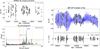 |
Fig. C.1 Left panel: SPIRou Bℓ measurements from Donati et al. (2023) and associated LS periodogram. The horizontal dashed lines represent the FAP levels of 0.1%, 1%, and 10% respectively. A significant peak at Ρ = 13.87 days (and lyr alias at 14.98 days) is clearly observed, which is associated with to 13.91 ± 0.09 day rotational period of the star Donati et al. (2023). An additional significant peak is seen at 9.41 days. No signals are seen at Ρ = 6.02 days. Right panel: quasi-periodic GP model fit (blue-line) of the SPIRou Bℓ time series (black dots). Details of the GP are given in Table C.1. The corner plot of the fit is given in Fig. D.1. |
Prior and posterior distributions of the quasi-periodic GP models fit to the SOPHIE RV time series and the SPIRou Bℓ measurements.
Appendix D Corner plots and additional figures and tables of the one-planet model
 |
Fig. D.1 Corner plot of the quasi-periodic GP fit of the SPIRou longitudinal magnetic field (Bℓ) time series of Gl 410. We provide the description of the meaning of the variables in Table C.1. |
 |
Fig. D.2 Corner plot of the quasi-periodic GP fit of the SOPHIE RVs using the posterior distributions of the decay time, smoothing length and γ of the GP on the SPIRou Bℓ time series as priors. We provide the description of the meaning of the variables in Table C.1. |
 |
Fig. D.3 Corner plots of the posterior distributions of the RadVel MCMC one-planet circular orbital model of the SPIRou RV time series selecting the measurements at |Vtot| > 10 km s–1. |
 |
Fig. D.4 Corner plots of the posterior distributions of the RadVel MCMC one-planet circular orbital model of the SPIRou wPCA RV time series |
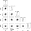 |
Fig. D.5 Corner plots of the posterior distributions of the RadVel MCMC one-planet circular orbital model of the SPIRou Wapiti RV time series. |
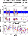 |
Fig. D.6 Best-fitting one-planet RadVel circular orbit model for the data set combining the SPIRou wPCA RVs and the SOPHIE RVs corrected for activity using Bℓ as an activity proxy. The T perib retrieved is 59646.6 ± 0.15. The uncorrelated noise of the fit are σSPIRou = 5.6 ± 0.4 m s–1 and |

Appendix Ε Corner plots and additional figures and tables of the RadVel two-planet model
Priors and initial guess values of the RadVel two-planet model run on the SPIRou wPCA RV time series.
RadVel model comparison table of the one and two-planet models for the SPIRou wPCA data set.
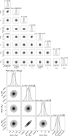 |
Fig. E.1 Corner plots of the posterior distributions of the RadVel MCMC two-planet circular orbital model of the SPIRou wPCA RV time series. |
Orbital parameters and planet physical properties derived from a RadVel MCMC two-planet in circular orbit model of the SPIRou wPCA data.
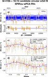 |
Fig. E.2 RadVel best fitting two-planet in circular orbits model derived from the wPCA SPIRou RVs. |
Appendix F Dynamical stability analysis
While somehow limited constraints on the orbital configuration can be obtained from the RV measurements, we performed a dynamical stability assessment for the two-planet system Gl 410b and 18.7-day candidate to consolidate the picture on the system architecture. The period ratio (larger than 3) is wide and Gl 410 b and the 18.7-day candidate are small enough that the system is safely stable for circular orbits and the nominal eccentricity values. Indeed the orbital separation in Hill radii is of ac – ab = 23 ± 1.5 RH which is far beyond the stability limit of 3.46 RH (Gladman 1993). Although we favor a model with circular orbits, we can derive some constraints on the maximum stable eccentricities by computing the general Hill stability criterion as described in Petit et al. (2018). We take the RadVel posterior and compute the Angular Momentum Deficit (AMD) of the system as well as the critical value ensuring Hill stability (in other words, the maximum AMD such that close encounters are always forbidden). In Fig. F.1, we compare the posterior eccentricity distribution resulting from the RadVel RV fit and the posterior eccentricity distribution only keeping the stable configurations. Rejecting Hill unstable configurations from the posterior, we obtain an upper limit for ec at 0.4 but no additional constraints on eb. Stable configurations are on average more circular. A similar analysis on the masses show that no stringer constraints can be drawn from the stability on this system.
The Hill stability can also constrain the maximum mutual inclination. To obtain this constraint, we assume that the system invariant plan is aligned with the line of sight15 and we assign a random mutual inclination to each configuration in the posterior. Computing the critical AMD in this case, we find that systems with a mutual inclination smaller than 40 degrees are stable. As for the eccentricities, this is mainly an upper limit. The system is fully consistent with coplanar orbits.
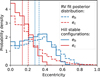 |
Fig. F.1 Eccentricity distributions of Gl 410b and the 18.7-day candidate signal with the distributions for Hill stable configurations. The vertical lines indicate the mean of the respective distributions. |
Appendix G Additional radial velocity analysis of the SPIRou wPCA data
G.1 ℓ1 periodogram analysis
The ℓ1 periodogram has several inputs: the RV time series to be analyzed, its nominal uncertainties, a grid of frequencies ω, a linear model assumed to be in the data M0, an assumed covariance matrix V of the noise as input. Overall, the model of the RV time series y(t) can be described by the equation
 (G.1)
(G.1)
where ϵ is a Gaussian noise with a certain covariance. Overall, the free parameters of the models are the coefficients of the linear model, x, the coefficients of periodic signals Ak, Bk, and the covariance parameters, which describe the properties of the noise. In practice, one chooses a parametrization of the covariance matrix of the noise V(θ), where the element of V at index k, l depends on |tk – t| and a vector of parameters θ. In the following analysis, the parametrization chosen for V is such that its element at index k, l is
 (G.2)
(G.2)
where σk is the nominal measurement uncertainty, σW is an additional white noise, σC is a calibration noise, and where c equals one if measurements k and l are taken within the same night and zero otherwise. The quantities σR and τR parametrize a correlated noise, which might originate from the star or the instrument. Additionally, σQP, τQP, and Pact parametrize a quasi-periodic covariance, potentially resulting from spots or faculae.
The ℓ1 periodogram looks for a small number of frequencies such that the model in Eq. (G.1) approximates the data. Depending on the different assumptions on the noise model and base linear model, the ℓ1 periodogram might find signals at different frequencies. To test the robustness of the results to a change in the model, we adopt the methodology of Hara et al. (2020). We consider a grid of potential noise models. For each of them, we computed the ℓ1 periodogram, and kept the signals that have a false alarm probability below 0.1. For each noise model in the grid, we then have candidate periodic signals. To each couple noise model/periodic signals, we attribute a cross-validation score. The model is fitted on 60% of the data points (the training set), and the likelihood of its prediction on the remaining 40% (the test set) is computed. This operation is repeated for 300 random draws of selection of training sets, and the final cross-validation score is computed as the average of the likelihood of the test set. We also rank the model according to their Bayesian evidence, evaluated with the Laplace approximation (see Hara et al. 2020; Nelson et al. 2020).
In our analysis, we adopt as M0 an eight-column matrix. Its columns are: an offset, the spectral shape indicators (i.e., stellar activity proxies): the SPIRou longitudinal magnetic field (Bℓ), and the LBL-derived (Artigau et al. 2022, 2024) projection onto the 2nd derivative of the spectrum (d2v), projection onto the 3rd derivative of the spectrum (d3v), differential line width (dLW), and differential temperature with respect to a T = 4000 K template (dTEMP4000) and, finally, a cosine and sine term at the sidereal day (period equal to 0.997 days). The grid of values chosen for the noise model is given in Table G.3. All the possible combinations of the values of its components were generated, and the corresponding covariance matrices were created according to Eq. (G.2). In G.1, we represent the histogram of cross-validation scores.
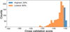 |
Fig. G.1 Histogram of the cross-validation score of the tested models. The blue histogram represents the counts of the 20% highest models. |
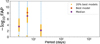 |
Fig. G.2 False alarm probability (FAP) of the signals appearing in the 20% of models with the highest Bayesian evidence (Laplace approximation). Each yellow point represents the FAP of a signal included in the model. Purple points represent the median values of the FAPS, and the red ones indicate the FAP of the highest ranked model. |
The ℓ1 periodogram corresponding to the highest ranked model is represented in Fig. 11. It shows four clear peaks at 6, 3, 18 and 1.3 days. To evaluate the robustness of these detections to the noise model, for each the 20% highest ranked models, we report the false alarm probabilities of the peaks found. The false alarms of the highest ranking models are reported in Fig. G.2. The percentage of cases where the 6, 3, 18 and 1.3 days signals were found in the 20% best models, the FAPs corresponding to the highest ranked model, and the median FAPs are reported in Table G.1. We find that the 6, 3, 18 days signal are present in a 100% of the highest ranked models, with median false alarm, probabilities of 7.5 × 10⁻⁸, 1.5 × 10⁻⁴ and 5.6 × 10⁻². The highest ranked models by Bayesian evidence give a similar picture, although they seem to provide more statistical significance for the signals (see Table G.2). They can be considered respectively as a confirmed planet, a very strong candidate, and a strong candidate.
G.2 Apodized sine periodogram analysis
To further examine the properties of the signals, we apply the method of Hara et al. (2022), which aim at testing whether the signals have a consistent amplitude, phase and frequency over time, which are the properties expected for planetary signals. For this we compute apodized sine periodograms (ASPs), defined as follows.
Inclusion of periodicities in the ℓ1 periodogram
Inclusion of periodicities in the ℓ1 periodogram. The models are ranked by Bayesian evidence.
Value of the parameters used to define the grid of models tested.
We compared the χ2 of a linear base model H, and the χ2 of a model K(ω, t0, τ) defined as the linear model of H plus an apodized sinusoid  (A cos ωt + B sin ωt). The ASP is defined as the χ2 difference between the two models
 (G.3)
(G.3)
We used the same base model as in our analysis with the ℓ1 peri-odogram, and used the covariance that corresponds to the noise model with highest Bayesian evidence.
To compute the ASP, we consider a grid of timescales τ = 10 · Tobs, Tobs/3, Tobs/9 and Tobs/27, where Tobs is the total observation timespan of the data. In Fig. G.4.a, left panel, we represent z(ω, t0, τ) as defined in Eq. (G.3), maximized over t0 for the values of τ in the grid. In other words, we always select the center of the time window which best fits the data.
We searched iteratively for signals. Once the maximum peak of the ASP was found, we then included the corresponding model in the base linear model H, and repeated the process. The four first iterations are shown in Fig. G.4, a, b, c, and d respectively. The left panels represent the periodograms, the middle panels a zoom in on the highest peak, and the right hand panel represents a statistical significance test, explained below.
In Fig. G.4.a, the dominating peak has a period of 6.02 days. We want to test whether the signal is statistically compatible with a constant one (i.e., with τ = 10 · Tobs). Denoting by t(τ,ω) the value of t0 maximizing the value of the periodogram (G.3) for a given ω and τ, we compute the distribution of
 (G.4)
(G.4)
with the hypothesis that the model K(ω, t(τ,ω), τ, A★, B★) is correct, where the fitted cosine and sine amplitudes A★, B★ are obtained by fitting model K to the data. Dz can easily be expressed as a generalized χ2 distribution, with mean and variance is given by an analytical expression (Hara et al. 2022).
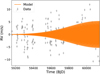 |
Fig. G.3 Best-fitting apodized sine model after three iterations. |
We find that even if the best fitting model for the 6.02 signal is not the purely periodic signal, it is still compatible with a purely periodic one. In Fig. G.3.b and c we see that the candidate signals at 2.99 and 18 days are compatible with strictly sinusoidal signals. In the case of the former, other signal shapes are excluded.
In the next iteration, in Fig. G.3.d, we find that the best fitting model is a short term signal at 5.78 days. In Fig. G.3, we show the corresponding model, which points to a transient signal. possibly caused by outliers or stellar variability.
Since the d3v vector, used in our linear base model M0, has shown in other SPIRou data set to be less reliable16 we re-did the whole analysis with the ℓ1 and ASP periodograms without it. The only notable difference is that it seems to slightly decrease the stability of the 18.7 day signal in frequency, amplitude and phase. We note that the 2.99 day planet could be in 2:1 mean motion resonance with the 6 d planet. In Hara et al. (2019), it has been shown that eccentric planets can mimic 2:1 mean motion resonances. However, it is very unlikely the case here, as the 2.99 d signal is significant and sharp. In conclusion, both 18.7 and 2.99 d planets are viable candidates, but the evidence for the latter is stronger.
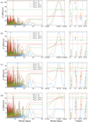 |
Fig. G.4 Four first iterations of the ASPs method. Models correspond to the maximum of the ASPs. The left panels represent the periodograms. the middle panels a zoom in on the highest peak, and the right hand panel represents a statistical significance test (see text for details). |
References
- Acuña, L., Lopez, T. A., Morel, T., et al. 2022, A&A, 660, A102 [NASA ADS] [CrossRef] [EDP Sciences] [Google Scholar]
- Ammler-von Eiff, M., & Guenther, E. W. 2009, A&A, 508, 677 [NASA ADS] [CrossRef] [EDP Sciences] [Google Scholar]
- Angus, R., Morton, T., & Foreman-Mackey, D. 2019, J. Open Source Softw., 4, 1469 [NASA ADS] [CrossRef] [Google Scholar]
- Artigau, É., Astudillo-Defru, N., Delfosse, X., et al. 2014, SPIE Conf. Ser., 9149, 914905 [NASA ADS] [Google Scholar]
- Artigau, É., Cadieux, C., Cook, N. J., et al. 2022, AJ, 164, 84 [NASA ADS] [CrossRef] [Google Scholar]
- Artigau, É., Cadieux, C., Cook, N. J., et al. 2024, AJ, 168, 252 [Google Scholar]
- Astudillo-Defru, N., Bonfils, X., Delfosse, X., et al. 2015, A&A, 575, A119 [NASA ADS] [CrossRef] [EDP Sciences] [Google Scholar]
- Bailer-Jones, C. A. L., Rybizki, J., Fouesneau, M., Demleitner, M., & Andrae, R. 2021, AJ, 161, 147 [Google Scholar]
- Bellotti, S. 2023, PhD thesis, IRAP, France [Google Scholar]
- Bellotti, S., Morin, J., Lehmann, L. T., et al. 2024, A&A, 686, A66 [NASA ADS] [CrossRef] [EDP Sciences] [Google Scholar]
- Bertaux, J. L., Lallement, R., Ferron, S., Boonne, C., & Bodichon, R. 2014, A&A, 564, A46 [NASA ADS] [CrossRef] [EDP Sciences] [Google Scholar]
- Boisse, I., Moutou, C., Vidal-Madjar, A., et al. 2009, A&A, 495, 959 [NASA ADS] [CrossRef] [EDP Sciences] [Google Scholar]
- Bonfils, X., Delfosse, X., Udry, S., et al. 2013, A&A, 549, A109 [NASA ADS] [CrossRef] [EDP Sciences] [Google Scholar]
- Bouchy, F., Hébrard, G., Udry, S., et al. 2009, A&A, 505, 853 [NASA ADS] [CrossRef] [EDP Sciences] [Google Scholar]
- Bouchy, F., Díaz, R. F., Hébrard, G., et al. 2013, A&A, 549, A49 [NASA ADS] [CrossRef] [EDP Sciences] [Google Scholar]
- Bouchy, F., Doyon, R., Artigau, É., et al. 2017, The Messenger, 169, 21 [NASA ADS] [Google Scholar]
- Bouma, L. G., Palumbo, E. K., & Hillenbrand, L. A. 2023, ApJ, 947, L3 [NASA ADS] [CrossRef] [Google Scholar]
- Cadieux, C., Doyon, R., Plotnykov, M., et al. 2022, AJ, 164, 96 [NASA ADS] [CrossRef] [Google Scholar]
- Carmona, A., Delfosse, X., Bellotti, S., et al. 2023, A&A, 674, A110 [NASA ADS] [CrossRef] [EDP Sciences] [Google Scholar]
- Chauvin, G. 2024, Comptes Rendus Phys., 24, 139 [Google Scholar]
- Chen, S. S., Donoho, D. L., & Saunders, M. A. 1998, SIAM J. Sci. Comput., 20, 33 [Google Scholar]
- Chen, X., Ge, Z., Chen, Y., et al. 2020, ApJ, 889, 157 [Google Scholar]
- Cook, N. J., Artigau, É., Doyon, R., et al. 2022, arXiv e-prints, [arXiv:2211.01358] [Google Scholar]
- Cortés-Zuleta, P., Boisse, I., Ould-Elhkim, M., et al. 2025, A&A, 693, A164 [NASA ADS] [CrossRef] [EDP Sciences] [Google Scholar]
- Cranmer, S. R., & Winebarger, A. R. 2019, ARA&A, 57, 157 [Google Scholar]
- Cretignier, M., Dumusque, X., Aigrain, S., & Pepe, F. 2023, A&A, 678, A2 [NASA ADS] [CrossRef] [EDP Sciences] [Google Scholar]
- Cristofari, P. I., Donati, J. F., Masseron, T., et al. 2022, MNRAS, 516, 3802 [NASA ADS] [CrossRef] [Google Scholar]
- Cristofari, P. I., Donati, J. F., Moutou, C., et al. 2023, MNRAS, 526, 5648 [NASA ADS] [CrossRef] [Google Scholar]
- Curtis, J. L., Agüeros, M. A., Matt, S. P., et al. 2020, ApJ, 904, 140 [Google Scholar]
- Cutri, R. M., Skrutskie, M. F., van Dyk, S., et al. 2003, VizieR Online Data Catalog: 2MASS All-Sky Catalog of Point Sources (Cutri+ 2003), VizieR On-line Data Catalog: II/246. Originally published in: University of Massachusetts and Infrared Processing and Analysis Center, (IPAC/California Institute of Technology) (2003) [Google Scholar]
- Czesla, S., Schröter, S., Schneider, C. P., et al. 2019, Astrophysics Source Code Library [record ascl:1906.010] [Google Scholar]
- Dai, F., Schlaufman, K. C., Reggiani, H., et al. 2023, AJ, 166, 49 [NASA ADS] [CrossRef] [Google Scholar]
- Donati, J. F., Semel, M., Carter, B. D., Rees, D. E., & Collier Cameron, A. 1997, MNRAS, 291, 658 [Google Scholar]
- Donati, J. F., Morin, J., Petit, P., et al. 2008, MNRAS, 390, 545 [Google Scholar]
- Donati, J. F., Kouach, D., Moutou, C., et al. 2020, MNRAS, 498, 5684 [Google Scholar]
- Donati, J. F., Lehmann, L. T., Cristofari, P. I., et al. 2023, MNRAS, 525, 2015 [CrossRef] [Google Scholar]
- Dressing, C. D., & Charbonneau, D. 2013, ApJ, 767, 95 [Google Scholar]
- Dressing, C. D., & Charbonneau, D. 2015, ApJ, 807, 45 [Google Scholar]
- Essack, Z., Shporer, A., Burt, J. A., et al. 2023, AJ, 165, 47 [NASA ADS] [CrossRef] [Google Scholar]
- Fekel, F. C., & Henry, G. W. 2000, AJ, 120, 3265 [NASA ADS] [CrossRef] [Google Scholar]
- Foreman-Mackey, D. 2015, George: Gaussian Process regression, Astrophysics Source Code Library, [record ascl:1511.015] [Google Scholar]
- Foreman-Mackey, D., Conley, A., Meierjurgen Farr, W., et al. 2013, emcee: The MCMC Hammer, Astrophysics Source Code Library, [record ascl:1303.002] [Google Scholar]
- Fouqué, P., Martioli, E., Donati, J. F., et al. 2023, A&A, 672, A52 [NASA ADS] [CrossRef] [EDP Sciences] [Google Scholar]
- Fulton, B. J., Petigura, E. A., Blunt, S., & Sinukoff, E. 2018, PASP, 130, 044504 [Google Scholar]
- Gagné, J., Faherty, J. K., & Popinchalk, M. 2020, RNAAS, 4, 92 [Google Scholar]
- Gagné, J., Faherty, J. K., Moranta, L., & Popinchalk, M. 2021, ApJ, 915, L29 [CrossRef] [Google Scholar]
- Gaia Collaboration (Vallenari, A., et al.) 2023, A&A, 674, A1 [NASA ADS] [CrossRef] [EDP Sciences] [Google Scholar]
- Gaidos, E., Claytor, Z., Dungee, R., Ali, A., & Feiden, G. A. 2023, MNRAS, 520, 5283 [Google Scholar]
- Gladman, B. 1993, Icarus, 106, 247 [Google Scholar]
- Hara, N. C., Boué, G., Laskar, J., & Correia, A. C. M. 2017, MNRAS, 464, 1220 [Google Scholar]
- Hara, N. C., Boué, G., Laskar, J., Delisle, J. B., & Unger, N. 2019, MNRAS, 489, 738 [Google Scholar]
- Hara, N. C., Bouchy, F., Stalport, M., et al. 2020, A&A, 636, L6 [NASA ADS] [CrossRef] [EDP Sciences] [Google Scholar]
- Hara, N. C., Delisle, J.-B., Unger, N., & Dumusque, X. 2022, A&A, 658, A177 [NASA ADS] [CrossRef] [EDP Sciences] [Google Scholar]
- Hébrard, É. M., Donati, J. F., Delfosse, X., et al. 2016, MNRAS, 461, 1465 [CrossRef] [Google Scholar]
- Heidari, N. 2022, Theses, Université Côte d’Azur, France; Shahid Beheshti University (Tehran), Iran [Google Scholar]
- Hippke, M., & Heller, R. 2019, A&A, 623, A39 [NASA ADS] [CrossRef] [EDP Sciences] [Google Scholar]
- Hippke, M., David, T. J., Mulders, G. D., & Heller, R. 2019, AJ, 158, 143 [Google Scholar]
- Hobson, M. J., Díaz, R. F., Delfosse, X., et al. 2018, A&A, 618, A103 [NASA ADS] [CrossRef] [EDP Sciences] [Google Scholar]
- Hsu, D. C., Ford, E. B., & Terrien, R. 2020, MNRAS, 498, 2249 [Google Scholar]
- Jenkins, J. M., Twicken, J. D., McCauliff, S., et al. 2016, Proc. SPIE, 9913, 99133E [Google Scholar]
- Kasper, M., Cerpa Urra, N., Pathak, P., et al. 2021, The Messenger, 182, 38 [Google Scholar]
- Kervella, P., Arenou, F., & Thévenin, F. 2022, A&A, 657, A7 [NASA ADS] [CrossRef] [EDP Sciences] [Google Scholar]
- King, J. R., Villarreal, A. R., Soderblom, D. R., Gulliver, A. F., & Adelman, S. J. 2003, AJ, 125, 1980 [Google Scholar]
- Koen, C., Kilkenny, D., van Wyk, F., & Marang, F. 2010, MNRAS, 403, 1949 [Google Scholar]
- Kreidberg, L. 2015, PASP, 127, 1161 [Google Scholar]
- Kubyshkina, D. 2024, arXiv e-prints [arXiv:2402.13931] [Google Scholar]
- Louca, A. J., Miguel, Y., Tsai, S.-M., et al. 2023, MNRAS, 521, 3333 [NASA ADS] [CrossRef] [Google Scholar]
- Mahadevan, S., Ramsey, L. W., Terrien, R., et al. 2014, SPIE Conf. Ser., 9147, 91471G [Google Scholar]
- Ment, K., & Charbonneau, D. 2023, AJ, 165, 265 [NASA ADS] [CrossRef] [Google Scholar]
- Mignon, L., Delfosse, X., Meunier, N., et al. 2025, A&A, 700, A147 [Google Scholar]
- Montes, D., L?pez-Santiago, J., Gálvez, M. C., et al. 2001, MNRAS, 328, 45 [NASA ADS] [CrossRef] [Google Scholar]
- Mulders, G. D., Pascucci, I., & Apai, D. 2015, ApJ, 814, 130 [NASA ADS] [CrossRef] [Google Scholar]
- Nelson, B. E., Ford, E. B., Buchner, J., et al. 2020, AJ, 159, 73 [Google Scholar]
- Oh, S., Price-Whelan, A. M., Hogg, D. W., Morton, T. D., & Spergel, D. N. 2017, AJ, 153, 257 [NASA ADS] [CrossRef] [Google Scholar]
- Ould-Elhkim, M., Moutou, C., Donati, J. F., et al. 2023, A&A, 675, A187 [NASA ADS] [CrossRef] [EDP Sciences] [Google Scholar]
- Perruchot, S., Kohler, D., Bouchy, F., et al. 2008, SPIE Conf. Ser., 7014, 70140J [Google Scholar]
- Petit, A. C., Laskar, J., & Boué, G. 2018, A&A, 617, A93 [NASA ADS] [CrossRef] [EDP Sciences] [Google Scholar]
- Pinamonti, M., Sozzetti, A., Maldonado, J., et al. 2022, A&A, 664, A65 [NASA ADS] [CrossRef] [EDP Sciences] [Google Scholar]
- Quirrenbach, A., Amado, P. J., Ribas, I., et al. 2018, SPIE Conf. Ser., 10702, 107020W [Google Scholar]
- Reiners, A., Shulyak, D., Käpylä, P. J., et al. 2022, A&A, 662, A41 [NASA ADS] [CrossRef] [EDP Sciences] [Google Scholar]
- Ricker, G. R., Winn, J. N., Vanderspek, R., et al. 2014, SPIE Conf. Ser., 9143, 914320 [Google Scholar]
- Sabotta, S., Schlecker, M., Chaturvedi, P., et al. 2021, A&A, 653, A114 [NASA ADS] [CrossRef] [EDP Sciences] [Google Scholar]
- Schöfer, P., Jeffers, S. V., Reiners, A., et al. 2019, A&A, 623, A44 [Google Scholar]
- Silva Aguirre, V., Bojsen-Hansen, M., Slumstrup, D., et al. 2018, MNRAS, 475, 5487 [NASA ADS] [Google Scholar]
- Smith, J. C., Stumpe, M. C., Van Cleve, J. E., et al. 2012, PASP, 124, 1000 [Google Scholar]
- Stumpe, M. C., Smith, J. C., Van Cleve, J. E., et al. 2012, PASP, 124, 985 [Google Scholar]
- Stumpe, M. C., Smith, J. C., Catanzarite, J. H., et al. 2014, PASP, 126, 100 [Google Scholar]
- Vidotto, A. A. 2022, arXiv e-prints, [arXiv:2211.15396] [Google Scholar]
- Zechmeister, M., & Kürster, M. 2009, A&A, 496, 577 [CrossRef] [EDP Sciences] [Google Scholar]
Habitable Zone Planet Finder.
Calar Alto high-Resolution search for M dwarfs with Exoearths with Near-infrared and optical Echelle Spectrographs.
SPectropolarimètre Infra-ROUge.
Near Infra Red Planet Searcher.
Spectrographe pour l’Observation des Phénomènes des Intérieurs stellaires et des Exoplanètes (spectrograph for the observation of the phenomena of the stellar interiors and of the exoplanets).
The nominal ESPaDOnS data reduction pipeline (Donati et al. 1997) adapted for the SPIRou data (Donati et al. 2020).
mast.stsci.edu
The stellar rotation period is well constrained from spectropolarimetry and provides a stringent prior on the cycle length of the GP, which is recovered, as expected, in the posterior distribution. We tested two models with a broader Gaussian distribution prior for the cycle length (13.9 ± 3.5 and 13.9 ± 7 days). All models converged to a GP cycle length of 13.84 ± 0.03 days.
Bellotti (2023) investigated in detail the SPIRou Bℓ measurements of Gl 410 using GPs. One of their conclusions was that the decay time differed in the 2020–2021 and 2021–2022 data sets. Using ZDI, Bellotti (2023) found that the surface differential rotation was stronger in 2021 to 2022 inducing a faster surface variability of activity tracers. Here, we use a single GP for the complete Bℓ time series. Therefore, our GP represents an “average” that does not capture these fluctuating activity levels.
This is justified because in the SOPHIE RV-GP (trained on Bℓ) data set, the periodogram shows a strong peak at 6.02 days and the 6-day period is retrieved using the broad prior.
Due to the pending the confirmation of the planet at 2.99 days with new measurements, we not mention it in this discussion. However, the arguments exposed here for Gl 410b would be applicable to this planet given its shorter period.
This work, see Appendix A.
As the main constraint comes from the mutual inclination and not the impact on the real planetary masses, this is a reasonable hypothesis.
All Tables
RadVel model comparison table for the GP plus Keplerian model on the SOPHIE RVs alone.
Orbital parameters and physical properties of Gl 410b derived from the SPIRou RV data using a RadVel MCMC model of a planet in a circular orbit.
RadVel model comparison table for the SOPHIE minus GP (trained on Bℓ) data set (one-planet model).
Circular orbit parameters and physical properties of Gl 410b derived from the activity-corrected SOPHIE RV measurements using a GP based on the SOPHIE RVs alone and a GP using Bℓ as an activity proxy.
RadVel model comparison table of the one-planet model of the combined SPIRou wPCA and SOPHIE–GP (trained on Bℓ) data sets.
Prior and posterior distributions of the quasi-periodic GP models fit to the SOPHIE RV time series and the SPIRou Bℓ measurements.
Priors and initial guess values of the RadVel two-planet model run on the SPIRou wPCA RV time series.
RadVel model comparison table of the one and two-planet models for the SPIRou wPCA data set.
Orbital parameters and planet physical properties derived from a RadVel MCMC two-planet in circular orbit model of the SPIRou wPCA data.
Inclusion of periodicities in the ℓ1 periodogram. The models are ranked by Bayesian evidence.
All Figures
|
Fig. 1 Radial velocity time series measured in the optical with SOPHIE (blue dots) and in the near-IR with SPIRou (orange dots). |
| In the text | |
|
Fig. 2 Generalized Lomb-Scargle Periodograms of the SOPHIE RV time series for the full 2010–2023 data set (top), the 2010–2012 period (middle), and the 2021–2023 period (bottom). The location of the rotational period of Prot = 13.9 days and its Prot/2 harmonic are indicated with blue vertical lines. The position of P = 6.02 days is displayed with a red vertical line. The horizontal lines indicate the bootstrap calculated at 0.1%, 1%, and 10% FAP levels. The window function is shown with a light orange color. |
| In the text | |
|
Fig. 3 SPIRou RV measurements as a function of time and GLS periodograms for the “raw” LBL measurements and the PCA corrected LBL measurements obtained with wPCA (Artigau et al., in prep) and Wapiti (Ould-Elhkim et al. 2023). Blue dots indicate the measurements taken at |Vtot| > 10 km s–1. Red dots are the measurements obtained when |Vtot| < 10 km s–1 (i.e., moment of the highest influence of the atmosphere on the stellar spectrum). In the periodograms, the gray horizontal lines indicate the bootstrap-calculated 10%, 1%, and 0.1% FAP levels. A summary of the statistics of the each of the time series is provided in Table 6. |
| In the text | |
|
Fig. 4 Test on the change of the FAP level of the peak on the peri-odogram at 6 days as a function of the number of visits for 100 randomly selected time series. The FAP level of the Ρ = 6 days peak decreases as a function of the number of measurements, as expected for a planetary origin of the signal. The random time series were sampled from the |Vtot| > 10 km s–1 RV time series. The FAP level in this test was calculated using the analytical approximation implemented in pyAstronomy (Czesla et al. 2019). |
| In the text | |
|
Fig. 5 Upper panel: SOPHIE RVs minus the RV offset γ (zoom-in of the period 2021–2023) together with the quasi-periodic GP model (blue lines) obtained using SPIRou’s Bγ GP posterior distributions of the period, decay time, and smoothing length as priors for the SOPHIE RVs GP. Middle panel: SOPHIEs RVs after correction of the RV offset and the GP. The rms of the RV time series decreases from 12.7 m s–1 to 6.0 m s–1 in the GP-corrected data. Lower panel: periodogram of the GP-corrected SOPHIE RVs. The peaks related to Prot/2 disappeared after GP correction. A peak at the period of 6.02 days (FAPbootstrap = 2.4 × 10⁻³), the same period found in the SPIRou RVs, is retrieved. Horizontal lines are the 10%, 1%, and 0.1% FAP levels (calculated using a bootstrap algorithm). |
| In the text | |
|
Fig. 6 Phase-folded SPIRou (wPCA) and GP-corrected (using Bℓ as an activity proxy) SOPHIE RV measurements. The model in gray is a circular Keplerian fit to the SPIRou data with Κ = 5 m s–1 and Ρ = 6 days. |
| In the text | |
|
Fig. 7 Generalized Lomb-Scargle periodogram of the combined SPIRou (wPCA) and SOPHIE GP-corrected (using Bℓ as an activity proxy) RV measurements. The gray horizontal lines display the bootstrap-calculated FAP levels of 10%, 1%, and 0.1%. For comparison, we overplot in green the periodogram and FAP levels of the SPIRou data alone. The FAP of the 6-day period peak improves in the SOPHIE plus SPIRou time series with respect to the SPIRou data alone (see Fig. 3). |
| In the text | |
|
Fig. 8 Results of the RadVel MCMC Keplerian circular orbital model with one planet of the SPIRou RV time series. Each column represents the results for each set of data reductions: LBL at |Vtot| > 10 km s–1, wPCA, and Wapiti. Panel a shows the RV time series, panel b displays the residuals as a function of time, panel c plots the phase-folded RVs together with the best fit model (blue line), and the panel d displays the corner plots of Mb sin(i) and semimayor axis of the planet detected. The red circles in panel c are the RVs binned in 0.08 units of the orbital phase. In all RVs, the RadVel RV jitter σSPIRou described in Table 9 is added in quadrature to the RV uncertainties. The orbital, planet, and fit parameters of the models are summarized in Table 9. Corner plots of the circular fit are provided in the Appendix (Figs. D.3, D.4, and D.5). Our baseline solution is the model based on the SPIRou wPCA data set. |
| In the text | |
|
Fig. 9 Results of the RadVel model of one planet in circular orbit for the SOPHIE RVs corrected for activity using a GP that used SPIRou’s Bℓ measurements as an activity proxy. We note that only the 2021–2023 data was used, as these data have quasi-simultaneous SPIRou Bℓ data. The planet parameters obtained from the SOPHIE–GP RVs are very similar to those retrieved from the wPCA and Wapiti SPIRou data. |
| In the text | |
|
Fig. 10 Periodograms of the SPIRou wPCA data after subtraction of the circular orbit models of Gl 410b and the candidate planetary signal at 18.7 days. |
| In the text | |
|
Fig. 11 ℓ1 periodogram of the model corresponding to the highest value of Bayesian evidence, calculated with the Laplace approximation. |
| In the text | |
|
Fig. 12 Detection limits in the SPIRou wPCA RV time series. The left panels show the upper limits on the semi-amplitude K in meters per second. The right panels display the limits in terms of the projected mass m sin(i). A zoom-in of the period range from 1 to 10 days is presented in the lower panels. Objects with a projected mass above the light blue and dark blue lines are ruled out with a confidence level of 99% and 75%, respectively. The red dot indicates the location of Gl 410b. |
| In the text | |
|
Fig. 13 TESS photometry data for Gl 410. Upper panel: presearch Data Conditioning flux time series processed by the TESS Science Processing Operations Center. Second panel: Wotan (Hippke et al. 2019) detrended light curve. |
| In the text | |
|
Fig. 14 Wotan signal detection efficiency as a function of the period. The vertical light blue line at 3.5 days is the period with the highest SDE, and the dashed lines correspond to its harmonics. We note that the signal is not significant. |
| In the text | |
|
Fig. 15 Results of the injection recovery test in the TESS data. The figure shows the probability of detection of a transit for a given planet radius and orbit inclination. |
| In the text | |
|
Fig. 16 Histograms of planet detections in the 0.5–0.6 M⊙ stellar mass bin. Data from the NASA exoplanets catalog as of 1 July 2024. |
| In the text | |
|
Fig. A.1 Left panel: Rotational period vs effective temperature for stars in clusters of different ages from Curtis et al. (2020). The location of Gl 410 is indicated in solid lines (error on Teff is given in light red). Right panel: Gaia DR3 color-magnitude diagram of young stars with calibrated ages (dots) and empirical age sequences from young associations (Gagné et al. 2021). The position of Gl 410 is indicated with a red dot. Gl 410 is located between the 400 and 580 Myr sequences. |
| In the text | |
|
Fig. B.1 Periodograms of the SOPHIE activity indicators: FWHM, CCF contrast, Hα, S index, and BIS. The left periodograms correspond to the whole data set, the right periodograms correspond to the 2010–2012 period. The vertical dashed lines depict: in red, 6.02 days; in blue, the rotation period with its harmonic in green; in orange, 18.7 days, and, in purple dots, 2.99 days. The horizontal dashed lines indicate the 1% and 0.1% FAP levels. |
| In the text | |
|
Fig. B.2 Periodograms of the SOPHIE activity indicators: FWHM, CCF contrast, Hα, S index, and BIS for the 2021–2023 period. The vertical dashed lines depict: in red, 6.02 days; in blue, the rotation period with its harmonic in green; in orange, 18.7 days, and, in purple dots, 2.99 days. The horizontal dashed lines indicate the 1% and 0.1% FAP levels. |
| In the text | |
|
Fig. B.3 Periodograms of the SPIRou activity indicators: FWHM, dLW, and chromatic velocity slope. The vertical dashed lines depict: in red, 6.02 days; in blue, the rotation period with its harmonic in green; in orange, the 18.7 days, and, in purple dots, 2.99 days. The horizontal dashed lines indicate the 1% and 0.1% FAP levels. |
| In the text | |
|
Fig. C.1 Left panel: SPIRou Bℓ measurements from Donati et al. (2023) and associated LS periodogram. The horizontal dashed lines represent the FAP levels of 0.1%, 1%, and 10% respectively. A significant peak at Ρ = 13.87 days (and lyr alias at 14.98 days) is clearly observed, which is associated with to 13.91 ± 0.09 day rotational period of the star Donati et al. (2023). An additional significant peak is seen at 9.41 days. No signals are seen at Ρ = 6.02 days. Right panel: quasi-periodic GP model fit (blue-line) of the SPIRou Bℓ time series (black dots). Details of the GP are given in Table C.1. The corner plot of the fit is given in Fig. D.1. |
| In the text | |
|
Fig. D.1 Corner plot of the quasi-periodic GP fit of the SPIRou longitudinal magnetic field (Bℓ) time series of Gl 410. We provide the description of the meaning of the variables in Table C.1. |
| In the text | |
|
Fig. D.2 Corner plot of the quasi-periodic GP fit of the SOPHIE RVs using the posterior distributions of the decay time, smoothing length and γ of the GP on the SPIRou Bℓ time series as priors. We provide the description of the meaning of the variables in Table C.1. |
| In the text | |
|
Fig. D.3 Corner plots of the posterior distributions of the RadVel MCMC one-planet circular orbital model of the SPIRou RV time series selecting the measurements at |Vtot| > 10 km s–1. |
| In the text | |
|
Fig. D.4 Corner plots of the posterior distributions of the RadVel MCMC one-planet circular orbital model of the SPIRou wPCA RV time series |
| In the text | |
|
Fig. D.5 Corner plots of the posterior distributions of the RadVel MCMC one-planet circular orbital model of the SPIRou Wapiti RV time series. |
| In the text | |
|
Fig. D.6 Best-fitting one-planet RadVel circular orbit model for the data set combining the SPIRou wPCA RVs and the SOPHIE RVs corrected for activity using Bℓ as an activity proxy. The T perib retrieved is 59646.6 ± 0.15. The uncorrelated noise of the fit are σSPIRou = 5.6 ± 0.4 m s–1 and |
| In the text | |
|
Fig. E.1 Corner plots of the posterior distributions of the RadVel MCMC two-planet circular orbital model of the SPIRou wPCA RV time series. |
| In the text | |
|
Fig. E.2 RadVel best fitting two-planet in circular orbits model derived from the wPCA SPIRou RVs. |
| In the text | |
|
Fig. F.1 Eccentricity distributions of Gl 410b and the 18.7-day candidate signal with the distributions for Hill stable configurations. The vertical lines indicate the mean of the respective distributions. |
| In the text | |
|
Fig. G.1 Histogram of the cross-validation score of the tested models. The blue histogram represents the counts of the 20% highest models. |
| In the text | |
|
Fig. G.2 False alarm probability (FAP) of the signals appearing in the 20% of models with the highest Bayesian evidence (Laplace approximation). Each yellow point represents the FAP of a signal included in the model. Purple points represent the median values of the FAPS, and the red ones indicate the FAP of the highest ranked model. |
| In the text | |
|
Fig. G.3 Best-fitting apodized sine model after three iterations. |
| In the text | |
|
Fig. G.4 Four first iterations of the ASPs method. Models correspond to the maximum of the ASPs. The left panels represent the periodograms. the middle panels a zoom in on the highest peak, and the right hand panel represents a statistical significance test (see text for details). |
| In the text | |
Current usage metrics show cumulative count of Article Views (full-text article views including HTML views, PDF and ePub downloads, according to the available data) and Abstracts Views on Vision4Press platform.
Data correspond to usage on the plateform after 2015. The current usage metrics is available 48-96 hours after online publication and is updated daily on week days.
Initial download of the metrics may take a while.