| Issue |
A&A
Volume 700, August 2025
|
|
|---|---|---|
| Article Number | A87 | |
| Number of page(s) | 21 | |
| Section | Numerical methods and codes | |
| DOI | https://doi.org/10.1051/0004-6361/202453165 | |
| Published online | 07 August 2025 | |
Predicting halo formation time using machine learning
1
Departamento de Fisíca Teórica, M-8, Universidad Autónoma de Madrid,
Cantoblanco
28049,
Madrid,
Spain
2
Centro de Investigación Avanzada en Física Fundamental (CIAFF), Universidad Autónoma de Madrid,
Cantoblanco
28049,
Madrid,
Spain
3
School of Physics and Astronomy, University of Nottingham,
Nottingham,
NG7 2RD,
UK
4
INAF, Osservatorio Astronomico di Trieste,
via Tiepolo 11,
34143
Trieste,
Italy
5
IFPU, Institute for Fundamental Physics of the Universe,
Via Beirut 2,
34014
Trieste,
Italy
6
Department of Physics; University of Michigan,
450 Church St,
Ann Arbor,
MI
48109,
USA
7
Tsung-Dao Lee Institute & Department of Astronomy, School of Physics and Astronomy, Shanghai Jiao Tong University,
Shanghai
200240,
China
8
Shanghai Key Laboratory for Particle Physics and Cosmology, Shanghai Jiao Tong University,
Shanghai
200240,
PR China
9
Key Laboratory for Particle Physics, Astrophysics and Cosmology, Ministry of Education, Shanghai Jiao Tong University,
Shanghai
200240,
PR China
★ Corresponding author.
Received:
26
November
2024
Accepted:
19
June
2025
Abstract
Context. The formation time of dark-matter halos quantifies their mass assembly history and, as such, directly impacts the structural and dynamical properties of the galaxies within them, and even influences galaxy evolution. Despite its importance, halo formation time is not directly observable, necessitating the use of indirect observational proxies-often based on star formation history or galaxy spatial distributions. Recent advancements in machine learning allow for a more comprehensive analysis of galaxy and halo properties, making it possible to develop models for more accurate prediction of halo formation times.
Aims. This study aims to investigate a machine learning-based approach to predict halo formation time-defined as the epoch when a halo accretes half of its current mass-using both halo and baryonic properties derived from cosmological simulations. By incorporating properties associated with the brightest cluster galaxy located at the cluster center, its associated intracluster light component, and satellite galaxies, we aim to surpass these analytical predictions, improve prediction accuracy, and identify key properties that can provide the best proxy for the halo assembly history.
Methods. Using The Three Hundred cosmological hydrodynamical simulations, we trained random forest and convolutional neural network (CNN) models. The random forest models were trained using a range of dark matter halo and baryonic properties, including halo mass, concentration, stellar and gas masses, and properties of the brightest cluster galaxy and intracluster light within different radial apertures, while CNNs were trained on two-dimensional radial property maps generated by binning particles as a function of radius. Based on these results, we also constructed simple linear models that incrementally incorporate observationally accessible features to optimize the prediction of halo formation time for minimal bias and scatter.
Results. Our RF models demonstrated median biases between 4% and 9% with relative error standard deviations of around 20% in the prediction of the halo formation time. The CNN models trained on two-dimensional property maps, further reduced the median bias to .4%, though with a higher scatter than the random forest models. With our simple linear models, one can easily predict the halo formation time with only a limited number of observables and with the bias and scatter compatible with random forest results. Lastly, we also show that the traditional relations between halo formation time and halo mass or concentration are well preserved with our predicted values.
Key words: galaxies: clusters: general / galaxies: evolution / galaxies: formation / galaxies: fundamental parameters / galaxies: halos
© The Authors 2025
 Open Access article, published by EDP Sciences, under the terms of the Creative Commons Attribution License (https://creativecommons.org/licenses/by/4.0), which permits unrestricted use, distribution, and reproduction in any medium, provided the original work is properly cited.
This article is published in open access under the Subscribe to Open model. This email address is being protected from spambots. You need JavaScript enabled to view it. to support open access publication.
1 Introduction
Dark matter halos are virialized structures within the cosmological constant-dominated cold dark matter cosmological model, ΛCDM. They form hierarchically, starting from initial density peaks generated by early Universe perturbations. Dark matter then collapses into these peaks due to gravitational instability, and over time, the resulting small-scale halos merge to form larger ones. Within halos, luminous galaxies are formed when the baryonic gas cools and condenses within the deep potential wells laid out by these dark matter halos (e.g. White & Rees 1978; Mo et al. 2010). It is interesting to note that not all halos that are massive at high redshift remain among the most massive by z = 0, as mass accretion through mergers can cause other halos to surpass them over time (Onions et al. in prep.). Hence, to obtain a deeper understanding of the formation and evolution of galaxies, which is closely tied to the coevolution of their host dark matter halos, one needs to thoroughly understand the formation history of the halos. The most important quantity of a halo is its mass, and as such its formation history is typically quantified by its mass growth - using a single-parameter measure called halo formation time, (see, e.g. Wechsler et al. 2002; Gao et al. 2005, and citations thereafter), defined as the epoch when the dark matter halo acquires half of its final mass. This is one of many approaches to quantify halo assembly history, with the choice of definition often depending on the specific goals of the study (see Li et al. 2008; Tojeiro et al. 2017, for alternative definitions and their distinctions). The definition selected in this study, based on the hierarchical nature of halo formation, is the most widely used one.
Halo formation time, hereafter t1/2, as the second important property of the dark matter halo, influences many other properties and statistics of both galaxies and halos. The halo formation time, t1/2, is directly connected to the halo’s concentration parameter and dynamical state (e.g. Power et al. 2012; Wong & Taylor 2012; Mostoghiu et al. 2019; Chen et al. 2020). Given that the halo mass growth links to its merger history, it is not surprising to see early-formed halos tend to be dynamically relaxed and have a higher concentration.
At the same time, these two other properties, halo dynamical state, and concentration, which are easier to measure, have been linked to a variety of other halo properties, such as halo mass estimation bias (e.g., Gianfagna et al. 2023, for the hydrostatic equilibrium method), protohalo size (Wang et al. 2024), backsplash galaxies (e.g., Haggar et al. 2020), the Msub-Vcirc relation (Srivastava et al. 2024), the connectivity (Santoni et al. 2024), X-ray brightness (Ragagnin et al. 2022; Bartalucci et al. 2023), and more. Lastly, t1/2 also drives the so-called halo formation bias effect (Gao et al. 2005; Wechsler et al. 2006; Li et al. 2008; Croton et al. 2007), which affects the clustering statistics between a dark matter halo and the underlying large-scale matter distribution - halo bias (see Desjacques et al. 2018, for a detailed review). Neglecting this dependence can lead to incorrect inferences about galaxy clustering and inaccurate constraints on cosmological parameters.
Besides the halo properties, t1/2 can also influence the galaxy properties within the halos, such as the central galaxy stellar-to-halo mass (SMHM) relation (Matthee et al. 2016; Zehavi et al. 2018, e.g.). Recently, Cui et al. (2021) found that t1/2 is the intrinsic driver for the SMHM color bimodality, a condition verified in galaxy groups (e.g. Cui et al. 2024) as well as galaxy clusters (e.g. Zu et al. 2021). Moreover, at the cluster mass scale, the evolutionary history of the host halo also impacts the central brightest galaxy (BCG)1 and the surrounding faint intra-cluster light (ICL; (Zibetti et al. 2005; Jee 2010; Contini & Gu 2020, 2021)). Because the ICL is mainly formed through merger events (Contini et al. 2014; Burke et al. 2015; Jiménez-Teja et al. 2018), it is expected that earlier-formed dark matter halos correspond to earlier-formed ICL (Contini et al. 2023). As such, relaxed clusters, which are predominantly early-formed, have a significantly higher mass fraction of ICL and BCG compared to unrelaxed clusters, which are mostly late formed (Contini et al. 2014; Cui et al. 2014; Chun et al. 2023). Furthermore, Alonso Asensio et al. (2020) and Contreras-Santos et al. (2024) have shown that the ICL profile scales with the dark matter density profile, which tightens the ICL connection to its host halo. Therefore, accurate estimation of t1/2 is pivotal for further deepening our understanding of the connection between the host halo and its stellar components (Wechsler & Tinker 2018).
Despite its importance, t1/2 is not a quantity that can be directly derived from any observation, and therefore a proxy is needed. For instance, the connection between halo formation time and cluster dynamical state or concentration can be used for t1/2 estimation. However, the halo dynamical state is also an ill-defined quantity in both observations and simulations, since each of the many parameters used refers to a peculiar condition of relaxed or disturbed systems, (see, e.g. Rasia et al. 2013; Cui et al. 2016; Haggar et al. 2020; De Luca et al. 2021; Capalbo et al. 2021; Zhang et al. 2022, for research along this line). Furthermore, both the observation-to-theoretical dynamical parameter and the dynamical parameter to t1/2 links show a large scatter (Darragh-Ford et al. 2023). Because of measuring the total halo density profile (see e.g. Umetsu et al. 2016 for lensing method, Alonso Asensio et al. 2020; Contreras-Santos et al. 2024) for using Intra-cluster light, Ferragamo et al. 2023 for ML method) is not easy and the connection between concentration and t1/2 is not very strong (see this work), using concentration to predict t1/2 seems not very promising. From the observational side, t1/2 has been linked to the following galaxy or member galaxy properties: the spatial distribution of member galaxies within groups or clusters (Miyatake et al. 2016; More et al. 2016; Zu et al. 2017); the central galaxies properties within these groups or clusters (Wang et al. 2013; Lin et al. 2016; Lim et al. 2016); galaxy color or SFR (Yang et al. 2006; Wang et al. 2013; Watson et al. 2015), and the magnitude gap between the BCG and either the second (M12) or fourth-brightest galaxy (M14) (Golden-Marx & Miller 2018; Vitorelli et al. 2018; Golden-Marx & Miller 2019; Golden-Marx et al. 2022, 2025). However, Lin et al. (2016) ruled out the connection between t1/2 and galaxy SFR/color and Zu et al. (2017); Sunayama & More (2019) have shown that using member galaxies as a proxy for formation time is susceptible to optical projection effects, which can lead to false detection. By studying the central BCG properties and profiles, Golden-Marx et al. (2022, 2025) suggested that central galaxy growth is less related to its host halo growth, while the ICL is more strongly related to both the t1/2 and mgap. Given the contrasting results, which are plagued by systematic effects, and uncertainty regarding which galaxy property reliably indicates the t1/2, a detailed investigation is imperative to develop a framework that can provide a reliable estimation of t1/2.
A supervised machine learning (ML) framework offers an effective approach to this problem by incorporating various galaxy properties as features in a model that, once trained, can accurately predict different unknown properties. This approach leverages ML’s ability to learn complex relationships within multidimensional datasets. ML has been successfully applied to a wide range of astrophysical problems, including the construction of cosmological hydrodynamical simulations (Villaescusa-Navarro et al. 2021), predicting baryonic properties (star and gas) from dark matter halo properties (de Andres et al. 2023), obtaining cluster mass estimates (Armitage et al. 2019; de Andres et al. 2022; Ferragamo et al. 2023; de Andres et al. 2024), studying galaxy merger events (Contreras-Santos et al. 2023; Arendt et al. 2024) and modeling the galaxy-halo connection (Lovell et al. 2022; Wadekar et al. 2020), among others. More recently, deep learning techniques have also been employed in various studies, where convolutional neural networks were trained using the observable properties of simulated galaxies (Sullivan et al. 2023) or the local formation processes of simulated dark matter halos (Lucie-Smith et al. 2023) to predict halo assembly bias parameters. To this end, we use The Three Hundred Cosmological hydrodynamical (The300) zoom-in simulations of galaxy clusters introduced in Cui et al. (2018) to explore the potential of employing an ML framework to link several galaxy, BCG-ICL properties to the formation time of their dark matter host halos. However, one of the challenges that has remained unresolved is the identification of the BCG and its associated ICL, both observationally and in simulations (e.g., Gonzalez et al. 2005; Krick & Bernstein 2007; Jiménez-Teja & Dupke 2016). Observationally, separating the ICL from the BCG is difficult due to the blending of surface brightness and contamination from foreground and background sources (Mihos et al. 2005; Zibetti et al. 2005; Rudick et al. 2010). In simulations, even with complete particle information, distinguishing the two components is complicated by the overlapping gravitational potentials of the host cluster and its satellite galaxies (Cui et al. 2014; Remus et al. 2017, e.g.). Different studies adopt various approaches to define the BCG and ICL, with a commonly used method in simulations being a fixed aperture radius, typically between 30 and 100 kpc (McCarthy et al. 2010; Kravtsov et al. 2018; Pillepich et al. 2018, e.g.). This method ensures consistency with observational studies that also rely on fixed apertures (Stott et al. 2010). Previous analyses of The Three Hundred simulations have followed this approach (Contreras-Santos et al. 2022), making it a suitable choice for our study. For other galaxy properties, such as gas metallicity, we acknowledge that these may not yet be easily accessible. However, we are optimistic that future telescopes will provide the necessary measurements.
The paper is organized as follows. In Section 2, we describe The Three Hundred simulation project and detail the halo, galaxy, and BCG-ICL properties used to train the ML models. In Section 3 introduces the random forest regressor algorithm (Breiman 2001) that would use all the properties discussed in Section 2 and presents an assessment of the t1/2 predictions derived from RF models trained on different combinations of halo and galaxy properties derived from the simulation dataset. In Section 4, we train a convolutional neural network using galaxy stellar and gas properties, along with the BCG+ICL system, to assess the model’s performance in predicting t1/2. We further benchmark the performance of ML models in Section 5. In Section 6, we present simple linear models for estimating t1/2, which perform comparably to the more complex machine learning models, albeit with a slight increase in the scatter of the predictions. We conclude in Section 7.
2 Simulation
We used a sample of galaxy clusters based on the suite of hydrodynamical simulations from The Three Hundred project (hereafter The300, Cui et al. 2018). The300 project targets spherical regions centered on the 324 most massive clusters from the original dark-matter-only Multidark simulation (MDPL2, Klypin et al. (2016) with a box size of 1 h−1 Gpc. These large zoomed-in regions, each with a radius of 15 h−1 Mpc, are then re-simulated at a high resolution consistent with the Planck cosmology as the parent dark-matter-only simulation (adopting the cosmological parameters ΩM = 0.307, ΩB = 0.048, Ωλ = 0.693, h = 0.678, σ8 = 0.823, ns = 0.96 Planck Collaboration XIII 2016), incorporating different flavours of baryon physics in the zoomed-in regions. The dark matter and gas-particle masses within the high-resolution region for The 300 simulated clusters are mdm ≈ 12.7 × 10⁸ h−1 M⊙ and mgas ≈ 2.36 × 10⁸ h−1 M⊙, respectively. Beyond the 15h−1 Mpc region, the rest of the simulation is populated with low-resolution mass particles to simulate large-scale tidal effects in a computationally efficient way compared to the original MDPL2 simulation. This work focuses on the galaxy clusters re-simulated with the Gizmo-Simba baryonic physics model (Davé et al. 2019; Cui et al. 2022). For each cluster simulated in the The300 project, we save 128 snapshot files corresponding to redshifts ranging from z = 16.98 to 0.
2.1 Halo and galaxy catalogs
The catalogs for dark matter host halos and substructures for each cluster region in The300 project simulation are identified using the Amiga Halo Finder (AHF) (Knollmann & Knebe 2009). AHF utilizes the adaptive mesh refinement technique, in which the density field of the simulation is successively divided to locate spherical over-density peaks, considering all dark matter, stars, gas, and black hole particle species.
The halos are identified as spherical regions with an average density of 200 times the universe’s redshift-dependent critical density, ρcrit(z). The mass M200c of the identified spherical region is given by 200 × (4π/3)R ρcrit(z), where R200c is the radius of the identified spherical region. In this study, we selected a sample of 1925 dark matter halos with M200c ranging from 2.50 × 10¹³ to 2.64 × 10¹⁵ h−1 M⊙ from the z = 0 snapshots of The 300 simulated cluster regions. In Table 1, we provide the AHF-computed halo physical properties at z = 0, which we utilized as features within the RF regressor for predicting t1/2.
Some galaxy quantities are calculated using the CAESAR catalog, e.g. the galaxy half mass radius and stellar masses. CAESAR2 is a galaxy finder, which possesses the flexibility to run on halo catalogs generated by different halo finders. The galaxy catalogs we used in this paper are run on the AHF halo catalog. For more details of these galaxy properties and how they are identified, we refer interested readers to Cui et al. (2022).
2.2 Merger tree and t1/2
MERGERTREE, a tool provided within the AHF package, is then used to make halo merger trees to trace the evolutionary history of halos with redshifts which involves building links between halos through various simulation snapshots. The mechanism for identifying the main progenitor of each halo, starting from redshift zero, involves back-tracing that halo to the previous snapshot. This is done by calculating the merit function of that halo with respect to each halo present within the previous snapshot and selecting the one that maximizes the merit function. The merit function used to generate the merger tree is defined as  , where Na is the number of particles within the halo for which we want to identify the main progenitor halo in the previous snapshot, Nb is the number of particles within the possible main progenitor halo of the previous snapshot, and Nab is the number of particles shared between the two halos. Furthermore, the merger-tree generator can skip over snapshots where a suitable progenitor halo cannot be identified, ensuring a continuous tracking of the evolution of the halo across the available snapshots. For more details regarding the MERGERTREE one can refer to Srisawat et al. (2013).
Halo formation time, t1/2, for these selected samples of halos is then estimated in terms of redshift by tracing the most massive progenitor at each redshift on the main branch of the merger tree and arranging them chronologically, providing us with the halos’ mass accretion history. We converted all estimated halo formation times values from redshift into giga-year (t1/2 Gyr) - the universe age; hence all mentions of halo formation time in the paper are in gigayear. These t1/2 values of the selected sample served as the target variable that the ML model tries to predict. In Figure 1, we present a scatter plot between the halo mass, (M200c), and t1/2, illustrating the positive correlation (as indicated by the Pearson coefficient value of 0.39 in the plot) between the final assembled halo mass at z = 0 and the t1/2 for our selected halos sample. The blue line with the scatter points depicts the median trend, which is obtained by computing the median t1/2 in the logarithmic mass bins. The red line represents the linear relation, which is obtained by fitting a linear model between the center of the mass bins and t1/2. The plot suggests that massive halos tend to be late-forming compared to the low-mass halos, thus clearly manifesting the hierarchical assembly growth of halos as predicted by ΛCDM cosmology. However, it is worth noting that there is a huge scatter in this plot, i.e. there are massive halos that can be formed very early, only ~4,5 Gyr of the Universe, and vice versa. In the following subsection, we explore the properties derived from the simulation of the embedded BCG+ICL system, which we utilized for the RF regressor.
Halo properties at z = 0 extracted from AHF and utilized within this study to train the RF regressor.
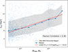 |
Fig. 1 Scatter plot depicting the relationship between the logarithmic halo mass at z = 0 and t1/2 in gigayears for the selected sample of halos from The300. The red line represents the best-fit line that has been obtained by fitting a simple linear relation between the halo mass and the t1/2. |
2.3 BCG and ICL properties
As discussed in the introduction, the t1/2 can be connected to the surrounding BCG area, and, thus, to the ICL. However, a clear separation of the BCG and ICL systems within the halos in both simulations and observations is non-trivial, given that the two components are highly blended. However, a common approach is to employ a fixed aperture radius and consider all the particles within that sphere to identify the BCG region in simulation-based studies or a fixed magnitude limit in observation-based studies. For example, McCarthy et al. (2010) used a 30 h−1 kpc radius aperture, Contreras-Santos et al. (2024) employed a 50 h−1 kpc radius, and Contreras-Santos et al. (2022) used three different aperture radii of 30, 50, and 70 h−1 kpc to define the BCG region. While observers can adopt surface brightness cuts (e.g. Zibetti et al. 2005, and references therein) to separate BCG and ICL. We refer interesting readers to Cui et al. (2014); Presotto et al. (2014); Brough et al. (2024) for comparisons between different separation methods. Following Contreras-Santos et al. (2022), we simply employ three different 3D aperture radii to define the BCG in our halo dataset: 30, 50, and 100 h−1 kpc. The larger radii 100 h−1 kpc information. includes the external wings of the BCG. We select all the gas, stars, black holes, and dark matter particles within the spheres defined by these three different aperture radii to define the BCG region. After defining the BCG, we identify the ICL for our simulated halos by selecting all the star particles that are bound to the halo potential but are not part of either the BCG or any other substructures within the halos. This ensures that the ICL represents stars that are not gravitationally bound to individual galaxy members or merged groups but are instead spread throughout the cluster. Indeed, in general, the ICL covers large portions of the cluster. It is also important to note that ICL used in Table 2 refers to halos where the BCG was determined using a 50 kpc aperture radius 3D cut.
For this, we use the AHF_particles file generated by the AHF, which includes all the IDs of the particles that belong to each halo. After having the BCG and ICL regions identified, we compute their physical properties in order to utilize them within the RF regressor. Using the simulated halo dataset, we first computed the properties corresponding only to the combined BCG and ICL region identified using the 50 h−1 kpc aperture 3D cut which is listed in Table 2. These properties are considered in our RF model as features along with the halo properties computed using AHF (i.e., Table 1). In Table 3, we enumerate all the stellar and gas properties for the BCG defined using three different aperture radii (30, 50, and 100) h−1 kpc for our selected halo dataset from The300 simulated clusters.
After obtaining all the properties associated with the halos and their corresponding BCG regions, we proceeded with data preprocessing. We found four halos with a black hole mass Mbh equal to zero, so we removed these halos from our dataset, including all associated properties from Tables 1, 2, and 3. We also found one halo with an M14 unrealistically high due to there being fewer satellites of satellites, so we removed that halo from our analysis. Finally, we noted that fgas,30 values (defined in Table 3) were not well-defined for two halos, so we excluded them from our analysis as well. Our final halo dataset consists of 1918 halos for which the probability density function (PDF) of their computed t1/2 and histogram of mass distribution is given in Figure 2. It is clear that neither the t1/2 nor the halo mass is uniformly distributed. As presented in previous ML application studies (e.g. de Andres et al. 2022, 2024), the non-uniform property distribution will bias the ML models toward the results with the highest statistics, and thus those studies aimed at creating uniformly distributed datasets to avoid this source of bias. In our study, we implemented a weight to all the following ML training based on the distribution of the t1/2 in Figure 2. While training the various machine learning models, to address the issue of undersampling in the target variable (i.e., very few observations for very early- and late-forming halos, as depicted in the upper panel of Figure 2), we assigned weights to the halos corresponding to the training dataset. We adopted the inverse of the PDF of t1/2 as the weight for each halo with formation time t1/2 in the training set and normalized them so that the sum of all weights is unity. A bump is also noticeable in the mass distribution (Figure 2, lower panel), which arises due to the completeness limit of our sample (see Appendix Cui et al. 2018). Our simulations are zoom-in re-simulations of 324 massive regions identified in the MDPL2 dark matter-only simulation. These regions span a large volume that includes not only the central clusters but also many additional halos. While the halo mass function from the full cosmological volume shows the expected smooth curve, our re-simulated sample becomes incomplete below a certain mass threshold. This incompleteness manifests as the observed bump, marking the mass limit above which our sample reliably includes halos from the full volume.
In the next section, we will explain our analysis that uses the properties described in Tables 1, 2, and 3 to train the random forest regressor to predict the t1/2.
Properties for the BCG and ICL region identified using the 50 h−1 kpc aperture radius for training the RF regressor.
Baryonic properties of the BCG calculated within 30, 50, and 100 h−1 kpc apertures, used to train the RF regressor in this study.
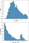 |
Fig. 2 Upper panel: probability density function of the t1/2 values. Lower panel: histogram for the mass distribution for our selected halos sample used in this study. |
3 Random forest regression
The random forest (RF) algorithm (Breiman 2001) is an ensemble-based learning method that combines multiple base learners or regressors to handle multidimensional datasets, offering advantages in solving complex problems and improving model performance. The base learners in the RF algorithm are decision trees, each trained independently of the others during the training procedure. The algorithm utilizes bootstrap sampling with replacement, or bagging, of the original training dataset, which has N rows and M columns. Each tree is trained on a different bootstrap sample. In bagging, each sample consists of the same number of N rows as the original dataset, with some entries potentially repeated and others omitted. Furthermore, each decision tree receives a different set of m features or columns (m < M) from the original dataset, ensuring that the features are not correlated. Each decision tree is constructed using its m subset of features, where the node split in the tree is determined based on the features within the bootstrapped sample extracted from the original training dataset. The node feature and its splitting threshold are decided according to the mean squared error minimization criterion. This process is then executed recursively until we reach a termination condition, such as the maximum depth of the tree or the minimum number of samples per leaf. Once all the decision trees are trained, their predictions are aggregated by averaging the outputs for regression tasks. This aggregation ensures that the final result is robust and not prone to overfitting. For our study, we used the scikit-learn implementation of the random forest regressor (Pedregosa et al. 2011). The algorithm involves several key hyperparameters that need to be tuned to achieve optimal model performance. The important hyperparameters considered in this study for tuning the RF model are listed below, along with their definitions:
n_estimators: This parameter determines the number of decision trees used in the random forest. We considered various values for this parameter.
max_features: This parameter defines the number of subset features, denoted as m (< M-the total number of available features), typically on the order of
 or log2 M.
max_depth: We explored the maximum depth of the decision trees in the RF model.
min_samples_leaf: The minimum number of samples required to be at a leaf node of the decision trees.
The GridSearchCV method within the scikit-learn package is used to tune these hyperparameter values of the RF model. This method works by creating a high-dimensional grid using the range of values for hyperparameters discussed earlier. GridSearchCV then employs K-fold cross-validation, where the training dataset is divided into K equal folds. The K-1 folds are utilized for training, while the remaining fold is reserved for cross-validation. This process is repeated K times, ensuring that each fold serves as a cross-validation dataset. For each coordinate representing a combination of hyperparameters from the high-dimensional grid, GridSearchCV utilizes the training data and evaluates performance using a specified metric (such as accuracy, mean squared error, etc.) through the K-fold cross-validation process described earlier. After evaluating the metric for all combinations in the high-dimensional grid, GridSearchCV selects the best combination of parameters that yields the most optimal performance. In the next subsection, we discuss the training setup we utilized.
3.1 RF training setup
From our sample of halos, we chose 1630 halos (85% of the total) for our training set and 288 halos (15%) for our the test set. This train-test split of the dataset remains fixed throughout to maintain the consistency of the analysis. For the GridSearchCV, the set of values for the hyperparameters is as follows:
n_estimators: [50, 100, 200, 250, 300, 350, 400, 500],
max_features: [
 or log2 M],
max_depth: [6, 7, 8, 10, 13, 15, 17, 19],
min_samples_leaf: [20, 50, 70, 95, 110, 130].
We used GridSearchCV with 5-fold cross-validation with the scoring parameter set to neg_mean_squared_error. The hyperparameter tuning algorithms within the Scikit-Learn package are conventionally implemented to maximize the scoring function; however, for model performance metrics like mean squared error, the objective is to minimize them, as lower values indicate better performance. Therefore, maximizing the neg_mean_squared_error is equivalent to minimizing the mean squared error. The hyperparameter grid and its corresponding search space are utilized to tune the hyperparameters for each RF model individually, which means that each model is optimized separately, resulting in its own set of hyperparameters based on its specific training and validation performance.
Using the aforementioned setup, we applied our halo sample dataset (i.e., Tables 1, 2, and 3) to train the RF regressor algorithm as follows:
Model 1 : RF trained using the properties listed in Table 1 (AHF-computed simulation properties).
Model 2 : RF trained using the properties listed in Table 2 (properties connecting the BCG+ICL region with the halos).
Model 3 : RF trained using the properties listed in Table 3 (stellar and gas properties defined within different 3D radius apertures).
Model 4 : RF trained using the combined properties from both Tables 1 and 2.
Model 5 : RF trained using the combined properties from both Tables 2 and 3.
Model 6 : RF trained using all the properties from Tables 1, 2, and 3.
In the following subsection, we present the results of the RF regression analysis for all six trained RF models listed above.
3.2 RF model results
In this subsection, we present the results of the RF algorithm. We assess the accuracy of the t1/2 predictions against the true t1/2 for the six RF models described above. The results are shown in the left panels of Figure 3. These panels provide a two-dimensional joint density distribution of the true versus RF-predicted t1/2 values, allowing us to investigate the scatter in our predictions relative to the ideal one-to-one model, depicted by a dotted gray line.
Additionally, we quantify the relative error between the RF-predicted t1/2 values and the actual t1/2 values of the test dataset, which is shown on the right panels of Figure 3. The relative error t1/2 values denoted by t1/2 within the plots is defined as (t1/2,True - t1/2,Predicted)/t1/2,True. We first observed that the joint density distribution between the predicted and actual t1/2 values tends to have a different slope relative to the diagonal line, and that the average predicted values are slightly higher than the true ones. This is also evident from the median relative error values, which have a small negative offset from zero in the relative error histogram plot (Figure 3, right panel). This offset from the ideal model is largest for Model 3 (linked to the properties of Table 3) and smallest for Model 2 and Model 4. Thus, by assessing all six models, we infer that they overpredict the actual t1/2 values of the test sample, with a median bias ranging from 4% to 9%.
To further assess the robustness of the RF predictions for our six models, we analyze the joint distribution relative to the diagonal line and the standard deviation of the relative error histogram. A tight clustering of the joint distribution along the diagonal line would indicate high accuracy and low prediction errors. Even though all the models closely follow the diagonal line, the remaining spread suggests that incorporating additional features could further reduce this spread and enhance the accuracy of predictions. The relative error histograms for the six models exhibit variability in the predictions. The standard deviation estimates for the six models indicate that errors in the RF predictions can deviate from the median relative error in the range of 19% to 23%. From Figure 3, we observe that the width of the spread of the joint distribution and the standard deviation of the relative error histogram is lowest for Model 6, which uses all the properties from Tables 1, 2, and 3 for training.
As mentioned in the previous subsection, we incorporated sample weights while training the models to address the undersampling issue at the very low and high ranges of t1/2 values. However, we still observed over-prediction for very early-forming halos and under-prediction for very late-forming halos across all six cases considered in our analysis, attributed to undersampling at those extremes.
During the training of the Random Forest (RF) algorithm, each decision tree is trained using a bootstrapped sample of the training dataset. On average, approximately 63.2% of the original training data is included in the bootstrapped sample for training each tree, while the remaining 36.8%, referred to as out-of-bag (OOB) data, is excluded from the training of that specific tree. For each data point in the OOB sample, a corresponding prediction exists within the OOB_prediction_ array from scikit-learn. This prediction is obtained by aggregating and averaging the predictions from the decision trees within the RF that did not use this data point for training. The OOB prediction data can be used to evaluate the performance metrics of the trained models without the need for a separate validation set.
To further compare the performance of the six RF models, we evaluated and plotted the mean squared error (MSE) for the training dataset, testing dataset, and OOB sample using the predictions from each trained RF model in Figure 4. The plot shows that the mean squared error for the training set for all six models is lower than the test and OOB sample mean squared error, indicating effective training. However, the mean squared error for the training dataset is not drastically lower than the test and OOB sample mean squared error, suggesting minimal overfitting. Overall, for all six models, the mean squared error for the test dataset closely aligns with the mean squared error for the training and OOB datasets, indicating good generalization. Among all the models, Figure 4 illustrates that Model 6, which utilizes all the data from Tables 1, 2, and 3, exhibits a significant reduction in training, testing, and OOB sample mean squared error compared to the other trained models. The OOB MSE is slightly higher than the test dataset MSE due to sampling differences in both methods. The test set predictions use all trees in the forest which leads to a more stable and typically lower MSE. On the other hand, OOB predictions only use the subset of trees that did not see the particular data during training, resulting in a slightly higher MSE due to the smaller and potentially less representative OOB sample.
Lastly, the importance of each feature for the six models we trained in our study was determined using the scikit-learn permutation_importance function Breiman (2001). The algorithm works by first calculating the baseline performance of the model using a metric (such as mean squared error) on the dataset. We then select one feature at a time and permute its values to break any relationship between the feature and the target values. The model is then evaluated with the shuffled feature, and its performance is compared to the baseline model performance to gauge the importance of the feature. This process is applied recursively to all the features in the dataset. In Figure 5, we display the permutation feature importance of the six models considered in this study. The first thing we notice from Figure 5 is that the most important feature is overall the com_offset of the halo, for which we found a strong positive correlation with the t1/2, with a Pearson’s correlation coefficient value of 0.63. The com_offset is an indicator of the dynamical state of the halo (Ludlow et al. 2012; Mann & Ebeling 2012) and, it’s known that relaxed halos tend to assemble their mass earlier compared to unrelaxed ones (see, e.g., Mostoghiu et al. 2019; Power et al. 2012, for more discussion on the correlation between a halo’s dynamical state and its formation time). Following, the other important properties contributing to the statistical performance of Model 6 are M12, MBCG/Msat, M14, meanZ*, Mbh, and so on. We observe a strong negative correlation between the magnitude gaps (M1,2, M1,4) and t1/2, with Pearson’s correlation coefficients of −0.63 for M12 and −0.56 for M14, respectively. As discussed in the introduction, that trend was expected since the hierarchical growth of the BCG can induce a change in the magnitude gap M12 or M14 which could serve as an indicator of t1/2 (Golden-Marx & Miller 2018, 2019; Golden-Marx et al. 2022, 2025). We also note here that the mass gap (or magnitude gap in observations) is also strongly anti-correlated with the com_offset, and has been used as a parameter for quantifying the halo dynamical state.
We have so far utilized halo properties extracted from AHF (Table 1), properties corresponding to the BCG-ICL region (Table 2), and stellar and gas properties of the BCG at different aperture cuts (Table 3) to fit the RF models for predicting t1/2. The analysis of the six random forest models in this section shows that the random forest algorithm can indeed predict the formation time of the halos and the model’s prediction accuracy extensively improves as we incorporate more features into the model However, the feature importance plot in Figure 5 also indicates that not all properties play an important role in predicting t1/2. Therefore, instead of naively expanding our feature space by including all possible properties, in the next section, we will focus on using the BCG properties that can be computed from observations. This approach reduces the complexity of our RF model by narrowing down our feature space.
Moreover, when defining the BCG region, we discussed how the radial aperture size used to define the BCG is selected arbitrarily in different literature, and in this study, we utilized three different aperture radii to compute the BCG’s stellar and gas properties, all of which are detailed in Table 3. However, if the chosen aperture radius is too small, we may miss the region that is more important for predicting t1/2. On the other hand, though f*,100 is the most important feature in Model 3 as expected, choosing a larger aperture might introduce a lot of unimportant information, which could overshadow the region most helpful in predicting t1/2. To derive the most important and clean information for t1/2 around the BCG as suggested by Golden-Marx et al. (2022, 2025), in the next section, we will utilize different CNN models that rely solely on the stellar and gas properties of the BCG region for each halo in our dataset. After training these CNN models, we will use them to identify robust radial aperture ranges for each BCG baryonic property that most strongly correlates with the formation time of the halos. Using the identified aperture ranges for the baryonic properties from the CNN models’ results, we can directly compute these properties and train random forest models with features selected based on prior informed decisions rather than using them arbitrarily.
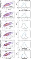 |
Fig. 3 Left panel: relationship between the true and the predicted t1/2 values using the six trained RF models through a bi-variate joint distribution or 2D probability density function. The black data points represent the scatter between the RF predictions and the true t1/2 values for the test dataset relative to the ideal case of perfect predictions, depicted by a 45-degree dotted gray diagonal line. Right panel: probability density function for the relative errors between the true t1/2 and the predicted values by the RF models, along with the median error and the standard deviation, 1σ. |
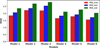 |
Fig. 4 Mean squared error (MSE) for the training, test, and out-of-bag samples for the six models trained using the RF algorithm to assess the model performance. |
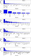 |
Fig. 5 Permutation importance of the features in the six different random forest regressor models we considered in this study. |
4 Convolutional neural networks
Convolutional neural networks (CNNs; LeCun et al. 1998, 2015, for a detailed review see Aloysius & Geetha 2017) are a class of artificial neural networks (ANNs) commonly used for imagebased machine learning problems, where the typical input to the network involves two-dimensional image data. In contrast to traditional ANNs, where each neuron in a layer is interconnected to every neuron in the previous layer, CNNs first process the input image through layers dedicated to convolution and pooling operations, which are subsequently followed by fully connected layers of neurons. A single convolutional layer of a CNN consists of multiple kernels, each having a lower dimensionality than the input data. As these kernels traverse the image, they perform convolution by calculating the scalar product between the filter elements and the corresponding input elements, thereby generating a feature map. The kernels are responsible for extracting patterns from the input two-dimensional data, such as horizontal and vertical textures. The components within each kernel constitute a set of weights that are fine-tuned during the CNN training process.
The generated feature map is then activated by an elementwise activation function, such as the rectified linear unit (ReLU, Nair & Hinton 2010), which introduces non-linearity into the CNN, enabling the model to learn complex patterns. Mathematically, RELU is defined as f(x) = max(0, x), which ensures that all negative values (representing black pixels) are ignored, preserving only positive values (corresponding to gray and white pixels).
The activated feature map from the convolutional layer is then processed by the pooling layer, which reduces the dimensionality of the feature map while retaining the most important information. This is typically achieved by applying either max pooling or average pooling. In the case of max-pooling, the operation extracts the maximum element from the area of the feature map covered by the pooling filter, whereas, in average pooling, it calculates the average of all elements in the region of the feature map covered by the pooling filter. As the feature map passes through convolutional pooling layers, it extracts larger features and reduces in size, cutting computational costs while retaining key information. The output is then flattened to a onedimensional layer for fully connected layers. The final output can be a single neuron for binary classification or regression, or multiple neurons for multiclass classification.
The network consists of several hyperparameters that can be tuned to achieve optimal performance. We only considered three hyperparameters in our study, which are as follows:
epochs : It refers to the number of complete passes of the training dataset through the model. One complete pass involves processing the data set forward and backward through the network once, ensuring that the model has seen and learned from every training example exactly once.
learning rate: It specifies the magnitude of the step taken in the parameter space by the optimization algorithm while adjusting the weights of the CNN during the training process.
dropout rate: It is a regularization technique that prevents overfitting in the model by ignoring some neurons in the fully connected layer. The dropout rate represents the fraction of neurons that will be randomly ignored during training.
In the next subsection, we detail the creation of input maps/images for the training, the CNN architecture, and the optimization hyperparameters.
4.1 CNN architecture and training Setup
An initial prerequisite for using a CNN is the input image data. We first derived property maps for the halos used in the RF analysis, which are used as input images for training the CNN network. The training and test samples from the RF study were used directly, meaning no new train-test split was created. To produce property maps, we considered the stellar and gas properties of the halos, which were computed based on their respective particle information within the simulation. The properties we considered include: (i) mass-weighted stellar metallicity (Z*), (ii) mass-weighted stellar age (tage), (iii) stellar mass (M*), (iv) gas mass (Mgas), (v) mass-weighted gas metallicity (Zgas), and (vi) mass-weighted gas temperature (Tgas), which were computed using the information of the stellar and gas particles within the simulated halos. For each halo, the gas and stellar particles were binned into forty uniformly distributed bins in three different ranges of radial distances, explained below.
The six properties stated before were calculated within each bin to generate a property map of size 6 × 40. We note that only the particles belonging to the halo, and not any subhalos within it, are considered for creating these property maps. The three different methods used in this study for binning the stellar and gas particles are as follows:
Binning Method 1: 40 uniformly spaced bins defined from the center to 650 kpc physical distance to ensure a consistent particle distribution.
Binning Method 2: 40 uniformly spaced bins defined from the halo center to a radius of 0.3 × R200c.
Binning Method 3: 40 uniformly spaced bins defined from the center of the halo to 16 × Rhalf, fit, where Rhalf, fit is the half-stellar mass radius of the central galaxy within the halo. The Rhalf, fit values for our halo dataset are based on the CAESAR catalog. However, the CAESAR catalog’s radius estimations showed a significant scatter for a fixed value of stellar mass within the half-stellar mass radius (i.e., M*,half), with a deviation of approximately 8.78 kpc from the best linear fit, which results in the ML prediction with very large scatter. Therefore, we used the half-mass radius values predicted by the linear fit relation between the M*,half and Rhalf of the CAESAR catalog.
The bin positions within the map for each halo in the first binning method are always normalized to the maximum bin edge, i.e., 650 kpcs. In the latter two cases, they are normalized to their corresponding R200c and Rhalf, fit, to place all the halos used in the analysis on equal footing. In Appendix A, we present the distribution of 0.3 × R200c and 16 × Rhalf,fit for all the halos in Figure A.1 to give an idea about the average spatial resolution of the Binning Method 1 and Binning Method 2. The maps developed for each halo correspond to a 2D image, where each vertical slice of the property map represents a bin and consists of six vertical columns of pixels, with their pixel values corresponding to the stellar and gas properties of the halo within that bin. For some halos, we noticed that gas properties were computed as NAN due to the absence of gas particles within the bins. We excluded those bins from the property maps so that it does not lead to CNN training failure. We could not ignore the halos with this issue because a few bins (1 or 2) with NaN values occur frequently in some halos within our dataset. If we ignored these halos, our sample size would become very small, making it unsuitable for training the CNN network. However, they are resized later on to have the same dimensions to make CNN training possible. Also, the numerical value ranges for the six physical properties in each row can vary widely. This leads to pixel value distributions that differ significantly between properties. In our case, the gas temperature, stellar mass, and gas mass values are considerably larger than the other three properties, causing these three properties to overshadow the rest. We applied transformations to these maps to ensure that the magnitude range difference between the six properties does not impact the CNN training and that each property’s overall distribution across all maps in the combined training and test sets is close enough to a normal distribution. A base-10 logarithmic transformation was applied to compress the large magnitudes of the gas temperature, stellar mass, and gas mass within the property maps. The gas metallicity values within the bins across all the maps in the training and testing data set are between 0 and 0.075 and the distribution for it is very squeezed for the smaller values range. Therefore, to expand the distribution and to make it more distinct, we performed a square root transformation over all the values of gas metallicity. The stellar age values were transformed using:
 (1)
(1)
where max(tage) represents the maximum stellar age across all the maps, i.e., after concatenating the whole training and testing map datasets. This transformation ensures that the overall distribution of stellar age values is not skewed toward the tail end and approximately follows a normal distribution. No transformation was applied to the stellar metallicity data within the map. Finally, after applying the transformations to the individual physical properties of the maps, we applied Z-score normalization to each property. The Z-score normalization is mathematically expressed as:
 (2)
(2)
where p corresponds to one of the six physical properties used in the maps. Xp represents the original value of property p, while Xp is the normalized value. μp and σp are the mean and standard deviation of property p, calculated across the entire dataset by combining all the maps from the training and test sets. The Z-score normalization scales the data with a mean of zero and a standard deviation of one, ensuring that each feature or property is placed on equal footing, regardless of the scale of the original data. All the maps are then resized using OpenCV (Bradski 2000) to have the dimensionality of 6 × 40 so that the input map sizes for CNN training are consistent. Like the halo dataset from the random forest analysis, we now possess 1630 property maps in the training dataset and 288 in the testing dataset. In Figure 6, we present the property map for a halo using the three different binning methods, with all normalization, and Z-score standardization applied to each row or property within the map.
After computing these maps for the halo dataset, we designed our network to use these property maps to make t1/2 predictions. We implemented our CNN architecture using the Keras package with TensorFlow backend, written in Python. The architecture of our ‘single-channel’ CNN is as follows:
-
Convolutional-Pooling Layer 1
1 × 3 convolution, 64 filters, with ReLU activation
1 × 2 stride-2 max pooling
-
Convolutional-Pooling Layer 2
1 × 3 convolution, 64 filters, with ReLU activation. The padding is set to ‘same’ so that the output feature map has the same spatial dimensions as the previous layer feature map.
1 × 2 stride-2 max pooling
Flattening Layer
-
Dense Layer 1
128 neurons, fully connected followed by activation function set to ReLU
-
Dense Layer 2
64 neurons, fully connected followed by activation function set to ReLU
Output Layer The final output layer uses the linear activation function.
We chose 1D vector kernels for convolution and pooling operations rather than 2D kernels because different rows in the input maps correspond to different physical quantities which are independent of each other, and we do not want them to convolve with each other by using 2D kernels either. In Figure 7, we give the pictorial representation of our ‘single channel’ CNN network. Instead of using different CNN architectures for each of the three binning methods, we used the same architecture to see how the predictions are affected by binning gas and stellar particles using different criteria. We trained three CNN models, which are as follows:
CNN Model 1 : CNN trained using input training maps generated with Binning Method 1.
CNN Model 2 : CNN trained using input training maps generated with Binning Method 2.
CNN Model 3 : CNN trained using input training maps generated with Binning Method 3.
The range of values for the hyperparameters we consider are as follows:
epochs : [17, 21, 31, 41, 49]
dropout rate : [0.1, 0.2, 0.3, 0.4, 0.5]
learning rate : [10−5, 10−4, 10−3, 10−2, 10−1].
To tune the hyperparameters of these CNN models, we used GridSearchCV again with five-fold cross-validation. We used the Adam Optimizer (Kingma & Ba 2014) with a mean squared error loss function during the training of our CNN model. The training data were divided into batches of 51 training maps each. The weighting criteria based on the distribution of t1/2 in Figure 2 are also applied again during the training of the CNN models.
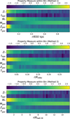 |
Fig. 6 Property maps for a halo with R200c = 1035.84 kpc/h and |

4.2 CNN results
Our predictions for halo formation times in the test set for the three different binning methodologies are shown in Figure 8. The left column of the figure presents scatter plots comparing the CNN-predicted t1/2 to the true t1/2 for each of the three binning criteria. The contour plot illustrates the 2D joint density distribution of the CNN-predicted and true t1/2 values for the test set. The right column contains histogram plots showing the relative error between the CNN predictions and the true t1/2 values, again for the three different binning methodologies used to create the maps for the halo dataset.
We infer from the relative error histograms for CNN Model 1 and CNN Model 3 that the model overestimates the formation time values, with median relative error biases of 4.1% and 0.4%, respectively. This is low compared to all the random forest models discussed in Section 3. On the other hand, the predictions for the CNN Model 2 underestimate the formation time values, with a median relative error bias of 1.6%. We see that the median relative error bias is the lowest for the CNN model 3 where the input maps for training and testing are generated following binning Methodology 3, i.e., 40 uniform bins located between 0 to 16 × Rhalf,fit.
However, the scatter of the relative errors for the CNN predictions is slightly larger compared to all the random forest models investigated in Section 3.2. The same can be inferred from the width of the 2D joint distribution in the left panel plots for all three methods in Figure 8. The scatter in the relative errors of t1/2 predictions from median relative errors is the lowest for CNN Model 2, where the maps are generated by binning the gas and stellar particles within 40 uniformly spaced bins from 0 to 0.3 × R200c. Another contrast in the CNN models’ relative error histogram compared to the RF models’ is that the left tail of the CNN models’ histogram is skewed, implying that the CNN models tend to overpredict the formation time values by relatively large errors. The promising aspect, however, is that with just six observable properties around the central galaxy hosted within the dark matter halo-thereby reducing our feature space-we can achieve predictions with a reduced median relative error bias, though with a scatter that is only 25% larger compared to the random forest models.
Additionally, we interpreted the CNN models using saliency maps and analyzed them to identify the radial range that exhibits the strongest correlation with galaxy properties, enabling its direct incorporation into a machine-learning model for estimating the halo formation time. However, we did not include the saliency maps analysis in the main section of the manuscript, as the saliency maps are not easily interpretable due to the high correlation between features in different bins and their generally low correlation with t1/2 itself at different radii. An extensive discussion of the saliency maps for the three CNN models trained in this section is provided in Appendix B.
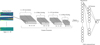 |
Fig. 7 Architecture of the “single-channel” CNN used in our study. Our network employs two convolutional pooling layers for feature extraction and two fully connected layers for parameter estimation. |
5 Benchmarking the RF and CNN models
In this section, we assess the performance of the RF and CNN models in reproducing the key correlation trends between t1/2 and both M200c and cNFW, as well as evaluate the accuracy of their predictions against halo formation time estimates derived from analytical approaches, such as that of Correa et al. (2015).
We begin by examining the correlation between the predicted t1/2 and the halo mass M200c. The true relation has already been discussed in Figure 1. As shown in Figure 9, all six RF and three CNN models successfully reproduce the expected positive trend between M200c and t1/2. The median binned relations from the ML-predicted t1/2 values, denoted by red lines in all panels of Figure 9, align closely with those derived from the true simulation values, shown with dotted black lines. Moreover, the associated ±34 percentile scatter range shows significant overlap, as the red shaded regions for the ML predictions coincide with the gray regions representing the simulation percentile range as shown in Figure 9. This consistency suggests that the models are effectively capturing the underlying physical correlation. Quantitatively, the overall Pearson correlation coefficient between M200c and the predicted t1/2 is 0.39, with the RF models achieving a mean correlation of ~0.52, and the CNN models ~0.46. We would also like to emphasize that the halo formation time predicted scatter from the ML models is relatively underestimated compared to the true scatter. This is expected from ML models trained with the MSE loss function, which is known to favor mean predictions and suppress variability in the tails of the target distribution. This is also reflected in the larger correlation coefficient (i.e., reduced scatter) between the predicted formation time and mass, compared to the true formation time and mass.
Turning to the halo concentration parameter cNFW, we find a clear negative correlation with the true t1/2 of the simulated halo dataset, as shown in Figure 10. This is consistent with the expectations from hierarchical structure formation, where earlier-forming halos tend to be more concentrated than their late-forming counterparts. As illustrated in Figure 11, both the RF and CNN models successfully reproduce the expected negative correlation between t1/2 and cNFW. The true simulationbased correlation is −0.22, while the RF and CNN models yield mean correlations of approximately −0.20 and −0.17, respectively. Similar to the case of M200c, the predicted median trends closely follow the actual median trend, and the percentile ranges largely overlap with those derived from the true values. This indicates that the machine learning models are capable of recovering this inverse relationship.
We also benchmarked the performance of our ML models by comparing the predicted t1/2 values with those obtained from an analytical approach based on the extended Press-Schechter (EPS) theory, specifically following the formulation presented in Correa et al. (2015). This assessment was conducted using the M200c-t1/2 relation shown in Figure 9. The 16th-84th percentile gray shaded region in Figure 9, derived from the simulationbased t1/2 values, was obtained by tracing the mass accretion histories of halos through merger trees constructed using AHF. These simulation-based formation times exhibit significant scatter when compared with t1/2 values calculated using the commah3 package. This package given in Correa et al. (2015) implements the analytical framework for modeling the mass accretion histories of halos, from which t1/2 can be computed. The scatter of the simulation data relative to the green line-representing the analytical formalism-highlights the diversity in halo assembly histories: halos of the same mass can have significantly different formation times. Nonetheless, the median trend of the simulation-based t1/2 values broadly follows the analytical predictions for halos of lower masses. However, at the high-mass end, the simulation data predict later formation times than the analytical model. The RF and CNN model predictions show a similar trend and generally follow the simulation results: at lower halo masses, the predicted t1/2 values align well with the analytical estimates, while at higher masses, they diverge, indicating later formation times. However, the RF predictions deviate more strongly from the analytical model than the simulation data, in contrast to the CNN models. Although the CNN predictions also exhibit divergence at high masses, the extent of this deviation is smaller than that seen in the RF models. We would also like to highlight that the formation time predictions from our machine learning models-particularly the CNNs-are made on a per-halo basis using only information from the cluster at redshift z = 0. In contrast, the analytical formalism of Correa et al. (2015) provides only a median trend. As a result, our approach better captures the scatter and yields higher accuracy, especially for cluster-sized halos. Overall, this comparison reinforces that both RF and CNN models effectively learn the physical trends of halo assembly from the simulations.
 |
Fig. 8 Predictions of the halo formation time (t1/2) and corresponding accuracy assessment for the three CNN models. Left panel: scatter plots (black points) showing the true versus predicted t1/2 values for the test dataset. Contour lines indicate the joint two-dimensional distribution, and the dashed 45-degree line represents perfect prediction. Right panel: probability density functions of the relative errors between predicted and true t1/2 values, showing the median and standard deviation (1σ) for each model. |
6 Linear models for halo formation time estimation
In this section, we aim to construct simple linear models that are less complex than CNN and RF models while providing a reasonable estimate of t1/2 without introducing the complexities inherent in advanced machine learning models.
We begin by building a linear model4 to infer t1/2 using only the magnitude/mass gap M12, which represents the logarithmic mass difference between the total BCG mass, defined within a 50 h−1 kpc 3D aperture, and the most massive substructure. As highlighted in the introduction and the feature importance analysis of Model 2, Model 4, and Model 6 of the random forest (discussed in Section 3.2), the magnitude gap is a robust indicator of t1/2 (Golden-Marx & Miller 2018, 2019; Golden-Marx et al. 2022, 2025). Since this quantity can be computed observationally, it provides a practical means of estimating t1/2.
In the first panel of Figure 12, we present the t1/2 prediction analysis for the halos in the test set based on a linear model trained using M12 values from the training dataset. The training and test datasets are the same as those used previously. This model yields a reasonably accurate estimate of t1/2, with a median relative error that slightly over-predicts values by 4.6 percent and a scatter of 0.271 in the relative error, indicating a moderate spread in predictions. The simple linear relation can be expressed as
 (3)
(3)
We further refine this linear model by incrementally incorporating additional properties from the set of observable features listed in Tables 2 and 3 in Section 2. The goal is to reduce the scatter and median relative error bias in the M12-t1/2 relation by integrating more relevant observational properties.
In the second panel of Figure 12, we introduce a refined linear model that incorporates MBCG/Msat alongside M12. The selection of this additional feature is guided by the feature importance plots in Figure 5 and a systematic brute-force approach, where each property from Tables 2 and 3 was tested individually to determine its effect in terms of performance of the M12-t1/2 relation. Among the tested properties, MBCG/Msat yielded the best performance in terms of median relative error, bias, and scatter.
The choice of MBCG/Msat was based not only on performance improvements but also on its correlation with both M12 and t1/2. While MBCG/Msat shares some information with M12, it still entails a distinct aspect of the cluster’s properties that influences the linear model’s performance, as seen in Figure 5. With the inclusion of MBCG/Msat, the scatter in the relative error histogram is reduced to 0.264, and the median overestimation bias decreases to 3.5%, marking an improvement of approximately 1.1% over the single-feature model. This refined linear model is expressed as:
 (4)
(4)
where the definitions of M12 and MBCG/Msat are provided in Table 2.
In the third panel of Figure 12, we present a further improved linear model that builds upon the previous version by incorporating an additional mass gap, M14, as defined in Table 2. The inclusion of M14 follows the same brute-force approach, where different observables were tested individually for their impact on the M12-t1/2 relation. By adding M14, the model reduces the scatter in the relative error to 0.251 while slightly increasing the median overestimation bias to 5.3%, an increase of 0.7% compared to using M12 alone. The final linear model is given by:
 (5)
(5)
where the definitions of M12, MBCG/Msat, and M14 are provided in Table 2. Lastly, we have also verified that including the com_offset only marginally improves the linear models by reducing the scatter. This is because the com_offset is tightly correlated with M12. For the sake of simplicity, we did not include this information in these linear models.
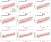 |
Fig. 9 Correlation between the halo mass M200c and t1/2 across different RF and CNN models. The first and second rows show the correlation trends for the six RF models discussed in Section 3, while the third row corresponds to the three CNN models described in Section 4. In each panel, the shaded red region represents the 16th-84th percentile range of the ML predictions, and the shaded gray region shows the same range for the actual simulation values. The solid red and dotted black lines indicate the median t1/2 in logarithmic mass bins for the ML models and the simulation, respectively. Pearson correlation coefficients are annotated to quantify the strength of the relationship between M200c and the predicted formation times. The solid green line gives the t1/2 - M200c relation based on formation time values calculated using the analytical formalism based on EPS theory as given in Correa et al. (2015). |
 |
Fig. 10 Scatter plot depicting the relation between the concentration parameter cNFW and t1/2 in Gyr for selected sample of halos from The300. The red line depicts the best-fit line obtained by fitting a simple linear relationship between cNFW and t1/2. |
7 Conclusions
In this paper, we developed machine learning models to predict t1/2 using theoretical and observationally motivated properties derived from The300 Gizmo-Simba simulations. From these simulations, we extracted 1918 dark matter halos within a broad mass range of 2.50 × 10¹³h−1M⊙ - 2.64 × 10¹⁵h−1M⊙ using AHF halo catalogs. The formation time for these halos, defined as the epoch at which a halo accretes half of its final mass, was computed using halo merger trees constructed with the MERGERTREE tool within AHF.
Our random forest models demonstrated that t1/2 predictions can achieve high accuracy by capturing non-linear relationships between halo formation time and various properties, including halo properties (Table 1), BCG-ICL properties (Table 2), and gas and stellar properties (Table 3). Among the six models shown in Figure 3, Model 6, which utilized all available features, achieved the best balance between bias and the lowest variability in relative error, emphasizing the importance of comprehensive property inclusion. The feature importance plots in Figure 5 highlighted properties such as com_offset, M12, and followed by others as crucial for prediction accuracy. We refer the reader to Figure 5 for a complete description of the important features.
To focus on properties that are more observationally driven and directly aid in predicting t1/2, we trained CNNs using six baryonic properties: Z, tage, M, Mgas, Zgas, and Tgas. Using three different halo property map datasets-each based on a distinct binning strategy-we trained three separate CNN models with the architecture shown in Figure 7 to examine how binning methodology affects t1/2 predictions. The CNN models exhibited slightly lower bias in t1/2 predictions compared to random forest models; however, the scatter in relative prediction error was approximately 5% higher (see Figure 8). Based on the CNN results, we defined optimal radial ranges for each property (listed in Table B.1 for all three binning approaches), which enabled the training of simplified random forest models. These targeted models showed slightly reduced accuracy compared to the CNNs but performed robustly, achieving biases of 7.3-9.7% with manageable scatter in the relative prediction error, highlighting the robustness of CNN-informed feature selection. We further investigated in 5 the performance of the RF and CNN models in reproducing key correlation trends, such as M200c - t1/2 and cNFW - t1/2, and also assessed how the performance of the ML models compares to the analytical formalism of Correa et al. (2015). The RF and CNN models successfully reproduce the key correlation trends between t1/2 and properties such as M200c and cNFW. Benchmarking against both simulation-based formation times and the analytical formalism shows that the models capture the underlying physical trends more closely to the simulation, i.e., the actual truth, and demonstrate that both RF and CNN models effectively learn to predict the formation time of the halos.
Finally, we developed three simple linear models using key observable properties from Tables 2 and 3, achieving competitive accuracy while reducing the complexity of CNN and RF models. These linear models provide a practical framework for observers to estimate t1/2 directly. The baseline model, which uses only M12, has a median overestimation bias of 4.6% and a scatter of 0.271. Adding observable properties such as the ratio of the total BCG stellar mass to the total satellite stellar mass within the halo (MBCG/Msat) and the magnitude/mass gap (M14) further improves the scatter while maintaining accuracy. The linear model incorporating both M12 and MBCG/Msat reduces the scatter to 0.264 with a 3.5% bias, while the model including M12, MBCG/Msat, and M14 further decreases the scatter to 0.251 with a 5.3% bias. We also provide the mathematical relations for these three linear models in Equations (3), (4), and (5), allowing observers to directly estimate t1/2. Although these models slightly increase the median relative error bias in predicting t1/2, they strike a good balance by capturing essential information in a simpler form, reducing model complexity without sacrificing predictive quality. The practical application of these linear models depends largely on the observational context. Although t1/2 is a theoretical quantity derived from simulations and cannot be directly measured in observations, these relations can serve as useful approximations by employing observable proxies. For instance, in optical surveys such as those conducted with HST, quantities like the magnitude gaps M12 and M14, as well as the mass ratio MBCG/Msat, are relatively straightforward to determine-though some level of scatter in the inferred t1/2 is expected. Interestingly, the fBCG+ICL fraction, which is suggested to correlate strongly with halo formation time by Kimmig et al. (2025), does not pop up in our studies, indicated as f*,100. Though there are some differences to the fBCG+ICL fraction, and it is the most important feature in our Model 3 (see Figure 5), compared to other quantities, f*,100 is much less significant. One simple explanation is that this quantity is strongly correlated with the other important features. This is also supported by both observation (Jiménez-Teja et al. 2018) and simulation (Contreras-Santos et al. 2024) results - the dynamical relaxed clusters tend to have lower ICL fraction compared to these unrelaxed clusters.
This study highlights the potential of combining machine learning to refine halo property predictions, reducing model complexity while preserving accuracy. However, the results are specific to simulations using Gizmo-Simba physics. Future work will explore the impact of varying baryonic physics on the prediction performance.
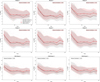 |
Fig. 11 Correlation between the halo concentration parameter cNFW and t1/2 across different RF and CNN models. The first and second rows show the correlation trends for the six RF models discussed in Section 3, while the third row corresponds to the three CNN models described in Section 4. In each panel, the shaded red region represents the 16th-84th percentile range of the ML predictions, and the shaded gray region shows the same range for the actual simulation values. The solid red and dotted black lines indicate the median t1/2 in logarithmic bins for the ML models and the simulation, respectively. Pearson correlation coefficients are annotated to quantify the strength of the relationship between cNFW and the predicted formation times. |
 |
Fig. 12 The first panel compares the t1/2 predictions with the actual values for the test dataset using a linear model based solely on the magnitude gap M12. The second and third panels show the linear model predictions when additional observable properties from Tables 2 and 3 in Section 2 are incrementally included, namely MBCG/Msat and M14, along with M12. The second panel presents predictions analysis from a linear model using MBCG/Msat along with M12. Similarly, the third panel show predictions analysis based on MBCG/Msat and M14, respectively, combined with M12. In the right column, we show the usual scatter and contour density plots comparing the predicted and actual t1/2s, while the histogram of relative errors is displayed on the right side. We also present the relative error histogram for CNN Model 2, which provides the best balance between median relative error bias (positive median bias) and scatter among the three CNN models. This is for comparing the performance of the linear models with that of the CNN models. |
Acknowledgements
AS and WC are supported by the Atracción de Talento Contract no. 2020-T1/TIC-19882 granted by the Comunidad de Madrid in Spain. WC also thanks the Agencia Estatal de Investigaciôn (AEI) for the Consoli-dación Investigadora Grant CNS2024-154838, the science research grants from the China Manned Space Project and HORIZON EUROPE Marie Sklodowska-Curie Actions for supporting the LACEGAL-III project with grant number 101086388. WC and DdA thank the Ministerio de Ciencia e Innovaciôn (Spain) for financial support under Project grant PID2021-122603NB-C21. ER acknowledges support from the Chandra Theory Program (TM4-25006X) awarded from the Chandra X-ray Center which is operated by the Smithsonian Astrophysical Observatory for and on behalf of NASA under contract NAS8-03060. YZ is supported by the National Key Basic Research and Development Program of China (No. 2023YFA1607800, 2023YFA1607804), the National Science Foundation of China (12173024), the China Manned Space Project (No. CMS-CSST-2021-A01, CMS-CSST-2021-A02, CMS-CSST-2021-B01), the “111” project of the Ministry of Education under grant No. B20019, and the generous sponsorship from Yangyang Development Fund. The work presented here emerged out of the annual The300 workshop held at UAM’s La Cristalera during the week July 8-12, 2024, partially funded by the ‘Ayuda para la Organizaciôn de Jornadas Cientificas en la UAM en el Marco del Programa Propio de Investigación y con el Apoyo del Consejo Social de la UAM’ The authors acknowledge The Red Española de Supercomputación for granting computing time for running the hydrodynamic simulations of The300 galaxy cluster project in the Marenostrum supercomputer at the Barcelona Supercomputing Center.
Appendix A Histograms of the maximum bin Edges for the halo sample
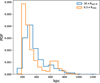 |
Fig. A.1 Histograms showing the distribution of 0.3R200c and 16Rhalf,fit for the halos used in this study. In Figure A.1, we show the distributions of 0.3 × R200c and 16 × Rhalf,fit for the halos, representing the maximum edges of the bins used to construct property maps with Binning Methodology 2 and Binning Methodology 3. |
Appendix B Saliency maps
B.1 Interpreting CNN performance and identifying key property aperture ranges
Understanding the results of CNNs and other deep learning models is challenging due to their high complexity, which stems from billions of interconnected parameters within the network. These parameters exhibit complex, non-linear relationships with each other, making it difficult to understand how each parameter influences the final output. This complexity further complicates the process of deriving clear insights from their outputs. Moreover, the network employs a series of activation functions from one layer to the next, which are not straightforward to interpret, and thus hinder the ability to trace the path from input to final output in the network. That is why CNN models are popularly known as ’black boxes’ due to these complexities. Many methods are currently being devised to enhance the interpretability of CNN networks. In this subsection, we attempt to interpret our singlechannel CNN network using the pixel attribution methodology discussed in Molnar (2020) to understand the contribution of each pixel in the input image to the prediction. We achieve this by employing the Vanilla Gradient-based approach introduced in Simonyan et al. (2013). This method works by forward propagating the image of interest through the network, then computing the pixel-wise gradient of the loss to the input image using the back-propagation algorithm, where the pixel values indicate how sensitive the model’s output is to changes in the input features.
During the CNN training, we back-propagated each property map from the training and test set through the network to generate the saliency map with dimensionality the same as the input property map. The pixel values in each saliency map were then normalized between 0 and 1. The saliency maps for each halo were then stacked together to form the final map that contains statistical information on the region that significantly impacts the network prediction. In the upper panel of Figures B.1, B.2, and B.3, we present the final stacked saliency maps obtained from CNN Model 1, CNN Model 2, and CNN Model 3, respectively. The saliency maps obtained from the three CNN models highlight how variations in the training input maps, resulting from different binning criteria, affect the network’s interpretability. It is clear that these highlighted regions as indicated by the color bar on top have a higher effect on the CNN’s predictions: M*, Mgas and Zgas for model 1; Mgas and Zgas for Model 2; M*, Mgas and Tgas for model 3. The significance of stellar mass in predicting the assembly history of the halo has been suggested in various studies, such as Yang et al. (2006),Lin et al. (2016), Lim et al. (2016). However, the saliency maps from different models give different predictions, not only the properties but also their positions, which are detailed in the following paragraph.
In the lower panels of Figures B.1, B.2, and B.3, we show the profiles of the saliency maps for all six properties. To determine the most significant aperture range for each CNN model/binning methodology, which is used later for a simpler model to predict the t1/2, we identified the position where the pixel value is at its maximum. From this maximum position, we expanded the area by 10% of the total area under the curve above and below this position to obtain the upper and lower radial bounds corresponding to each property in the saliency map. Slightly increasing or decreasing this range has a very minor effect on the model’s prediction power. In the lower panel of Figure B.1, the identified aperture ranges for the six properties of CNN Model 1 are shown as shaded gray regions, and these ranges are listed in the first column of Table B.1. From the distribution plots of CNN Model 1, we can see that identifying the regions to consider is not as straightforward. For example, the M* distribution shows two nearly identical peaks, indicating that both regions are equally important for this property. The same can be stated for Z*, where we find nearly three identical peaks. The aperture ranges for the six properties of CNN Model 2, as identified in the lower panel of Figure B.2, are listed in the second column of Table B.1. We note that the most important property for CNN Model 2 is gas mass. The halos vary significantly in size, with more massive halos having larger R200c. This differs from binning based on a fixed distance of 650 kpc, which may not be able to fully probe the interior regions of massive halos when the same bin is applied at different positions for halos of varying mass. Model 2 appears to yield more consistent results, as quantities in bins that scale with R200c are on equal footing for halos of different sizes, meaning the quantities are estimated relative to each halo’s size. However, such estimations rely on accurately measuring R200c, which is not straightforward to determine from observations. Finally, the aperture ranges for the six properties for model 3 are shown in the lower panel of Figure B.3, with their radii ranges listed in the third column of Table B.1. The most important property in this case is the stellar mass. Similar to the saliency map for binning Method 1, also this map is noisier compared to the saliency map of Method 2 (i.e., Figure B.2).
The aperture ranges for almost all the properties, as estimated using a stacked saliency map for the three different CNN models, indicate that the region the network deems most important lies well beyond the BCG region, plus the area beyond the transitional radius (i.e., the distance where the ICL starts to dominate the BCG stellar component), especially for CNN Model 1. Various literature sources have reported estimates for this transition radius, which vary depending on the methodologies employed to identify the ICL. Observational studies have found this range to be 60-80 kpc (Montes et al. 2021), with slightly increased values reported by Zhang et al. (2019) at 100 kpc, and Chen et al. (2022) at 70-200 kpc. Conversely, Contini & Gu (2021); Contini (2021); Contini et al. (2022) used numerical simulations to show that the transition radius is 60 ± 40 kpc. In our study, this best radius range for predicting the t1/2 depends on the binning method as well as on the baryonic properties, i.e. the proposed transition radius from observations may not be the best indicator for t1/2.
Radius ranges selected from saliency maps for six key properties.
B.2 Random forest model using properties calculated within aperture ranges
We used the saliency ranges of the properties listed in Table B.1 from the three CNN models, which were trained on input maps generated using three distinct binning methodologies, to train three new random forest models. This task aims (1) to verify that the selected regions can provide similar predictions as the CNN models, i.e., that these are the most important regions for predicting t1/2, and (2) to develop a machine learning model that is less complex than CNN or RF models utilizing an extensive list of properties to enable a more targeted analysis. By restricting the input properties to specific radial ranges, our aim is to check the influence of different spatial regions on halo formation time predictions, providing a clearer physical interpretation. This approach may make inputs less directly comparable to observational data, but it aligns the way observational investigations focus on using various apertures rather than the whole global properties. The CNN trained on galaxy properties was used to infer the radial ranges that are most informative for predicting halo formation time. Retraining the random forest models with these targeted inputs will help us to assess how the identified radial regions contribute to predictive power, compared to a model trained on all available simulation data. While this does introduce additional training steps, it allows us to explicitly test whether selecting specific radial regions improves predictions in a way that could be useful for observational studies. These three new random forest models will be trained directly using the stellar and gas properties within the saliency range. Again, the training and test sets comprise the same 1630 and 288 halos used in Section 3 and for the CNN models discussed previously. For each halo in the training or test set, we computed Z*, tage, M*, Mgas, Zgas, and Tgas for the aperture ranges given in Table B.1 for the three distinct saliency maps. In this approach, we use fewer properties or features than the random forest models discussed in Section 3, focusing on baryonic properties that are now easier to obtain from observations. The aperture radius for all the properties is determined based on the saliency maps, which highlight the regions within the input maps that the network considers most important for making predictions. This approach is more robust because it allows for an informed decision regarding the aperture range to be used for training the machine learning models, as opposed to the arbitrary criteria we used previously, where we simply considered aperture ranges of 30 kpc, 50 kpc, and 100 kpc. The random forest training setup is the same as in section 3. We used the same hyperparameters and their value ranges as those used to train the six different random forest models in section 3. Additionally, we used the same sampling weights for the training set to assign weights to each training data to handle the undersampling issue.
In Figure B.4, we present the t1/2 predictions for the test set along with the actual values and the histograms of the relative errors for all three trained random forest models. The test results for the random forest model shown in the upper panel of Figure B.4 (i.e., RF-Saliency-1) correspond to the model where properties were computed using saliency ranges identified from the saliency map of CNN model 1 (i.e., first column of Table B.1). Similarly, the middle (i.e., RF-Saliency-2) and lower (i.e., RF-Saliency-3) panels display results for the random forest models trained using properties within the saliency ranges (i.e., second and third column of Table B.1) identified from the saliency maps for CNN Model 2 and CNN Model 3, respectively.
Upon comparing the CNN models (Figure 8) with these random forest models trained using properties within the saliency range (Figure B.4, the results show that the prediction accuracy of the random forest models degrades slightly when using properties estimated within the saliency range for training. In the scatter and contour density plots, the CNN models’ predictions are more closely clustered around the ideal line, indicating more accurate predictions, while the RF models exhibit a slightly larger deviation from the ideal model line. This is because the median of the relative error increased slightly by a few percent when we directly used the saliency range properties and also fewer features compared to the three CNN models. The median relative error bias is lower for CNN models (4.1% for Model 1, 1.6% for Model 2, and 0.4% for Model 3) than for RF models (7.1% for RF Saliency-1, 7.6% for RF Saliency-2, and 9.7% for RF Saliency-3), suggesting that CNN predictions are closer to the ideal model line, and the actual t1/2 values. The spread or the standard deviation of the relative errors also increased by approximately 1 to 3 percent when we directly used saliency range properties compared to the CNN models that were trained using input maps that are slightly more complex and consist of more features. The standard deviation of the relative error histogram increased from 0.251 for CNN Model 1 to 0.26 for RF Saliency-1, and from 0.233 for CNN Model 2 to 0.255 for RF Saliency-2, while remaining the same for CNN Model 3 and RF Saliency-3 when we compared CNN models prediction quality with the random forest model that relied on training with properties within the saliency range.
In this section, we demonstrate that using only the gas and stellar properties within the salient aperture range achieves a performance comparable to that of training the full CNN model with the entire property maps, as well as the six random forest models discussed in Section 3, which utilize a diverse set of features. This is a very promising result because these predictions do not involve any satellite galaxies, which are combined in the next section to provide the best linear model for predicting t1/2. In Table B.1, we provide the feature importance ranking for all six properties across all three RF models.
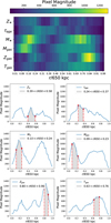 |
Fig. B.1 Upper panel: Stacked saliency map for CNN Model 1, where the baryonic particles of the halo’s central galaxy are divided into 40 uniform radial bins extending from the halo center out to 650 kiloparsecs. These bins are used to construct the input maps for training and testing the model. Lower panel: Line plots showing the pixel intensity variation as a function of normalized radius (r/650) for each row of the stacked saliency map. Each line corresponds to a different physical property. The gray region in each plot indicates the aperture range identified by the network as most relevant for prediction. This region accounts for approximately 22% of the total area under each curve. |
To assess the reliability of the saliency maps in identifying important regions for predicting t1/2, we conducted a series of targeted analyses. We examined first the impact of selecting alternative regions-both around dominant peaks and valleys-from the saliency map profiles of key baryonic properties, say M* in the lower panel of Figure B.1 or Mgas as given in the lower panel of Figure B.2. Retraining the Random Forest model using these regions resulted in only minor variations in predictive performance, suggesting a limited sensitivity to the precise choice of radial interval. We further investigated by computing the Pearson correlation coefficients between the baryonic properties and t1/2 within each bin, focusing on both raw and transformed properties. For CNN Model 2 (with R200c-scaled bins), we observed that while Mgas consistently appeared as the most correlated feature, the overall correlation remained low (typically < 0.35) and relatively flat across bins. Similar trends were noted for CNN Model 1 (fixed 650 kpc binning). These findings suggest that the saliency maps, although somewhat aligned with correlation plots, they are noisy and do not strongly correlate with actual physical trends in the data. As a result, we conclude that while saliency maps can offer a qualitative sense of which features the model considers important, they should be interpreted with caution-particularly because the underlying baryonic properties show weak statistical correlation with t1/2.
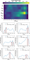 |
Fig. B.2 Upper panel: Stacked saliency map for CNN Model 2, where the halo’s central galaxy baryonic particles are partitioned into 40 uniform bins, ranging from the center of the halo out to 0.3 R200c. These bins are used to construct the input maps for training and testing the model. Lower panel: Line plots showing the pixel intensity variation as a function of normalized radius (r/R200c) for each row of the stacked saliency map. Each line corresponds to a different physical property. The gray region in each plot indicates the aperture range identified by the network as most relevant for prediction. This region accounts for approximately 22% of the total area under each curve. |
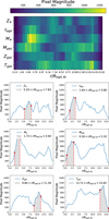 |
Fig. B.3 Upper panel: Stacked saliency map for CNN Model 2, where the halo’s central galaxy baryonic particles are partitioned into 40 uniform bins, ranging from the center of the halo out to 16 Rhalf,fit. These bins are used to construct the input maps for training and testing the model. Lower panel: Line plots showing the pixel intensity variation as a function of normalized radius (r/Rhalf,fit) for each row of the stacked saliency map. Each line corresponds to a different physical property. The gray region in each plot indicates the aperture range identified by the network as most relevant for prediction. This region accounts for approximately 22% of the total area under each curve. |
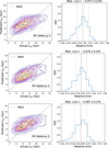 |
Fig. B.4 Comparison of predicted t1/2 values from the three random forest models with their true values from the test dataset. Each model is trained on properties derived from the aperture radial ranges identified by the saliency maps, as listed in Table B.1. Results for the model trained with the aperture range from CNN Model 1 are shown in the first row, CNN Model 2 in the second row, and CNN Model 3 in the third row. Left panel: Two-dimensional joint probability density functions comparing true and predicted t1/2 values. Black points represent predicted versus true values for the random forest model trained on the saliency-identified aperture range. The dotted gray 45-degree line indicates perfect prediction. Right panel: Probability density functions of the relative errors between predicted and true t1/2 values, highlighting the median error and standard deviation. |
References
- Alonso Asensio, I., Dalla Vecchia, C., Bahé, Y. M., Barnes, D. J., & Kay, S. T. 2020, MNRAS, 494, 1859 [CrossRef] [Google Scholar]
- Aloysius, N., & Geetha, M. 2017, in 2017 International Conference on Communication and Signal Processing (ICCSP), IEEE, 0588 [Google Scholar]
- Arendt, A. R., Perrott, Y. C., Contreras-Santos, A., et al. 2024, MNRAS, 530, 20 [Google Scholar]
- Armitage, T. J., Kay, S. T., & Barnes, D. J. 2019, MNRAS, 484, 1526 [NASA ADS] [CrossRef] [Google Scholar]
- Bartalucci, I., Molendi, S., Rasia, E., et al. 2023, A&A, 674, A179 [NASA ADS] [CrossRef] [EDP Sciences] [Google Scholar]
- Bradski, G. 2000, Dr. Dobb’s Journal of Software Tools, 120, 122 [Google Scholar]
- Breiman, L. 2001, Mach. Learn., 45, 5 [Google Scholar]
- Brough, S., Ahad, S. L., Bahé, Y. M., et al. 2024, MNRAS, 528, 771 [NASA ADS] [CrossRef] [Google Scholar]
- Bullock, J. S., Kolatt, T. S., Sigad, Y., et al. 2001, MNRAS, 321, 559 [Google Scholar]
- Burke, C., Hilton, M., & Collins, C. 2015, MNRAS, 449, 2353 [Google Scholar]
- Capalbo, V., De Petris, M., De Luca, F., et al. 2021, MNRAS, 503, 6155 [Google Scholar]
- Chen, Y., Mo, H. J., Li, C., et al. 2020, ApJ, 899, 81 [NASA ADS] [CrossRef] [Google Scholar]
- Chen, X., Zu, Y., Shao, Z., & Shan, H. 2022, MNRAS, 514, 2692 [NASA ADS] [CrossRef] [Google Scholar]
- Chun, K., Shin, J., Smith, R., Ko, J., & Yoo, J. 2023, ApJ, 943, 148 [NASA ADS] [CrossRef] [Google Scholar]
- Contini, E. 2021, Galaxies, 9, 60 [NASA ADS] [CrossRef] [Google Scholar]
- Contini, E., & Gu, Q. 2020, ApJ, 901, 128 [NASA ADS] [CrossRef] [Google Scholar]
- Contini, E., & Gu, Q. 2021, ApJ, 915, 106 [NASA ADS] [CrossRef] [Google Scholar]
- Contini, E., De Lucia, G., Villalobos, A., & Borgani, S. 2014, MNRAS, 437, 3787 [Google Scholar]
- Contini, E., Chen, H., & Gu, Q. 2022, ApJ, 928, 99 [NASA ADS] [CrossRef] [Google Scholar]
- Contini, E., Rhee, J., Han, S., Jeon, S., & Sukyoung, K. Y. 2023, AJ, 167, 7 [Google Scholar]
- Contreras-Santos, A., Knebe, A., Pearce, F., et al. 2022, MNRAS, 511, 2897 [NASA ADS] [CrossRef] [Google Scholar]
- Contreras-Santos, A., Knebe, A., Cui, W., et al. 2023, MNRAS, 522, 1270 [Google Scholar]
- Contreras-Santos, A., Knebe, A., Cui, W., et al. 2024, A&A, 683, A59 [NASA ADS] [CrossRef] [EDP Sciences] [Google Scholar]
- Correa, C. A., Wyithe, J. S. B., Schaye, J., & Duffy, A. R. 2015, MNRAS, 450, 1514 [NASA ADS] [CrossRef] [Google Scholar]
- Croton, D. J., Gao, L., & White, S. D. 2007, MNRAS, 374, 1303 [NASA ADS] [CrossRef] [Google Scholar]
- Cui, W., Murante, G., Monaco, P., et al. 2014, MNRAS, 437, 816 [Google Scholar]
- Cui, W., Power, C., Borgani, S., et al. 2016, MNRAS, 464, 2502 [Google Scholar]
- Cui, W., Knebe, A., Yepes, G., et al. 2018, MNRAS, 480, 2898 [Google Scholar]
- Cui, W., Davé, R., Peacock, J. A., Anglés-Alcázar, D., & Yang, X. 2021, Nat. Astron., 5, 1069 [NASA ADS] [CrossRef] [Google Scholar]
- Cui, W., Dave, R., Knebe, A., et al. 2022, MNRAS, 514, 977 [NASA ADS] [CrossRef] [Google Scholar]
- Cui, W., Jennings, F., Dave, R., Babul, A., & Gozaliasl, G. 2024, MNRAS, 534, 1247 [Google Scholar]
- Darragh-Ford, E., Mantz, A. B., Rasia, E., et al. 2023, MNRAS, 521, 790 [NASA ADS] [CrossRef] [Google Scholar]
- Davé, R., Anglés-Alcázar, D., Narayanan, D., et al. 2019, MNRAS, 486, 2827 [Google Scholar]
- de Andres, D., Cui, W., Ruppin, F., et al. 2022, Nat. Astron., 6, 1325 [NASA ADS] [CrossRef] [Google Scholar]
- de Andres, D., Yepes, G., Sembolini, F., et al. 2023, MNRAS, 518, 111 [Google Scholar]
- de Andres, D., Cui, W., Yepes, G., et al. 2024, MNRAS, 528, 1517 [Google Scholar]
- De Luca, F., De Petris, M., Yepes, G., et al. 2021, MNRAS, 504, 5383 [NASA ADS] [CrossRef] [Google Scholar]
- Desjacques, V., Jeong, D., & Schmidt, F. 2018, Phys. Rep., 733, 1 [Google Scholar]
- Ferragamo, A., de Andres, D., Sbriglio, A., et al. 2023, MNRAS, 520, 4000 [NASA ADS] [CrossRef] [Google Scholar]
- Gao, L., Springel, V., & White, S. D. 2005, MNRAS, 363, L66 [NASA ADS] [CrossRef] [Google Scholar]
- Gianfagna, G., Rasia, E., Cui, W., et al. 2023, MNRAS, 518, 4238 [Google Scholar]
- Golden-Marx, J. B., & Miller, C. J. 2018, ApJ, 860, 2 [NASA ADS] [CrossRef] [Google Scholar]
- Golden-Marx, J. B., & Miller, C. J. 2019, ApJ, 878, 14 [Google Scholar]
- Golden-Marx, J. B., Miller, C., Zhang, Y., et al. 2022, ApJ, 928, 28 [NASA ADS] [CrossRef] [Google Scholar]
- Golden-Marx, J. B., Zhang, Y., Ogando, R., et al. 2025, MNRAS, 538, 622 [Google Scholar]
- Gonzalez, A. H., Zabludoff, A. I., & Zaritsky, D. 2005, ApJ, 618, 195 [Google Scholar]
- Haggar, R., Gray, M. E., Pearce, F. R., et al. 2020, MNRAS, 492, 6074 [NASA ADS] [CrossRef] [Google Scholar]
- Jee, M. 2010, ApJ, 717, 420 [NASA ADS] [CrossRef] [Google Scholar]
- Jiménez-Teja, Y., & Dupke, R. 2016, ApJ, 820, 49 [Google Scholar]
- Jiménez-Teja, Y., Dupke, R., Benitez, N., et al. 2018, ApJ, 857, 79 [Google Scholar]
- Kimmig, L. C., Brough, S., Dolag, K., et al. 2025, A&A, in press, https://doi.org/10.1051/0004-6361/202554777 [Google Scholar]
- Kingma, D. P., & Ba, J. 2014, arXiv e-prints [arXiv:1412.6980] [Google Scholar]
- Klypin, A., Yepes, G., Gottlöber, S., Prada, F., & Hess, S. 2016, MNRAS, 457, 4340 [CrossRef] [Google Scholar]
- Knollmann, S. R., & Knebe, A. 2009, ApJSS, 182, 608 [Google Scholar]
- Kravtsov, A., Vikhlinin, A., & Meshcheryakov, A. 2018, Astron. Lett., 44, 8 [CrossRef] [Google Scholar]
- Krick, J., & Bernstein, R. 2007, AJ, 134, 466 [Google Scholar]
- LeCun, Y., Bottou, L., Bengio, Y., & Haffner, P. 1998, Proc. IEEE, 86, 2278 [Google Scholar]
- LeCun, Y., Bengio, Y., & Hinton, G. 2015, Nature, 521, 436 [Google Scholar]
- Li, Y., Mo, H., & Gao, L. 2008, MNRAS, 389, 1419 [NASA ADS] [CrossRef] [Google Scholar]
- Lim, S., Mo, H., Wang, H., & Yang, X. 2016, MNRAS, 455, 499 [Google Scholar]
- Lin, Y.-T., Mandelbaum, R., Huang, Y.-H., et al. 2016, ApJ, 819, 119 [NASA ADS] [CrossRef] [Google Scholar]
- Lovell, C. C., Wilkins, S. M., Thomas, P. A., et al. 2022, MNRAS, 509, 5046 [Google Scholar]
- Lucie-Smith, L., Barreira, A., & Schmidt, F. 2023, MNRAS, 524, 1746 [NASA ADS] [CrossRef] [Google Scholar]
- Ludlow, A. D., Navarro, J. F., Li, M., et al. 2012, MNRAS, 427, 1322 [NASA ADS] [CrossRef] [Google Scholar]
- Mann, A. W., & Ebeling, H. 2012, MNRAS, 420, 2120 [NASA ADS] [CrossRef] [Google Scholar]
- Matthee, J., Schaye, J., Crain, R. A., et al. 2016, MNRAS, stw2884 [Google Scholar]
- McCarthy, I. G., Schaye, J., Ponman, T. J., et al. 2010, MNRAS, 406, 822 [NASA ADS] [Google Scholar]
- Mihos, J. C., Harding, P., Feldmeier, J., & Morrison, H. 2005, ApJ, 631, L41 [Google Scholar]
- Miyatake, H., More, S., Takada, M., et al. 2016, Phys. Rev. Lett., 116, 041301 [NASA ADS] [CrossRef] [Google Scholar]
- Mo, H., Van den Bosch, F., & White, S. 2010, Galaxy Formation and Evolution (Cambridge University Press) [Google Scholar]
- Molnar, C. 2020, Interpretable machine learning (Lulu.com) [Google Scholar]
- Montes, M., Brough, S., Owers, M. S., & Santucci, G. 2021, ApJ, 910, 45 [Google Scholar]
- More, S., Miyatake, H., Takada, M., et al. 2016, ApJ, 825, 39 [NASA ADS] [CrossRef] [Google Scholar]
- Mostoghiu, R., Knebe, A., Cui, W., et al. 2019, MNRAS, 483, 3390 [NASA ADS] [CrossRef] [Google Scholar]
- Nair, V., & Hinton, G. E. 2010, in Proceedings of the 27th International Conference on Machine Learning (ICML-10), 807 [Google Scholar]
- Navarro, J. F., Frenk, C. S., & White, S. D. 1997, ApJ, 490, 493 [NASA ADS] [CrossRef] [Google Scholar]
- Pedregosa, F., Varoquaux, G., Gramfort, A., et al. 2011, J. Mach. Learn. Res., 12, 2825 [Google Scholar]
- Pillepich, A., Nelson, D., Hernquist, L., et al. 2018, MNRAS, 475, 648 [Google Scholar]
- Planck Collaboration XIII. 2016, A&A, 594, A13 [NASA ADS] [CrossRef] [EDP Sciences] [Google Scholar]
- Power, C., Knebe, A., & Knollmann, S. R. 2012, MNRAS, 419, 1576 [NASA ADS] [CrossRef] [Google Scholar]
- Prada, F., Klypin, A. A., Cuesta, A. J., Betancort-Rijo, J. E., & Primack, J. 2012, MNRAS, 423, 3018 [NASA ADS] [CrossRef] [Google Scholar]
- Presotto, V., Girardi, M., Nonino, M., et al. 2014, A&A, 565, A126 [NASA ADS] [CrossRef] [EDP Sciences] [Google Scholar]
- Ragagnin, A., Andreon, S., & Puddu, E. 2022, A&A, 666, A22 [NASA ADS] [CrossRef] [EDP Sciences] [Google Scholar]
- Rasia, E., Meneghetti, M., & Ettori, S. 2013, Astron. Rev., 8, 40 [Google Scholar]
- Remus, R.-S., Dolag, K., Naab, T., et al. 2017, MNRAS, 464, 3742 [Google Scholar]
- Rudick, C. S., Mihos, J. C., Harding, P., et al. 2010, ApJ, 720, 569 [Google Scholar]
- Santoni, S., De Petris, M., Yepes, G., et al. 2024, A&A, 692, A44 [NASA ADS] [CrossRef] [EDP Sciences] [Google Scholar]
- Shaw, L. D., Weller, J., Ostriker, J. P., & Bode, P. 2006, ApJ, 646, 815 [NASA ADS] [CrossRef] [Google Scholar]
- Simonyan, K., Vedaldi, A., & Zisserman, A. 2013, arXiv e-prints [arXiv:1312.6034] [Google Scholar]
- Srisawat, C., Knebe, A., Pearce, F. R., et al. 2013, MNRAS, 436, 150 [NASA ADS] [CrossRef] [Google Scholar]
- Srivastava, A., Cui, W., Meneghetti, M., et al. 2024, MNRAS, 528, 4451 [Google Scholar]
- Stott, J., Collins, C., Sahlén, M., et al. 2010, ApJ, 718, 23 [Google Scholar]
- Sullivan, J. M., Prijon, T., & Seljak, U. 2023, J. Cosmol. Astropart. Phys., 2023, 004 [CrossRef] [Google Scholar]
- Sunayama, T., & More, S. 2019, MNRAS, 490, 4945 [NASA ADS] [CrossRef] [Google Scholar]
- Tojeiro, R., Eardley, E., Peacock, J. A., et al. 2017, MNRAS, 470, 3720 [NASA ADS] [CrossRef] [Google Scholar]
- Umetsu, K., Zitrin, A., Gruen, D., et al. 2016, ApJ, 821, 116 [Google Scholar]
- Villaescusa-Navarro, F., Anglés-Alcázar, D., Genel, S., et al. 2021, ApJ, 915, 71 [NASA ADS] [CrossRef] [Google Scholar]
- Vitorelli, A. Z., Cypriano, E. S., Makler, M., et al. 2018, MNRAS, 474, 866 [Google Scholar]
- Wadekar, D., Villaescusa-Navarro, F., Ho, S., & Perreault-Levasseur, L. 2020, PNAS, submitted [arXiv:2012.00111] [Google Scholar]
- Wang, L., Weinmann, S. M., De Lucia, G., & Yang, X. 2013, MNRAS, 433, 515 [NASA ADS] [CrossRef] [Google Scholar]
- Wang, K., Mo, H. J., Chen, Y., et al. 2024, MNRAS, 528, 2046 [Google Scholar]
- Watson, D. F., Hearin, A. P., Berlind, A. A., et al. 2015, MNRAS, 446, 651 [NASA ADS] [CrossRef] [Google Scholar]
- Wechsler, R. H., & Tinker, J. L. 2018, ARA&A, 56, 435 [NASA ADS] [CrossRef] [Google Scholar]
- Wechsler, R. H., Bullock, J. S., Primack, J. R., Kravtsov, A. V., & Dekel, A. 2002, ApJ, 568, 52 [NASA ADS] [CrossRef] [Google Scholar]
- Wechsler, R. H., Zentner, A. R., Bullock, J. S., Kravtsov, A. V., & Allgood, B. 2006, ApJ, 652, 71 [NASA ADS] [CrossRef] [Google Scholar]
- White, S. D. M., & Rees, M. J. 1978, MNRAS, 183, 341 [Google Scholar]
- Wong, A. W., & Taylor, J. E. 2012, ApJ, 757, 102 [NASA ADS] [CrossRef] [Google Scholar]
- Yang, X., Mo, H., & van den Bosch, F. C. 2006, ApJ, 638, L55 [CrossRef] [Google Scholar]
- Zehavi, I., Contreras, S., Padilla, N., et al. 2018, ApJ, 853, 84 [NASA ADS] [CrossRef] [Google Scholar]
- Zhang, Y., Yanny, B., Palmese, A., et al. 2019, ApJ, 874, 165 [Google Scholar]
- Zhang, B., Cui, W., Wang, Y., Dave, R., & De Petris, M. 2022, MNRAS, 516, 26 [NASA ADS] [CrossRef] [Google Scholar]
- Zibetti, S., White, S. D., Schneider, D. P., & Brinkmann, J. 2005, MNRAS, 358, 949 [Google Scholar]
- Zu, Y., Mandelbaum, R., Simet, M., Rozo, E., & Rykoff, E. S. 2017, MNRAS, 470, 551 [CrossRef] [Google Scholar]
- Zu, Y., Shan, H., Zhang, J., et al. 2021, MNRAS, 505, 5117 [CrossRef] [Google Scholar]
BCGs refer to the brightest central galaxies or the brightest cluster galaxies.
All linear models are based on a least squares fitting.
All Tables
Halo properties at z = 0 extracted from AHF and utilized within this study to train the RF regressor.
Properties for the BCG and ICL region identified using the 50 h−1 kpc aperture radius for training the RF regressor.
Baryonic properties of the BCG calculated within 30, 50, and 100 h−1 kpc apertures, used to train the RF regressor in this study.
All Figures
|
Fig. 1 Scatter plot depicting the relationship between the logarithmic halo mass at z = 0 and t1/2 in gigayears for the selected sample of halos from The300. The red line represents the best-fit line that has been obtained by fitting a simple linear relation between the halo mass and the t1/2. |
| In the text | |
|
Fig. 2 Upper panel: probability density function of the t1/2 values. Lower panel: histogram for the mass distribution for our selected halos sample used in this study. |
| In the text | |
|
Fig. 3 Left panel: relationship between the true and the predicted t1/2 values using the six trained RF models through a bi-variate joint distribution or 2D probability density function. The black data points represent the scatter between the RF predictions and the true t1/2 values for the test dataset relative to the ideal case of perfect predictions, depicted by a 45-degree dotted gray diagonal line. Right panel: probability density function for the relative errors between the true t1/2 and the predicted values by the RF models, along with the median error and the standard deviation, 1σ. |
| In the text | |
|
Fig. 4 Mean squared error (MSE) for the training, test, and out-of-bag samples for the six models trained using the RF algorithm to assess the model performance. |
| In the text | |
|
Fig. 5 Permutation importance of the features in the six different random forest regressor models we considered in this study. |
| In the text | |
|
Fig. 6 Property maps for a halo with R200c = 1035.84 kpc/h and |
| In the text | |
|
Fig. 7 Architecture of the “single-channel” CNN used in our study. Our network employs two convolutional pooling layers for feature extraction and two fully connected layers for parameter estimation. |
| In the text | |
|
Fig. 8 Predictions of the halo formation time (t1/2) and corresponding accuracy assessment for the three CNN models. Left panel: scatter plots (black points) showing the true versus predicted t1/2 values for the test dataset. Contour lines indicate the joint two-dimensional distribution, and the dashed 45-degree line represents perfect prediction. Right panel: probability density functions of the relative errors between predicted and true t1/2 values, showing the median and standard deviation (1σ) for each model. |
| In the text | |
|
Fig. 9 Correlation between the halo mass M200c and t1/2 across different RF and CNN models. The first and second rows show the correlation trends for the six RF models discussed in Section 3, while the third row corresponds to the three CNN models described in Section 4. In each panel, the shaded red region represents the 16th-84th percentile range of the ML predictions, and the shaded gray region shows the same range for the actual simulation values. The solid red and dotted black lines indicate the median t1/2 in logarithmic mass bins for the ML models and the simulation, respectively. Pearson correlation coefficients are annotated to quantify the strength of the relationship between M200c and the predicted formation times. The solid green line gives the t1/2 - M200c relation based on formation time values calculated using the analytical formalism based on EPS theory as given in Correa et al. (2015). |
| In the text | |
|
Fig. 10 Scatter plot depicting the relation between the concentration parameter cNFW and t1/2 in Gyr for selected sample of halos from The300. The red line depicts the best-fit line obtained by fitting a simple linear relationship between cNFW and t1/2. |
| In the text | |
|
Fig. 11 Correlation between the halo concentration parameter cNFW and t1/2 across different RF and CNN models. The first and second rows show the correlation trends for the six RF models discussed in Section 3, while the third row corresponds to the three CNN models described in Section 4. In each panel, the shaded red region represents the 16th-84th percentile range of the ML predictions, and the shaded gray region shows the same range for the actual simulation values. The solid red and dotted black lines indicate the median t1/2 in logarithmic bins for the ML models and the simulation, respectively. Pearson correlation coefficients are annotated to quantify the strength of the relationship between cNFW and the predicted formation times. |
| In the text | |
|
Fig. 12 The first panel compares the t1/2 predictions with the actual values for the test dataset using a linear model based solely on the magnitude gap M12. The second and third panels show the linear model predictions when additional observable properties from Tables 2 and 3 in Section 2 are incrementally included, namely MBCG/Msat and M14, along with M12. The second panel presents predictions analysis from a linear model using MBCG/Msat along with M12. Similarly, the third panel show predictions analysis based on MBCG/Msat and M14, respectively, combined with M12. In the right column, we show the usual scatter and contour density plots comparing the predicted and actual t1/2s, while the histogram of relative errors is displayed on the right side. We also present the relative error histogram for CNN Model 2, which provides the best balance between median relative error bias (positive median bias) and scatter among the three CNN models. This is for comparing the performance of the linear models with that of the CNN models. |
| In the text | |
|
Fig. A.1 Histograms showing the distribution of 0.3R200c and 16Rhalf,fit for the halos used in this study. In Figure A.1, we show the distributions of 0.3 × R200c and 16 × Rhalf,fit for the halos, representing the maximum edges of the bins used to construct property maps with Binning Methodology 2 and Binning Methodology 3. |
| In the text | |
|
Fig. B.1 Upper panel: Stacked saliency map for CNN Model 1, where the baryonic particles of the halo’s central galaxy are divided into 40 uniform radial bins extending from the halo center out to 650 kiloparsecs. These bins are used to construct the input maps for training and testing the model. Lower panel: Line plots showing the pixel intensity variation as a function of normalized radius (r/650) for each row of the stacked saliency map. Each line corresponds to a different physical property. The gray region in each plot indicates the aperture range identified by the network as most relevant for prediction. This region accounts for approximately 22% of the total area under each curve. |
| In the text | |
|
Fig. B.2 Upper panel: Stacked saliency map for CNN Model 2, where the halo’s central galaxy baryonic particles are partitioned into 40 uniform bins, ranging from the center of the halo out to 0.3 R200c. These bins are used to construct the input maps for training and testing the model. Lower panel: Line plots showing the pixel intensity variation as a function of normalized radius (r/R200c) for each row of the stacked saliency map. Each line corresponds to a different physical property. The gray region in each plot indicates the aperture range identified by the network as most relevant for prediction. This region accounts for approximately 22% of the total area under each curve. |
| In the text | |
|
Fig. B.3 Upper panel: Stacked saliency map for CNN Model 2, where the halo’s central galaxy baryonic particles are partitioned into 40 uniform bins, ranging from the center of the halo out to 16 Rhalf,fit. These bins are used to construct the input maps for training and testing the model. Lower panel: Line plots showing the pixel intensity variation as a function of normalized radius (r/Rhalf,fit) for each row of the stacked saliency map. Each line corresponds to a different physical property. The gray region in each plot indicates the aperture range identified by the network as most relevant for prediction. This region accounts for approximately 22% of the total area under each curve. |
| In the text | |
|
Fig. B.4 Comparison of predicted t1/2 values from the three random forest models with their true values from the test dataset. Each model is trained on properties derived from the aperture radial ranges identified by the saliency maps, as listed in Table B.1. Results for the model trained with the aperture range from CNN Model 1 are shown in the first row, CNN Model 2 in the second row, and CNN Model 3 in the third row. Left panel: Two-dimensional joint probability density functions comparing true and predicted t1/2 values. Black points represent predicted versus true values for the random forest model trained on the saliency-identified aperture range. The dotted gray 45-degree line indicates perfect prediction. Right panel: Probability density functions of the relative errors between predicted and true t1/2 values, highlighting the median error and standard deviation. |
| In the text | |
Current usage metrics show cumulative count of Article Views (full-text article views including HTML views, PDF and ePub downloads, according to the available data) and Abstracts Views on Vision4Press platform.
Data correspond to usage on the plateform after 2015. The current usage metrics is available 48-96 hours after online publication and is updated daily on week days.
Initial download of the metrics may take a while.