| Issue |
A&A
Volume 700, August 2025
|
|
|---|---|---|
| Article Number | A238 | |
| Number of page(s) | 23 | |
| Section | Interstellar and circumstellar matter | |
| DOI | https://doi.org/10.1051/0004-6361/202554316 | |
| Published online | 26 August 2025 | |
Precision analysis of 12C/13C ratios in Orion IRc2 acetylene isotopologs via χ2 fitting
Department of Physics and Origin of Matter and Evolution of Galaxies (OMEG) Institute, Soongsil University,
Seoul
06978,
Republic of Korea
★ Corresponding author.
Received:
28
February
2025
Accepted:
30
June
2025
Abstract
We present a detailed analysis of acetylene (C2H2) and its isotopologs in the Orion IRc2, focusing on the determination of 12C/13C isotopic ratios using high-resolution infrared spectra from SOFIA. By employing a robust χ2 fitting method, we simultaneously determined the temperature and column density, achieving a 12C/13C ratio of 18.73−1.47+1.54 for the blue clump and 15.07−1.60+1.61 for the red clump. These results revealed significant discrepancies with the traditional rotational diagram method, which overestimated the ratios by 12.1% and 23.9%, respectively. Our χ2 approach also reduced uncertainties by up to 75% , providing more precise and reliable isotopic ratios. Additionally, we extended the analysis to isotopologs not covered in HITRAN, calculating vibrational and rotational constants through quantum chemical calculations. This allowed us to model subtle isotopic shifts induced by 13C and deuterium substitution, enabling accurate isotopolog detection in astrophysical environments. The Python package (TOPSEGI) developed in this study facilitates efficient χ2 fitting and isotopic ratio analysis, making it a valuable tool for future high-resolution observations. This work highlights the critical role of advanced spectral models and fitting techniques in understanding isotopic fractionation and the chemical evolution of interstellar matter.
Key words: astrochemistry / line: identification / ISM: abundances / ISM: molecules / infrared: ISM
© The Authors 2025
 Open Access article, published by EDP Sciences, under the terms of the Creative Commons Attribution License (https://creativecommons.org/licenses/by/4.0), which permits unrestricted use, distribution, and reproduction in any medium, provided the original work is properly cited.
This article is published in open access under the Subscribe to Open model. This email address is being protected from spambots. You need JavaScript enabled to view it. to support open access publication.
1 Introduction
The study of ro-vibrational transitions in simple molecules such as acetylene (C2H2)1 and its isotopologs plays a crucial role in understanding the chemical evolution of interstellar environments. Acetylene, a widely observed molecule in planetary atmospheres, interstellar clouds, and carbon-rich stars (see Table 1 (Pentsak et al. 2024), exhibits distinct infrared (IR) spectra that are sensitive to isotope substitution. Among these isotopologs, 13C-substituted acetylene (13CCH2) is of particular interest, as its detection can provide valuable insights into the isotopic composition of interstellar matter and the processes driving galaxy chemical evolution (Jacob et al. 2020).
Carbon, the primary element in acetylene and its isotopologs, is synthesized mainly in intermediate-mass stars (approximately 0.8 M⊙ to 8 M⊙) through thermonuclear fusion reactions (Karakas 2010). The dominant product of the triple-alpha process is 12C, while 13C is produced over longer timescales as a secondary product of stellar nucleosynthesis. In asymptotic giant branch (AGB) stars, 13C is primarily formed as a byproduct of the CNO cycle. This process begins with the fusion of 12C and protons, resulting in 13N, which subsequently decays via positron emission into 13C (Pagel 2009). Once formed, carbon combines into simple carbon-bearing molecules such as acetylene (C2 H2), CO, and HCN within stellar atmospheres (McCarthy et al. 2019). These molecules are then dispersed into the interstellar medium (ISM) by stellar winds, enabling the formation of additional carbon compounds. The widespread distribution of these carbon-bearing molecules across the Universe provides a unique opportunity to trace stellar nucleosynthesis processes and the chemical evolution of interstellar environments.
The 12C/13C ratio, determined through the study of carbon-bearing molecules such as acetylene (C2H2), serves as an essential diagnostic tool for tracing the history of nucleosynthesis and the chemical evolution of galaxies. In the Solar System, this ratio is approximately 80 (Woods 2010), whereas in carbon stars such as Y CVn, it has been observed to be as low as 3.5 (Lambert et al. 1986), indicating a significant enhancement of 13C in certain astrophysical environments. These variations in isotopic ratios offer crucial insights into processes such as stellar nucleosynthesis, mass loss in evolved stars, and the chemical enrichment of the ISM. By analyzing ro-vibrational spectra of molecules such as acetylene, precise isotopic ratios can be derived, enabling a deeper understanding of the chemical and physical conditions within diverse astrophysical environments.
Among various carbon-bearing molecules, acetylene (C2H2) and its isotopologs offer a particularly effective means for probing 12C/13C ratios in interstellar environments. Infrared spectroscopy of acetylene enables the precise estimation of molecular column densities (N) by leveraging rotational quantum numbers (J) and total internal partition sums (TIPS) under the assumption of local thermodynamic equilibrium (LTE). These molecular abundances, when combined with isotopolog-specific spectra, provide valuable information on the chemical and physical conditions of interstellar clouds and star-forming regions. However, traditional analysis methods, such as the rotational diagram (RD) method (Goldsmith & Langer 1999), often overestimate 12C/13C ratios due to their reliance on linear extrapolations and the separate fitting of temperature (T) and column density. These limitations introduce systematic biases and reduce the reliability of the derived isotopic ratios, highlighting the need for more robust and accurate fitting approaches.
To overcome the limitations of traditional methods, we implemented the χ2 fitting approach to analyze the Orion IRc2, a chemically diverse and dynamically intricate site of massive star formation within the Becklin-Neugebauer/Kleinmann-Low (BN/KL) region of the Orion molecular cloud (OMC-1). This area, illustrated in Fig. 1, features bright stars embedded within dense interstellar clouds illuminated by cosmic dust. Such a complex and rich environment provides an ideal setting for studying isotopic fractionation processes and their role in the chemical evolution of interstellar matter (Stahler & Palla 2008). Specifically, our analysis targeted the kinematic components of the IRc2, referred to as the blue and red clumps, which exhibit distinct line-of-sight velocities and unique molecular compositions. The line-of-sight velocities, as measured by Nickerson et al. (2023), are vLSR = −7.1 ± 0.7 km s−1 for the blue clump and vLSR = 1.4 ± 0.5 km s−1 for the red clump. The high spectral resolution and dynamic range of this region make it particularly suitable for evaluating the accuracy and advantages of the χ2 method in isotopic ratio determinations.
Using high-resolution infrared spectra from SOFIA/EXES, the χ2 fitting method determines the temperature (T) and the column density (N) simultaneously by minimizing residuals between observed and theoretical lower-state column densities. Compared to the RD method, the χ2 approach reduced the uncertainties by up to 75% in the blue clump and corrected RD overestimations of the 12C/13C ratios by 12.1% and 23.9% for the blue and red clumps, respectively. These results underscore the utility of such advanced techniques as the χ2 method in probing isotopic and chemical properties of massive star-forming regions. Furthermore, the spatial and kinematic separation of the blue and red clumps reveals their distinct physical origins and evolutionary processes within the BN/KL complex.
To improve the efficiency and broaden the scope of our analysis, we incorporated a QuadTree search algorithm into the χ2 fitting method, enabling targeted exploration of the parameter space and minimizing computational overhead. Furthermore, we extended our study to all isotopologs of acetylene substituted with 13 C and deuterium (D), calculating their rotational and vibrational constants using quantum chemical methods such as the density functional theory (DFT) and Møller-Plesset perturbation theory (MP2). These calculations filled critical gaps in existing data, particularly for isotopologs absent in HITRAN (High-Resolution Transmission Molecular Absorption database) (Jacquemart et al. 2003; Gordon et al. 2022), and revealed significant isotopic effects, including shifts in vibrational modes caused by 13C and D substitutions.
By combining advanced computational techniques with high-resolution observations, our approach offers a robust framework for precise isotopic ratio determinations. The Python package developed in this study further strengthens this framework by automating the analysis and enabling direct comparisons between the RD and χ2 methods. This tool simplifies isotopic ratio calculations, facilitating future research into isotopic fractionation, molecular abundances, and the chemical evolution of diverse astrophysical environments with greater precision and reduced biases.
The structure of this paper is as follows. Section 2 provides an overview of the observational data, including previous spectral analyses of acetylene and its isotopologs such as 13 CCH2 and C2HD. Section 3 presents the findings of our reanalysis in three parts: Sect. 3.1 focuses on the results for C2H2, 13 CCH2, and C2 HD; Sect. 3.2 discusses theoretical calculations for seven isotopologs absent from the HITRAN database; and Sect. 3.3 compares the 12C/13C isotopic ratios derived using the RD and χ2 methods, summarizing the differences and improvements. Finally, in Sect. 4 we conclude the paper by highlighting the implications of these findings, particularly the advantages of the χ2 fitting method for isotopic studies in astrophysical environments.
Details of the quantum chemical tools used, including Gaus-sian16 and DFT calculations, are summarized in the appendix. The appendix also provides precomputed spectral data, instructions for using the Python package developed in this study, and guidance on accessing the code via GitHub. This package enables automation of the fitting process, offering a direct comparison between RD and χ2 methods while filling critical gaps in existing datasets, thereby supporting future research in isotopic ratio determinations.
Occurrence of acetylene in various astrophysical environments and objects.
 |
Fig. 1 Location of Orion IRc2 within the BN/KL region of OMC-1, marked by the black circle (Fernique et al. 2015). |
Normal vibrational modes of C2H2 (Chubb 2018).
2 Observations
2.1 A brief introduction to acetylene and its isotopologs
Acetylene is a simple organic molecule widely observed in various astrophysical environments. Its lack of a permanent dipole moment prevents it from producing detectable rotational spectra in the radio range, but it is identified through ro-vibrational transitions in the mid-infrared region. Acetylene exhibits seven normal vibrational modes, characterized by symmetric and antisymmetric stretching and bending motions. Among these, the symmetric and anti-symmetric bending modes (ν4, ν5) are doubly degenerate, reducing the number of distinct modes to five (McQuarrie 2008).
As summarized in Table 2, the ν3 (CH anti-symmetric stretch) and ν5 (anti-symmetric bend) modes are infrared active, while the ν1 (CH symmetric stretch), ν2 (CC symmetric stretch), and ν4 (symmetric bending) modes are infrared inactive due to their symmetry. The degeneracy of ν4 and ν5 plays a critical role in shaping the vibrational spectra of acetylene, especially when analyzing its isotopologs. This classification highlights how distinct vibrational modes contribute to the molecule’s overall spectral characteristics.
For symmetric isotopologs of acetylene, such as C2H2, C2D2, and 13C2H2, two nuclear spin isomers – ortho and para – are present, introducing additional complexity to the spectral analysis (Herman & Lievin 1982). The ortho isomer corresponds to parallel nuclear spins, while the para isomer has antiparallel spins, resulting in distinct population distributions among rotational energy levels. These spin isomers significantly influence the ro-vibrational spectra, facilitating the identification of acetylene isotopologs in diverse astrophysical environments. This, in turn, enhances our understanding of molecular abundances and isotopic ratios, which are critical for studying the chemical evolution of interstellar regions (Herman 2007).
The diverse detection of acetylene across astrophysical environments builds on this spectral complexity, showcasing its utility as a molecular tracer for interstellar chemistry. Infrared spectra of acetylene have been observed on various planets, including Jupiter, Saturn, Uranus, and Neptune, through techniques such as mid-infrared spectroscopy with Cassini/CIRS (Nixon et al. 2007) and Voyager 2/IRIS (Bézard et al. 1991). Beyond planetary atmospheres, acetylene has been identified in the atmosphere of Titan (Bézard et al. 2022), the comet Hyakutake (Brooke et al. 1996), and carbon-rich environments such as IRC +10216 (Fonfría et al. 2008) and the Orion Molecular Cloud IRc2 (Rangwala et al. 2018). These findings illustrate how acetylene serves as a valuable diagnostic tool, tracing the processes that shape the chemical evolution of stellar and planetary systems across a range of environments and stages of formation.
Understanding and interpreting these observations require reliable molecular spectroscopic databases, such as ExoMol (Tennyson et al. 2024) and HITRAN (Gordon et al. 2022). The ExoMol project aims to comprehensively cover the spectroscopic properties of molecules relevant to hot astrophysical environments. For example, CO appears in the stellar spectra and requires spectroscopic data at temperatures above 6000 K (Tennyson et al. 2016). Among its outputs, the aCeTY line list, developed as a part of the ExoMol project, provides ro-vibrational transition data for C2H2 (Chubb et al. 2018, 2020). In contrast, the HITRAN database has been primarily developed for terrestrial and planetary atmospheres and offers line lists not only for C2H2 but also for its isotopologs such as 13CCH2 and C2HD. Since this study involves acetylene isotopologs such as 13CCH2 and was performed under relatively low-temperature conditions (approximately 50–300K), we adopted the HITRAN database.
2.2 SOFIA observational data
Infrared observational data for acetylene and its isotopologs have been obtained using various instruments, including the Spitzer Space Telescope and the SOFIA observatory. Among these, SOFIA provides superior spectral resolution, enabling the precise resolution of individual rotational transitions that are critical for accurately determining molecular column densities (Rangwala et al. 2018; Nickerson et al. 2023). This advantage makes SOFIA particularly well-suited for studies requiring high-resolution spectroscopic data, such as the analysis of isotopic ratios in chemically complex regions. In this study, we specifically use SOFIA observations to validate and refine our proposed methodology for isotopic ratio determination.
The mid-infrared data from SOFIA used in this study focuses on the IRc2 near the Orion Nebula (M42 or NGC 1976), a well-known gas cloud illuminated by radiation from the Trapezium stars. Although it is neither the largest nor the brightest H II region, the Orion Nebula is one of the closest and most thoroughly studied star-forming regions (O’Dell 2001). Approximately 0.2 pc behind the nebula are the Becklin-Neugebauer (BN) and IRc2 infrared sources, located within the Kleinman–Low (KL) nebula (Stahler & Palla 2008). The Orion BN-KL region represents one of the nearest and most extensively investigated sites of massive star formation. While much of the region’s chemistry has been explored at radio, (sub)mm, and far-infrared (FIR) wavelengths, mid-infrared (MIR) spectroscopic observations, such as those of the IRc2, offer unique insights into its chemical composition, kinematics, geometry, and physical conditions (Nickerson et al. 2023). This makes SOFIA’s MIR data invaluable for probing the complex environments of massive star formation.
2.3 Spectral analysis of C2H2 and 13CCH2
In molecular spectroscopy, rotational transitions are classified into three branches based on changes in the rotational quantum number J: the P-branch (∆J = −1), Q-branch (∆J = 0), and R-branch (∆J = +1). These transitions are fundamental to ro-vibrational spectra, revealing essential details about molecular energy states. SOFIA’s mid-infrared observations encompass all three branches, enabling a comprehensive analysis of acetylene and its isotopologs.
For acetylene (C2H2) and its isotopolog 13CCH2, ro-vibrational transitions in the mid-infrared region, particularly around the ν5 band, allow detailed analysis of molecular properties.
Figure 2 illustrates the observed spectra of C2H2 and 13CCH2, corrected for Doppler shifts and Local Standard of Rest (LSR) velocities to ensure precise alignment with theoretical predictions from the HITRAN database. The black line represents the observed data for the Orion IRc2, while the blue and green lines correspond to the predicted transitions for C2H2 and 13CCH2, respectively. The dashed lines indicate Doppler corrections, and the dash-dotted lines represent adjustments for both Doppler and LSR corrections, essential for accurately determining molecular column densities, excitation conditions, and velocity structures. Without these corrections, the spectral lines would appear shifted, leading to systematic errors. The LSR correction further ensures that the observed spectra are referenced to the standard rest frame of the interstellar medium, providing more accurate velocity measurements.
The six panels in Fig. 2 – three middle and three lower panels – provide a comprehensive view of the ro-vibrational transitions for both ortho and para species of C2H2, along with the isotopolog 13CCH2. The upper panel displays a broader spectral range, highlighting multiple ro-vibrational transitions across the P-, Q-, and R-branches. The three middle panels focus on individual transitions of C2H2, specifically the J = 10 → 9, J = 11 → 10, and J = 12 → 11 transitions, with the blue vertical solid lines denoting HITRAN predictions. The three lower panels present detailed views of 13CCH2 transitions at J = 10 → 9, J = 11 → 10, and J = 13 → 12, marked by green vertical solid lines corresponding to HITRAN predictions.
The excellent agreement between HITRAN predictions and SOFIA observations across all panels confirms the reliability of the applied corrections and the accuracy of the spectral models. These high-resolution spectra allow for precise evaluation of physical conditions within the Orion hot core, such as temperature, column density, and velocity structure, which are critical for understanding the chemical processes driving the evolution of this massive star-forming region.
3 Results
This section presents the application of the χ2 fitting method for deriving temperature (T) and column density (N) from observational data. By simultaneously fitting N and T, the method provides consistent results for the ortho and para species of C2H2, as well as 13CCH2. Additionally, theoretical predictions are made for C2HD and other isotopologs not included in the HITRAN database, offering a framework for future studies on these species.
3.1 C2H2, 13CCH2, and C2HD
3.1.1 IR spectroscopy
The HITRAN database provides detailed spectral line parameters for C2H2 and its isotopologs, 13CCH2 and C2HD, including transition frequencies, line intensities, and broadening coefficients. In the P, Q, and R branches of these species, each transition corresponds to a specific ro-vibrational energy change, which can be directly compared with experimental data or used for modeling. For 13CCH2, the substitution of 12C with 13C results in small spectral line shifts due to the slight increase in mass affecting the rotational constants. In C2HD, the substitution of hydrogen (H) with deuterium (D) causes significantly larger shifts, reflecting the substantial mass difference between hydrogen and deuterium. These isotopic shifts provide valuable information for distinguishing isotopologs in high-resolution spectroscopic analyses. These precise line positions and intensities are crucial for high-resolution spectroscopy, enabling accurate analyses of molecular clouds and planetary atmospheres in astrophysical studies. Instruments such as SOFIA/EXES rely on such data for direct comparisons with observed spectra, facilitating detailed investigations of molecular environments.
Table 3 presents the ν5 vibrational mode frequencies and the rotational constants (B̃) for C2H2 and its isotopologs, 13CCH2 and C2HD, along with the frequency scale factor (FSF) values derived from HITRAN data. The FSF values demonstrate consistent scaling across all isotopologs, ensuring the reliability of the vibrational and rotational parameter predictions. For C2H2, serving as the reference molecule, our calculated and rescaled ν5 frequency of 729.185 cm−1 (with FSF=0.941337) and rotational constant B̃ of 1.1766 cm 1 are in excellent agreement with previously published results (729.08 cm−1 and 1.1766 cm−1) (El Idrissi et al. 1999; Herman 2007). Similarly, for 13CCH2, the ν5 frequency of 728.252 cm−1 (with FSF=0.941522) and B̃ value of 1.1485 cm−1 are also in excellent agreement with the findings of Fayt et al. (2007) (728.27 cm−1 and 1.1485 cm−1). In the case of C2HD, our calculations yield a ν5 frequency of 677.856 cm−1 with FSF=0.972094, and a B̃ value of 0.9901 cm−1, which are highly consistent with the results reported by Herman et al. (2004) and Wlodarczak et al. (1989) (676.09 cm−1 and 0.9915 cm−1).
In this study, the B3LYP DFT method was employed for all quantum chemical calculations (Becke 1988; Lee et al. 1988). This choice was made after comparing various quantum chemical methods, including HF, B3LYP, PBE0, and MP2, where B3LYP demonstrated the highest accuracy in reproducing known experimental spectra. Consequently, unless otherwise stated, all quantum chemical results presented in this work, including vibrational and rotational parameters, were calculated using the B3LYP method. For further details on the performance and results of other quantum chemical methods, please refer to Appendices B and C.
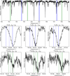 |
Fig. 2 Mid-infrared spectra of IRc2 near the Orion Nebula (M42 or NGC 1976). Upper panel: SOFIA observational data (black lines). Middle panel: C2H2 absorption lines corresponding to R-branch. Lower panel: 13CCH2 absorption lines corresponding to R-branch. Vertical lines correspond to the HITRAN database (solid), the LSR corrections (dashed), and corrections for both the LSR and Doppler effects (dash-dotted). The shading around the dash-dotted lines represents the error associated with the transformation to the LSR. |
Comparison of normal modes and rotational constants of various isotopologs of C2H2 between this work (B3LYP) and related studies.
3.1.1 Extraction of T and N from χ2 method
Under LTE, the population of lower energy states (Nl) is expressed as (Goldsmith & Langer 1999)
 (1)
(1)
where Q is the partition function (or TIPS) (Gamache et al. 1990; Fischer et al. 2003; Amyay et al. 2011; Laraia et al. 2011), and El and gl represent the energy and degeneracy of the lower state, respectively. By taking the natural logarithm, this expression can be transformed into a linear equation:
 (2)
(2)
which forms the basis of the traditional RD method. In this method, ln(Nl/gl) and El/kB are used as y and x coordinates, respectively, to perform a linear fit. While this approach allows for the estimation of temperature (T) from the slope and column density (N) from the intercept, it assumes that T and N are independent, neglecting the dependence of the partition function Q on T.
To overcome this limitation, the χ2 method is introduced, treating T and N as two variables to be optimized simultaneously. The theoretical values  are computed based on T and N, and the differences from the observed values
  are minimized using
 (3)
(3)
where σobs accounts for observational uncertainties. By finding the T and N values that minimize χ2, the method provides a more robust and accurate estimation of physical parameters.
The analysis of acetylene (C2H2) and its isotopolog 13CCH2 was conducted for two distinct velocity components, referred to as the blue clump and red clump. These components are characterized by their unique velocity shifts and allow for the assessment of the physical conditions of the molecular gas. In this section, we focus on the blue clump, which is distinguished by its relatively narrow velocity dispersion and prominent ro-vibrational features.
Figure 3 presents the analysis of the blue clump component for acetylene (C2H2) and its isotopolog 13CCH2 using two methods: the traditional RD method and the newly implemented χ2 fitting method for the blue clump component. The left panels display log10(Nl/gl) as a function of the lower rotational quantum number Jl, derived from SOFIA high-resolution observations, with data from Nickerson et al. (2023). Transitions in the P-, Q-, and R-branches are represented by purple triangles, yellow rectangles, and blue circles, respectively, with 1σ error bars included for each point. The blue shaded regions indicate the uncertainty range associated with the RD method, while the blue solid line represents the best-fit result obtained through linear fitting. In contrast, the red line shows the best-fit result derived from the χ2 method, demonstrating greater accuracy and reliability.
The right panels illustrate the confidence intervals for the χ2 method with two degrees of freedom, temperature (T) and column density (N). These plots visualize the agreement between the observed and theoretical lower-state column densities (Nl). The minimum contour value marks the best-fit parameters, with red stars indicating the results from the χ2 method and blue stars representing those from the RD method. The associated error bars for the RD method are also shown. The best-fit values of T and N are explicitly stated in red text in the lower-left corner of each panel. This analysis demonstrates the effectiveness of the χ2 method in interpreting complex molecular spectra. Compared to the RD approach, the χ2 method achieves a significantly lower χ2 value, highlighting its superior reliability in determining the physical conditions within the blue clump.
Figure 4 extends the analysis to the red clump component for acetylene (C2H2) and its isotopolog 13CCH2, following the same methodology as used for the blue clump. The red clump represents another distinct velocity component, enabling a complementary investigation of its physical properties.
The analysis of the red and blue clumps reveals distinct differences in parameter uncertainties and fitting performance between the χ2 and RD methods. For the blue clump, the χ2 method demonstrates a significant improvement by reducing error bars by up to 75% compared to the RD method. This reduction highlights the robustness and precision of the χ2 approach, which simultaneously fits temperature (T) and column density (N) while accounting for statistical weights and degeneracy factors. The improved precision underscores the advantage of global fitting over linear extrapolation in traditional RD methods, particularly for symmetric molecules such as C2H2 . In contrast, the red clump shows larger uncertainties for 13CCH2 when using the χ2 method compared to the RD method. This is evident in the left panel of Fig. 4, where the red band (representing the uncertainty range from the χ2 method) is noticeably broader than the blue band (uncertainty range from the RD method). The increase in uncertainty arises from the limited number of observational data points (four) used in the fitting process. In the χ2 fitting method, the uncertainty in the parameters is inversely proportional to the square root of the degrees of freedom, calculated as Ndata - Nparameters. With only four data points and two fitting parameters (T and N), the degrees of freedom are minimal (2), leading to inherently larger uncertainties in the χ2 fitting compared to cases with higher observational coverage. This highlights the critical role of sufficient data points to achieve reduced uncertainties in multi-parameter fitting methods.
Despite the larger uncertainties observed in the χ2 method for the red clump, it is notable that the center values of 13CCH2 derived from both the RD and χ2 methods are remarkably similar.
These findings underscore the complementary nature of the RD and χ2 methods. While the RD method provides a quick estimation with smaller uncertainties in cases of sparse data, the χ2 method offers a more detailed and statistically consistent analysis, making it particularly valuable for datasets with higher observational coverage. Moving forward, improving data quality and quantity will be crucial to fully leverage the precision and reliability of advanced fitting methods such as χ2 in astrophysical studies.
Figure 5 compares the calculated log10(Nl/gl) values for C2HD as a function of the lower rotational quantum number Jl at four temperatures (T = 100 (solid), 300 (dashed), 500 (dotted), and 1000 (dot-dashed) K). The red lines represent the results using the TIP function calculated in this work, while the blue lines correspond to reference values based on the HITRAN TIP function.
The results show excellent agreement across the full range of Jl, especially at higher temperatures (T = 500 K and 1000 K), where deviations are negligible. Slight discrepancies at lower temperatures (T = 100 K and 300 K) for higher Jl values likely arise from differences in partition function calculations. However, these deviations remain well within acceptable limits, confirming the accuracy and robustness of the TIP function derived in this study. This comparison highlights the reliability of the proposed approach for spectroscopic studies and its consistency with established databases such as HITRAN. For a detailed discussion on the TIP function and its calculations, refer to Sect. 3.2.1.
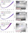 |
Fig. 3 Analysis of the ν5 band of C2H2 and 13CCH2 using the RD and the χ2 fitting methods. Left panels: plot of log10 (Nl/gl) as a function of the lower rotational quantum number Jl, Right panels: contour plots from the χ2 method. In the left panels, purple triangles, yellow rectangles, and blue circles indicate observational results for the P-, Q-, and R-branches, respectively, based on the Nickerson et al. (2023) study of Orion IRc2. Each point includes 1σ error bars. The blue shaded regions represent the 1σ uncertainty range for the RD method, with the blue solid line showing the best-fit result. The red line represents results from the χ2 method, providing more precise estimates of physical parameters. The right panels display contour plots illustrating the confidence intervals for the χ2 method with two degrees of freedom, temperature (K) and column density (molecules per square centimeter). The contours depict the difference between observed and theoretical lower-state column densities (Nl), with the minimum value indicating the best-fit parameters. The red star marks the best-fit temperature and column density from the χ2 method, while blue stars with error bars denote the RD best-fit values with 1σ uncertainties. Contour levels correspond to confidence levels, and the explicit best-fit values of T and N are displayed in red in the lower-left corner. These results emphasize the improved accuracy of the χ2 fitting method (right panels) compared to the RD approach (left panels) in determining the physical properties of the blue clump component. Additionally, the X-shaped hatching in the right panels indicates regions where ∆χ2 is too large, making numerical calculations infeasible. |
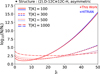 |
Fig. 5 Comparison of calculated log10(Nl/gl) values for C2HD as a function of the lower rotational quantum number Jl at different temperatures (T = 100 (solid), 300 (dashed), 500 (dotted), and 1000 (dot-dashed) K). The red lines represent the values using our calculated TIP function, while the blue lines correspond to the reference results using the HITRAN TIP function. The agreement between this work and HITRAN validates the accuracy of the current method, particularly at higher temperatures, where deviations are minimal. |
3.2 The remaining isotopologs of acetylene not mentioned in HITRAN
HITRAN is widely trusted in the field due to its comprehensive and accurate data, which is crucial for spectroscopic analyses. However, for acetylene, HITRAN provides only three types of TIPS (Gamache et al. 2021), which limits the data available for isotopolog studies. To overcome this, we performed additional quantum chemical calculations using Gaussian16 for a total of seven acetylene isotopes (excluding the two in the previous section), 13C2H2, D12C13CH, D13C12CH, C2D2, 13C2HD, 13CCD2, and 13C2D2) using four different quantum chemistry methods: HF, DFT with B3LYP and PBE0, and MP2. For quantum chemical calculation methodology, see Appendix B; for fundamental frequencies corresponding to ν1 ~ ν5 and detailed calculation results and discussion, see Appendix C.
3.2.1 Total internal partition sum
The TIPS of a molecule represents the sum of contributions from all possible energy states and is crucial for accurately modeling molecular properties across a range of temperatures. It can be calculated as
 (4)
(4)
where ϵ represents the energy levels. These levels are typically decomposed into rotational and vibrational components2:
 (5)
(5)
Using these separated energy levels, the total partition function is expressed as
 (6)
(6)
For linear molecules such as acetylene, the rotational energy form can be expressed as follows:
 (7)
(7)
where B̃ is the rotation constant expressed in inverse centimeters,
 (8)
(8)
and D̃J is the centrifugal distortion constant.
The rotational constants (B̃) for each isotopolog of acetylene were determined using quantum chemical calculations based on the B3LYP method. For C2H2, 13CCH2, and C2HD, the FSF values for ν5 and D̃J were optimized to match the observed spectra from HITRAN. For the remaining isotopologs, FSFs were estimated based on structural similarities. Table 4 summarizes the FSF, B̃, and D̃J values used for acetylene and its isotopologs in this study.
To validate the reliability of the computed ν5 and B̃ values, we compared them against experimental data for the minor isotopologs (IDs 3–9) that are not included in HITRAN. The experimental ν5 band centers were obtained directly from rovibrational spectra, whereas the rotational constants B̃ were derived through fitting of the observed transition lines. A detailed comparison is presented in Appendix E (Table E.1), which shows that our calculated values agree with experimental results within 0.3% for ν5 and 0.5% for B̃. These results support the accuracy of our quantum chemical methodology. The experimental values were compiled from high-resolution spectroscopic studies (Tamassia et al. 2016; Predoi-Cross et al. 2012; Fusina et al. 2011; Huet et al. 1991; Fusina et al. 2014; Canè et al. 2002).
The centrifugal distortion term (D̃J) plays a more significant role at large values of J, opposing the leading rotational constant term and introducing potential deviations in the calculated energy levels. While higher-order correction terms are necessary to fully account for these effects, they are omitted in this study to prioritize computational efficiency and focus on primary contributions. This simplification may explain discrepancies observed at high J values, especially for isotopologs with pronounced centrifugal distortion effects.
With this energy spectrum, the rotational partition function is calculated as follows:
 (9)
(9)
where the gJ = (2J + 1) is the degeneracy factor of the given energy ϵJ. The gi describe the state-independet degeneracy factor. For acetylene, we use the “astronomer convention” in which para:ortho species ratio is 1/4:3/4, resulting in  . In contrast, the “atmospheric convention” assumes a para:ortho ratio of 1:3, yielding
  . Thus, the
  value in the atmospheric convention is 4 times larger than in the astronomer convention (
 ). For all other molecules, the atmospheric convention was used. Therefore, when using other conventions, such as the astronomer convention, it is suggested to multiply by an appropriate constant.
The vibrational energy levels are given by
 (10)
(10)
where vq is the vibrational quantum number.
The ν represents the vibrational frequency of the molecules,
 (11)
(11)
where the k is the spring constant of the molecule and μ is the reduced mass of the same molecule. The ν̄ ≡ (ν/c) is the wave number in inverse centimeters.
The vibrational partition function of a linear molecule is
 (12)
(12)
Table 5 summarizes the properties of various isotopologs of acetylene, including isotopolog ID, isotopical name, nuclear spin values for each atom (I (C1 + H1) and I(C2 + H2)), total degeneracy, symmetry statistics (Fermi or Bose), rovibronic and nuclear spin wavefunctions (Ψrov × Ψns = Ψtot), J parity (even or odd), and statistical weights (gi). The total degeneracy is calculated using the formula (2I(C1 + H1) + 1)(2I(C2 + H2) + 1), which accounts for the contributions of nuclear spin states for the relevant nuclei. For symmetric isotopologs such as C2H2, 13C2 H2, C2D2 and 13C2 D2 (Herman et al. 2003), specific symmetry constraints result in distinct statistical weights for even and odd J states, following Fermi-Dirac or Bose–Einstein statistics. In contrast, asymmetric isotopologs, such as H13C12CH (13CCH2), C2HD, D12C13CH, D13C12CH, D13C13CH (13C2HD), D13C12CD (13CCD2), exhibit altered nuclear spin configurations that lead to higher degeneracies and statistical weights due to the larger number of possible spin states. These gi factors are critical for calculating molecular partition functions, understanding the relative populations of ro-vibrational states, and accurately modeling molecular spectra.
Figure 6 presents a comparison of the total internal partition sums (Qtot) as a function of temperature for acetylene (C2H2), 13 CCH2, and C2HD. The solid blue lines represent the partition sums calculated in this work, while the red dashed lines correspond to the values provided by HITRAN. Across the temperature range of 0–1000 K, our results show excellent agreement with the HITRAN data, confirming the reliability of our method for calculating partition sums. The slight deviations at higher temperatures, particularly for 13CCH2, can be attributed to the different computational approaches used. Overall, these comparisons validate the robustness of our approach in predicting partition sums for acetylene isotopologs, ensuring accurate results for future spectral analysis. The slight deviations at higher temperatures, particularly for 13CCH2, can be attributed to the different computational approaches used. Overall, these comparisons validate the robustness of our approach in predicting partition sums for acetylene isotopologs, ensuring accurate results for future spectral analysis. For TIP results for the remaining seven isotopoloues of acetylene, see Appendix D.
Rotational constants (B̃) and centrifugal distortion constants (D̃J) for acetylene (C2H2) and its isotopologs, determined using quantum chemical calculations based on the B3LYP method.
Statistical weights of acetylene isotopologs.
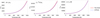 |
Fig. 6 Comparison of the total internal partition sums (Qtot) as a function of temperature for acetylene (C2H2), 13 CCH2, and C2HD. The solid blue line represents the results from this work, while the red dashed line shows the HITRAN values. The agreement between our calculations and HITRAN demonstrates the accuracy of our method across a wide temperature range (0–1000 K). |
3.2.2 χ2 methods for the remaining acetylene isotopolog
Here, we consider 13C2H2 (Isotopolog “3” in our convention) as a specific example to evaluate the performance of our two-parameter fitting method using chi-squared (χ2) calculations. In the absence of actual observational data, we generated a pseudo dataset to demonstrate how the method can be applied to isotopologs with unique statistical properties. This analysis highlights the versatility of our approach in determining temperature and column density, and provides a framework for studying astrophysical environments such as carbon-rich stars or regions with high 13C abundance.
Figure 7 shows the results for 13C2H2, focusing on the estimation of temperature (T) and column density (N). The first and second panels from the top present log10(Nl/gl) as a function of the lower rotational quantum number Jl, with purple triangles, yellow rectangles, and blue circles representing P-, Q-, and R-branch transitions, respectively. The blue shaded regions indicate the 1σ uncertainty from the RD method, while the blue solid line denotes the best-fit result using this method. The red line corresponds to the best-fit result derived from our two-parameter fitting method, demonstrating the improved accuracy and flexibility of the latter. The third and fourth panels from the top illustrate the confidence intervals for the χ2 method with two degrees of freedom, temperature (T) and column density (N). The right panels display contour plots illustrating the confidence intervals for the χ2 method with two degrees of freedom, T and N. Darker regions represent higher ∆χ2 values, while lighter regions correspond to the lower ∆χ2, which provides the best estimates for T and N. Unlike the C2H2 (Isotopolog “0”), 13 C2 H2 (Isotopolog “3”) has a flipped statistical weight due to its nuclear spins and Boson statistics, where even rotational states have a larger weight than odd states. This is reflected in the distinct separation of fitting results for even and odd rotational states, highlighting the molecule’s unique symmetry properties.
Figures 8 and 9 show the predicted log10(Nl/gl) values for the remaining isotopologs of acetylene, based on quantum chemical calculations. (Figure 8 presents results for 13C2H2 (Isotopolog “3”), D12C13CH (Isotopolog “4”), D13C12CH (Isotopolog “5”), and C2D2 (Isotopolog “6”). Figure 9 extends the analysis to 13C2HD (Isotopolog “7”), 13CCD2 (Isotopolog “8”), and 13C2D2 (Isotopolog “9”). For symmetric molecules (13C2H2, 12C2D2, and 13C2D2), even Jl states start at Jl = 0, while odd Jl states begin at Jl = 1, reflecting their symmetry constraints. Asymmetric molecules, such as D12C13CH and D13 C12CH, exhibit continuous distributions across Jl. Each panel illustrates how the population distributions vary under different temperatures, providing insights into the statistical and symmetry properties of these isotopologs. These results serve as a theoretical reference for identifying and characterizing acetylene isotopologs in various astrophysical environments. See Appendix F for the line lists used to generate Figs. 8 and 9.
3.3 Comparison of results and the 12C/13C column density ratios
3.3.1 Comparison of results
Table 6 provides a comparison of the estimated temperature (T) and column density (N) values for the blue and red clump species, calculated using the traditional RD method and the χ2 fitting method developed in this work. The species include symmetric molecules such as C2H2 (even and odd rotational states) and asymmetric species such as 13CCH2. The source column distinguishes between the reference values from Nickerson et al. (2023) and the results obtained in this study, while the method column indicates whether the values were derived using the RD or χ2 method.
For the blue clump, the χ2 method provides temperature and column density estimates that differ significantly from the reference results for C2H2 . For both the even (Para) and odd (Ortho) states, the center values of T and N derived using the χ2 method lie outside the 1σ uncertainties of the RD method. Additionally, the error bars in our results are substantially smaller, indicating greater precision. This reduction in uncertainties is particularly evident for the odd state, where our error bar for T is reduced by nearly a factor of two. These improvements demonstrate the robustness of the χ2 method in handling rotational transitions with varying statistical weights. In the case of 13CCH2, our results show good agreement with the reference values within 1σ uncertainties, suggesting consistency between the two methods. However, the error bars in our results are notably smaller, underscoring the improved reliability of the χ2 method. This is particularly important for isotopologs with fewer transitions, where precise parameter estimation can be challenging using traditional approaches.
For the red clump, the differences between the two methods are even more pronounced for C2H2 . Both even and odd rotational states exhibit center values of T and N that deviate significantly from the reference results, lying well outside the 1σ uncertainties of the RD method. For example, the estimated T for the odd state increases from 229 ± 27 K (RD) to  K (χ2), with a corresponding reduction in uncertainty. Similarly, the column density for the even state decreases significantly, accompanied by a tighter confidence interval. These results highlight the ability of the χ2 method to account for systematic effects and better constrain physical parameters. For 13CCH2, the χ2-based results for the red clump reveal significantly larger uncertainties compared to the RD method. This discrepancy arises primarily from the limited number of observational data points (four) available for fitting. This effect is clearly visible in the third panel (from top to bottom) of Fig. 4, where the red band representing the uncertainty range from the χ2 method is significantly wider than the blue band corresponding to the RD method. Despite these larger error bars, the center values obtained from both the χ2 and RD methods are remarkably consistent, falling well within each other’s uncertainty ranges.
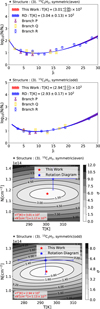 |
Fig. 7 Same as Figs. 3 and 4 but for 13C2H2 (Isotopolog “3”). For more details, we refer to the main text. |
3.3.2 12C/13C column density ratios
This section presents a comparison of 12C/13C ratios derived using the traditional RD method and the χ2 fitting method, highlighting the advantages of the latter. The 12C/13C ratios were calculated using the formula
 (13)
(13)
where N(Ortho - C2H2) and N (Para - C2H2) represent the column densities of the ortho and para states of symmetric acetylene, and N (13 CCH2) is the column density of the 13C isotopolog. This formula accounts for molecular symmetry and statistical weights, ensuring consistency and accuracy in the isotopic ratio determination.
Table 7 presents a detailed comparison of the 12C/13C isotopic ratios derived for the blue and red clumps in the Orion IRc2 using two different methods: the traditional RD method and the χ2 fitting method introduced in this study. The table also includes the absolute differences and percentage differences between the results of the two methods, highlighting the systematic biases inherent in the RD approach and the improvements achieved with the χ2 method.
For the blue clump, the χ2 method yields a 12 C/13 C ratio of  , which is approximately 12.1% lower than the RD-derived value of 21.3 ± 2.2. This difference reflects the systematic overestimation of the RD method due to its reliance on linear extrapolation and the separate fitting of temperature (T) and column density (N). Additionally, the χ2 method reduces the uncertainty of the isotopic ratio by nearly 30%, demonstrating its superior precision and reliability.
For the red clump, a hybrid approach, χ2 (12C) + RD (13C), was employed. In this approach, the χ2 method was used to determine the 12C column density, while the RD method was applied to the 13C isotopolog due to the limited number of observational data points. This combination yields a 12C/13C ratio of  which is 23.9% lower than the RD-derived value of 19.8 ± 3.4. While the χ2 method improves the overall accuracy for 12C, the use of the RD method for 13C contributes to slightly larger uncertainties compared to the blue clump.
The differences in the derived ratios are significant and underscore the importance of adopting the χ2 fitting method, which minimizes biases by simultaneously fitting T and N, incorporating statistical weights, and accounting for degeneracy factors. This method ensures more robust and accurate determination of isotopic ratios, particularly for datasets with adequate observational coverage.
Despite the limitations for the red clump, the results for both clumps confirm the systematic overestimation of 12C/13C ratios by the RD method, which could impact astrophysical interpretations of isotopic fractionation processes. The hybrid χ2 (12C) + RD (13 C) approach provides a practical solution when data for 13C is sparse, but its limitations highlight the need for more extensive observational data to fully leverage the advantages of the χ2 method.
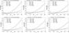 |
Fig. 8 Predicted log10(Nl/gl) values for various isotopologs of acetylene, calculated as a function of the lower rotational quantum number, Jl at four temperatures, T = 100 (solid), 300 (dashed), 500 (dotted), and 1000 (dot-dashed lines) K. The left column corresponds to 13C2H2 (Isotopolog “3”), with separate plots for even (top) and odd (bottom) rotational states. The middle column shows results for D12C13 CH (Isotopolog “4”) and D13C12CH (Isotopolog “5”), both of which are asymmetric molecules. The right column corresponds to C2D2 (Isotopolog “6”), with separate plots for even (top) and odd (bottom) rotational states. The curves are based on partition functions and energy spectra derived from quantum chemical calculations. Even states start at Jl = 0, while odd states start at Jl = 1, reflecting the symmetry properties of the isotopologs. These plots illustrate the expected population distributions across a range of temperatures, providing insights into the ro-vibrational characteristics of these acetylene isotopologs. |
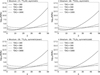 |
Fig. 9 Same as Fig. 8 but for the remaining isotopologs of acetylene. The top row shows results for asymmetric molecules: 13C2HD (Isotopolog “7”) on the left and 13CCD2 (Isotopolog “8”) on the right. The bottom row corresponds to symmetric molecules 13C2D2 (Isotopolog “9”), with even states on the left and odd states on the right. |
4 Conclusions
In this study, we have conducted a comprehensive theoretical investigation of the infrared spectra of acetylene and its isotopologs, focusing on the effects of isotopic substitution involving 13C and deuterium (D). Through extensive quantum chemical calculations using methods such as Hartree-Fock (HF), Density Functional Theory (DFT), and Møller-Plesset perturbation theory (MP2), we determined rotational constants and centrifugal distortion constants (D̃J) for molecules lacking observational data. This rigorous approach allowed us to systematically account for all possible isotopologs of acetylene, including combinations of 13C and D substitution. While 13C substitution induces subtle vibrational shifts on the order of a few inverse centimeters, detectable only with high-precision instruments such as SOFIA, D substitution causes significant vibrational shifts of tens of inverse centimeters due to its larger impact on the reduced mass. These differences in sensitivity and detectability underscore the importance of accurate rotational and vibrational constants in studying isotopic effects across a range of astrophysical conditions (for more details on quantum chemical computations, see Appendices B and C).
Comparisons with observational data from instruments such as SOFIA validated our computational approaches. The integration of the HITRAN database and the application of Doppler and LSR adjustments ensured the accuracy of our theoretical models. These comparisons highlighted the value of isotopolog-specific spectra in deciphering the molecular composition of astrophysical environments such as the Orion Nebula, as well as their critical role in tracing stellar nucleosynthesis and the chemical evolution of galaxies.
A significant contribution of this study lies in the application of the χ2 fitting method, which effectively addresses the limitations of the traditional RD approach. By simultaneously fitting temperature (T) and column density (N) while incorporating statistical weights, transition strengths, and degeneracy factors, the χ2 method minimizes systematic biases and improves the reliability of derived parameters. For the blue clump, the χ2 method achieved higher precision, reducing uncertainties in T and N for both even and odd rotational states of C2H2, while providing results consistent with or slightly adjusted from the RD method. Similarly, for 13CCH2, the χ2 method yielded column densities that aligned closely with the RD results, while significantly reducing the associated uncertainties. In the red clump, the χ2 method improved precision for C2H2, showing higher temperatures and slightly lower column densities compared to the RD method, accompanied by smaller error margins. However, for 13CCH2, the limited number of observational data points led to increased uncertainties in the χ2 method’s results, despite the central values being consistent with the RD method. This highlights a key limitation of the χ2 approach when applied to datasets with very few observations, as the increased number of fitting parameters exacerbates the impact of limited data on the robustness of the fit. Overall, these findings demonstrate the robustness and precision of the χ2 method for deriving physical parameters from molecular spectra, particularly for well-sampled datasets, while emphasizing the need for sufficient observational data to fully exploit its advantages in future studies.
Through the χ2 method, we identified systematic overestimations of 12C/13C ratios by the RD method: approximately 12.1% for the blue clump and 23.9% for the red clump. For the blue clump, the χ2 method yielded a ratio of  compared to 21.3 ± 2.2 from the RD method, with uncertainties reduced by nearly 30%. This improvement demonstrates the robustness of the χ2 method in mitigating biases and enhancing precision. For the red clump, the χ2 method estimated a ratio of
  , significantly lower than the RD-derived value of 19.8 ± 3.4. However, the uncertainty for 13CCH2 was notably larger due to the limited observational data, as explained earlier. To address this, a hybrid approach combining χ2 fitting for C2H2 and the RD method for 13 CCH2 was employed, ensuring reliable results while acknowledging the limitations of the χ2 method in sparse datasets.
In addition to demonstrating the accuracy of the χ2 fitting method, this study introduces a Python package designed to automate the spectral analysis process. The package integrates quantum chemical calculations and robust fitting techniques, enabling precise analyses of acetylene isotopologs. It supports both RD and χ2 fitting methods, providing direct comparisons and facilitating validation of results. Freely available on GitHub, the package includes precomputed rotational constants, partition functions (TIPS), and vibrational-rotational spectra for a wide range of isotopologs, addressing gaps in existing databases such as HITRAN. For details on the package’s implementation and usage, including applications to new observational data, refer to Appendix G.
In summary, this study highlights the significant advantages of the χ2 fitting method for analyzing complex molecular spectra. By reducing uncertainties and mitigating systematic biases, the method provides a robust and reliable framework for deriving isotopic ratios and molecular abundances, offering critical insights into the physical conditions of astrophysical environments. The observed systematic overestimations in isotopic ratios by the RD method underscore the need to revisit earlier studies to ensure accurate interpretations of stellar nucleosynthesis and galactic chemical evolution. Looking forward, extending the χ2 methodology to other isotopologs and molecular systems will enable more comprehensive explorations of interstellar chemistry and the mechanisms driving galactic evolution. This study not only advances our understanding of isotopic fractionation but also establishes a foundation for future high-precision spectroscopic analyses, reinforcing the importance of adopting modern data-driven approaches in astrophysical research.
Comparison of estimated temperature (T) and column density (N) values for blue and red clump species using two methods: the traditional RD method and the χ2 fitting method.
Comparison of 12C/13C isotopic ratios derived using the traditional RD method and the χ2 fitting method for the blue and red clumps in the Orion IRc2.
Data availability
The Python package TOPSEGI, developed for this study, is publicly available on GitHub at https://github.com/BrownNo28/ISM. In addition, Tables F.2–F.8 are available at the CDS via https://cdsarc.cds.unistra.fr/viz-bin/cat/J/A+A/700/A238
Acknowledgements
This work was supported by the National Research Foundation of Korea (NRF) grant funded by the Korea government (RS-2021-NR060129, RS-2022-NR070836), and we would like to express our sincere gratitude to Dr. Naseem Rangwala and Dr. Sarah Nickerson for their invaluable advice on the analysis methods for acetylene observation data. Their insights and suggestions have greatly contributed to the development and completion of this work.
Appendix A Local standard of rest and telluric corrections for infrared spectral data
To accurately interpret high-resolution infrared data, such as those obtained from SOFIA (Rangwala et al. 2018), corrections considering both the Doppler effect and LSR velocities are essential. The LSR is a coordinate system defined based on the average motion of stars near the Sun. The International Astronomical Union (IAU) defines the LSR, based on the B1900 equinox, at right ascension (α= 18 h 00 m), declination (δ= +30°) with a velocity of 20 km∕s. However, modern research uses the J2000 standard, requiring a transformation from B1900 coordinates to J2000 for analysis.
To perform LSR corrections, the Julian Date (JD) at the time of observation and the target’s RA and DEC are required to calculate the line-of-sight velocity difference between the geocentric frame and the LSR frame. This involves calculating the velocity difference between the LSR and the heliocentric (Suncentered) frame based on the defined LSR standard, adding the velocity difference between the geocentric frame and the heliocentric frame at the observation time, and combining these two differences to determine the final line-of-sight velocity between the geocentric and LSR frames.
For the observational data of the Orion IRc2 used in Fig. 2, the observation duration was relatively short at approximately 28 minutes, allowing the velocity variations over the observation period to be neglected. The Doppler effect due to the LSR was calculated to be approximately 7.29 km/s for the observational data, and Fig. 2 presents the results calculated based on the start time of the observation.
Such LSR corrections accurately account for the Doppler effects present in the observational data, providing the essential precision required for molecular spectrum analysis.
In both Rangwala et al. (2018) and Nickerson et al. (2023), the ATRAN atmospheric transmission model (Lord 1992) was used for this purpose. ATRAN has been commonly adopted for telluric correction in SOFIA/EXES observations, but it lacks recent molecular line updates and does not incorporate modern atmospheric datasets. Although we did not perform telluric correction ourselves in this study, we acknowledge these limitations, and we note that more sophisticated tools are now available. For example, the Planetary Spectrum Generator (PSG) (Villanueva et al. 2022) uses the latest HITRAN (Gordon et al. 2022) and ExoMol (Tennyson et al. 2024) databases and calculates telluric transmittances using the MERRA-2 (Gelaro et al. 2017) database, the latest atmospheric reanalysis of the modern satellite era produced by NASA. A model such as PSG, by incorporating updated molecular and atmospheric data, suggests a pathway toward more accurate telluric correction than that achievable with ATRAN.
This enables the precise determination of the observed molecular spectral line positions and facilitates the quantitative derivation of physical parameters.
Appendix B Quantum chemical calculation methods
In this study, quantum chemical calculations were performed using Gaussian16 (Foresman et al. 1996) with various computational methods to ensure the accuracy and reliability of the results. Specifically, the Hartree–Fock (HF) (Helgaker et al. 2013) method was employed for its simplicity and computational speed, providing a foundational understanding of the electronic structure. Density Functional Theory (DFT) with the B3LYP (Becke 1988; Lee et al. 1988) and PBE0 (Perdew et al. 1996) functionals was chosen for its balance between accuracy and computational efficiency, offering improved treatment of electron correlation effects compared to HF. Additionally, the second-order Møller–Plesset perturbation theory (MP2) (Møller & Plesset 1934) method was utilized to achieve higher precision in accounting for electron correlation.
Geometric optimizations were carried out using the 6-31+G* basis set, which includes polarization and diffuse functions to accurately describe molecular geometries and electronic distributions. This basis set was selected for its ability to capture the subtle effects of isotopic substitution on molecular properties.
Vibrational frequency calculations were performed for acetylene and its isotopologs, including isotopically substituted species. To evaluate the impact of isotopic substitutions, specific atoms were systematically replaced (e.g., hydrogen with deuterium or carbon-12 with carbon-13), followed by reoptimization of molecular geometries and recalculation of vibrational spectra. The changes in reduced mass due to isotopic substitution were explicitly considered to analyze their influence on vibrational frequencies.
Among the tested methods, B3LYP showed the best agreement with experimental data for most vibrational and rotational parameters, making it the primary method employed in this study. Other methods, such as HF, PBE0, and MP2, exhibited lower consistency with experimental results and were therefore not selected for further analysis.
Appendix C IR spectra and rotational constants of acetylene isotopes
We present the vibrational frequencies (ν1 ~ ν5) and the rotational constants (B̃) for acetylene (12C2H2) and its isotopologs (13C- and deuterium-substituted variants), calculated using HF, B3LYP, PBE0, and MP2 methods. Table C.1 summarizes these results, with infrared-active modes in black and inactive modes in gray. Substituted 13C or D atoms are marked with red circles to facilitate isotopolog identification. This dataset is essential for modeling isotopologs, including those not yet observed, and understanding their roles in astrophysical environments.
A frequency scaling factor (FSF) of 1.000000 was used initially for uniform comparison. For isotopologs with experimental data, the FSF was iteratively adjusted to improve agreement with observations, as detailed in sect. 3.2.1.
These parameters support the calculation of TIPS, which are critical for determining molecular column densities and isotopic ratios. Rotational constants (B̃) were validated against experimental data, demonstrating high accuracy for symmetric and asymmetric isotopologs. The results have been incorporated into the Python package developed for this study, enabling automated spectral modeling and high-resolution analyses.
Infrared vibrational frequencies (ν1, ν2, ν3, ν4, ν5) and rotational constants (B̃) for acetylene isotopologs (12C2H2, 13C-substituted, and deuterium-substituted variants) calculated using various quantum chemical methods: Hartree–Fock (HF), B3LYP, PBE0, and MP2.
Appendix D TIPS for acetylene isotopologs
Figure D.1 illustrates the temperature dependence of the TIP (Qtot) for all isotopologs of acetylene over the range of 0–1000 K. Each curve represents the partition sum calculated for each isotopolog, illustrating how isotopic substitution in both hydrogen and carbon atoms influences the partition function as temperature increases.
The plot highlights that the effect of isotopic substitution becomes more pronounced with rising temperature, as the altered mass impacts vibrational energy levels, leading to differences in the partition sum. For example, isotopologs with heavier isotopes exhibit smaller gaps between vibrational energy levels, reflected in a differing partition function.
This comparison emphasizes the role of isotopic substitution in modifying the thermodynamic properties of acetylene, providing insight into how isotopic variations affect molecular stability and energy distributions at elevated temperatures.
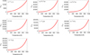 |
Fig. D.1 Temperature dependence of total internal partition sums (qtot) for various isotopologs of acetylene, displayed over a range from 0 to 1000 K. The isotopologs include 13C2H2, D12C13CH, D13C12CH, C2D2, 13C2HD, 13CCD2, and 13C2D2. Each curve represents the calculated partition sum for one isotopolog, highlighting the effect of isotopic substitution on the partition function as temperature increases. The plot emphasizes how isotopic differences in hydrogen and carbon atoms impact the thermodynamic properties of acetylene across the specified temperature range. |
Appendix E Comparison with experimental ν5 band centers and rotational constants for minor isotopologs
Table E.1 summarizes the comparison between calculated and experimentally determined ν5 band centers and rotational constants B̃ for the isotopologs not included in the HITRAN database (IDs 3–9). The calculated values were obtained from quantum chemical computations using the B3LYP method, with vibrational frequencies scaled by empirically optimized FSFs. Experimental ν5 values were extracted from high-resolution spectroscopic studies, as indicated in the rightmost column, while B̃ values for all isotopologs were consistently taken from Tamassia et al. (2016).
The relative errors, defined as (TOPSEGI - Experiment) × 100/Experiment, are found to be remarkably low–typically within 0.5% for both ν5 and B̃. This high level of agreement quantitatively confirms the accuracy of our vibrational and rotational parameter estimates, thereby supporting the reliability of the extrapolated line lists used for isotopologs lacking complete spectroscopic databases.
For ID 7 (13C2HD), the ν5 band center was not directly reported, but was instead reconstructed as the vibrational energy difference ∆G0 = G0(0,0, I, ±1) - G0(0,0,0,0) using fitted spectroscopic constants. Here, G0(v4,l4, v5,l5) denotes the vibrational term value with vi and li representing the vibrational normal modes quantum numbers and vibrational angular momentum quantum numbers of the degenerate bending modes ν4 and ν5, respectively. The convention (v4,14,v5,15) is adopted throughout, consistent with standard spectroscopic practice.
Comparison of calculated and experimental ν5 band centers and rotational constants B̃ for isotopolog IDs 3–9.
Appendix F Line list
A spectroscopic line list is a catalog of transitions that includes transition frequencies (or wavenumbers) and line strengths (or Einstein A coefficients). It also provides the lower state energy and the total state degeneracy, which are required to simulate absorption or emission spectra at various temperatures (Yurchenko & Tennyson 2014). To construct the spectroscopic line list, the line intensity was computed using the following expression (Villanueva et al. 2022):
![Mathematical equation: S(T_0) = \frac{C_{iso}}{8 \pi c} \frac{A}{\tilde{\nu}_0^2} \frac{g_u}{Q(T_0)} exp \left( -\frac{hcE_l}{kT_0} \right) \left[ 1-exp \left( -\frac{hc\tilde{\nu}_0}{kT_0} \right) \right].](/articles/aa/full_html/2025/08/aa54316-25/aa54316-25-eq43.png) (F.1)
(F.1)
In this expression, S is the line intensity at T0 = 296 K, in units of cm/molecule, Ciso is the isotopic abundance fraction, A is the Einstein coefficient in s−1, ν0 is the line center wavenumber in cm−1, gu is the upper state statistical weight, Q(T0) is the partition function at T0 = 296 K, and El is the lower state energy in cm−1. The Einstein coefficient was calculated from the vibrational transition dipole moment using the following expression (Giesen et al. 2020; Mandin et al. 2000; Lyulin & Campargue 2017):
 (F.2)
(F.2)
Here, µv is the vibrational transition dipole moment in Debye, F(Jl)(P/Q/R) is the Herman-Wallis factor, whose effective parameters are empirically deduced by expanding |μv|2 to account for the rotational dependence, and HLP/Q/R are the Hönl-London factors corresponding to the P, Q, and R branches. However, the Herman–Wallis factor was applied only to 12C2H2, for which the factor has been confirmed in the literature (Mandin et al. 2000), and was not considered for the other acetylene isotopologs. The line center wavenumber was then obtained from the energy difference between upper and lower levels:
 (F.3)
(F.3)
![Mathematical equation: E_l = \tilde{B} J_l (J_l + 1) - \tilde{D} \left[J_l (J_l + 1)\right]^2.](/articles/aa/full_html/2025/08/aa54316-25/aa54316-25-eq46.png) (F.4)
(F.4)
![Mathematical equation: E_u = \tilde{B}' J_u (J_u + 1) - \tilde{D}' \left[J_u (J_u + 1)\right]^2.](/articles/aa/full_html/2025/08/aa54316-25/aa54316-25-eq47.png) (F.5)
(F.5)
In these expressions, the ν5 frequency obtained from the B3LYP calculation was rescaled using the FSF value. The constants B̃′, and D̃, are the rotational and centrifugal distortion constants for the upper level. The values of B̃′, and D̃, were adjusted to best fit the observed ν5 band spectra in HITRAN for C2H2, 13CCH2, and C2HD, through fitting procedures applied to the P, Q, and R branches. The values of B′, for other isotopologs were estimated by multiplying the B3LYP calculated B̃ values with the B̃′/B̃ ratios derived from isotopolog IDs 0, I, and 2. The applied B′/B̃ values were grouped according to structural similarity with isotopolog IDs 0, 1, and 2, corresponding to groups (3, 6, 9), (8), and (4, 5, 7), respectively. Assuming LTE, the calculated line intensities were normalized to the total intensity using the following relation:
![Mathematical equation: \frac{S(T_0)}{\sum S(T_0)} \!=\!\! \frac{ g_i \tilde{\nu}_0 HL_{(P/Q/R)} F(J_{l})_{(P/Q/R)} exp \left( -\frac{hcE_l}{kT_0} \right) \left[ 1-exp \left( -\frac{hc\tilde{\nu}_0}{kT_0} \right) \right] } { \sum g_i \tilde{\nu}_0 HL_{(P/Q/R)} F(J_{l})_{(P/Q/R)} exp \left( -\frac{hcE_l}{kT_0} \right) \left[ 1-exp \left( -\frac{hc\tilde{\nu}_0}{kT_0} \right) \right] } .](/articles/aa/full_html/2025/08/aa54316-25/aa54316-25-eq48.png) (F.6)
(F.6)
The line intensities in the line list were obtained by multiplying the normalized intensity (Eq. (F.6)) by the corresponding  values listed in Table F.1. For isotopolog IDs 0-2, both Ciso and
  were taken from the HITRAN database, and Fig F.1–F.3 illustrate a comparison between the line intensities provided by HITRAN and those calculated in TOPSEGI (this work). The relative error, calculated as (STOPSEGI - SHITRAN) × 100/Shitran, reaches up to 40% in the range of Jl ≤ 50, but remains within 2% in the observational range (Jl ≤ 24).
These results suggest that the line intensities calculated in TOPSEGI (this work) appear reliable within the observational regime. For isotopolog IDs 3-9,  values were derived from B3LYP calculations, and Ciso was set to 1. The S values calculated from these were provided as line lists in Tables F.2–F.8, which are available only in electronic form via the CDS (see Sect. Data availability).
Estimated constants for line intensity calculation.
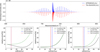 |
Fig. F.1 Comparison of line intensities in the ν5 band of C2H2 between HITRAN data (blue) and the present calculations using TOPSEGI (red). The top panel shows the full simulated band profile in terms of line intensity versus wavenumber, illustrating overall agreement in line positions and relative strengths. The bottom three panels display the relative intensity errors as a function of rotational quantum number Jl in the P, Q, and R branches, respectively. The deviation increases toward high-Jl lines, but this is consistent with limitations in the HITRAN reference intensities and the harmonic dipole approximation used in the present model. Here, the vertical lines identify the highest-Jl observed, with corresponding deviations reaching up to approximately 2%. |
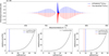 |
Fig. F.2 Same as Fig. F.1 but for 13CCH2. The vertical lines identify the highest-Jl observed, with corresponding deviations reaching up to approximately 0.3%, while the relative intensity errors reach up to approximately 36% across all branches. |
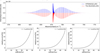 |
Fig. F.3 Same as Fig. F.1 but for C2HD. Observational data for C2HD were not used in this study, and the relative intensity errors reach up to approximately 30% across all branches. |
Appendix G Python package: TOPSEGI
TOPSEGI is a Python-based package developed to calculate the temperature and column density of molecules and molecular isotopologs constituting the atmospheres of planets, satellites, comets, and carbon stars, as well as ISM regions such as Orion IRc2.
The ISM refers to all types of gas, dust, and other components present between stars, primarily composed of interstellar dust and gas.
To represent ISM such as Orion IRc2, which is one of the key focuses of our research, we named the package TOPSEGI, a term from a central Korean dialect meaning “dust” or “tiny particles.”
While the current version supports only acetylene and its isotopologs, future updates will include the analysis of other molecules commonly found in space, such as HCN and 60C.
The package integrates advanced quantum chemical calculations with robust spectral fitting techniques, offering a userfriendly framework for determining temperature (T) and column density (N) directly from observational data. It is designed to streamline the analysis process and enhance precision, particularly for isotopologs in environments with sufficiently high isotopic ratios, such as carbon-rich stars.
The package includes precomputed theoretical data for 10 isotopologs of acetylene, covering partition functions (TIPS), rotational constants, vibrational-rotational energy levels (El)3, degeneracy factors (gl), and transition branches(see Table G.1).
TIPS are provided for a temperature range of 1–1000 K at 1 K intervals, with values available through linear interpolation within this range. Additionally, for the P, Q, and R branches, Jl are provided for values ranging from 0 to 50. In the absence of observational data, the package provides N/Nl values as a function of temperature based on theoretical data. When observational data are available, as shown in Fig. G.1, the package utilizes a Quadtree algorithm to efficiently determine T∗ and N∗ values, ensuring accurate and reliable results.
This tool supports both the traditional RD method and the χ2 fitting method introduced in this study. It allows users to perform both analyses automatically and directly compare the results, highlighting the improvements achieved with the χ2 method in terms of precision and bias reduction. Furthermore, the package enables users to assess systematic biases in isotopic ratio derivations when using different methodologies, offering valuable insights into the reliability of observational results.
The package also addresses a critical gap in current spectral databases, such as HITRAN, by providing accurate theoretical data for isotopologs not included in these resources. This capability extends the applicability of the package to future observations of diverse isotopologs, enabling rapid and reliable modeling of isotopic effects. Additionally, the precomputed theoretical data included in the package ensures consistency in analyses and eliminates the need for users to perform their own quantum chemical calculations, saving time and computational resources.
This package represents an important step forward in the study of interstellar chemistry and isotopic fractionation. By enabling the seamless application of the χ2 method to new datasets, it equips researchers with a powerful tool to analyze molecular spectra and explore the dynamic processes shaping astrophysical environments. Future updates to the package aim to include additional isotopologs and molecules, extending its usability to a broader range of applications in astrophysics and molecular spectroscopy.
Input data format required for the Python package.
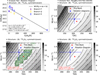 |
Fig. G.1 TOPSEGI processing steps using pseudo data of 13C2D2 with even parity. Top-left: RD constructed from observed values (Table G.1). Top-right: approximate minimum χ2 identified in T–N parameter space. Bottom-left and bottom-right: parameter space refined using quadtree approach, with best-fit values T* and N* determined. |
References
- Amyay, B., Fayt, A., & Herman, M. 2011, J. Chem. Phys., 135, 234305 [Google Scholar]
- Becke, A. D. 1988, PhRvA, 38, 3098 [Google Scholar]
- Bézard, B., Vinatier, S., Greathouse, T., et al. 2022, in European Planetary Science Congress, EPSC2022-363 [Google Scholar]
- Brooke, T., Tokunaga, A., Weaver, H., et al. 1996, Natur, 383, 606 [Google Scholar]
- Bézard, B., Romani, P. N., Conrath, B. J., & Maguire, W. C. 1991, JGRA, 96, 18961 [Google Scholar]
- Canè, E., Cazzoli, G., Di Lonardo, G., et al. 2002, JMoSp, 216, 447 [Google Scholar]
- Chubb, K. L. 2018, PhD thesis, UCL (University College London) [Google Scholar]
- Chubb, K. L., Joseph, M., Franklin, J., et al. 2018, JQSRT, 204, 42 [Google Scholar]
- Chubb, K. L., Tennyson, J., & Yurchenko, S. N. 2020, MNRAS, 493, 1531 [NASA ADS] [CrossRef] [Google Scholar]
- de Graauw, T., Feuchtgruber, H., Bezard, B., et al. 1997, A&A, 321, L13 [NASA ADS] [Google Scholar]
- El Idrissi, M. I., Liévin, J., Campargue, A., & Herman, M. 1999, J. Chem. Phys., 110, 2074 [Google Scholar]
- Encrenaz, T., Feuchtgruber, H., Atreya, S. K., et al. 1998, A&A, 333, L43 [NASA ADS] [Google Scholar]
- Esposti, C. D., Dore, L., Fusina, L., & Tamassia, F. 2013, MolPh, 111, 896 [Google Scholar]
- Fayt, A., Robert, S., Di Lonardo, G., et al. 2007, J. Chem. Phys., 126, 114303 [Google Scholar]
- Fernique, P., Allen, M. G., Boch, T., et al. 2015, A&A, 578, A114 [NASA ADS] [CrossRef] [EDP Sciences] [Google Scholar]
- Fischer, J., Gamache, R., Goldman, A., Rothman, L., & Perrin, A. 2003, JQSRT, 82, 401 [Google Scholar]
- Fonfría, J. P., Cernicharo, J., Richter, M. J., & Lacy, J. H. 2008, ApJ, 673, 445 [CrossRef] [Google Scholar]
- Foresman, J., Frisch, A., & Gaussian, I. 1996, Exploring Chemistry with Electronic Structure Methods (Gaussian, Incorporated) [Google Scholar]
- Fusina, L., Canè, E., Tamassia, F., Baldan, A., & Di Lonardo, G. 2011, JMoSp, 268, 226 [Google Scholar]
- Fusina, L., Canè, E., Tamassia, F., Villa, M., & Di Lonardo, G. 2014, MolPh, 112, 1123 [Google Scholar]
- Gamache, R. R., Hawkins, R. L., & Rothman, L. S. 1990, JMoSp, 142, 205 [Google Scholar]
- Gamache, R. R., Vispoel, B., Rey, M., et al. 2021, JQSRT, 271, 107713 [NASA ADS] [CrossRef] [Google Scholar]
- Gelaro, R., McCarty, W., Suárez, M. J., et al. 2017, JCli, 30, 5419 [Google Scholar]
- Giesen, T. F., Mookerjea, B., Fuchs, G. W., et al. 2020, A&A, 633, A120 [NASA ADS] [CrossRef] [EDP Sciences] [Google Scholar]
- Goldsmith, P. F., & Langer, W. D. 1999, ApJ, 517, 209 [Google Scholar]
- Gordon, I., Rothman, L., Hargreaves, R., et al. 2022, JQSRT, 277, 107949 [CrossRef] [Google Scholar]
- Helgaker, T., Jorgensen, P., & Olsen, J. 2013, Molecular Electronic-Structure Theory (Wiley) [Google Scholar]
- Herman, M. 2007, MolPh, 105, 2217 [Google Scholar]
- Herman, M., & Lievin, J. 1982, JChEd, 59, 17 [Google Scholar]
- Herman, M., Campargue, A., El Idrissi, M. I., & Vander Auwera, J. 2003, JPCRD, 32, 921 [Google Scholar]
- Herman, M., Depiesse, C., Di Lonardo, G., et al. 2004, JMoSp, 228, 499 [Google Scholar]
- Huet, T., Herman, M., & Johns, J. W. 1991, J. Chem. Phys., 94, 3407 [Google Scholar]
- Jacob, A. M., Menten, K. M., Wiesemeyer, H., et al. 2020, A&A, 640, A125 [EDP Sciences] [Google Scholar]
- Jacquemart, D., Mandin, J.-Y., Dana, V., et al. 2003, JQSRT, 82, 363 [Google Scholar]
- Karakas, A. I. 2010, MNRAS, 403, 1413 [NASA ADS] [CrossRef] [Google Scholar]
- Lambert, D. L., Gustafsson, B., Eriksson, K., & Hinkle, K. H. 1986, ApJS, 62, 373 [Google Scholar]
- Laraia, A. L., Gamache, R. R., Lamouroux, J., Gordon, I. E., & Rothman, L. S. 2011, Icar, 215, 391 [Google Scholar]
- Lee, C., Yang, W., & Parr, R. G. 1988, PhRvB, 37, 785 [Google Scholar]
- Lord, S. D. 1992, A New Software Tool for Computing Earth’s Atmospheric Transmission of Near-and Far-infrared Radiation, 103957 (Ames Research Center) [Google Scholar]
- Lyulin, O., & Campargue, A. 2017, JQSRT, 203, 461 [Google Scholar]
- Mandin, J.-Y., Dana, V., & Claveau, C. 2000, JQSRT, 67, 429 [Google Scholar]
- McCarthy, M. C., Gottlieb, C. A., & Cernicharo, J. 2019, JMoSp, 356, 7 [Google Scholar]
- McQuarrie, D. 2008, Quantum Chemistry, G – Reference, Information and Interdisciplinary Subjects Series (University Science Books) [Google Scholar]
- Møller, C., & Plesset, M. S. 1934, PhRv, 46, 618 [Google Scholar]
- Nickerson, S., Rangwala, N., Colgan, S. W. J., et al. 2023, ApJ, 945, 26 [NASA ADS] [CrossRef] [Google Scholar]
- Nixon, C., Achterberg, R., Conrath, B., et al. 2007, Icar, 188, 47 [Google Scholar]
- O’Dell, C. R. 2001, ARA&A, 39, 99 [Google Scholar]
- Pagel, B. E. J. 2009, Nucleosynthesis and Chemical Evolution of Galaxies (Cambridge University Press) [Google Scholar]
- Pentsak, E. O., Murga, M. S., & Ananikov, V. P. 2024, ESC, 8, 798 [Google Scholar]
- Perdew, J. P., Burke, K., & Ernzerhof, M. 1996, PhRvL, 77, 3865 [Google Scholar]
- Predoi-Cross, A., Herman, M., Fusina, L., & Di Lonardo, G. 2012, MolPh, 110, 2621 [Google Scholar]
- Protasevich, A. E., & Nikitin, A. V. 2025, JQSRT, 333, 109337 [Google Scholar]
- Rangwala, N., Colgan, S.W. J., Gal, R. L., et al. 2018, ApJ, 856, 9 [NASA ADS] [CrossRef] [Google Scholar]
- Stahler, S., & Palla, F. 2008, The Formation of Stars (Wiley) [Google Scholar]
- Tamassia, F., Cané, E., Fusina, L., & Di Lonardo, G. 2016, PCCP, 18, 1937 [Google Scholar]
- Tennyson, J., Yurchenko, S. N., Al-Refaie, A. F., et al. 2016, JMoSp, 327, 73 [Google Scholar]
- Tennyson, J., Yurchenko, S. N., Zhang, J., et al. 2024, JQSRT, 326, 109083 [Google Scholar]
- Villanueva, G. L., Liuzzi, G., Faggi, S., et al. 2022, Fundamentals of the Planetary Spectrum Generator (NASA Goddard Space Flight Center) [Google Scholar]
- Wlodarczak, G., Demaison, J., Burie, J., & Lasne, M. C. 1989, MolPh, 66, 669 [Google Scholar]
- Woods, P. M. 2010, Carbon isotope measurements in the Solar System [Google Scholar]
- Yurchenko, S. N., & Tennyson, J. 2014, MNRAS, 440, 1649 [Google Scholar]
Hereafter, unless otherwise specified, the element C refers exclusively to 12C. For carbon isotopes (Woods 2010), 13C is explicitly indicated whenever it is mentioned.
More precisely,  . The terms ϵtrans and ϵelec correspond to the translational and electronic energy levels, respectively. We note that the term ϵothers may represent the nuclear spin energy (levels) and/or the interactions between the first four. We here assume that the first four are independent, and the last terms are negligible. However, we note that the energy levels cannot be independent and can become coupled to each other as the energy of the molecule increases. Since
  , translational states far outnumber rotational, vibrational, and electronic states. Typically, qelec is close to unity, while qvib and qrot range from 1 to 100, and qtrans can exceed 1020.
All Tables
Comparison of normal modes and rotational constants of various isotopologs of C2H2 between this work (B3LYP) and related studies.
Rotational constants (B̃) and centrifugal distortion constants (D̃J) for acetylene (C2H2) and its isotopologs, determined using quantum chemical calculations based on the B3LYP method.
Comparison of estimated temperature (T) and column density (N) values for blue and red clump species using two methods: the traditional RD method and the χ2 fitting method.
Comparison of 12C/13C isotopic ratios derived using the traditional RD method and the χ2 fitting method for the blue and red clumps in the Orion IRc2.
Infrared vibrational frequencies (ν1, ν2, ν3, ν4, ν5) and rotational constants (B̃) for acetylene isotopologs (12C2H2, 13C-substituted, and deuterium-substituted variants) calculated using various quantum chemical methods: Hartree–Fock (HF), B3LYP, PBE0, and MP2.
Comparison of calculated and experimental ν5 band centers and rotational constants B̃ for isotopolog IDs 3–9.
All Figures
|
Fig. 1 Location of Orion IRc2 within the BN/KL region of OMC-1, marked by the black circle (Fernique et al. 2015). |
| In the text | |
|
Fig. 2 Mid-infrared spectra of IRc2 near the Orion Nebula (M42 or NGC 1976). Upper panel: SOFIA observational data (black lines). Middle panel: C2H2 absorption lines corresponding to R-branch. Lower panel: 13CCH2 absorption lines corresponding to R-branch. Vertical lines correspond to the HITRAN database (solid), the LSR corrections (dashed), and corrections for both the LSR and Doppler effects (dash-dotted). The shading around the dash-dotted lines represents the error associated with the transformation to the LSR. |
| In the text | |
|
Fig. 3 Analysis of the ν5 band of C2H2 and 13CCH2 using the RD and the χ2 fitting methods. Left panels: plot of log10 (Nl/gl) as a function of the lower rotational quantum number Jl, Right panels: contour plots from the χ2 method. In the left panels, purple triangles, yellow rectangles, and blue circles indicate observational results for the P-, Q-, and R-branches, respectively, based on the Nickerson et al. (2023) study of Orion IRc2. Each point includes 1σ error bars. The blue shaded regions represent the 1σ uncertainty range for the RD method, with the blue solid line showing the best-fit result. The red line represents results from the χ2 method, providing more precise estimates of physical parameters. The right panels display contour plots illustrating the confidence intervals for the χ2 method with two degrees of freedom, temperature (K) and column density (molecules per square centimeter). The contours depict the difference between observed and theoretical lower-state column densities (Nl), with the minimum value indicating the best-fit parameters. The red star marks the best-fit temperature and column density from the χ2 method, while blue stars with error bars denote the RD best-fit values with 1σ uncertainties. Contour levels correspond to confidence levels, and the explicit best-fit values of T and N are displayed in red in the lower-left corner. These results emphasize the improved accuracy of the χ2 fitting method (right panels) compared to the RD approach (left panels) in determining the physical properties of the blue clump component. Additionally, the X-shaped hatching in the right panels indicates regions where ∆χ2 is too large, making numerical calculations infeasible. |
| In the text | |
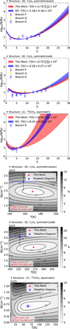 |
Fig. 4 Same as Fig. 3, but for the red clump. |
| In the text | |
|
Fig. 5 Comparison of calculated log10(Nl/gl) values for C2HD as a function of the lower rotational quantum number Jl at different temperatures (T = 100 (solid), 300 (dashed), 500 (dotted), and 1000 (dot-dashed) K). The red lines represent the values using our calculated TIP function, while the blue lines correspond to the reference results using the HITRAN TIP function. The agreement between this work and HITRAN validates the accuracy of the current method, particularly at higher temperatures, where deviations are minimal. |
| In the text | |
|
Fig. 6 Comparison of the total internal partition sums (Qtot) as a function of temperature for acetylene (C2H2), 13 CCH2, and C2HD. The solid blue line represents the results from this work, while the red dashed line shows the HITRAN values. The agreement between our calculations and HITRAN demonstrates the accuracy of our method across a wide temperature range (0–1000 K). |
| In the text | |
|
Fig. 7 Same as Figs. 3 and 4 but for 13C2H2 (Isotopolog “3”). For more details, we refer to the main text. |
| In the text | |
|
Fig. 8 Predicted log10(Nl/gl) values for various isotopologs of acetylene, calculated as a function of the lower rotational quantum number, Jl at four temperatures, T = 100 (solid), 300 (dashed), 500 (dotted), and 1000 (dot-dashed lines) K. The left column corresponds to 13C2H2 (Isotopolog “3”), with separate plots for even (top) and odd (bottom) rotational states. The middle column shows results for D12C13 CH (Isotopolog “4”) and D13C12CH (Isotopolog “5”), both of which are asymmetric molecules. The right column corresponds to C2D2 (Isotopolog “6”), with separate plots for even (top) and odd (bottom) rotational states. The curves are based on partition functions and energy spectra derived from quantum chemical calculations. Even states start at Jl = 0, while odd states start at Jl = 1, reflecting the symmetry properties of the isotopologs. These plots illustrate the expected population distributions across a range of temperatures, providing insights into the ro-vibrational characteristics of these acetylene isotopologs. |
| In the text | |
|
Fig. 9 Same as Fig. 8 but for the remaining isotopologs of acetylene. The top row shows results for asymmetric molecules: 13C2HD (Isotopolog “7”) on the left and 13CCD2 (Isotopolog “8”) on the right. The bottom row corresponds to symmetric molecules 13C2D2 (Isotopolog “9”), with even states on the left and odd states on the right. |
| In the text | |
|
Fig. D.1 Temperature dependence of total internal partition sums (qtot) for various isotopologs of acetylene, displayed over a range from 0 to 1000 K. The isotopologs include 13C2H2, D12C13CH, D13C12CH, C2D2, 13C2HD, 13CCD2, and 13C2D2. Each curve represents the calculated partition sum for one isotopolog, highlighting the effect of isotopic substitution on the partition function as temperature increases. The plot emphasizes how isotopic differences in hydrogen and carbon atoms impact the thermodynamic properties of acetylene across the specified temperature range. |
| In the text | |
|
Fig. F.1 Comparison of line intensities in the ν5 band of C2H2 between HITRAN data (blue) and the present calculations using TOPSEGI (red). The top panel shows the full simulated band profile in terms of line intensity versus wavenumber, illustrating overall agreement in line positions and relative strengths. The bottom three panels display the relative intensity errors as a function of rotational quantum number Jl in the P, Q, and R branches, respectively. The deviation increases toward high-Jl lines, but this is consistent with limitations in the HITRAN reference intensities and the harmonic dipole approximation used in the present model. Here, the vertical lines identify the highest-Jl observed, with corresponding deviations reaching up to approximately 2%. |
| In the text | |
|
Fig. F.2 Same as Fig. F.1 but for 13CCH2. The vertical lines identify the highest-Jl observed, with corresponding deviations reaching up to approximately 0.3%, while the relative intensity errors reach up to approximately 36% across all branches. |
| In the text | |
|
Fig. F.3 Same as Fig. F.1 but for C2HD. Observational data for C2HD were not used in this study, and the relative intensity errors reach up to approximately 30% across all branches. |
| In the text | |
|
Fig. G.1 TOPSEGI processing steps using pseudo data of 13C2D2 with even parity. Top-left: RD constructed from observed values (Table G.1). Top-right: approximate minimum χ2 identified in T–N parameter space. Bottom-left and bottom-right: parameter space refined using quadtree approach, with best-fit values T* and N* determined. |
| In the text | |
Current usage metrics show cumulative count of Article Views (full-text article views including HTML views, PDF and ePub downloads, according to the available data) and Abstracts Views on Vision4Press platform.
Data correspond to usage on the plateform after 2015. The current usage metrics is available 48-96 hours after online publication and is updated daily on week days.
Initial download of the metrics may take a while.