| Issue |
A&A
Volume 700, August 2025
|
|
|---|---|---|
| Article Number | A213 | |
| Number of page(s) | 14 | |
| Section | Galactic structure, stellar clusters and populations | |
| DOI | https://doi.org/10.1051/0004-6361/202554531 | |
| Published online | 19 August 2025 | |
C and N abundances in globular clusters
I. The case of 47 Tuc (NGC 104) and the effect of the first dredge-up: Implications for the isochrone fitting
1
Universidad Andres Bello, Facultad de Ciencias Exactas, Departamento de Física y Astronomía – Instituto de Astrofísica,
Autopista Concepción-Talcahuano 7100,
Talcahuano,
Chile
2
INAF-Osservatorio Astronomico di Trieste,
Via G.B. Tiepolo 11,
34143
Trieste,
Italy
3
Osservatorio Astronomico di Padova-INAF,
Vicolo dell’Osservatorio 5,
35122
Padova,
Italy
4
Departamento de Astronomía, Casilla 160-C, Universidad de Concepción,
Concepción
4030000,
Chile
5
Las Cumbres Observatory
6740 Cortona Drive, Suite 102
Goleta,
CA
93117,
USA
6
Department of Geology,
Sölvegatan 12,
Lund,
Sweden
★ Corresponding author: This email address is being protected from spambots. You need JavaScript enabled to view it.
Received:
14
March
2025
Accepted:
4
June
2025
Abstract
Context. Globular clusters exhibit star-to-star chemical variations that are traceable through both photometric and spectroscopic data. While UV photometry and light-elements such as Na and O are commonly used for this purpose, the optical V versus (V-I) color– magnitude diagram (CMD) is often assumed to be relatively unaffected by such inhomogeneities and is used to derive basic cluster parameters. On the other hand, C and N would be the best chemical tracers of these variations but are challenging to measure due to their spectral features lying in the blue/UV or IR regions.
Aims. In this study, we investigate chemical variations in the globular cluster NGC104 (47Tucanae) while aiming to trace multiple stellar populations across evolutionary phases and examining how the C/N anti-correlation evolves from the main sequence (MS) to the asymptotic giant branch (AGB). We also assess the impact of these populations on the interpretation of the V versus V-I diagram.
Methods. Using spectra spanning all evolutionary stages, we derived [C/Fe] and [N/Fe] abundances for a large stellar sample. These abundance measurements were inferred from the CN and the CH features, while atmospheric parameters are homogeneously derived from photometry. The inferred abundances allowed us to disentangle multiple populations along the CMD and refine cluster parameters.
Results. We find that MS stars are more C and N-rich than their red giant branch, horizontal branch, and AGB counterparts. The C/N anticorrelation shifts during the sub-giant branch phase, coinciding with the first dredge-up, after which C decreases by 0.15–0.20 dex, N by ∼0.1 dex, while Fe remains unchanged. Interestingly, stars with different C and N abundances occupy distinct regions of the V vs V-I diagram, a pattern not attributable to differential reddening. Proper CMD fitting requires two isochrones with differing helium content, metallicity, and possibly age.
Key words: Galaxy: abundances / globular clusters: individual: NGC 104
© The Authors 2025
 Open Access article, published by EDP Sciences, under the terms of the Creative Commons Attribution License (https://creativecommons.org/licenses/by/4.0), which permits unrestricted use, distribution, and reproduction in any medium, provided the original work is properly cited.
This article is published in open access under the Subscribe to Open model. This email address is being protected from spambots. You need JavaScript enabled to view it. to support open access publication.
1 Introduction
Galactic globular clusters (GCs) are known to host star-to-star variations of their chemical content. More specifically, Carretta et al. (2009) showed that all Galactic GCs have at least a spread (or anti-correlation) in the content of their light-elements O and Na. In some case, a Mg and Al spread is also observed (Pancino et al. 2017). The only confirmed exception is Ruprecht 106, where Villanova et al. (2013) found that stars show no variation. This spread is due to the early evolution of each cluster, formed initially by a first generation of stars that has the same chemical composition of field stars at the same metallicity. The subsequent generation of stars (Na-richer and O-poorer) is formed from gas polluted by ejecta of evolved stars of the first generation (Na-poorer and O-richer). This is the so-called multiplepopulation (MP) phenomenon. This spectroscopic evidence has been interpreted as the signature of material processed during H-burning at high temperatures by proton-capture reactions (such as the Ne–Na and Mg–Al cycles). Several polluters have been proposed: intermediate-mass asymptotic giant branch stars (D’Antona et al. 2016), fast-rotating massive stars (Decressin et al. 2007), and massive binaries (De Mink et al. 2009). An attractive alternative has been proposed by Bastian et al. (2013) that implies only a single burst of star formation. They postulate that the gas ejected from massive stars of the first (and only) generation concentrates in the center of the cluster and is acquired by low-mass stars via disk accretion while they are in the fully convective phase of the pre-main sequence. However, none of the proposed scenarios can account for all observational constrains, as explained by Renzini et al. (2015).
In addition to the abundance spread of light elements, variations in heavier elements have also been found in some massive GCs, such as ω Centauri (Villanova et al. 2014), M54 (Carretta et al. 2010), M22 (Marino et al. 2009), Terzan5 (Massari et al. 2014), and NGC 2419 (Cohen et al. 2010). However, these are generally thought to be the vestiges of more massive primitive dwarf galaxies that merged with the Galaxy.
Parallel to the spectroscopic evidence, although found much later, an unexpected multiplicity in their color-magnitude diagram (CMD) sequences was discovered (e.g., Piotto et al. 2007 for NGC2808, Milone et al. 2008 for NGC1851, and Anderson et al. 2009 for 47Tuc). Dedicated mid-/near-ultraviolet Hubble Space Telescope surveys (Piotto et al. 2015; Milone et al. 2017; Nardiello et al. 2018) ultimately proved that multiplicity in the main sequence, the sub-giant branch and the red giant branch is the general rule rather than an exception.
Based on the observation stated above, we can conclude that optical Na-O abundances and UV photometry have been the key observable to disentangle MP in GCs, at least until the advent of infrared instruments and surveys, such as the APOGEE (Majewski et al. 2017) and CAPOS (Geisler et al. 2021) surveys. These surveys allow for measurement of carbon and nitrogen abundances, for which the access in the optical is forbidden most of the times for the two reasons. In metal poor stars, such as most of the targets in GCs, carbon can be measured only from the G-band at 4300 Å. This spectral region is not included in most of the default setups that have been used to study MPs, such as the UVES-580nm or the GIRAFFE-HR11/HR13 at the FLAMES instrument of the VLT, and dedicated observations must be planned. Also, good N abundance estimations can be done only in the blue-UV region (that is, the blue CN 4125 Å or other even bluer CN bands) or in the near IR, beyond 8000 Å. The second reason is that blue and UV spectra are heavily crowded making abundance determination difficult, even with the use of spectrosynthesis and the up-to-date molecular linelists.
As the APOGEE and CAPOS surveys shown, C and N abundances are very powerful tools to study MPs since the N variation in GC stars is extreme. Most of the time this variation is larger than 1 dex, and this makes the separation of the sub-populations much easier compared to O or Na. However, the use of C and N has two limitations. The first is that it must always be coupled with a determination of the O abundances for stars colder than 4500 K where, due to the molecular equilibrium, the three atoms form CO, OH, CN, and CH molecules. This is easy in the IR, where several OH lines are present in the giant stars that are the targets of the two surveys (we must note however, that OH lines vanish rapidly when stars become hotter than 4500÷5000 K), but in the optical it requires the observation of the only O line at 6300 Å, which is very far away from the CN and CH bands. The second limitation is that surface C and N abundances are supposed to change, moving from the MS to the red-giant branch (RGB) due to the effect of the first dredge-up (Salaris et al. 2020). This effect is poorly studied, and it makes difficult to assess the original abundances of the sub-populations.
NGC 104, or 47 Tuc, is one of the most massive GCs in the Milky Way (Baumgardt & Hilker 2018), and it has been studied by several authors. The classical Carretta et al. (2009) paper found the typical Na-O anticorrelation, while Norris & Freeman (1982), using low resolution spectra of a sample of HB stars, found the presence of a C versus N anticorrelation, with C-poor stars redder on average and 0.04 fainter in their V magnitude. This result was later confirmed by Briley (1997). Finally Milone et al. (2012) showed that the cluster has a bimodal CMD where two populations can be easily be identified using UV filters. A minor third population (8% of the total) can also be seen at the level of the sub-giant branch (SGB).
In this paper, we will use blue and UV spectroscopic data to trace the C and N abundances. These data cover the full CMD, from the main sequence (MS) to the asymptotic giant branch (AGB), so we are able to trace the [C/Fe] and [N/Fe] variation in all the evolutionary phases, including the SGB, where the first dredge-up is supposed to happen. We have a collection of low, middle, and high resolution spectra and high quality V versus VI photometry that allow us to estimate homogeneous atmospheric parameters along the entire CMD. In this context, the most difficult parts to study are the MS and the turn-off (TO) because their targets are intrinsically faint but also because, for such hot stars (Teff ~ 6000 K), the CN feature at 4215 Ǻ, which can be used in the more advances phases, is no longer visible, and the UV CN band at 3870 Å must be considered. However, this band (and the carbon G-band at 4300 Å) is easily resolved in low resolution spectra, which also allows one to obtain high S/N data for such faint targets.
Our investigation also led us to a deeper understanding of the V versus V-I CMD. As mentioned earlier, UV photometry is used to separate MPs in GCs since the sub-population occupy different loci in UV CMDs. On the other hand the V versus V-I or analogous CMDs have always been used to infer the basic parameters of the clusters, such as the age, the distance, and reddening (Marino et al. 2009), since FG and SG are generally assumed to be well mixed there. The only exception we know of is Anderson et al. (2009), who found an intrinsic spread in the NGC 104 MS 3 magnitudes below the TO and a split in the SGB region. We show that, thanks to our spectroscopic data, MPs can be disentangled in all the evolutionary phases also in the V versus V-I CMD, and this has an important impact in the parameter determination of the cluster.
In Sections 2 and 3, we describe the data we used and the first spectroscopic analysis. Section 4 shows how C and N abundances can be used to disentangle MPs from the MS to the AGB and how better parameters for the cluster can be obtained. This also allowed us to obtain better atmospheric parameters for the targets, and in Section 5 we perform a second data analysis using these improved parameters. In Section 6, we discuss the results, and we give a summary in Section 7.
2 The data
The data we used in this paper were obtained from different sources. As far as photometry is concerned, we used groundbased data provided by Stetson et al. (2019)1 and HST data from the HST Large Legacy Treasury Program (Piotto et al. 2015; Nardiello et al. 2018)2. The ground-based photometry covers a radial range from ~2′ to ~25′ (see Figure 1) in the B, V and I filters, and spans from the tip of the RGB to well below the main-sequence turnoff point. HST photometry is based on data obtained using the F275W, F336W, F438W, F606W, and F814W filters in the central 4′ × 4′ region (see Figure 1) and spans from the tip of the RGB to several magnitudes below the main-sequence turnoff point. We complemented ground-based photometry with Gaia DR3 (Gaia Collaboration 2016; Gaia Collaboration 2023)3 in order to have proper motions and select member stars. A summary of the photometric data we used is reported in Table 1.
Spectroscopic data for the MS/SGB region were kindly provided by Daniel-Rolf Harbeck (priv. commun.) and are those published and described in Harbeck et al. (2003) and Briley et al. (2004), while data for the RGB/HB/AGB region were obtain by the ESO program 105.2094.001 (PI: Momany). The MS/SGB spectra (for 115 targets in total) were obtained at the ESO VLT telescope using multi-slit masks with the Focal Reducer and Low Dispersion Spectrograph 2 (FORS2)4 and cover a range from 3800 to 5500 Å with a resolution of R=815. A significant fraction of these targets were rejected for the analysis because of the too low S/N or because they turned out to be non-members, leaving us with 58 targets for which good abundances have been obtained. 97 RGB/HB/AGB targets were instead observed using the FLAMES at VLT+GIRAFFE spectrograph5 with the LR02 grism and cover a range from 3964 to 4567 Å with a resolution of R=6000. The sky was clear, and the typical seeing was 0.8 arcsec. Thirty-two 45 min spectra were obtained for each target. The data were reduced using GIRAFFE pipeline 2.16.106, which corrects spectra for bias and flat-field. Then spectra were extracted and a wavelength calibration solution is applied based on nonsimultaneous calibration lamps. After that, each spectrum was corrected for its fiber transmission coefficient, which is found from flat-field images by measuring, for each fiber, the average flux relative to a reference fiber. Using IRAF7 we applied a sky correction to each stellar spectrum by subtracting the average of the 10 sky spectra that were observed simultaneously with the stars (same FLAMES plate). Finally, all of them were normalized to the continuum, i.e., divided by a low-order polynomial that fits its continuum, and the 32 spectra for each star were combined. The resulting spectra have a dispersion of 0.2 Å per pixel and a typical S/N 300–350. Of the 97 targets, 11 were not considered for the abundance analysis because they have temperature below 4500 K, which would require an oxygen abundance estimation to have reliable C and N contents, as discussed above.
The spectroscopic dataset was complemented with high-resolution spectra of 58 targets in the SGB region from the ESO program 089.D-0579 (PI: Marino). Also in this case data were obtained using the FLAMES at VLT+GIRAFFE spectrograph, but with the HR04 grism and cover a range from 4188 to 4392 Å with a resolution of R=24 000. The sky was clear, and the typical seeing was 0.8 arcsec. Eleven 45 min spectra were obtained for each target. The data were reduced using GIRAFFE pipeline 2.16.10 applying the same procedure described before. Resulting spectra have a dispersion of 0.05 Å per pixel and a typical S/N 20–60. A summary of the spectroscopic data we used is reported in Table 2.
We used the FXCOR utility within IRAF to measure the radial velocity, adopting a synthetic spectrum as a template calculated with a temperature of 5000 K, a gravity of 3.0, and a metallicity of [Fe/H]=–0.70. All the GIRAFFE targets were selected in order to be members using Gaia database, and the membership was also confirmed by radial velocities, that all agree within a dispersion of ∼10 km/s around the mean that is –16 km/s, a value very close to that given by Harris (1996), i.e. –18 km/s. All the targets are reported in Table 3 where we give the ID, the coordinates, the V and I magnitudes, proper motions, atmospheric parameters (Teff, log(g), vt), the evolutionary phase (MS,SGB,RGB,HB,AGB), the population the target belong to (FG or SG), and the carbon and nitrogen abundances (see the following sections for the determination of the atmospheric parameter, the phase, the population and the abundances).
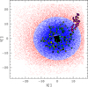 |
Fig. 1 Distribution of NGC 104 member stars in the sky. Blue and red points are stars from ground-based photometry, while black points in the center are stars from the HST Large Legacy Treasury Program. The radial cut at 15′ was used to separate the inner from the outer cluster region. Black circles with colored insets represent MS (magenta), SGB (yellow), RGB (green), HB (cyan) and AGB (black) targets (see text for more details). |
Summary of the photometric databases we used in the paper.
3 First data analysis
Our targets are plotted in Figures 1 and 2. According to their position on the CMD, we could identify 52 MS (magenta), 53 SGB (yellow), 67 RGB (green), 90 HB (cyan) and 26 AGB (black) stars. Inside each symbol of Figure 2 there is a red or blue circle which identify if the target belongs to the first or second generation respectively. This identification is discussed below, when C and N abundances are available. We anticipate that reliable C and N abundances were obtained only for those RGB/AGB targets having Teff>4500 K. This is because for lower temperatures oxygen starts to play an important role in the molecular equilibrium, and a small change of 0.1 dex in its abundance can have an impact of up to several tenths of dex in [C/Fe] or [N/Fe]. Several RGB stars were rejected but we kept an AGB star with Teff=4329 K (a temperature not far away from our limit) for completeness. In order to obtain the atmospheric parameters we decided to use the V versus V-I CMD because the V-I color depends only on temperature and not on metallicity according to Alonso et al. (1999). Then we performed an isochrone fitting using the Padova database (Bressan et al. 2012)8. We varied age and [M/H] in order to obtain the best fit of the TO and the slope of the upper RGB regions respectively, and varied the apparent distance modulus (m-M)V and the reddening E(V-I) in order to properly fit all the evolutionary phases of the CMD. The fitting was obtained by minimizing the distance between the isochrone and the photometry. For the MS and RGB phases we minimized the color difference at a given magnitude, while for the SGB, HB and AGB we minimized the magnitude difference at a given color. We also applied a visual check in order to avoid bad fitting to the data. We obtained the following preliminary parameters: (m-M)V =13.29, E(V-I)=0.03, Age=14.0 Gyrs and [M/H]=–0.60.
We notice that, while the fitting of the TO, upper MS, SGB, upper RGB, HB and AGB is quite good, the isochrone is slightly redder then the lower MS and the lower RGB. The first natural explanation would be that the isochrone has some modeling issue in those regions of the CMD but, as we show later, the correct explanation is that two isochrones with different Y and [M/H] values are required to properly fit the NGC 104 V versus V-I CMD. On the other hand, the fit we propose here is good enough for a first estimations of the parameters. According to the evolutionary phase we used two different but complementary method. Temperature for SGB and HB targets was estimated from the Teff versus V-I relation that can be obtained from the isochrone at that evolutionary phases. Gravity for HB targets was just assumed to be log(g)=2.47, since this is the value given by the isochone for unevolved HB stars, while for the SGB we used the log(g) versus V-I relation that can be obtained from the isochrone. For the MS, the RGB and the AGB instead it is possible to obtain Teff versus V and log(g) versus V relations from the isochrone that return parameters with a significantly lower internal error than the classical Teff versus V-I method, both because the V magnitude has an error  times lower than the V-I color and because such relations are intrinsically less sensitive to any internal error. As we show later, this second method return abundances that are only marginally better that the first for RGB and AGB targets, but that are significantly better for the MS, where errors on magnitudes are large for the faintness of the stars. We also show that this first guess of the parameters is affected by internal systematic errors that will be corrected using the two isochrone fitting we mentioned above. Portions of the isochrone used for the parameter determination are indicated by yellow segments in Figure 2. Having temperature and gravity for each target, microturbulence can be obtained using the relation by Mott et al. (2020). The final parameters we need for the spectral analysis is metallicity [Fe/H], for which we assumed a value of –0.70 dex (Harris 1996).
Atmospheric models were calculated using the ATLAS9 code (Kurucz 1970) assuming our initial estimations for atmospheric parameters. We then used the 2.77 version of the SPECTRUM software9 to calculate synthetic spectra. We obtained C abundance from the G band. For low resolution spectra we used the range 4280–4315 Å, while for the intermediate and high resolution spectra we used the 4300–4315 Å range. For the N abundance instead, we used the CN band at 3845–3885 Å for the low resolution spectra, while the CN band at 4214–4126 Å for the intermediate and high resolution spectra. Examples of spectrosynthesis are reported in Figure 3, while abundances are reported in Figure 4 and Table 3. For this first analysis we adopted the C and N abundances from Marino et al. (2016) as far as HR04 data are concerned. We review and refine these abundances during the second data analysis. We just notice here that Marino et al. (2016) gives no N content for a subsample of star, probably because the N feature was too weak to be measured. Since the lowest N content measured by Marino et al. (2016) is +0.2 dex, we give [N/Fe]=0.0 as upper limit to this subsample for the moment. We show in Section 5 that a reliable N content can be measure also for these targets.
A clear [N/Fe] versus [C/Fe] anticorrelation appears (see Fig. 4) with unevolved MS targets having higher C and N abundances on average if compared with their more evolved counterparts in the RGB/HB/AGB. SGB targets appear to cover both regions instead. The separation between the two groups of stars in indicated by the red line. A clear separation between first and second generation stars also appears, indicated by the black line. All stars with [N∕Fe]<0.2 dex belong to the first generation (FG), while stars with [N∕Fe]>0.2 dex belong to the second generation (SG).
At this point a possible concern is any systematic error that could affect our analysis since we used spectra with different resolutions and also different features for the nitrogen abundance determination. As far as C is concerned, we used the same feature (the G-band) although with a larger spectral interval for the low-resolution spectra of MS stars in order to have a better precision. To check a possible systematic error introduced by this choice we selected a sub-sample of 10 MS stars and determine their C content using the same narrower interval we applied to the other higher-resolutions data, i.e. 4300–4315 Å. We found that the systematic error, if present, is lower than 0.05 dex and compatible with 0. If we consider N instead, we used a completely different CN feature for low resolution MS spectra because there only the UV CN feature was measurable, while in intermediate and high resolution spectra only the CN feature at 4215 Å was visible. Unfortunately we have no stars in common between the two datasets in order to verify the present of possible systematics. However, in Fig. 4 we see that SG MS stars (the black points above the black line and on the right of the red line), whose N abundance was obtained using the UV CN feature, overlap nicely in their N content with SG SGB stars (the red points above the black line and on the right of the red line), whose N abundance was obtained using the CN feature at 4215 Å. This indicates that any systematic error, if present, is small enough not to affect our results.
Summary of the spectroscopic databases we used in the paper.
Parameters and [C/Fe] and [N/Fe] abundances for our targets.
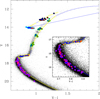 |
Fig. 2 Position on the CMD of our targets. The blue and yellow line is the best fitting isochrone we used for the parameter determination. Blue and red symbols inside each circle represent FG and SG stars respectively (see text for more details). |
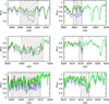 |
Fig. 3 Example of spectrosynthesis. Panels on the left show the synthesis for C while panels on the right show the synthesis for N. The upper row shows the synthesis for the MS target #1_13, the middle row shows synthesis for the HB target #RHB_I_a_40848, and the lower row shows the synthesis for the SGB target N104e_51104. The wavelength range used for the abundance determination is shown as a shaded region. Observed spectra are in green. Red spectra show the best match, while blue and black spectra represent abundance variations of ±0.5 dex for C respectively, while for N we used ±1.0 dex for low resolution spectra of MS and SGB stars (upper panel) and ±0.5 dex for intermediate and high resolution spectra of SGB, RGB, HB and AGB stars (middle and lower panel). |
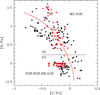 |
Fig. 4 [N/Fe] versus [C/Fe] anticorrelation as obtained from the first abundance determination run. The red line divides MS targets on the right from RGB/HB/AGB targets on the left. SGB targets are located on both sides of the red line. The black line divides FG from SG stars. Red arrows indicate stars for which Marino et al. (2016) gives no [N/Fe]. For these stars we assumed [N/Fe]=0.0 as an upper limit (see text for more details). |
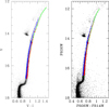 |
Fig. 5 Ground-based (left) and HST (right) CMDs of the cluster. FG generation (red) and SG (blue) star selection is indicated. The green line is the isochrone used for this selection (see text for more details). |
4 FG and SG stars in the CMD
We can now separate our targets into FG and SG stars and see where they are located on the CMD. For this purpose we indicated FG stars with red insets and SG stars with blue insets in Figure 2. We immediately observe that, as far as the RGB is concerned, FG and SG stars are clearly separated, with almost no overlap, and with SG being bluer. The color difference is on average constant and of the order of 0.03 mag. AGB and HB targets present the same behavior, but with a certain overlap. SGB targets are totally mixed while the situation for the MS is better shown in the inset plot of Figure 2. Even if FG and SG stars appear to be mixed, we can see that on average FG stars tend to follow closely the isochrone, while SG tend to be bluer, especially for V>18.4. This behavior is explained in Section 5, but we can anticipate that it is a combination of selection effects, binarity and that SG stars are 0.03–0.04 mag bluer also in MS.
We asked ourselves what is the physical cause of this bimodality in the RGB and how it can affect also the rest of the CMD. The first suspect in such cases is always differential reddening, although for this cluster this hypothesis seems to be very unlikely for two reasons. The first is the very low reddening (E(B-V)=0.03, Harris 1996) which would translate in a even lower (if not negligible) differential reddening (∆E(B-V)max=0.02, Pancino et al. 2024). The second is that, if FG and SG are intrinsically mixed in the CMD (for example in the RGB phase), it would be extremely unlikely (if not impossible) for the differential reddening to separate them in a blue RGB, composed only by SG stars, and a in red RGB, containing only FG stars. In any case we decided to dig deeper into this issue. First of all, we selected blue and red RGB stars both in the ground-based and the HST photometries (see Figure 5) and checked the spatial distribution of the two populations. In Figure 6, where we report the histogram distribution and cumulative distribution as a function of the radius of the two populations, several things can be noticed:
In the central part (within 3′) SG slightly dominated, but it appears to drop faster than FG. In any case the cumulative distributions in this regions do no differ too much.
Between 3′ and 10′ SG largely dominates.
Beyond 10′ FG starts to dominate and at 15′ almost only FG stars are present.
The cumulative distribution beyond 3′ shows that SG is more concentrated.
It is difficult to say anything about what happens at 3′ since it correspond to the transition between the two photometries, the ground-based one being largely incomplete for smaller radii.
A Kolmogorov–Smirnov test indicated that, while in the central part (within 3′) the difference between the two cumulative distributions is not significant (Dsample=0.10<Dref=0.17 at a significance level of 1%), in the outer part (beyond 3′) the FG and SG populations really have a different distribution, with the latter being more concentrated (Dsample=0.30>Dref =0.06 at a significance level of 1%).
This goes against differential reddening being the cause for the CMD dichotomy. A final check is to ask what would happen if the 0.03 V-I color separation between the two RGB is caused by differential reddening and try and correct the CMD accordingly. A ∆(V - I)=0.03 translate into a ∆(B - V)=0.025, which translates into a ∆(V)=0.07, incompatible with the SGB narrowness visible in Figure 2, that has a V spread (σ) of 0.03 magnitudes. The two values are incompatible, ruling out the possibility for differential reddening to play an important role in shaping the CMD.
Since differential reddening is not the cause of the split we see in the RGB, we have to look toward other directions. One first candidate is the abundance difference in C, N, O and He affecting the two populations. According to our first results, the FG has [C/Fe]∼–0.1 and [N/Fe]∼–0.2 while the SG has [C/Fe]∼–0.4 and [N/Fe]∼+0.6. Carretta et al. (2009) finds [O/Fe] +0.3 and +0.1 for the two populations. If we calculate a synthetic spectrum for such abundances and typical RGB parameters (Teff=5000 K, log(g)=2.50), and apply the V and I filter transmission curves given by the Asiago Database on Photometric Systems (Moro & Munari 2000)10, we obtain a color difference that is almost negligible (<<0.01 mag). We find the same result also if we apply an He variation for the second generation. In this last case we also took into account the effect of He enhancement calculating ad-hoc atmospheric models. Our simulation shows that, in order to have a color difference >0.01 mag, we have to use Y>0.40 for the second generation, a helium abundance never found in any globular cluster.
The only possibility left to explain the fact that RGB SG star are bluer is that they are intrinsically hotter. This can also be deduced from the Alonso et al. (1999) paper that, as far as the Teff versus V-I relation for giants is concerned, finds no direct relation between the color and the metallicity of a star, just between color and temperature. That means that two giants with the same temperature always have the same V-I color, even if their metallicity is different. However, the indirect cause for giant stars to be hotter is the global metal content [M/H] as can be inferred from isochrones. In fact, if we compare isochrones with different [M/H] values, the RGB part of that with the lower metallicity has higher temperatures and is bluer. For this reason the cause for SG to have a bluer RGB is that it has a lower global metallicity [M/H] or, in other words, a lower Z value. The way to prove this hypothesis is to perform a double isochrone fitting of the entire CMD. We start from the outer part where, as we have shown, we can isolate the FG. The CMD of stars having r>15′ is reported in Figure 7. As we can see, the same isochrone we used in Figure 2 is now an almost perfect fit of the data in all the evolutionary phases and all the discrepancies we mentioned in Section 3 are no longer present. We obtained the following final parameters: (m-M)V =13.24, E(V-I)=0.025, (m-M)0=13.16 (distance=4290 pc, assuming RV =3.1), Age=14.0 Gyr and [M/H]=–0.60. We also assume Y=0.0255, that gives a good fit to the lower part of the RGB, which shape is sensible to the helium content. Typical systematic uncertainties are 0.10 and 0.01 mag on the distance modulus and reddening respectively, and 0.1 dex in [M/H]. The error on age is 1 Gyr.
If we move to the central part (r<15′), FG and SG are mixed together but we can highlight the position of the SG using the Hess diagram. For this purpose we report in Figure 8 the difference of the Hess diagram of the full field photometry and the r>15′ photometry. The isochrone of Figure 2 is also reported as reference. It is clear that the SG not only has a bluer RGB, but also a bluer TO and MS. Some caution must be used with the MS, however. This is because, while the SG RGB is well detached from its FG counterpart, the SG MS is partially merged with its FG counterpart, so that the MS we see in Figure 8 is just the blue wing of the total SG MS. This fact must be taken into account for the following isochrone fitting.
In order to obtain a proper CMD fitting, we have to take also He variation into account, especially to better reproduce the lower RGB and the MS. Unfortunately this is not possible with the isochrone database we used until now, so we are forced to move to the BASTI database (Pietrinferni et al. 2021)11, which gives the possibility to use different values for Y. First of all we selected the He normal (Y=0.25) isochrone that best reproduces the Padova model we used until now. This is the red curve in Figure 9. The main differences are that for this new model we had to choose [M/H]=–0.70 (instead of [M/H]=–0.60) and an age of 13 Gyr (instead of 14 Gyr). This mismatch is not a surprise since different models usually assume different initial condition, metallicity scales and magnitude transformations. Having the BASTI isochrone that best fit the FG, we can now move to the SG. In order to reproduce its whole bluer RGB we have to choose a lower [M/H]. We found [M/H]=–0.85 as the best guess. This means that SG is significantly more metal poor than FG. As far as Y is concerned we got the best lower RGB (17<V<15.5) and MS fitting using Y=0.275. An higher value (Y=0.30 is available) would give a too blue MS. We have to mention also that, in order to fit properly the SG TO (18<V<17.5), we had to use an older age of 14 Gyr, that means a SG 1 Gyr older than the FG. If we use 13 Gyr instead, we get a TO too blue. The differential error in the parameter determination between FG and SG is below 0.05 dex in [M/H], of the order of 0.01 in Y, and of the order of 1 Gyr in age.
The resulting isochrone fit is reported in Figure 9. We can see here that the metal-poor He-rich cyan isochrone reproduce very well the RGB and TO, but also the MS for which, as we mentioned before, we have only the blue wing. Our conclusion is that the V versus V-I CMD of 47 Tuc cannot be fit properly by just one isochrone, two must be used and the main differences between them are the global metallicity [M/H] (SG is 0.15 dex more metal-poor), He content (SG is 0.025 enhanced in Y), and possibly age (SG appears to be 1 Gyr older). The Y enhancement we found is consistent with the value reported by Salaris et al. (2016, ∆Y=0.03).
We finally report the same CMD of Figure 2 in Figure 10, this time with the double-isochrone fit. We see how well the position of our FG and SG targets is reproduced, specially in the RGB. As far as the MS is concerned, now also the bluer SG targets are reproduced by the cyan isochrone. If we move to the HB and AGB we see that FG and SG stars are still separated but not as well as in the RGB. We can infer that the cause for this behavior is the differential mass-loss that can affect stars near the tip of the RGB. If two stars of the same population suffer a different mass-loss, they end up at different positions in the HB and follow different AGB path, even if they have the same initial mass and chemical composition. The one that suffers a larger mass-loss is bluer on average. For this reason it is not surprising that the color spread of the two populations is larger in the HB than in the RGB, and that they overlap both in the HB and in the AGB phases.
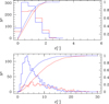 |
Fig. 6 Histogram distribution and cumulative distribution of FG (red) and SG (blue) RGB stars as a function of the radial distance r. Histograms and cumulative curves from r=0′ and r=3′ were obtained from the HST photometry (upper panel), while those from r∼2′ to r=30′ were obtained from the ground-based photometry (lower panel). We note that the x-scale is different for the two panels and that for the upper panel was extended to 6′ in order to improve the visualization. |
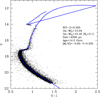 |
Fig. 7 V versus V-I CMD of the outer part of the cluster (r>15′). The blue line is the same best fitting isochrone shown in Figure 2. The parameters of the fitting are reported (see text for more details). |
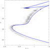 |
Fig. 8 Difference between the Hess diagrams of the full field photometry (see Figure 2) and the outer part (r>15′) photometry (see Figure 7). This diagram enhances the position of SG stars in the CMD. The best fitting isochrone from Figure 2 is reported as reference. |
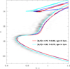 |
Fig. 9 Difference between the Hess diagrams of the full photometry (see Figure 2) and the outer part (r>15′) photometry (see Figure 7). The blue line is the same best fitting isochrone shown in Figure 2, while the red curved is the BASTI isochrone that bast matches the Padova isochrone. Cyan curve is the He-enhanced, [M/H]-poor BASTI isochrone that best reproduce the locus of SG stars. Parameters for the two BASTI isochrones are indicated. |
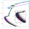 |
Fig. 10 Same as Figure 1, but with the best fitting Padova and BASTI isochrones for the FG and SG stars reported. Our targets are also reported (see text for more details). |
5 Second abundance determination
In the previous section, we found that the only way to properly interpret 47Tuc CMD is by using two isochrones having different parameters. Now we want to discuss the impact of this result on the parameter and abundance determination of our targets. Parameters for HB and SGB stars were obtained from the V-I color which is sensitive only to temperature, so nothing changes for them. For AGB stars we highlighted an intrinsic color spread due to the fact that they belong to FG and SG and to a differential mass-loss during the previous RGB phase. For this reason the best temperature estimation for them is the Teff versus V-I relation that can be obtained from the corresponding portion of the isochrone (see Figure 1) instead of the Teff versus V relation we used before. As far as RGB targets are concerned, FG and SG isochrones have a temperature difference of 55–65 K, with the SG isochrone being hotter. For this reason we just adjusted temperatures for RGB SG targets of +60K. The situation for MS targets is a bit more complex. The inset in Figure 10 shows that FG MS targets follow nicely the FG isochrone, with some outlier that can be explained by photometric errors. SG targets instead show a different behavior. A fraction of them follow closely the SG isochrone, while the other fraction appears to follow the FG isochrone. We investigate this weird behavior in Figure 11, where we plot only SG targets. In this figure we build the SG binary sequence (the yellow region) by adding to each SG isochrone point all the fainter points using the equation of Section 5 in Albornoz et al. (2021). We see clearly that the targets follow either the metal-poor SG isochrone or the metalrich FG isochrone. These last ones are indicated with magenta squares. Our explanation is that they are SG stars, but their redder position is due to the fact that they are in a binary system. So in the MS sample we have single FG stars and a mix of single and binary SG stars. The reason for that is probably the following. When Briley et al. (2004) selected the targets, they defined a mean ridge line for the cluster along the MS/TO/SGB region located likely in the middle of the two isochrones of Figure 11. Then they include in their sample only stars within a certain distance from this mean line, and by this criterion they included only single FG stars but both single and binary SG stars. In any case, in order to have the best temperature estimation possible, we have to treat single and binary SG stars in a different way. For FG targets we stay with the same Teff we obtained in Section 3. For single SG targets we modified the Teff we obtained in Section 3 by adding the mean temperature difference between the two isochones in their MS part, that is by adding +60K. For binary SG targets we just maintain the same Teff without any change. In the following discussion we check if this decision is the correct one. As far as gravity is concerned, we check that the best option was, for all the targets, to follow the same methodology explained in Section 3 without any change. Finally microturbulence was obtained using the Mott et al. (2020) relation and the new temperatures. We report these final parameters in Table 3.
At this point, it is worth to check our parameters. First of all we report in Figure 12 our temperatures as a function of the V-I color. We have to consider, however, that stars with higher gravities tend to have redder a V-I color for the same temperature. To correct for this effect we took a typical HB star as reference (Teff = 5000 K, log(g)=2.5) and calculated its synthetic spectrum. We calculated then two spectra with the same temperature but with log(g)=4.0 (typical of a SGB target) and log(g)=4.5 (typical of a MS target). We found corrections of −0.009 and −0.019 mag respectively. The two corrections were applied to the colors of MS and SGB targets in Figure 12. We can see that our targets define a nice and narrow sequence with a mean temperature spread around the polynomial fit of 22 K.
We finally report in Figure 13 temperature and gravities and compare them with the isochrone of Figure 2. We plotted also an isochrone from the same database but with a global metallic-ity 0.15 dex lower, as a reference. The spread around the first isochrone is due to the temperature corrections we discussed above, and the SG targets (which are 0.15 dex more metal poor that the FG) are well represented by the second isochrone at the MS and RGB level, where such corrections were applied. We conclude that no major internal systematic errors appears and that our parameters are consistent among all the evolutionary phases.
Another important issue to discuss is the internal errors on [C/Fe] and [N/Fe]. Uncertainties on Teff, log(g) and vt translate on errors in the abundance determination as well as the S/N of the data. In addition we have to consider that the C content we measure also is affected by the uncertainties on [N/Fe], and the same happens for N that is affect by uncertainties on [C/Fe]. In order to estimate internal errors on [C/Fe] and [N/Fe] we first have to estimate error on stellar parameters. From what we said before we can adopt 30K as a reasonable estimation for the internal error in temperature. Also, the isochrone fitting procedure suggests that 0.05 is a good value for the uncertainty on gravity, while for the microturbulence we adopt 0.05 km/s. At this point we selected one representative stars for each evolutionary phase and estimated new [C/Fe] and [N/Fe] by varying stellar parameters of the indicated amount one by one. The variation of the abundances is indicated in Table 4, Columns 2–5. Column 6 gives the total error due to stellar parameters and S/N calculated as the root-square of the sum of the squares of the previous 4 columns. We now can calculate the error on [C/Fe] due to the error on [N/Fe] (Column 7), and the error on [N/Fe] due to the error on [C/Fe] (Column 8). Finally, column 9 gives the total error calculated as the root-square of the sum of the squares of the previous 3 columns.
As we can see, the major contributors to the final errors are uncertainty on temperature and the S/N of the data. Also uncertainty on [C/Fe] has a significative impact on the final [N/Fe] abundance, while uncertainty on [N/Fe] does not affect [C/Fe]. Table 4 shows that we can assume 0.06 dex as the typical internal error for [C/Fe] and 0.10 dex as the typical internal error for [N/Fe].
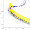 |
Fig. 11 Position on the CMD of our SG MS and SGB targets. Isochrones are those described in Figure 9. Targets highlighted by a magenta square are those considered as binaries (see text for more details). |
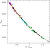 |
Fig. 12 Relation of Teff versus (V-I) obtained for our targets. The V-I color of MS and SGB stars was corrected for the gravity effect. The black line represents a 3rd degree polynomial fit (see text for more details). |
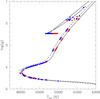 |
Fig. 13 Relation of log(g) versus Teff for our targets. The continuos black lines represents the isochrones we used to obtain the initial stellar parameters (see Fig. 2). The shaded black lines is an isochrone from the same database but with a global metallicity 0.15 dex lower. Red circles are FG targets, while blue circles are SG targets (see text for more details). |
6 Results
The new parameters were used to obtain the final abundances that are reported in Figures 14, 15 and Table 3. The main change with respect to Figure 4 is in the C abundances of single MS, SG targets. Now these abundances better overlap with those of the other MS targets and the MS’s star N versus C anticorrelation is significantly narrower. About the other targets, abundances did not change significantly.
In Figure 14, we report [N/Fe] versus [C/Fe], i.e. the N vs. C anticorrelation, together with the mean [C/Fe] and [N/Fe] values of each evolutionary phase with colored crosses surrounded by a black circles. These values are also reported in Table 5. Red crosses surrounded by red circles represent the mean C and N abundances for evolved FG and SG targets, i.e. the mean of the RGB/HB/AGB phases (see below for the reason why made this choice). We also reported the typical errors determined in the previous section. We can immediately see that the spread of the data is much larger than the typical error, making us confident that what we see in this figure is real. A value of [N/Fe]=+0.20 can be safely used to divide FG and SG targets as indicated by the dashed horizontal line of Figure 14 and this classification is reported in the Column 12 of Table 3. While the observed spread of FG stars is comparable with the typical error, the spread of SG stars is much bigger. We can infer then that FG stars have an homogeneous C and N content, while SG stars have a real intrinsic C and N spread.
As far as FG is concerned, we see that [C/Fe] decreases of ∼0.14 dex moving from the MS to the later phases, while [N/Fe] decreases of 0.10 dex. For SG instead, [C/Fe] and [N/Fe] have the same value for MS and SGB, then [C/Fe] decreases of ∼0.21 dex moving to later phases, while [N/Fe] decreases of 0.12 dex. These trends are indicated by the blue arrows. The behavior of FG and SG SGB stars are discussed further in the next paragraph. We can also see that SG targets suspected to be binaries (the magenta circles surrounded by thick black circles) follow nicely the trend defined by non-binary targets, suggesting that no systematic shift is introduced by the methodology we adopted above in order to obtain the final atmospheric parameters.
There are a couple of mismatches that we have to underline. The first concerns those N-rich SGB stars with [N/Fe]>1.0. These targets have N abundances slightly higher than their MS SG counterparts. This is hardly an evolutionary effect and it could be due to some residual systematic error on the determination of the N content. In any case this does not affect the following discussion. The second concerns the N versus C anticorrelation of RGB stars. While the FG RGB targets are well mixed with FG HBs and AGBs, the SG RGBs have a slightly higher C and N content compared to SG HBs and AGBs. This could be an evolutionary effect where, at the level of the RGB, the transition from MS to HB/AGB abundances is already completed for the FG, while it is still an ongoing process for the SG. Nevertheless, we treat the RGB, HB and ABG phases all together.
The inset in Figure 14 shows the mean ridge lines for the N vs. C anticorrelations of MS (magenta), SGB (yellow) and evolved (green) targets. While anticorrelations for MS and evolved targets are well detached, that of the SGB targets matches the FG part of the evolved anticorrelation, and then it moves gradually to match the SG MS anticorrelation. This behavior is due to two reasons. In the first place, during the SGB phase, stars change their superficial [C/Fe] and [N/Fe] abundances due to the first dredge-up, as we discuss below. We call the SGB region where this effect takes place “Abundance Changing Region” (ACR). The other reason is due to selection effects. Infact, FG SGB targets and the most N-poor of the SG SGB targets are located after the ACR (as we will show later) and so they follow the evolved anticorrelation. On the other hand, the most N-rich of the SG SGB targets are located before this region and so they follow the MS anticorrelation.
Another thing we have to notice in Figure 14 is that, while the mean FG SGB [C/Fe] abundance matches that of the FG evolved stars, the [N/Fe] abundances for the same group is higher instead. This is because the most N-poor FG SGB star are missed from the sample (i.e., there are very few yellow targets with [N/Fe]<0.0 in Figure 14), very likely due to selection effects. On the other hand the SGB SGB population is well represented and its mean [C/Fe] and [N/Fe] abundances match those of the SG MS stars.
Figure 14 also shows that, if we compare HB targets (cyan) with the RGB (green) and the AGB (black), a tail of C-poor stars is missing. The explanation for this behavior is that, while we observe the entire HB and so we mapped the entire N versus C anticorrelation down to the lowest C abundance, for the RGB and the AGB we missed the most extremes targets, i.e. the most C-poor. In fact, these targets should be the bluest and we cut them off during the selection process. If we look carefully Figure 10, we see actually that on the blue side of our RGB and AGB targets there are several stars (all members) and we can guess that those would populate the very C-poor tail of the N versus C anticorrelation. The missing targets belong to the SG, as also clearly visible in Figure 14. On the other hand Figure 14 shows that SG RGB and AGB targets map better the anticorrelation for evolved stars between [N/Fe]=+0.20 and [N/Fe]=+0.50. So the best estimation for the mean C and N abundances of the evolved SG targets is the mean of the abundances of the SG RGB/HB/AGB phases. We adopted the same procedure to calculate the mean abundances of the FG evolved targets. These values are those reported as red symbols in Figure 14 and is used in the following discussion.
Figure 15 shows the trend of [C/Fe] and [N/Fe] with the evolutionary phase, that is represented by the distance (in magnitudes) along the isochrone from a MS reference point and the projection of each target onto the isochrone. In order to calculate the distance, we followed this procedure:
Since the points of the isochrone are not evenly spaced, we interpolated it with a 0.01 mag. step.
Then we associated to each target the closest interpolated point.
Choosing the point closest to the faintest target (the MS star with V=20 in Figure 2) as reference, we calculated the distance of each point along the isochrone path.
We did not consider the jump from the RGB-tip to the zeroage HB in our calculation, so the point at the RGB-tip and the following at the zero-age HB have the same distance.
For this procedure we used the isochrone from the Padova database (the blue line in Figures 10 and 2).
For each sub-population (MS, SGB, RGB, HB and AGB) we divided the targets in FG and SG groups. For each of them we then calculated the mean [C/Fe] and [N/Fe] abundances (the same reported in Table 5) and the mean distance. The mean values are reported as big black circles with inside a cross of the color of the sub-population.
In Figure 15, the mean abundance trends are indicated by black lines, each one named with the population they represent (FG or SG). As far as FG is concern, MS stars have the mean [C/Fe] abundance of –0.02 dex, that we assume remains constant until the ACR (we have too few FG SGB targets before this region to be certain). After this region the SGB mean FG C abundance decrease to –0.16 dex and stays constant until the AGB. For the SG instead, MS stars have the mean [C/Fe] abundance of –0.24 dex that stays constant until the ACR. In this case, a significant fraction of our targets lie before this region so we can be certain. Then it decreases to a value of about –0.45 dex and remains constant. The lower panel shows that also N abundances does have the same behavior, but with a much smaller decrease of –0.10 dex for the FG, and –0.12 dex for the SG. We can also say that we find no abundance variation at the RGB-bump level, that have log(g)~2.5 (Dist.=5.5).
A decrease of ~-0.15÷-0.20 dex in C after the ACR is compatible with the effect of the first dredge-up. Vincenzo et al. (2021) performed a test of theoretical stellar models that predicts a C-depletion of –0.14 dex after the first dredge-up, very close to the value we find. However, the same models predict a N enhancement of +0.19 dex, while we find a N depletion of ~-0.10÷-0.12 dex. On the other hand (Salaris et al. 2020, see their figure 1) predicts that, for an old population (13 Gyr), the ∆[N/Fe] expected is of the order of about –0.1 dex, close to the value we obtain. In any case the first dredge-up appear to the cause of the C and N behavior we find at the level of the ACR.
Figures 14 and 15 show a clear decrease in carbon an nitrogen when stars move away from the MS, that is complete (or almost complete) at the RGB level, at least for V<16.0. We want to investigate if we can exactly identify the region of the SGB were this decrease happens, that we previously called the abundance changing region (i.e., ACR). For this purpose we plot in Figure 16 the SGB region (upper panel) with FG SGB targets in red and SG SGB targets in blue. In the middle panel we report in the X-axis the distance parameters of the targets from the reference point (see above for the definition) and in the Y axis a parameter we call ∆(CNMS anticorrelation). This parameter is the ∆[C/Fe] difference between the target [C/Fe] and the point of the MS anticorrelation (the magenta line in the inset of Figure 14) closest to that target. For this purpose we interpolated the MS anticorrelation with a 0.01 dex step. This panel shows clearly that both subpopulation show the same behavior with the ∆(CNMS anticorrelation) parameters that starts to decrease at Dist.=2.82, with the decrease being complete for Dist.=2.93. These two limits are indicated by the two green lines. This region can be transformed back to the CMD and is the SGB part between the two green lines of the upper panel of Figure 16 (between V-I=0.77 and V-I=0.85). The cause of this transition is very likely the first dredge-up as we discussed before. In the same figure (bottom panel), we report also the [Fe/H] abundance of stars from Marino et al. (2016) (we do not have iron abundance for the other targets) and we see that iron abundance does not vary along the SGB. So we can safely assume that the drop in C and N is not accompanied by a drop in iron and that the variation in [C/Fe] and [N/Fe] are not due to a variation in [Fe/H]. The mean [Fe/H] for these stars is −0.73±0.01, very close to the value we assumed for all the targets ([Fe/H]=–0.70).
We see also that almost all the FG SGB stars are located at the very end of the ACR, when both C and N abundances reach their minimum value, while at least half of the SG SGB stars are located on the left side still keeping their MS C and N content. This can explain the weird behavior of the C versus N anticorrelation of SGB targets visible in Figure 14. Most of those that belong to the FG already suffered a decrease in C and N, so their trend matches that of the more evolved phases. On the other hand many of those that belong to the SG still retain their original MS C and N content and so their trend matches that of the MS. This is confirmed by the blue circles surrounded by green squares in Figure 16 (middle panel). These are the SG SGB target with [N/Fe] in the range 0.20÷0.50 dex and that in Figure 14 are the SG SGB targets that are on average the ones that most moved away from the mean MS anticorrelation. As expected, also these target are located toward the end of the ACR and they moved away from the MS trend because that already experimented the C and N abundance decrease.
Another question rises at this point, namely why almost all FG SGB targets are located in the very red part of the SGB, while the SG SGB targets are spread all over. It hard to give an answer but a possible explanation is that FG SGB stars follow a different path along this CMD region (Anderson et al. 2009 found a split here) and they were missed due to selection effects. Also, if we look carefully at Figure 14, we see that FG SGB targets are almost all located at higher N abundances ([N/Fe]>0.0) compared to their evolved counterparts (RGB, HB and AGB) and that there is just 1 FG SGB star with a low N content ([N/Fe]= –0.20). This reinforces the idea that the low N-content FG SGB stars were completely missed during the target selection because they are located in a different part of the CMD, very likely at lower V magnitudes. Future investigations will clarify this point.
Errors on the abundance determination.
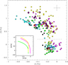 |
Fig. 14 Final [N/Fe] vs [C/Fe] anticorrelation we obtained for our targets. Magenta, yellow, green, cyan, and black symbols represents MS, SGB, RGB, HB, and AGB targets, respectively. Mean values for FG and SG stars are indicated with crosses surrounded by black circles. The horizontal line at [N/Fe]=+0.20 divides FG from SG targets. The inset shown the mean ridge lines for the N versus C anticorrelations of MS (magenta), SGB (yellow) and evolved (green) targets. Error-bar shows the typical errors (see text for more details). |
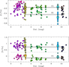 |
Fig. 15 Plots of [C/Fe] versus Dist. (upper panel) and [N/Fe] versus Dist. (lower panel) for our targets. Magenta, yellow, green, cyan, and black symbols represents MS, SGB, RGB, HB, and AGB targets, respectively. The targets have a red or blue circle inside if they belong to the FG or SG respectively. Mean values for FG and SG stars at the different phases are indicated with crosses surrounded by big black circles. The horizontal line at [N/Fe]=+0.20 divides FG from SG targets, while the continuous black lines represent the mean values of unevolved (before the SGB) and evolved (after the SGB) stars (see text for more details). |
Mean [C/Fe] and [N/Fe] abundances for FG and SG for the different evolutionary phases.
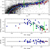 |
Fig. 16 Upper panel: distribution on the CMD of FG (red) and SG (blue) SGB targets. The SGB region where abundance change happens is indicated by the two green lines. Middle panel: abundance variation along the SGB. The y coordinate is the [C/Fe] difference between each target and the point of the MS anticorrelation (the magenta line in the inset of Figure 14) closest to that target. Bottom panel: [Fe/H] as a function of the position along the SGB. See text for more details. |
7 Conclusions
In this paper, we have analyzed the V vs V-I CMD of the globular cluster NGC 104 in the inner part and out to 25′ from the center. We also analyzed a sample of low, medium, and high resolution spectra covering CH and CN blue and UV bands in order to obtain [C/Fe] and [N/Fe] abundances for a sample of targets covering all the evolutionary phases, from the MS to the AGB. Our findings are as follows:
Spectroscopic targets define a [N/Fe] versus [C/Fe] anticorrelation where FG and SG stars can be easily separated.
In the CMD, FG and SG targets define two distinct sequences that can be traced from the MS to the AGB.
The SG is more centrally concentrated while the FG dominates beyond 15′.
In order to properly fit the CMD, two isochrones are required.
The FG CMD can be fit with an isochrone having E(V-I)=0.025, (m-M)V=13.24, [M/H]=–0.70, Y=0.25 and Age=13.0 Gyrs.
The SG CMD can be fit with an isochrone having the same reddening and distance modulus, but with [M/H]=–0.85, Y=0.275. An older age of 14.0 Gyrs is also required to match the SG TO color.
By consequence, the SG is more metal-poor, He-richer and possibly older than the FG.
Both C and N decrease moving away from the MS. The decrease in C is more significant (–0.14 for FG and –0.21 for SG), while for N is of the order of 0.10 dex.
This abundance decrease happens at the level of the SGB, between V-I=0.77 and V-I=0.85 and it is very likely connected with the first dredge-up, both for the location where it occurs and for the amount of the decrease.
The decrease in C and N is not accompanied by a drop in [Fe/H], that is constant along the SGB.
We finally want to underline the fact that, when stars with different C and N abundances occupy distinct regions even in the well-behaved V vs. V-I diagram, a proper CMD fitting in any GC CMD will likely require at least two isochrones with differing helium content, metallicity, and possibly age. In this sense, previous parameters determinations may benefit from a revision, even if in many cases changes could result minor.
Data availability
Full Table 3 is available at the CDS via https://cdsarc.cds.unistra.fr/viz-bin/cat/J/A+A/700/A213
Acknowledgements
S.V. gratefully acknowledges the support provided by Fonde-cyt Regular no. 1220264 and by the ANID BASAL project FB210003. L.M. gratefully acknowledges support from ANID-FONDECYT Regular Project no. 1251809. The authors acknowledge the anonymous referee for the contruc-tive report. This work has made use of data from the European Space Agency (ESA) mission Gaia (https://www.cosmos.esa.int/gaia), processed by the Gaia Data Processing and Analysis Consortium (DPAC, https://www.cosmos.esa.int/web/gaia/dpac/consortium). Funding for the DPAC has been provided by national institutions, in particular the institutions participating in the Gaia Multilateral Agreement.
References
- Albornoz, A., Villanova, S., Cortes, C. C., Ahumada, J. A., & Parisi, C. 2021, AJ, 161, 76 [NASA ADS] [CrossRef] [Google Scholar]
- Alonso, A., Arribas, S., & Martinez-Roger, C. 1999, A&AS, 140, 261 [CrossRef] [EDP Sciences] [Google Scholar]
- Anderson, J., Piotto, G., King, I. R., Bedin, L. R., & Guhathakurta, P. 2009, ApJ, 697, 58 [Google Scholar]
- Bastian, N., Lamers, H. J. G. L. M., de Mink, et al. 2013, MNRAS, 436, 2398 [CrossRef] [Google Scholar]
- Baumgardt, H., & Hilker, M. 2018, MNRAS, 478, 1520 [Google Scholar]
- Bressan, A., Marigo, P., Girardi, L., et al. 2012, MNRAS, 427, 127 [NASA ADS] [CrossRef] [Google Scholar]
- Briley, M. 1997, AJ, 114, 1051 [Google Scholar]
- Briley, M., Harbeck, D., Smith, G. H., & Grebel, E.K. 2004, AJ, 127, 1588 [Google Scholar]
- Carretta, E., Bragaglia, A., Gratton, R. G., et al. 2009, A&A, 505, 117 [NASA ADS] [CrossRef] [EDP Sciences] [Google Scholar]
- Carretta, E., Bragaglia, A., Gratton, R. G., et al. 2010, A&A, 520, A95 [NASA ADS] [CrossRef] [EDP Sciences] [Google Scholar]
- Cohen, J. G., Kirby, E. N., Simon, J. D., & Geha, M. 2010, ApJ, 725, 288 [Google Scholar]
- D’Antona, F., Vesperini, E., D’Ercole, A., et al. 2016, MNRAS, 458, 2122 [Google Scholar]
- Decressin, T., Meynet, G., Charbonnel, C., Prantzos, N., & Ekstrom, S. 2007, A&A, 464, 1029 [NASA ADS] [CrossRef] [EDP Sciences] [Google Scholar]
- de Mink, S. E., Pols, O. R., Langer, N., & Izzard, R. G. 2009, A&A, 507, L1 [NASA ADS] [CrossRef] [EDP Sciences] [Google Scholar]
- Gaia Collaboration (Prusti, T., et al.) 2016, A&A, 595, A1 [NASA ADS] [CrossRef] [EDP Sciences] [Google Scholar]
- Gaia Collaboration (Vallenari, A., et al.) 2023, A&A, 674, A1 [NASA ADS] [CrossRef] [EDP Sciences] [Google Scholar]
- Geisler, D., Villanova, S., O’Connell, J. E., et al. 2021, A&A, 652, A157 [NASA ADS] [CrossRef] [EDP Sciences] [Google Scholar]
- Harbeck, D., Grebel, E. K., & Smith, G. H. 2004, AJ, 125, 197 [Google Scholar]
- Harris, W. E. 1996, AJ, 112, 1487 [Google Scholar]
- Kurucz, R. L. 1970, SAO Special Report 309 [Google Scholar]
- Majewski, S. R., Schiavon, R. P., Frinchaboy, P. M., et al. 2017, AJ, 154, 94 [NASA ADS] [CrossRef] [Google Scholar]
- Marin-Franch, A., Aparicio, A., Piotto, G., et al. 2009, ApJ, 694, 1498 [Google Scholar]
- Marino, A. F., Milone, A. P., Piotto, G., et al. 2009, A&A, 505, 1099 [CrossRef] [EDP Sciences] [Google Scholar]
- Marino, A. F., Milone, A. P., Casagrande, L., et al. 2016, MNRAS, 459, 610 [NASA ADS] [CrossRef] [Google Scholar]
- Massari, D., Mucciarelli, A., Ferraro, F. R., et al. 2014, ApJ, 795, 22 [NASA ADS] [CrossRef] [Google Scholar]
- Milone, A. P., Bedin, L. R., Piotto, G., et al. 2008, ApJ, 673, 241 [NASA ADS] [CrossRef] [Google Scholar]
- Milone, A. P., Piotto, G., Bedin, L. R., et al. 2012, ApJ, 744, 58 [NASA ADS] [CrossRef] [Google Scholar]
- Milone, A. P., Piotto, G., Renzini, A., et al. 2017, MNRAS, 464, 3636 [Google Scholar]
- Moro, D., & Munari, U. 2000, A&AS, 147, 361 [NASA ADS] [CrossRef] [EDP Sciences] [Google Scholar]
- Mott, A., Steffen, M., Caffau, E., & Strassmeier, K. G. 2020, A&A, 638, A58 [EDP Sciences] [Google Scholar]
- Nardiello, D., Libralato, M., Piotto, G., et al. 2018, MNRAS, 481, 3382 [NASA ADS] [CrossRef] [Google Scholar]
- Norris, J., & Freeman, K. C. 1982, ApJ, 254, 143 [Google Scholar]
- Pancino, E., Romano, D., Tang, B., et al. 2017, A&A, 601, A112 [NASA ADS] [CrossRef] [EDP Sciences] [Google Scholar]
- Pancino, E., Zocchi, A., Rainer, M., et al. 2024, A&A, 686, A283 [NASA ADS] [CrossRef] [EDP Sciences] [Google Scholar]
- Pietrinferni, A., Hidalgo, S., Cassisi, S., et al. 2021, ApJ, 908, 102 [NASA ADS] [CrossRef] [Google Scholar]
- Piotto, G., Bedin, L. R., Anderson, J., et al. 2007, ApJ, 661, 53 [Google Scholar]
- Piotto, G., Milone, A. P., Bedin, L. R., et al. 2015, AJ, 149, 91 [Google Scholar]
- Renzini, A., D’Antona, F., Cassisi, S., et al. 2015, MNRAS, 454, 4197 [Google Scholar]
- Salaris, M., Cassisi, S., & Pietrinferni, A. 2016, A&A, 590, A64 [CrossRef] [EDP Sciences] [Google Scholar]
- Salaris, M., Usher, C., Martocchia, S., et al. 2020, MNRAS, 492, 3459 [Google Scholar]
- Stetson, P. B., Pancino, E., Zocchi, A., Sanna, N., & Monelli, M. 2019, MNRAS, 485, 3042 [Google Scholar]
- Villanova, S., Geisler, D., Carraro, G., et al. 2013, ApJ, 778, 186 [Google Scholar]
- Villanova, S., Geisler, D., Gratton, R. G., & Cassisi, S. 2014, ApJ, 791, 107 [Google Scholar]
- Vincenzo, F., Weinberg, D. H., Montalbán, J., et al. 2021, arXiv e-prints [arXiv:2106.03912] [Google Scholar]
All Tables
Mean [C/Fe] and [N/Fe] abundances for FG and SG for the different evolutionary phases.
All Figures
|
Fig. 1 Distribution of NGC 104 member stars in the sky. Blue and red points are stars from ground-based photometry, while black points in the center are stars from the HST Large Legacy Treasury Program. The radial cut at 15′ was used to separate the inner from the outer cluster region. Black circles with colored insets represent MS (magenta), SGB (yellow), RGB (green), HB (cyan) and AGB (black) targets (see text for more details). |
| In the text | |
|
Fig. 2 Position on the CMD of our targets. The blue and yellow line is the best fitting isochrone we used for the parameter determination. Blue and red symbols inside each circle represent FG and SG stars respectively (see text for more details). |
| In the text | |
|
Fig. 3 Example of spectrosynthesis. Panels on the left show the synthesis for C while panels on the right show the synthesis for N. The upper row shows the synthesis for the MS target #1_13, the middle row shows synthesis for the HB target #RHB_I_a_40848, and the lower row shows the synthesis for the SGB target N104e_51104. The wavelength range used for the abundance determination is shown as a shaded region. Observed spectra are in green. Red spectra show the best match, while blue and black spectra represent abundance variations of ±0.5 dex for C respectively, while for N we used ±1.0 dex for low resolution spectra of MS and SGB stars (upper panel) and ±0.5 dex for intermediate and high resolution spectra of SGB, RGB, HB and AGB stars (middle and lower panel). |
| In the text | |
|
Fig. 4 [N/Fe] versus [C/Fe] anticorrelation as obtained from the first abundance determination run. The red line divides MS targets on the right from RGB/HB/AGB targets on the left. SGB targets are located on both sides of the red line. The black line divides FG from SG stars. Red arrows indicate stars for which Marino et al. (2016) gives no [N/Fe]. For these stars we assumed [N/Fe]=0.0 as an upper limit (see text for more details). |
| In the text | |
|
Fig. 5 Ground-based (left) and HST (right) CMDs of the cluster. FG generation (red) and SG (blue) star selection is indicated. The green line is the isochrone used for this selection (see text for more details). |
| In the text | |
|
Fig. 6 Histogram distribution and cumulative distribution of FG (red) and SG (blue) RGB stars as a function of the radial distance r. Histograms and cumulative curves from r=0′ and r=3′ were obtained from the HST photometry (upper panel), while those from r∼2′ to r=30′ were obtained from the ground-based photometry (lower panel). We note that the x-scale is different for the two panels and that for the upper panel was extended to 6′ in order to improve the visualization. |
| In the text | |
|
Fig. 7 V versus V-I CMD of the outer part of the cluster (r>15′). The blue line is the same best fitting isochrone shown in Figure 2. The parameters of the fitting are reported (see text for more details). |
| In the text | |
|
Fig. 8 Difference between the Hess diagrams of the full field photometry (see Figure 2) and the outer part (r>15′) photometry (see Figure 7). This diagram enhances the position of SG stars in the CMD. The best fitting isochrone from Figure 2 is reported as reference. |
| In the text | |
|
Fig. 9 Difference between the Hess diagrams of the full photometry (see Figure 2) and the outer part (r>15′) photometry (see Figure 7). The blue line is the same best fitting isochrone shown in Figure 2, while the red curved is the BASTI isochrone that bast matches the Padova isochrone. Cyan curve is the He-enhanced, [M/H]-poor BASTI isochrone that best reproduce the locus of SG stars. Parameters for the two BASTI isochrones are indicated. |
| In the text | |
|
Fig. 10 Same as Figure 1, but with the best fitting Padova and BASTI isochrones for the FG and SG stars reported. Our targets are also reported (see text for more details). |
| In the text | |
|
Fig. 11 Position on the CMD of our SG MS and SGB targets. Isochrones are those described in Figure 9. Targets highlighted by a magenta square are those considered as binaries (see text for more details). |
| In the text | |
|
Fig. 12 Relation of Teff versus (V-I) obtained for our targets. The V-I color of MS and SGB stars was corrected for the gravity effect. The black line represents a 3rd degree polynomial fit (see text for more details). |
| In the text | |
|
Fig. 13 Relation of log(g) versus Teff for our targets. The continuos black lines represents the isochrones we used to obtain the initial stellar parameters (see Fig. 2). The shaded black lines is an isochrone from the same database but with a global metallicity 0.15 dex lower. Red circles are FG targets, while blue circles are SG targets (see text for more details). |
| In the text | |
|
Fig. 14 Final [N/Fe] vs [C/Fe] anticorrelation we obtained for our targets. Magenta, yellow, green, cyan, and black symbols represents MS, SGB, RGB, HB, and AGB targets, respectively. Mean values for FG and SG stars are indicated with crosses surrounded by black circles. The horizontal line at [N/Fe]=+0.20 divides FG from SG targets. The inset shown the mean ridge lines for the N versus C anticorrelations of MS (magenta), SGB (yellow) and evolved (green) targets. Error-bar shows the typical errors (see text for more details). |
| In the text | |
|
Fig. 15 Plots of [C/Fe] versus Dist. (upper panel) and [N/Fe] versus Dist. (lower panel) for our targets. Magenta, yellow, green, cyan, and black symbols represents MS, SGB, RGB, HB, and AGB targets, respectively. The targets have a red or blue circle inside if they belong to the FG or SG respectively. Mean values for FG and SG stars at the different phases are indicated with crosses surrounded by big black circles. The horizontal line at [N/Fe]=+0.20 divides FG from SG targets, while the continuous black lines represent the mean values of unevolved (before the SGB) and evolved (after the SGB) stars (see text for more details). |
| In the text | |
|
Fig. 16 Upper panel: distribution on the CMD of FG (red) and SG (blue) SGB targets. The SGB region where abundance change happens is indicated by the two green lines. Middle panel: abundance variation along the SGB. The y coordinate is the [C/Fe] difference between each target and the point of the MS anticorrelation (the magenta line in the inset of Figure 14) closest to that target. Bottom panel: [Fe/H] as a function of the position along the SGB. See text for more details. |
| In the text | |
Current usage metrics show cumulative count of Article Views (full-text article views including HTML views, PDF and ePub downloads, according to the available data) and Abstracts Views on Vision4Press platform.
Data correspond to usage on the plateform after 2015. The current usage metrics is available 48-96 hours after online publication and is updated daily on week days.
Initial download of the metrics may take a while.