| Issue |
A&A
Volume 700, August 2025
|
|
|---|---|---|
| Article Number | A224 | |
| Number of page(s) | 15 | |
| Section | Planets, planetary systems, and small bodies | |
| DOI | https://doi.org/10.1051/0004-6361/202555787 | |
| Published online | 22 August 2025 | |
Giant planet formation via pebble accretion across different stellar masses
1
Department of Earth, Environmental and Planetary Sciences,
6100 Main MS 126, Rice University,
Houston,
TX
77005,
USA
2
Department of Astrophysics, University of Zurich,
Winterthurerstrasse 190,
8057
Zurich,
Switzerland
★ Corresponding author: This email address is being protected from spambots. You need JavaScript enabled to view it.
Received:
3
June
2025
Accepted:
30
June
2025
Abstract
Aims. The occurrence rate of cold Jupiters, giant planets orbiting in the outer orbital region (≳1 au), was found to depend on stellar mass. The formation environment in the protoplanetary disks, which depends on the mass of the host star, regulates core formation and the subsequent gas accretion. In this study, we simulate giant planet formation via pebble accretion accounting for various stellar masses, core formation times, disk turbulent viscosities, and grain opacities.
Methods. We use a self-consistent formation model that calculates the solid accretion rate and gas accretion rate of growing protoplanets. We investigate how the planetary formation, in particular, the contraction of the envelope, and the formation timescale change under different conditions.
Results. We find that to reproduce the observed occurrence rate of cold Jupiters, giant planets must undergo slow envelope contraction after they reach pebble isolation, which lasts for several Myrs. Such a slow contraction phase can be achieved when the grain opacity is assumed to be as high as that of the interstellar medium (ISM). If the grain opacity is smaller than the ISM opacity by a factor of ten or more, the growing protoplanets reach crossover mass within 3 Myrs and form too many cold Jupiters around stars of ≳0.4 M⊙. Protoplanets around low-mass stars <0.4 M⊙ take ≳10 Myrs to reach crossover mass also with low grain opacity. If the grain opacity in the planetary envelope is much lower than that of ISM, other mechanisms, such as atmospheric recycling or planetesimal accretion, is required for cold Jupiter formation. We next explore how the deposition of the accreted heavy elements to the planetary envelope changes the formation timescale. Our model suggests that the formation timescale could be longer due to heavy-element enrichment, resulting from the lower core mass at pebble isolation. We conclude that the details of the formation processes have a significant effect on the planetary growth and therefore, the formation of gaseous planets.
Key words: planets and satellites: formation / planets and satellites: gaseous planets / protoplanetary disks
© The Authors 2025
 Open Access article, published by EDP Sciences, under the terms of the Creative Commons Attribution License (https://creativecommons.org/licenses/by/4.0), which permits unrestricted use, distribution, and reproduction in any medium, provided the original work is properly cited.
This article is published in open access under the Subscribe to Open model. This email address is being protected from spambots. You need JavaScript enabled to view it. to support open access publication.
1 Introduction
Cold Jupiters are massive gaseous planets, usually categorized as those heavier than Neptune (≳30 M⊕) that orbit their host star beyond the inferred ice lines (≳1 au). The occurrence rate of cold Jupiters is usually constrained with RV observations (Johnson et al. 2009; Montet et al. 2014; Rosenthal et al. 2021; Fulton et al. 2021; Hirsch et al. 2021; Ribas et al. 2023; Bonomo et al. 2023; Pass et al. 2023). The observational data suggest that cold Jupiters are more common around more massive stars with higher metallicity. While the occurrence rate of cold Jupiters is constrained around 20% around G-type stars, it decreases lower than 10% around M- and K-type stars (Fulton et al. 2021). The occurrence rate is rather low (less than 1.5%) around the low-mass (0.1-0.3 M⊙) M dwarfs (Pass et al. 2023), but two confirmed planets, LHS 252 b (Morales et al. 2019) and GJ 83.1 b (Feng et al. 2020; Quirrenbach et al. 2022), and several candidates are detected there.
This result has been interpreted as a confirmation of the core accretion model (e.g. Mizuno 1980) since the solid material required for forming heavy-element cores is more abundant around those stars. In the core formation scenario, planetesimal and/or pebble accretion form a massive solid core (∼10 M⊕). The solid core accretes surrounding disk gas and forms a gaseous envelope around the core. Once the protoplanet reaches the crossover mass, where the envelope mass equals the solid core mass, the protoplanet starts a rapid gas accretion (Pollack et al. 1996; Ikoma et al. 2000). The crossover mass is usually considered the starting point of runaway gas accretion. To form gas giant planets, protoplanets must reach the crossover mass before the disk dissipation. In the core accretion model, the occurrence rate of giant planets depends on the timescales of core formation and the subsequent gas accretion. Besides the core accretion model, the gravitational instability scenario (Boss 2006, 2019) is also suggested to form giant planets around low-mass M dwarfs (Morales et al. 2019). However, the relation between the occurrence rate and the stellar metallicity is not explained in this formation mechanism (Mercer & Stamatellos 2020). Therefore, the core accretion model would be the primary formation mechanism of cold Jupiters, while some of the giant planets around lower mass stars might be formed via gravitational instability.
Various formation models investigated how the occurrence rate of giant planets changes with the assumed stellar properties. The planetesimal accretion scenario is the classical formation model for a massive solid core (Inaba et al. 2003; Kobayashi & Tanaka 2021, 2023). Population synthesis models based on the planetesimal accretion scenario (Ida & Lin 2005; Alibert et al. 2011; Miguel et al. 2019; Burn et al. 2021; Guo et al. 2025) show that the formation rate of giant planets increases with stellar mass, which is consistent with the observations. However, the planetesimal accretion scenario has difficulty in the formation of giant planets around M dwarfs since the current planetesimal accretion model failed to form a massive solid core (Miguel et al. 2019; Schlecker et al. 2022).
In the pebble accretion scenario, protoplanets grow via accretion of small millimeter-to-centimeter-sized solids. Since the available pebble flux increases with the stellar metallicity and disk mass, Liu et al. (2019) found that giant planet formation is more efficient around higher mass stars with higher metal-licity. The solid core growth stops at the pebble isolation mass (Lambrechts et al. 2014; Bitsch et al. 2018), where pebbles are stalled from drifting inward at the pressure bump formed by the protoplanet. Since the pebble isolation mass is smaller around lower mass stars, the formation of solid cores that are massive enough to trigger runaway gas accretion is less efficient around lower mass stars (Liu et al. 2019, 2020). To form giant planets around lower mass stars, the pebble accretion scenario requires multiple planet formation and giant impacts between them to grow further than the pebble isolation mass (Pan et al. 2024, 2025).
The pebble accretion models successfully reproduced the observed trend in the occurrence rate of giant exoplanets. However, these studies mainly focus on the formation of solid cores, and many simplifications are used for the gas accretion process. Figure 1 shows our disk model at t = 0.1 Myrs. In the above pebble accretion models, protoplanets are assumed to start the Kelvin-Helmholtz contraction once the protoplanet reaches the pebble isolation mass. The Kelvin-Helmholtz contraction timescale depends on the boundary conditions of the planetary envelope (Piso & Youdin 2014) and the grain opacity (Ikoma et al. 2000), which strongly affects the giant planet formation (Bitsch & Savvidou 2021). Previous studies have used the fixed grain opacity and neglected the effects of boundary conditions. Therefore, it is still unclear how these parameters affect the formation of cold Jupiters, especially in the pebble accretion scenario.
Alibert et al. (2011) pointed out that the formation rate of giant planets is related to the disk’s lifetime since the protoplanets must undergo rapid gas accretion before disk dissipation. Despite the observations showing a large variety in the disk’s lifetime (Bayo et al. 2012; Ribas et al. 2015; Richert et al. 2018), how the occurrence rate of giant planets changes with the disk lifetime is not well discussed. While the detection of the inner dust ring in circumstellar disks shows that the disk’s lifetime rarely depends on the stellar mass (Richert et al. 2018), theoretical models for X-ray photoevaporation predict that the disk lifetime is longer around the lower mass stars because of the weaker X-ray irradiation (Picogna et al. 2021). Additionally, long-lived accretion disks are detected around M-type stars, known as Peter Pan disks (Silverberg et al. 2020). If the disk lifetime is longer around the lower mass stars, the giant planets may form in the core accretion scenario around M-dwarfs, even if the available solids are less abundant.
In this work, we model giant planet formation via pebble accretion while focusing on the crossover time, which is the time it takes for a protoplanet to reach the crossover mass. We investigate how the crossover time changes with the formation environment and how the occurrence rate changes with stellar type. In Sect. 2, we describe our formation model. In Sect. 3, we present the results of our numerical model and show how the crossover time changes with the formation environment. We discuss our results and model in Sect. 4. Our summary and conclusions are presented in Sect. 5.
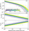 |
Fig. 1 Disk model used in this work. Panels a–c show the surface density of the gaseous disk, disk temperature, and the disk’s aspect ratio around different stellar masses as shown in the color bar in panel a. The horizontal dashed line in panel b shows Tdisk = 170 K, where H2O condenses. Here, we show the case when t = 105 yr. |
2 Methods
2.1 Disk model
Our disk model is based on the self-similar solution for the surface density profile of a gaseous disk (Lynden-Bell & Pringle 1974). We assume that the heating of the disk’s mid-plane gas is dominated by irradiation from the central star rather than viscous heating, where cold Jupiters form. Assuming a vertically optically thin and radially optically thick disk, the mid-plane temperature, Tdisk, is given by (e.g., Chiang & Goldreich 1997; Ida et al. 2016)
 (1)
(1)
where Ls and Ms are the luminosity and mass of central star, and r is the radial distance from the central star. If the disk viscosity scales with the radial distance as ν ∝ rγ, the surface density of disk gas, Σgas, is given as
 (2)
(2)
with
 (3)
(3)
 (4)
(4)
 (5)
where Mdisk,0 is the disk total mass at t = 0, Rdisk is a radial scaling length of the disk, τvis is the characteristic viscous timescale, and νd is a disk gas viscosity at r = Rd. We use the α-viscosity model (Shakura & Sunyaev 1973) and the disk gas viscosity is written as νd = αacch2gasΩK, where αacc is the viscosity parameter, hgas is the disk’s scale height, and ΩK is the orbital angular velocity. The disk’s scale height is expressed as hgas = cs/ΩK, where cs is the sound speed of the disk gas. The sound speed is obtained using the ideal gas law, assuming a mean molecular weight of 2.34. In this work, we use the fixed αacc = 10−3.
(5)
where Mdisk,0 is the disk total mass at t = 0, Rdisk is a radial scaling length of the disk, τvis is the characteristic viscous timescale, and νd is a disk gas viscosity at r = Rd. We use the α-viscosity model (Shakura & Sunyaev 1973) and the disk gas viscosity is written as νd = αacch2gasΩK, where αacc is the viscosity parameter, hgas is the disk’s scale height, and ΩK is the orbital angular velocity. The disk’s scale height is expressed as hgas = cs/ΩK, where cs is the sound speed of the disk gas. The sound speed is obtained using the ideal gas law, assuming a mean molecular weight of 2.34. In this work, we use the fixed αacc = 10−3.
To investigate giant planet formation around different stellar masses, we introduce simple scaling laws following the numerical models available in the literature (Miguel et al. 2019; Burn et al. 2021; Chachan & Lee 2023; Venturini et al. 2024). Our scaling laws are given as
 (6)
(6)
 (7)
(7)
 (8)
(8)
The coefficients we used in this work are summarized in the Table 1. Note that the coefficients are not strongly constrained by observations. For example, the mass-luminosity relation changes with the age of the stellar mass. Here, we begin with pre-main sequence stars and follow the numerical results obtained by Ramirez & Kaltenegger (2014); Choi et al. (2016). The relation between the disk’s mass and stellar mass is taken from Andrews et al. (2013), and that between the disk’s mass and size is taken from Andrews et al. (2010).
Coefficients of scaling laws.
2.2 Pebble accretion model
Throughout this paper, we assume the protoplanet’s eccentricity and inclination are negligibly small. We adopt the pebble accretion model by Johansen & Lambrechts (2017) where the pebble accretion rate is given by
 (9)
(9)
where Rpeb,acc is the pebble accretion radius, ρp,mid is the pebbles’ midplane density, S¯ is the stratification integral of pebbles, and δv is the pebble’s approaching speed which is given by ∆v + ΩKRp,acc where ∆v is the sub-Keplerian speed. Rpeb,acc is obtained by solving the equation
 (10)
(10)
where τf is the Stokes number, G is the gravitational constant, and ξB and ξH are fitting parameters. Numerical results are well reproduced with ξB = ξH = 0.25 (Ormel & Klahr 2010; Lambrechts & Johansen 2012). The stratification integral S¯ is given by
 (11)
(11)
where zp is the height of the protoplanet measured from the disk’s mid-plane, and hpeb is the scale height of the pebble layer. We set zp = 0 in this study.
The mid-plane density of pebbles is  where Σpeb is the surface density of pebbles, which is given by
 (12)
(12)
with the radial velocity of pebbles
 (13)
(13)
and
 (14)
(14)
Here, Ṁpeb is the pebble flux, vK is the Kepler velocity at the protoplanet’s orbit, and Pdisk is the gas pressure of the disk, which is calculated assuming an ideal gas. The pebble layer’s scale height hpeb is
 (15)
(15)
where αturb is the local turbulent viscosity. Note that this equation is valid in the regime αturb ≪ τf . The local turbulent viscosity αturb could be different from the accretion viscosity αacc, which drives the global angular momentum transfer (e.g. Bai et al. 2016). Following Ida et al. (2018), we assume αacc ≥ αturb and set αturb as an input parameter. The pebble’s size is obtained by equating the pebble growth timescale with the drift timescale (Lambrechts & Johansen 2014). The surface density of pebbles transforms into
 (16)
(16)
where ϵp is the pebble’s sticking efficiency which we set to 0.5. The pebble flux Mpeb is given by the model developed by Lambrechts & Johansen (2014):
 (17)
(17)
with
 (18)
(18)
 (19)
(19)
where Zdisk is the disk’s metallicity, which is set to 0.01 throughout this paper, and εD = 0.05. Note that in Eq. (17) we use the surface density of solids at t = 0 and neglect the radial movement of small dust with the viscously evolving gas. We adopt this model for the mass conservation of solids because our model does not include dust crossing of the pebble condensation front by advection and diffusion. Therefore, our model overestimates the pebble flux if we calculate it using the time-evolving Σgas. More details on that point can be found in Appendix A.
Pebble accretion terminates when the growing planet reaches the pebble isolation mass (Lambrechts et al. 2014; Bitsch et al. 2018), which is given by
![Mathematical equation: \begin{eqnarray} M_\mathrm{iso} &=& 25.0\, M_\oplus \left( \frac{M_\mathrm{s}}{M_\odot} \right) \left( \frac{h/r}{0.05}\right)^3 \nonumber \\ && \times \left( 0.34 \left[ \frac{-3}{\log_{10}(\alpha_\mathrm{turb})}\right]^4+ 0.66\right) \left(1 - \frac{ \frac{\partial \ln P_\mathrm{disk}}{\partial \ln r}+2.5}{6} \right). \label{eq: Miso_peb_Bitsch} \end{eqnarray}](/articles/aa/full_html/2025/08/aa55787-25/aa55787-25-eq21.png) (20)
(20)
We introduce an exponential cutoff at the pebble isolation mass and a cap for the pebble flux, which limits the heavy-element accretion rate, and the solid accretion rate is finally given by
![Mathematical equation: \begin{eqnarray} \dot{M}_\mathrm{Z} = \min \left( \dot{M}_\mathrm{peb}, \dot{M}_\mathrm{peb,acc} \exp{ \left(- \left[ \frac{M_\mathrm{p}}{M_\mathrm{iso}} \right]^{10} \right)} \right), \end{eqnarray}](/articles/aa/full_html/2025/08/aa55787-25/aa55787-25-eq22.png) (21)
(21)
where Mp is the protoplanet’s mass.
2.3 Gas accretion
To calculate the gas accretion rate onto the growing protoplanet, we use the MESA-extention code developed by Valletta & Helled (2020), which is based on the stellar evolution code MESA (Paxton et al. 2011, 2018). MESA’s version is r24.03.1. The planet is assumed to be in hydrostatic equilibrium and spherically symmetric. The equations of state are adapted from Müller et al. (2020). We assumed that the outer edge of the planetary envelope is connected to the local disk gas. The surface temperature Tsurf and pressure Psurf were set to Tdisk and Pdisk. Before entering the runaway gas accretion (Mp ≲ 10 M⊕), the protoplanet’s radius is comparable to or smaller than the disk’s scale height (see Eq. (22) below). In this regime, temperature and pressure gradients across the surface of the envelope are relatively small, justifying the assumption of spherical symmetry within the scope of this study.
The gas accretion rate Ṁenv is calculated by the method developed in Pollack et al. (1996). In each timestep, we add a mass ∆m to fill the gap between the planetary radius, Rp, and the gas accretion radius, Rgas,acc, which is given by
 (22)
(22)
where RH is the Hill radius. By adding ∆m, Rp increases (or decreases if ∆m is negative), and the gap becomes narrower.
We iterate each step until δ = |(Rp - Rgas,acc)/Rgas,acc| becomes smaller than 10−3.
We used a dust grain opacity prescription of Valencia et al. (2013) where the grain opacity was scaled with a grain opacity factor, fg. fg = 1 corresponds to the interstellar medium’s grain opacity, while in planetary atmospheres, lower values are expected (Movshovitz et al. 2010; Mordasini 2014; Ormel 2014). In this study, we set fg as a free parameter.
It is known that the heavy-element deposition in the planetary envelope accelerates the gas accretion process (Hori & Ikoma 2010, 2011; Venturini et al. 2015, 2016; Valletta & Helled 2020; Mol Lous et al. 2024). For simplicity, in this study, we assumed that the accreted heavy elements settle to the core and release the accretion energy there. Instead, we focus on the disk conditions and how the stellar mass affects the formation of giant planets. We discuss the importance of heavy-element deposition on giant planet formation in Sect. 4.1.
Convection was modeled using the mixing-length theory. The mixing length parameter αMLT was set to 2, which is estimated from the stellar evolution models (Paxton et al. 2011). The value αMLT in planetary condition is poorly constrained, and αMLT could be significantely lower (Leconte & Chabrier 2012). However, gas accretion is rather independent of αMLT if the envelope is not enriched with heavy elements (see Appendix B). Therefore, in our baseline simulations, we use αMLT = 2.
2.4 Formation simulation setup
We start the simulation assuming a heavy-element core with a mass M0 = 0.01 M⊕ at t = t0. The location of the protoplanet r was fixed at the same orbital period, which corresponds to 3 au around a solar mass star; namely, r = 3 au (Ms/M⊙)1/3. We neglected the planetary migration in our simulations. To form cold Jupiters, protoplanets need to enter the outward migration region (Coleman & Nelson 2016), or start their formation in the orbit farther than 10 au (Bitsch et al. 2015). Otherwise, rapid type-I migration allows the protoplanets to migrate to the disk’s inner edge and become warm/hot-Jupiters. The migration speed and the location of the outward migration region depend on various parameters such as the disk’s structure (Tanaka et al. 2002; Coleman & Nelson 2016), temperature profile, and the corotation torque (Paardekooper et al. 2010, 2011; Paardekooper 2014). We fixed the protoplanet’s orbit to reduce the number of free parameters and focus on the gas accretion process. The effects of planetary migration are discussed in Sect. 4.4. The heavyelement core increases its mass by accreting pebbles and disk gas. The simulation was terminated when the protoplanet reaches the crossover mass, when the planetary envelope mass, Menv, equals the core mass, Mcore, or when the protoplanet’s growth timescale τgrow = Ṁp/Mp exceeds 109 yr.
We perform parameter studies when changing the stellar mass Ms, core formation time t0, grain opacity factor fg, and the disk’s turbulent viscosity αturb. We summarise the parameter ranges used in this paper in Table 2.
3 Results
3.1 The role of grain opacity
Figure 2 shows the planetary formation when assuming different grain opacity factors fg. Before reaching the pebble isolation mass (horizontal dashed line), the protoplanet’s mass increases mainly via pebble accretion (core growth phase). Since the rapid pebble accretion brings energy large enough to support the hydrostatic condition, the protoplanet’s envelope does not contract. The gas accretion rate is much lower than the solid accretion rate and is controlled by the expansion of the accretion radius Rgas,acc. Once the protoplanet reaches pebble isolation mass, the pebble accretion stops, and the envelope begins to contract. The cooling timescale controls the gas accretion rate (contraction phase). Since the cooling timescale depends on the atmospheric opacity, the gas accretion rate is shorter for the lower grain opacity factors.
Figure 3 shows the crossover time tg,cross, defined as the time when the protoplanet reaches the crossover mass Mcross (solid lines). For comparison, we also plot the core growth time tg,core, defined as the time required for the protoplanet to grow from the initial mass M0 to the pebble isolation mass Miso (dashed lines). Additionally, the envelope’s contraction time tg,cont, representing the time between reaching Miso and Mcross, is shown with dotted lines. Note that in Fig. 3 – as well as Figs. 5 and 6 – we plot the crossover time measured from the core formation time tg,cross - t0 to facilitate direct comparison with the core growth time tg,core and the contraction time tg,cont. Here, we show the cases with Ms = 1 M⊕, t0 = 106 yr, and αturb = 10−3. The crossover time increases with fg because a larger fg delays the contraction of the planetary envelope. Unlike in the contraction phase, the core growth phase is independent of fg. If fg is greater than 0.1, we find that the contraction phase becomes longer than the core growth phase; therefore, the crossover time depends on fg. If fg is smaller than 0.1, the protoplanet reaches the crossover mass shortly after the pebble isolation mass is reached. In this case, the formation of giant planets is regulated only by pebble accretion, and the crossover time rarely depends on fg.
Parameters used in this study.
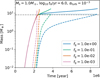 |
Fig. 2 Growth of protoplanets up to crossover mass around 1 M⊙ star with the core formation time t0 = 1 Myrs. Different colors show the cases with different grain opacity fg. The solid, dashed, and dotted lines show the total, envelope, and solid core mass, respectively. The horizontal gray dashed line shows the pebble isolation mass. |
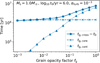 |
Fig. 3 Growth times obtained in the simulations with Ms = 1 M⊙ , t0 = 106 yr, and αturb = 10−3. The solid line shows the crossover time, measured from the core formation time. The dashed and dotted lines show the times required for the protoplanet to grow from M0 to Miso and from Miso to Mcross, respectively. |
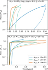 |
Fig. 4 Same as Fig. 2, but for different assumed turbulent viscosities αturb. The upper and lower panels show the cases with fg = 10−2 and fg = 100, respectively. |
3.2 The role of turbulent viscosity
Next, we explore the importance of the assumed disk’s turbulent viscosity. The disk’s turbulent viscosity affects the pebble accretion rate and isolation mass. The pebble accretion rate is higher for lower αturb because of the smaller pebble layer’s scale height (see Eq. (15)). On the other hand, the pebble isolation mass becomes smaller for lower αturb as shown in Eq. (20). Figure 4 shows the time evolution of protoplanets with different αturb. We also plot the crossover time presented in Fig. 5. Here, we show the cases with Ms = 1 M⊕, t0 = 106 yr, and fg = 0.01 (upper panels) and 1 (lower panels). Due to the higher pebble accretion rate, the protoplanet reaches the pebble isolation mass earlier for lower αturb. The planetary core mass is smaller for lower αturb because of the smaller pebble isolation mass. As shown in Fig. 5, the core growth time tg,core is shorter for lower αturb. On the other hand, the contraction time tg,cont is longer for lower αturb. This is because of the smaller pebble isolation mass. The envelope’s contraction timescale strongly depends on the mass of protoplanets (Ikoma et al. 2000; Piso & Youdin 2014).
When the grain opacity is small (for example, fg = 0.01), the core growth time regulates the crossover time as discussed in Sect. 3.1, and the crossover time decreases for lower αturb. On the other hand, when fg = 1, the dominant growth phase is the envelope’s contraction phase, and the crossover time is longer for lower αturb.
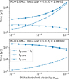 |
Fig. 5 Same as Fig. 3, but for different assumed turbulent viscosities αturb. The upper and lower panels show the cases with fg = 10−2 and fg = 100, respectively. |
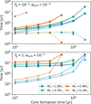 |
Fig. 6 Same as Fig. 3, but for different core formation times t0. The top and bottom panels show the cases with fg = 0.01 and 0.1, respectively. The different colors correspond to different stellar masses. The solid, dashed, and dotted lines show the crossover time measured from the core formation time tg,cross - t0, the core growth time tg,core, and the contraction time tgcont, respectively. Here, we show the cases with αturb = 10−3. |
3.3 Core formation time and stellar mass
Figure 6 shows the crossover time as a function of the core formation time. We show the cases with low grain opacity fg = 0.01 and high grain opacity fg = 1 in the top and bottom panels, respectively. First, we focus on the cases around 1 M⊙ stars (blue lines). We find that the protoplanets take longer to reach the pebble isolation mass (dashed lines) if the core formation time is longer. This is because both the total dust mass remaining in the protoplanetary disk and the pebble flux decrease with time. Unlike in the core growth phase, the growth time in the contraction phase tg,cont (dotted lines) depends only weakly on t0.
We also plot the cases around different stellar masses in Fig. 6. Because of the lower pebble flux, the protoplanet takes longer to reach the pebble isolation mass around lower-mass stars. When fg = 0.01, the protoplanet reaches crossover mass soon after the pebble isolation mass is reached, and tg,cont is rather independent of the mass of the host stars. However, tg,cont depends on the stellar type when fg = 1. The pebble isolation mass is larger for planets around more massive stars. Due to the larger core mass, the planetary envelope contracts quickly, and therefore, tg,cont is shorter around more massive stars.
We find that protoplanets do not reach pebble isolation around very low mass stars Ms = 0.1 Ms. However, the protoplanets could reach the crossover mass if the core formation time is as short as 105 yr and fg = 0.01. In the case of t0 = 105 yr, the protoplanet’s core mass is 1.2 M⊕. Despite the small core mass, the protoplanet can accrete disk gas due to the low atmospheric opacity. With higher grain opacity fg = 1, protoplanets do not reach the crossover mass with Ms = 0.1 Ms.
While the crossover time tg,cross ranges from 105 to 107 yr for lower grain opacity cases fg = 0.01, tg,cross exceeds 5 Myrs for the higher grain opacity cases fg = 1.0. Since observations suggest that typical disk lifetimes are ∼1-3 Myrs (Richert et al. 2018), the frequency of giant planet formation is expected to be low if fg = 1.0. In the next section, we further discuss the occurrence rate of giant planets.
3.4 Crossover time
Figure 7 shows the inferred crossover time tg,cross as a function of stellar mass Ms and core formation time t0 , for different fg and αturb. The crossover time shortens with faster core formation around more massive stars. When fg = 1.0 and αturb = 10−3, giant planet formation is rather slow, and crossover time exceeds 3 Myrs. In that case, only the long-lived protoplane-tary disks would enable the formation of giant planets. When the grain opacity factor is as small as fg = 0.01, the crossover time becomes ∼1 Myr. Giant planets would form if the initial core formation ends within 1 Myrs, except around late M-dwarfs (Ms = 0.1 M⊕).
As shown in Sect. 3.2, a smaller turbulent viscosity of αturb = 10−5 shortens the crossover time if the grain opacity is small as fg = 0.01, but lengthens if fg = 1. A smaller turbulent viscosity αturb = 10−5 and grain opacity fg = 0.01 are required to form giant planets around late M-dwarfs. In this case, the crossover time weakly depends on the stellar type if the initial core forms within 1 Myr. Even if the initial core formation takes t0 ∼ 3 Myrs (log10tg,cross = 6.5), giant planets could still form around high-mass stars with long-lived protoplanetary disks. On the other hand, no giant planets would form with a low turbulent viscosity αturb = 10−5 and a high grain opacity fg = 1.
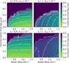 |
Fig. 7 Crossover time obtained from simulations starting with an initial core of Mcore = 0.01 M⊕. We plot the obtained crossover time tg,cross as a color contour, and the color bar is shown on the right side of the panels. The horizontal and vertical axes are stellar mass Ms and the core formation time t0. The black lines show the contour lines and the number on each line shows log10 tg,cross. The left and right columns correspond to the low (fg = 0.01) and high (fg = 1) grain opacity cases. The top and bottom rows show the high (αturb = 10−3) and low (αturb = 10−5) turbulent viscosity cases. |
3.5 From core formation to crossover
In the above sections, we investigate the formation of giant planets, setting the core formation time t0 as an input parameter. Hereafter, we estimate t0 by calculating the pebble accretion onto a protoplanet, which is set to be the largest planetesimal formed by streaming instability. Then, we estimate the crossover timescale using the numerical results obtained in Sect. 3.4.
3.5.1 Core formation time
Hydrodynamic simulations show that the maximum size of planetesimals formed by the streaming instability could be several hundred km in radius (Simon et al. 2017; Schäfer et al. 2017). We estimate the maximum size of planetesimals using two different models. The first model is the model used in Lau et al. (2022), where the characteristic planetesimal size is set by the typical clump size of pebbles determined by the local diffusivity δ, which is given by (Klahr & Schreiber 2020)
 (23)
(23)
 (24)
(24)
The streaming instability simulations by Abod et al. (2019) show that the cumulative mass distribution of planetesimals exhibits an exponential cutoff ~0.3mG. Although such massive planetesimals are relatively rare, planetesimals with masses of ~ mG form via streaming instability. We adopt mG as the maximum planetesimal size mplt. Following Lau et al. (2022), we set δ as a free parameter independent of αturb. We use log10 δ = −4.0, −4.5, and −5.0. The second model is the model by Liu et al. (2020). In this model, the mass of the dust clump is determined by the self-gravity and the tidal shear, which is given by
 (25)
(25)
with
 (26)
(26)
where fplt is the ratio between the maximum mass and the characteristic mass of planetesimals formed by the streaming instability. Liu et al. (2020) estimates fplt as 400 from the streaming instability simulations by Schäfer et al. (2017), but fplt could change with the disk conditions (Simon et al. 2017). To account for this uncertainty, we also use a value of fplt = 40, which is smaller by a factor of ten.
Figure 8 shows the inferred initial mass of the protoplanet. We assume that the first planetesimal forms at t = 105 yr with Mp = mplt. We calculate the planetary growth via pebble accretion without the gas accretion and estimate the core formation time t0 by integrating it up to 10−2M⊕. Then, we estimate the crossover time using the numerical results obtained in Sect. 3. We introduce a fitting function tg,cross,fit(αturb, fg) to the obtained crossover time tg,cross as a function of the core formation time t0 and stellar mass Ms. We use scipy.interpolate.RBFInterpolator to determine the fitting function.
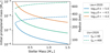 |
Fig. 8 Maximum mass of planetesimals mplt used in our model. The solid lines show the estimated mplt in the model by Lau et al. (2022). The different colors correspond to different δ. The dashed lines show the estimated mplt in the model by Liu et al. (2020). The different color corresponds to different fplt. The right y axis shows the radius of the protoplanet. We use the mean density of 3g/cm3 to estimate the radius. |
3.5.2 Effects of initial protoplanet’s mass
Figure 9 shows the estimated crossover time. We plot the cases using different initial protoplanet masses mplt . First, the protoplanet could not reach the crossover mass when we use Eq. (25) with δ = 10−5. In this case, the mass of the initial protoplanet is ≲10−5 M⊕ and too small to initiate rapid pebble accretion. We present the mass-doubling timescale τpeb in Fig. 10. As shown in this figure, the pebble accretion rate strongly depends on the mass of the growing protoplanet when ≲10−5 M⊕. To initiate rapid pebble accretion, the initial protoplanet’s mass must be larger than ≳10−5 M⊕.
The protoplanet can grow to the crossover mass with the other initial protoplanet mass. For fg = 1, we find that the crossover time rarely depends on the initial protoplanet mass. This is because the growth time in the contraction phase is longer than in the core growth phase.
When the grain opacity factor is small as fg = 0.01, the crossover time is shorter for the larger initial protoplanet mass. However, even if the initial mass was 10 times larger, the crossover time is shortened by 2–3. In the pebble accretion model, the mass-doubling timescale rarely changes with the protoplanet mass when Mp ≳ 10−5 M⊕ as shown in Fig. 10. If the mass doubling timescale τpeb is constant, the protoplanet mass is written as
 (27)
(27)
Since the contraction phase is negligibly shorter than the core growth phase, the time reaching the crossover is given by
 (28)
(28)
Therefore, the crossover time weakly depends on the initial protoplanet mass if the initial planetesimals are born big as ≳10−5 M⊕.
From the above results, we conclude that the protoplanet’s initial size has a minor effect on the crossover time in the pebble accretion scenario, compared to the other parameters, like the grain opacity and stellar mass.
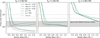 |
Fig. 9 The estimated crossover time in the pebble accretion scenario. The solid and dashed lines show the cases with the planetesimal formation model by Eqs. (24) and (25), respectively. The different colors show the cases with different parameters, as described in the legend box. Each panel shows the cases with different grain opacities. The gray area shows the typical disk lifetime inferred by the observations (Richert et al. 2018), which ranges from 1 to 3 Myrs. We plot the horizontal dotted gray lines at 5 and 10 Myrs for the eye guide. |
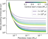 |
Fig. 10 Mass doubling timescale in the pebble accretion model. The solid and dashed lines show the different times t = 105 and 106 yr, respectively. The color corresponds to the different masses of central stars, and the color bar is written on the panel’s upper right. |
3.5.3 Crossover time across different stellar types
We find that the crossover time decreases with increasing stellar mass and changes the dependence on the stellar mass around Ms ~ 0.4 M⊕ as shown in Fig. 9. For planets orbiting around stars of Ms ≲ 0.4 M⊕, the crossover time strongly depends on Ms. These planets could not reach pebble isolation mass before the pebbles in the protoplanetary disk are depleted. The pebble flux is generated by the sweep of the pebble growth line rg. When rg < Rdisk, the pebble flux slowly decreases with time (∝ t−8/21). Once the pebble growth line reaches the disk’s typical radius Rdisk, the pebble flux decreases exponentially because of the reduction in the dust surface density at the disk’s outer edge. By substituting rg = 2 Rdisk into Eq. (18), r = 2 Rdisk gives a ten times reduction in Σgas because of the disk’s outer edge, we obtained the pebble depletion time as
 (29)
(29)
We plot Eq. (29) on the left panel in Fig. 9.
When fg = 0.01, the envelope contraction phase is much shorter than the core growth phase, as we found in Sect. 3. tg,cross < τpeb,dep means that the protoplanet can reach the pebble isolation mass before the pebbles are depleted. The dependence of the crossover time on the stellar mass comes from the core growth time, which decreases with increasing stellar mass because the mass doubling timescale τpeb is shorter around the higher mass stars. On the other hand, the protoplanets could not reach the pebble isolation mass in the cases with tg,cross > τpeb,dep. For these non-isolated protoplanets, the envelope’s contraction takes a longer time because of the smaller core mass. The protoplanet’s core mass is smaller around the smaller mass stars because of the shorter τpeb,dep and longer τpeb. Therefore, the crossover time steeply increases with decreasing stellar mass.
We plot the typical disk lifetime 1-3 Myrs with the gray area in Fig. 9. Using the dust observations in stellar clusters, Richert et al. (2018) found that the disk longevity rarely depends on the stellar mass, and the fraction of stars with disks is 60–70% at 1 Myrs and 30-40% at 3 Myrs. Currently, there is no evidence that the lifetimes of the dust disk and the gas disk are the same. However, it is reasonable to assume that both components could be dispersed by the same mechanisms, such as photoevaporation or disk winds. However, dust growth could lead to the selective removal of small dust grains while leaving the gas behind, and possibly leading to a gaseous disk that survives longer than dust disks inferred from observations. For simplicity, in this study the lifetimes of the dust and gaseous disks are assumed to be equal. Under this assumptions our results suggest that more than 30% of stars heavier than ~0.4 M⊙ have cold Jupiters if fg ≲ 0.1. This result is inconsistent with the observed occurrence rate of cold Jupiters (Fulton et al. 2021), where only ≲20% of G-type stars have cold Jupiters.
To be consistent with the low occurrence rate of cold Jupiters, a higher grain opacity of fg > 0.1 is required. When fg = 1, the crossover time ranges between 5 and 10 Myrs in Ms ≳ 0.4 M⊙. Also, the crossover time decreases with the stellar mass. Due to the high grain opacity, the crossover time is regulated by the envelope’s contraction. The timescale in Kelvin-Helmholtz contraction is given by (Ikoma et al. 2000)
 (30)
(30)
where κenv is the effective opacity in the planetary atmosphere and k2 is estimated 2.5-3.5. In our model, the pebble isolation mass scales as
 (31)
(31)
Using k2 = 3.0 and substituting Mp = Miso, we get τKH ∝ Ms−9/7. The strong dependency between the crossover time and the stellar mass could explain the higher occurrence rate of cold Jupiter around more massive stars, as inferred from observations (Fulton et al. 2021).
The exact occurrence rate also depends on the distribution of the disk’s lifetime. However, the available observational data are limited to t ≤ 5 Myrs in Richert et al. (2018), and the fraction of stars with disks between 5 and 10 Myrs is unclear yet. Recent studies suggest that the characteristic timescale for the disk’s lifetime could be 5-10 Myr (Michel et al. 2021; Pfalzner et al. 2022), which prefers the scenario with the high grain opacity fg = 1 to be consistent with the observed cold Jupiter’s occurrence rate. Since the formation of giant planets is controlled by the gaseous disk’s lifetime, a better understanding of the distribution of disk lifetimes is required.
Also, the gas distribution in the protoplanetary disks was assumed to be smooth. However, this is a clear simplification. Indeed, recent observations of protoplanetary disks show the common existence of substructures such as rings and spirals (e.g. Andrews 2020; Benisty et al. 2023). These substructures would affect the pebble flux and its accretion onto protoplanets. For example, Lau et al. (2022) shows that if planetesimals form and grow in a pressure bump, planetesimal accretion and rapid pebble accretion can occur, leading to the formation of a core of several M⊕ within 105 years. If such substructures shorten the core growth phase, it emphasizes the need for a slow contraction phase. It is therefore clear that a better understanding of the mechanisms by which substructures in protoplanetary disks accelerate or delay the formation of giant planets is required. This will allow us to better connect the properties of the planetary disk and the planetary formation history.
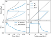 |
Fig. 11 The growth of the planetary core up to the crossover mass accounting for envelope enrichment caused by pebble evaporation. The blue lines show the case with Ms = 1 M⊙, t0 = 106 yr, αturb = 10−3 and fg = 1. The gray lines show the case without envelope enrichment. Panel a: time evolution of total mass (solid line), envelope mass (dashed line), and core mass (dotted line). Panel b: time evolution of the bulk metallicity of planetary envelope. Panel c: evolution of planetary masses as a function of the total mass. Panel b: evolution of the bulk metallic-ity of planetary envelope vs. the total mass of protoplanet. The vertical dashed lines in Panels c and d are pebble isolation mass. |
4 Discussion and caveats
4.1 Heavy-element deposition in the envelope
In the simulations presented above, we neglect the ablation of the accreted pebbles and assume that all the heavy elements settle to the center. However, the enrichment of the envelope with heavy elements accelerates the contraction of the planetary envelope (Hori & Ikoma 2010, 2011; Venturini et al. 2015, 2016; Valletta & Helled 2020; Mol Lous et al. 2024). In this section, we investigate how envelope enrichment changes the crossover time.
We use the ablation model developed by Valletta & Helled (2020) and Mol Lous et al. (2024). We use the direct deposition model, where the ablated heavy elements from the accreted pebbles are deposited into the local envelope shell. We set the pebble composition to be 50% rock and 50% H2O, and assume that only the ablated H2O is deposited in the envelope. We include the condensation of H2O using the saturation pressure and the maximum water enhancement of the supercritical water Zsup,H2O = 0.9. We also introduce the pre-mixing algorithm for heavy elements if the Rayleigh-Taylor criterion is met. Further details of our heavy-element enrichment method are presented in Appendix D. To save computational time, we start with M0 = 0.1 M⊕, instead of M0 = 0.01 M⊕.
Figure 11 shows the planetary evolution including the envelope enrichment by the accreted pebbles. We find that the metallicity in the protoplanet envelope increases quickly and saturates to ~0.8. After reaching the pebble isolation mass, the atmospheric metallicity decreases because only gas accretes to the protoplanet in this phase. We also plot the cases without envelope enrichment with gray lines. Note that these cases differ from the simulations in Sect. 3 because of different M0. Interestingly, we find that the crossover time is longer for the cases with envelope enrichment. The high metallicity of the envelope leads to higher gas accretion rates and larger envelope mass during the core growth phase. Since the total protoplanet mass regulates the pebble isolation mass, the core mass decreases at the pebble isolation compared to the cases without envelope enrichment. Piso & Youdin (2014) shows that the gas accretion rate in the following contraction phase strongly depends on the core mass. Due to the smaller core, the growth time in the contraction phase is longer when envelope enrichment is considered. This situation does not occur in the study of Mol Lous et al. (2024) because the pebble isolation mass was set to ∼25 M⊕ and the protoplanet did not reach the pebble isolation in 10 Myrs.
We also performed simulations with a lower grain opacity factor fg = 0.01 (Fig. 12). Due to the rapid envelope contraction in the contraction phase, the effect of envelope enrichment is weaker. The inferred difference in the crossover time is only <0.3 Myrs.
We find that heavy-element enrichment in the planetary envelopes does not necessarily shorten the formation timescale of giant planets. However, we investigated only a few parameter studies using the specific enrichment parameters (50%-rock-50%-water and Zsup,H2O = 0.9). As shown in Mol Lous et al. (2024), the effect of envelope enrichment is more profound if the accreted pebbles are composed of pure-water because the energy deposited by the accreted pebbles is small. Even with 50%-rock-50%-water, the ablation and deposition of rock, which we assume non-missible to the H-He envelope, would accelerate gas accretion and would change the mass of the planetary core. Future studies should investigate in further detail how the planetary formation timescale changes with envelope enrichment when considering various compositions.
4.2 Extending the envelope contraction phase
We find that a high grain opacity factor of fg > 0.1 is required to explain the low occurrence rate of cold Jupiters. However, dust growth models in planetary envelopes suggest that small dust grains grow to larger sizes and quickly settle to deeper regions, reducing grain opacity (Movshovitz et al. 2010; Mordasini 2014; Ormel 2014). The estimated grain opacity factor is fg ≤ 0.01 (Mordasini 2014). Additional mechanisms that delay the envelope’s contraction, such as gas recycling or a continuous accretion of dust and planetesimals after the protoplanet reached pebble isolation mass, are required.
3D hydrodynamical simulations show that the accreted gas enters the Hill sphere through the poles and exits to the disk’s midplane (Tanigawa et al. 2012; Ormel et al. 2015; Kurokawa & Tanigawa 2018). The recycled gas keeps bringing small dust to the radiative-advective boundary region of the planets, which would lead to a dust opacity comparable to the (local) dust opacity in the disk (Lambrechts & Lega 2017). After pebble isolation mass is reached, the drifting pebbles pile up at the outer pressure bump. This can trigger fragmentation, and dust grains that are small enough to be coupled to the disk gas can flow into the planetary envelope (Stammler et al. 2023). The accretion of small dust could increase the grain opacity in the planetary envelope and may delay the envelope’s contraction (Chen et al. 2020). Further investigation of the grain opacity in protoplan-etary disks, including the grain growth around a protoplanet, should be conducted in future studies.
Another possible mechanism is planetesimal accretion. In this study, we neglected planetesimal accretion after the formation of initial planetesimals. No protoplanets grow via pebble accretion if the initial protoplanet mass mplt is smaller than 10−5 M⊕. However, planetesimal accretion could grow the small planetesimals to a point where they trigger rapid pebble accretion (e.g., Johansen & Lambrechts 2017). The timing of when rapid pebble accretion starts could be later than the time of planetesimal formation, and the crossover time could be more delayed than that obtained in our simulations. Also, we neglected the process of planetesimal accretion, which could take place in parallel to pebble accretion. Unlike pebble accretion, planetesimal accretion could continue even after the gap formation, and accreted planetesimals could provide additional energy to the planetary envelope, delaying the contraction of the planetary envelope (Alibert et al. 2018; Helled 2023). Since planetesimals need to form to start rapid pebble accretion, planetesimal accretion seems to be inevitable during giant planet formation, although the accretion rate could be smaller than that of pebble accretion. In fact, it is possible that pebble accretion and planetesimal accretion dominate at different stages during planet formation as well as in different disk environments. Understanding the interplay between planetesimal accretion and pebble accretion is desirable.
4.3 Effects of disk scaling models
The pebble accretion process strongly depends on the assumed disk model. In our disk model, protoplanets could not reach pebble isolation around stars of ≲0.4 M⊕, and the break point of the crossover time where the dependency on stellar mass changes appears around 0.4 M0. However, as shown in Eq. (29), the pebble depletion time decreases around low-mass stars, and the break point would shift to larger mass if the exponent BC gets larger.
In our model, the disk accretion rate Md,acc scales as
 (32)
(32)
Here, we neglect the viscous evolution and radial decay terms in Σgas. The relation between the disk accretion rate and the stellar mass can be estimated from observations (e.g. Manara et al. 2022), and our scaling law seems to be shallower than that in observations. Single power-law fitting suggests a slope of 1.6-2.. Such a steep slope requires higher A, B, or smaller C than those in our model. However, the exact relation between Ṁd,acc and M⊙ is still actively discussed. Several studies show that a double power-law fit for Ṁd,acc - M0 is a more appropriate representation than a simple power-law fit (Alcalá et al. 2017; Manara et al. 2017). In this case, the slope is flatter for stars more massive than 0.2-0.3 M0. Note that the observed disk accretion rate is time-dependent and that the exact scaling law at time zero remains unknown. A more robust determination of the properties of disks around different stellar types is important for constraining the origin of cold Jupiters and predicting their occurrence rate.
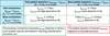 |
Fig. 13 A summary of our results and the inferred giant planet formation regimes. |
4.4 Planetary migration
For simplicity, planetary migration is not included in this study. However, it is clear that planet migration plays an important role in planet formation. The migration regime typically changes from type I to type II around the pebble isolation mass (∼10 M⊕), and the migration speed peaks around this transition (Kanagawa et al. 2018; Ida et al. 2018). When the grain opacity is as high as fg = 1, the protoplanet enters a long contraction phase after reaching pebble isolation mass. During this phase, the protoplanet can undergo significant radial migration, potentially becoming a warm or hot Jupiter. In contrast, when the grain opacity is low, for example, fg = 0.01, the protoplanet grows rapidly after pebble isolation mass is reached (see Fig. 3) and quickly shifts to the slower type II migration. Figure 13 is the summary of our findings. This quick transition to slower migration could help prevent significant inward migration. Note, however, that it remains unclear whether such low grain opacities are common.
While inward migration is expected to occur, outward migration (Paardekooper et al. 2010, 2011; Paardekooper 2014), and migration trap (Masset et al. 2006; Coleman & Nelson 2016) could also take place. Outward migration occurs near the transition radius, where the dominant disk heating mechanism shifts from viscous accretion to stellar irradiation (Liu et al. 2019, 2020). However, this mechanism weakens as the planet grows in mass and the disk evolves. Alternative mechanisms are disk substructures that can act as migration traps, enabling the survival of cold Jupiters (Coleman & Nelson 2016). Both outward migration and migration traps are sensitive to the evolving disk structure. A more comprehensive understanding of the formation of “cold” giant planets will require future investigations that incorporate planetary migration self-consistently, ideally through disk evolution models and hydrodynamical simulations.
If significant planetary migration occurs, a quick transition to slower type II migration might be required. To be consistent with the lower occurrence rate of cold Jupiters, planetary cores should form less efficiently. Our model assumes that icy pebbles are sticky and continue to grow until the gas drag from the disk causes the growing pebbles to drift inward. However, recent observations of dust in protoplanetary disks (Jiang et al. 2024) and laboratory experiments (Musiolik et al. 2016) suggest that icy pebbles are more fragile and pebbles initiate fragmentation even outside the water ice line. If this is the case, the pebble accretion efficiency is reduced due to the lower Stokes number. Since the planetary core growth takes longer, giant planets would form less efficiently, even if the grain opacity is lower than fg = 1. Fragile icy pebbles may support the formation of cold Jupiters.
It remains unclear how planet migration takes place in disks around different stellar types and we are still lacking a good understanding of how the disk properties (for example, density, lifetime) change with the mass of the central star. As a result, it is still unclear whether different migration histories are expected. Future studies should investigate how planetary migration affects planet formation across different stellar masses.
5 Summary and conclusions
We investigated the formation of cold Jupiters around different mass stars. We explored how the crossover time changes with stellar mass Ms, core formation time t0, grain opacity factor fg, and disk turbulent viscosity αturb, assuming pebble accretion. Our key conclusions can be summarized as follows:
The grain opacity strongly affects the planetary growth. If the grain opacity is lower than fg ≲ 0.1, the crossover time is comparable to the growth timescale of the heavy-element core. Contrary, if fg ≳ 0.1, the envelope contraction dominates the formation process, and the protoplanets experience a long envelope contraction phase after reaching the pebble isolation mass.
Low disk turbulent viscosity αturb accelerates (delays) reaching crossover mass when the grain opacity is lower (higher) than fg ~ 0.1. When fg < 0.1, the core growth time decreases for lower αturb because of the smaller pebble layer’s scale height and higher pebble accretion rate. On the other hand, the envelope contraction timescale increases because of the lower pebble isolation mass if fg > 0.1.
The crossover time depends on the initial size of protoplanets. However, this dependency is weaker than linear. The grain opacity plays a bigger role than the initial size of protoplanets in determining the crossover time.
Around stars of Ms ≲ 0.4 M0, the crossover time rapidly increases with decreasing stellar mass. Around these stars, pebbles in the protoplanetary disk deplete before the protoplanets reach pebble isolation mass. Because of the small mass of the forming solid core, the envelope’s contraction timescale (before reaching the crossover mass) is long. A very long disk lifetime ≳107 yr, as found in Peter Pan disks, is required to form giant planets around such stars.
Around stars with masses Ms ≳ 0.4 M0, protoplanets reach crossover mass within 3 Myrs if the grain opacity is fg ≲ 0.1, which is comparable or shorter than the typical disk’s lifetime. To be consistent with the low occurrence rate of cold Jupiters around G-type stars (≲20%), a high grain opacity (fg > 0.1) is required. With a high grain opacity fg = 1, the crossover timescale increases around lower-mass stars, which could explain the inferred low-occurrence rate of cold Jupiters around small stars.
We find that the crossover time can be divided into two regimes by comparing the core formation time tg,core and the pebble depletion timescale τpeb,dep. In the fast pebble depletion regime where τpeb,dep < tg,core, the protoplanet does not reach the pebble isolation mass, and the crossover time exceeds 10 Myrs because of the small core mass. Giant planets may form in a long-lived disk, such as the Peter-Pan disk, but this formation path would not be the primary formation path of cold Jupiters around FGK-type of stars.
If the planetary core forms before the pebbles are depleted (slow pebble depletion regime where τpeb,dep > tg,core), the protoplanet can grow to the pebble isolation mass. To account for the observed low occurrence rate of cold Jupiters around G-type stars, either slow envelope contraction or slow core formation – lasting longer than the typical disk lifetim – is required. In our pebble accretion model, protoplanets quickly reach the pebble isolation mass and therefore, a slow contraction of the planetary envelope is required to suppress giant planet formation and explain the low occurrence rate of cold Jupiters. This result is consistent with recent formation models that suggest that the formation of Jupiter and Saturn could have taken a few million years (Alibert et al. 2018; Helled 2023). However, rapid contraction may be required to form giant planets around lower-mass stars. This result may indicate that the metallicity and dust content of protoplanetary disks increase with the mass of the central stars. Indeed, it was recently shown that the bulk metallicity of giant planets is lower for giant planets orbiting small stars in comparison to giant planets around sun-like stars (Müller & Helled 2025). The relationship between the heavy-element mass in the disk and stellar mass is yet to be determined, and is likely to control giant planet formation around different stellar masses.
Interestingly, we found that envelope enrichment with heavy elements released from accreted pebbles could delay envelope contraction, a different result from that obtained in previous studies. Because of the higher mean molecular weight, the protoplanets could have a more massive envelope at the pebble isolation mass. Consequently, the core mass at the pebble isolation is smaller when envelope enrichment is considered. Due to the smaller core mass, the envelope contracts more slowly, resulting in a delayed crossover time. Our results also do not rule out the possibility of slow core formation. The timescale for core growth depends sensitively on disk structure, metallicity, and the dust fragmentation velocity.
We note that the durations of core formation and envelope contraction depend on the formation history and, therefore, on various processes and parameters. The core formation timescale strongly depends on the local conditions in the disk and the types of solids that are accreted. Similarly, while in this study, a slow contraction phase is achieved with a high grain opacity, delaying the envelope contraction could be the result of other mechanisms, such as atmospheric recycling or planetesimal accretion. It is therefore clear that a better understanding of the conditions and processes taking place during planet formation is crucial. Overall, our findings highlight the complex interplay between core accretion, envelope physics, and disk evolution in shaping planetary outcomes. We suggest that future studies should include these processes self-consistently and investigate a wide parameter space. Only then can we reveal the origin of cold Jupiters in our galaxy.
Acknowledgements
The numerical computations were carried out on PC cluster at the Center for Computational Astrophysics, National Astronomical Observatory of Japan. R.H. acknowledges support from SNSF under grant 200020_215634.
Appendix A Solid mass conservation
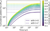 |
Fig. A.1 Time evolution of the cumulative pebble flux. The solid lines show the cumulative pebble flux calculated with Eq. 17. The dashed lines are those obtained with Eq. 17 using the time evolving Σgas(t = t′) instead of Σgas(t = 0). The horizontal dotted lines show the initial total mass of solids in the protoplanetary disk. The different colors correspond to disks around different stellar masses. |
In Eq. 17 we use the solid surface density at t = 0 instead of that at t = t′, where t′ is the disk’s age. Using Σgas(t = t′) in Eq. 17 would account for the radial transport of small dust grains due to gas advection and diffusion, and thus seems more realistic than using Σgas(t = 0). However, this approach overestimates the pebble flux. This is because the gas that diffuses outward from r < Rdisk to r > Rdisk may be depleted of solids. For simplicity, we do not consider this effect in our model.
To illustrate this point, we plot the cumulative pebble flux calculated with Eq. 17 using Σgas(t = 0) (solid lines) and Σgas(t = t′) (dashed lines). We find that the two models yield similar evolution up to t′ ~ τvis, but the model using Σgas(t = t′) eventually overestimates the pebble flux and violates mass conservation by exceeding the initial total solid mass. To preserve mass conservation, we adopt Σgas(t = 0) in Eq. 17.
Our pebble flux model is valid only if the pebble condensation front reaches the outer edge of the disk before the gaseous disk starts viscous evolution, when τpeb,dep ≲ τvis. For disks with higher viscosity or larger radial extent, a more sophisticated model of dust evolution is required to compute the pebble flux accurately.
Appendix B Mixing length parameter
To check the effect of different mixing length parameter αMLT, we compare the simulations with αMLT = 2 (solid lines) and αMLT = 0.1 (dashed lines) in Fig. B.1. We found that the difference in the obtained crossover time is less than 5%. We conclude that the effect of αMLT is negligibly smaller than that of the other parameters, such as stellar mass Ms and the grain opacity factor fg.
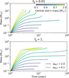 |
Fig. B.1 The evolution of protoplanets around different mass stars using different αMLT = 2 (solid lines) and αMLT = 0.1 (dashed lines). The top and bottom panels show the cases with different grain opacity factors fg = 0.01 and 1, respectively. The color corresponds to the stellar mass, as shown in the color bar. |
Appendix C Supply-limited gas accretion
In our simulations, the gas accretion rate is obtained by iterating the planetary radius and the gas accretion radius. The energy balance in the planetary envelope determines the gas accretion rate in this phase. However, the gas accretion rate onto the protoplanet could be limited by the supply of local disk gas to the planetary orbital region. Once the envelope’s contraction and the following gas accretion become fast enough to deplete local disk gas, the planetary envelope detaches from the protoplane-tary disk, and the accretion regime shifts to supply-limited gas accretion. Here, we compare our numerical results to the maximum supply of disk gas and discuss how supply-limited gas accretion affects our results.
To estimate the maximum supply of disk gas, we follow the approach developed by Tanaka et al. (2020). The flux of disk gas entering the protoplanet’s Hill sphere is given by (Tanigawa & Watanabe 2002)
 (C.1)
(C.1)
with:
 (C.2)
(C.2)
Σband is the gas surface density at the gas accretion band. Protoplanets massive enough to open a gap in the gaseous disk reduce the local gas surface density and Σband. Using the gap structure model obtained by Kanagawa et al. (2017), we get
 (C.3)
(C.3)
with
 (C.4)
(C.4)
Equation C.1 shows the limit of gas disk supply through the local gas flow. In addition, the global disk accretion Md,acc limits the supply of disk gas onto protoplanets. Finally, the maximum supply of disk gas is
 (C.5)
(C.5)
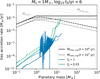 |
Fig. C.1 Gas accretion rate obtained in our numerical simulations of Ms = 1M⊙ and log10t0/yr = 6. The blue and green lines show the cases with fg = 1 and 0.01, respectively. The solid and dashed lines correspond to the cases with αturb = 10−3 and 10−5, respectively. We also plot the maximum gas accretion rate in the supply-limited case with black (t = 106 yr) and gray (t = 107 yr) lines. Also, the solid and dashed lines correspond to cases with αturb = 10−3 and αturb = 10−5, respectively. The thin gray dotted lines |
Fig. C.1 shows the gas accretion rate obtained in our simulations and the maximum supply of disk gas Mmax,sup. In most of the simulation phase, the gas accretion rate is slower than Mmax,sup. In simulations with fg = 0.01, the gas accretion rate reaches Mmax,sup just before the crossover mass is reached. Around the crossover mass, the gas accretion timescale is much shorter than the disk’s lifetime. Therefore, even when we include the effects of supply-limited gas accretion, the crossover time obtained in our simulations remains similar.
Appendix D Heavy-element deposition in the gaseous atmosphere
We use the ablation model presented by Valletta & Helled (2020) and Mol Lous et al. (2024). We use the direct deposition model, where the ablated heavy elements (from the pebbles) are deposited into the local envelope shell. We set the composition of pebbles as 50 % rock and 50 % H2O, and assume that only the ablated H2O is deposited in the envelope.
Valletta & Helled (2020) and Mol Lous et al. (2024) introduced the condensation of H2O by putting the maximum metal-licity of a local layer Zmax,i (index-i increases toward the center of the protoplanet). The first limit is the saturation of H2O Zsat,H2O. Using the saturation pressure Psat,H2O, Zsat,H2O is defined as Psat,H2O/Pi where Pi is the local total pressure. The second limit is the maximum water enhancement of the supercritical water ZH2O, which is set to 0.9, as used in Mol Lous et al. (2024).
In addition, Mol Lous et al. (2024) introduced a smoothing factor fsmooth to limit the jump in the local metallicity Zi. Pebbles are usually evaporated in the upper atmosphere and sink to the lower envelope. A large fraction of the heavy elements are deposited in the layer where Zsat,H2O becomes ≳ 0.1. This sink of heavy elements leads to a rather large jump in Zi. As a result, it is not easy for MESA to find a hydrostatic solution. To avoid a large jump in Zi, Mol Lous et al. (2024) introduced a smoothing factor Zsmooth,i = Zpre,i + fsmooth, where Zpre,i is the local metallicity in the previous step.
The maximum metallicity of the local layer i is given by
 (D.1)
(D.1)
If the deposition of the accreted heavy elements leads to a local metallicity Zi that is higher than Zmax,i, the overabundant heavy elements settle to the lower layer. The smoothing factor coefficient fsmooth is set to 0.2. The smoothing factor makes the composition gradient slightly shallower than that without it. This difference in the composition gradient has a weak effect on the crossover time. We found that with the smoothing factor, the crossover times could be 5% shorter at most than those obtained without it. This is because the solid core mass at the pebble isolation becomes slightly larger due to the shallower compositional gradient and the smaller envelope metallicity. This difference does not alter our main finding that the crossover time could be longer if the heavy element deposition is included in the planetary envelope.
Pebbles evaporated in the upper atmosphere create an increasing composition gradient toward the outer envelope. MESA tries to erase this inverted composition gradient by triggering the convection under the Ledoux criterion. However, it makes the timestep too small to proceed, and numerical convergence can be difficult. To avoid this, we introduce a pre-mixing algorithm that assumes Rayleigh-Taylor instability. We cannot use the actual criterion for Rayleigh-Taylor, which compares the density of adjacent layers, because our enrichment model increases the metallicity of local shells without changing the mass there (see Valletta & Helled 2020). Instead, we use this simplified criterion that checks the metallicity of adjacent layers. We mix heavy elements in and distribute them equally to the adjacent two shells if Zi > Zi + 1.
References
- Abod, C. P., Simon, J. B., Li, R., et al. 2019, Astrophys. J., 883, 192 [Google Scholar]
- Alcalá, J. M., Manara, C. F., Natta, A., et al. 2017, A&A, 600, A20 [NASA ADS] [CrossRef] [EDP Sciences] [Google Scholar]
- Alibert, Y., Mordasini, C., & Benz, W. 2011, A&A, 526, A63 [NASA ADS] [CrossRef] [EDP Sciences] [Google Scholar]
- Alibert, Y., Venturini, J., Helled, R., et al. 2018, Nat. Astron., 2, 873 [NASA ADS] [CrossRef] [Google Scholar]
- Andrews, S. M. 2020, Annu. Rev. A&A, 58, 483 [Google Scholar]
- Andrews, S. M., Wilner, D. J., Hughes, A. M., Qi, C., & Dullemond, C. P. 2010, ApJ, 723, 1241 [Google Scholar]
- Andrews, S. M., Rosenfeld, K. A., Kraus, A. L., & Wilner, D. J. 2013, Astrophys. J., 771, 129 [Google Scholar]
- Bai, X.-N., Ye, J., Goodman, J., & Yuan, F. 2016, Astrophys. J., 818, 152 [Google Scholar]
- Bayo, A., Barrado, D., Huélamo, N., et al. 2012, A&A, 547, A80 [NASA ADS] [CrossRef] [EDP Sciences] [Google Scholar]
- Benisty, M., Dominik, C., Follette, K., et al. 2023, in Astronomical Society of the Pacific Conference Series, 534, Protostars and Planets VII, ed. S. Inutsuka, Y. Aikawa, T. Muto, K. Tomida, & M. Tamura, 605 [Google Scholar]
- Bitsch, B., & Savvidou, S. 2021, A&A, 647, A96 [NASA ADS] [CrossRef] [EDP Sciences] [Google Scholar]
- Bitsch, B., Lambrechts, M., & Johansen, A. 2015, A&A, 582, A112 [NASA ADS] [CrossRef] [EDP Sciences] [Google Scholar]
- Bitsch, B., Morbidelli, A., Johansen, A., et al. 2018, A&A, 612, A30 [NASA ADS] [CrossRef] [EDP Sciences] [Google Scholar]
- Bonomo, A. S., Dumusque, X., Massa, A., et al. 2023, A&A, 677, A33 [NASA ADS] [CrossRef] [EDP Sciences] [Google Scholar]
- Boss, A. P. 2006, Astrophys. J., 643, 501 [Google Scholar]
- Boss, A. P. 2019, Astrophys. J., 884, 56 [Google Scholar]
- Burn, R., Schlecker, M., Mordasini, C., et al. 2021, A&A, 656, A72 [NASA ADS] [CrossRef] [EDP Sciences] [Google Scholar]
- Chachan, Y., & Lee, E. J. 2023, Astrophys. J. Lett., 952, L20 [Google Scholar]
- Chen, Y.-X., Li, Y.-P., Li, H., & Lin, D. N. C. 2020, Astrophys. J., 896, 135 [Google Scholar]
- Chiang, E. I., & Goldreich, P. 1997, Astrophys. J., 490, 368 [Google Scholar]
- Choi, J., Dotter, A., Conroy, C., et al. 2016, Astrophys. J., 823, 102 [Google Scholar]
- Coleman, G. A. L., & Nelson, R. P. 2016, Mon. Not. R. Astron. Soc., 460, 2779 [Google Scholar]
- Feng, F., Shectman, S. A., Clement, M. S., et al. 2020, Astrophys. J. Suppl. Ser., 250, 29 [Google Scholar]
- Fulton, B. J., Rosenthal, L. J., Hirsch, L. A., et al. 2021, ApJS, 255, 14 [NASA ADS] [CrossRef] [Google Scholar]
- Guo, K., Ogihara, M., Ida, S., et al. 2025, Astrophys. J., 983, 56 [Google Scholar]
- Helled, R. 2023, A&A, 675, L8 [NASA ADS] [CrossRef] [EDP Sciences] [Google Scholar]
- Hirsch, L. A., Rosenthal, L., Fulton, B. J., et al. 2021, Astron. J., 161, 134 [Google Scholar]
- Hori, Y., & Ikoma, M. 2010, ApJ, 714, 1343 [NASA ADS] [CrossRef] [Google Scholar]
- Hori, Y., & Ikoma, M. 2011, Mon. Not. R. Astron. Soc., 416, 1419 [Google Scholar]
- Ida, S., & Lin, D. N. C. 2005, Astrophys. J., 626, 1045 [Google Scholar]
- Ida, S., Guillot, T., & Morbidelli, A. 2016, A&A, 591, A72 [NASA ADS] [CrossRef] [EDP Sciences] [Google Scholar]
- Ida, S., Tanaka, H., Johansen, A., Kanagawa, K. D., & Tanigawa, T. 2018, Astrophys. J., 864, 77 [Google Scholar]
- Ikoma, M., Nakazawa, K., & Emori, H. 2000, Astrophys. J., 537, 1013 [Google Scholar]
- Inaba, S., Wetherill, G. W., & Ikoma, M. 2003, Icarus, 166, 46 [Google Scholar]
- Jiang, H., Macías, E., Guerra-Alvarado, O. M., & Carrasco-González, C. 2024, A&A, 682, A32 [NASA ADS] [CrossRef] [EDP Sciences] [Google Scholar]
- Johansen, A., & Lambrechts, M. 2017, Annu. Rev. Earth Planet. Sci., 45, 359 [Google Scholar]
- Johnson, J., Howard, A., Marcy, G., et al. 2009, PASP, 122, 149 [Google Scholar]
- Kanagawa, K. D., Tanaka, H., Muto, T., & Tanigawa, T. 2017, PASJ, 69, 6 [Google Scholar]
- Kanagawa, K. D., Tanaka, H., & Szuszkiewicz, E. 2018, Astrophys. J., 861, 140 [Google Scholar]
- Klahr, H., & Schreiber, A. 2020, ApJ, 901, 54 [NASA ADS] [CrossRef] [Google Scholar]
- Kobayashi, H., & Tanaka, H. 2021, ApJ, 922, 16 [NASA ADS] [CrossRef] [Google Scholar]
- Kobayashi, H., & Tanaka, H. 2023, ApJ, 954, 158 [NASA ADS] [CrossRef] [Google Scholar]
- Kurokawa, H., & Tanigawa, T. 2018, Mon. Not. R. Astron. Soc., 479, 635 [Google Scholar]
- Lambrechts, M., & Johansen, A. 2012, A&A, 544, A32 [NASA ADS] [CrossRef] [EDP Sciences] [Google Scholar]
- Lambrechts, M., & Johansen, A. 2014, A&A, 572, A107 [NASA ADS] [CrossRef] [EDP Sciences] [Google Scholar]
- Lambrechts, M., & Lega, E. 2017, A&A, 606, A146 [NASA ADS] [CrossRef] [EDP Sciences] [Google Scholar]
- Lambrechts, M., Johansen, A., & Morbidelli, A. 2014, A&A, 572, A35 [NASA ADS] [CrossRef] [EDP Sciences] [Google Scholar]
- Lau, T. C. H., Dra˛z˙kowska, J., Stammler, S. M., Birnstiel, T., & Dullemond, C. P. 2022, A&A, 668, A170 [NASA ADS] [CrossRef] [EDP Sciences] [Google Scholar]
- Leconte, J., & Chabrier, G. 2012, A&A, 540, A20 [NASA ADS] [CrossRef] [EDP Sciences] [Google Scholar]
- Liu, B., Lambrechts, M., Johansen, A., & Liu, F. 2019, A&A, 632, A7 [NASA ADS] [CrossRef] [EDP Sciences] [Google Scholar]
- Liu, B., Lambrechts, M., Johansen, A., Pascucci, I., & Henning, T. 2020, A&A, 638, A88 [EDP Sciences] [Google Scholar]
- Lynden-Bell, D., & Pringle, J. E. 1974, MNRAS, 168, 603 [Google Scholar]
- Manara, C. F., Testi, L., Herczeg, G. J., et al. 2017, A&A, 604, A127 [NASA ADS] [CrossRef] [EDP Sciences] [Google Scholar]
- Manara, C. F., Ansdell, M., Rosotti, G. P., et al. 2022, Protostars and Planets VII (Tucson: University of Arizona Press) [Google Scholar]
- Masset, F. S., Morbidelli, A., Crida, A., & Ferreira, J. 2006, Astrophys. J., 642, 478 [Google Scholar]
- Mercer, A., & Stamatellos, D. 2020, A&A, 633, A116 [NASA ADS] [CrossRef] [EDP Sciences] [Google Scholar]
- Michel, A., van der Marel, N., & Matthews, B. C. 2021, Astrophys. J., 921, 72 [Google Scholar]
- Miguel, Y., Cridland, A., Ormel, C. W., Fortney, J. J., & Ida, S. 2019, Mon. Not. R. Astron. Soc., 491, 1998 [Google Scholar]
- Mizuno, H. 1980, Prog. Theor. Phys., 64, 544 [Google Scholar]
- Mol Lous, M., Mordasini, C., & Helled, R. 2024, A&A, 685, A22 [NASA ADS] [CrossRef] [EDP Sciences] [Google Scholar]
- Montet, B. T., Crepp, J. R., Johnson, J. A., Howard, A. W., & Marcy, G. W. 2014, Astrophys. J., 781, 28 [Google Scholar]
- Morales, J. C., Mustill, A., Ribas, I., et al. 2019, Science, 365, 1441 [NASA ADS] [CrossRef] [Google Scholar]
- Mordasini, C. 2014, A&A, 572, A118 [NASA ADS] [CrossRef] [EDP Sciences] [Google Scholar]
- Movshovitz, N., Bodenheimer, P. H., Podolak, M., & Lissauer, J. J. 2010, Icarus, 209, 616 [NASA ADS] [CrossRef] [Google Scholar]
- Musiolik, G., Teiser, J., Jankowski, T., & Wurm, G. 2016, ApJ, 827, 63 [NASA ADS] [CrossRef] [Google Scholar]
- Müller, S., & Helled, R. 2025, A&A, 693, L4 [NASA ADS] [CrossRef] [EDP Sciences] [Google Scholar]
- Müller, S., Helled, R., & Cumming, A. 2020, A&A, 638, A121 [Google Scholar]
- Ormel, C. W. 2014, ApJ, 789, L18 [Google Scholar]
- Ormel, C. W., & Klahr, H. H. 2010, A&A, 520, A43 [NASA ADS] [CrossRef] [EDP Sciences] [Google Scholar]
- Ormel, C. W., Shi, J.-M., & Kuiper, R. 2015, Mon. Not. R. Astron. Soc., 447, 3512 [Google Scholar]
- Paardekooper, S.-J. 2014, Mon. Not. R. Astron. Soc., 444, 2031 [Google Scholar]
- Paardekooper, S.-J., Baruteau, C., Crida, A., & Kley, W. 2010, Mon. Not. R. Astron. Soc., 401, 1950 [Google Scholar]
- Paardekooper, S.-J., Baruteau, C., & Kley, W. 2011, Mon. Not. R. Astron. Soc., 410, 293 [Google Scholar]
- Pan, M., Liu, B., Johansen, A., et al. 2024, A&A, 682, A89 [NASA ADS] [CrossRef] [EDP Sciences] [Google Scholar]
- Pan, M., Liu, B., Jiang, L., et al. 2025, Astrophys. J., 985, 7 [Google Scholar]
- Pass, E. K., Winters, J. G., Charbonneau, D., et al. 2023, Astron. J., 166, 11 [Google Scholar]
- Paxton, B., Bildsten, L., Dotter, A., et al. 2011, Astrophys. J. Suppl. Ser., 192, 3 [Google Scholar]
- Paxton, B., Schwab, J., Bauer, E. B., et al. 2018, ApJS, 234, 34 [NASA ADS] [CrossRef] [Google Scholar]
- Pfalzner, S., Dehghani, S., & Michel, A. 2022, Astrophys. J. Lett., 939, L10 [Google Scholar]
- Picogna, G., Ercolano, B., & Espaillat, C. C. 2021, MNRAS, 508, 3611 [NASA ADS] [CrossRef] [Google Scholar]
- Piso, A.-M. A., & Youdin, A. N. 2014, ApJ, 786, 21 [NASA ADS] [CrossRef] [Google Scholar]
- Pollack, J. B., Hubickyj, O., Bodenheimer, P., et al. 1996, Icarus, 124, 62 [NASA ADS] [CrossRef] [Google Scholar]
- Quirrenbach, A., Passegger, V. M., Trifonov, T., et al. 2022, A&A, 663, A48 [NASA ADS] [CrossRef] [EDP Sciences] [Google Scholar]
- Ramirez, R. M., & Kaltenegger, L. 2014, Astrophys. J. Lett., 797, L25 [Google Scholar]
- Ribas, Á., Bouy, H., & Merín, B. 2015, A&A, 576, A52 [NASA ADS] [CrossRef] [EDP Sciences] [Google Scholar]
- Ribas, I., Reiners, A., Zechmeister, M., et al. 2023, A&A, 670, A139 [NASA ADS] [CrossRef] [EDP Sciences] [Google Scholar]
- Richert, A. J. W., Getman, K. V., Feigelson, E. D., et al. 2018, Mon. Not. R. Astron. Soc., 477, 5191 [Google Scholar]
- Rosenthal, L. J., Fulton, B. J., Hirsch, L. A., et al. 2021, Astrophys. J. Suppl. Ser., 255, 8 [Google Scholar]
- Schlecker, M., Burn, R., Sabotta, S., et al. 2022, A&A, 664, A180 [NASA ADS] [CrossRef] [EDP Sciences] [Google Scholar]
- Schäfer, U., Yang, C.-C., & Johansen, A. 2017, A&A, 597, A69 [Google Scholar]
- Shakura, N. I., & Sunyaev, R. A. 1973, A&A, 24, 337 [NASA ADS] [Google Scholar]
- Silverberg, S. M., Wisniewski, J. P., Kuchner, M. J., et al. 2020, ApJ, 890, 106 [NASA ADS] [CrossRef] [Google Scholar]
- Simon, J. B., Armitage, P. J., Youdin, A. N., & Li, R. 2017, Astrophys. J. Lett., 847, L12 [Google Scholar]
- Stammler, S. M., Lichtenberg, T., Dra˛z˙kowska, J., & Birnstiel, T. 2023, A&A, 670, L5 [NASA ADS] [CrossRef] [EDP Sciences] [Google Scholar]
- Tanaka, H., Takeuchi, T., & Ward, W. R. 2002, Astrophys. J., 565, 1257 [Google Scholar]
- Tanaka, H., Murase, K., & Tanigawa, T. 2020, ApJ, 891, 143 [NASA ADS] [CrossRef] [Google Scholar]
- Tanigawa, T., & Watanabe, S.-I. 2002, ApJ, 580, 506 [NASA ADS] [CrossRef] [Google Scholar]
- Tanigawa, T., Ohtsuki, K., & Machida, M. N. 2012, Astrophys. J., 747, 47 [Google Scholar]
- Valencia, D., Guillot, T., Parmentier, V., & Freedman, R. S. 2013, ApJ, 775, 10 [NASA ADS] [CrossRef] [Google Scholar]
- Valletta, C., & Helled, R. 2020, Astrophys. J., 900, 133 [Google Scholar]
- Venturini, J., Alibert, Y., Benz, W., & Ikoma, M. 2015, A&A, 576, A114 [NASA ADS] [CrossRef] [EDP Sciences] [Google Scholar]
- Venturini, J., Alibert, Y., & Benz, W. 2016, A&A, 596, A90 [NASA ADS] [CrossRef] [EDP Sciences] [Google Scholar]
- Venturini, J., Ronco, M. P., Guilera, O. M., et al. 2024, A&A, 686, L9 [NASA ADS] [CrossRef] [EDP Sciences] [Google Scholar]
All Tables
All Figures
|
Fig. 1 Disk model used in this work. Panels a–c show the surface density of the gaseous disk, disk temperature, and the disk’s aspect ratio around different stellar masses as shown in the color bar in panel a. The horizontal dashed line in panel b shows Tdisk = 170 K, where H2O condenses. Here, we show the case when t = 105 yr. |
| In the text | |
|
Fig. 2 Growth of protoplanets up to crossover mass around 1 M⊙ star with the core formation time t0 = 1 Myrs. Different colors show the cases with different grain opacity fg. The solid, dashed, and dotted lines show the total, envelope, and solid core mass, respectively. The horizontal gray dashed line shows the pebble isolation mass. |
| In the text | |
|
Fig. 3 Growth times obtained in the simulations with Ms = 1 M⊙ , t0 = 106 yr, and αturb = 10−3. The solid line shows the crossover time, measured from the core formation time. The dashed and dotted lines show the times required for the protoplanet to grow from M0 to Miso and from Miso to Mcross, respectively. |
| In the text | |
|
Fig. 4 Same as Fig. 2, but for different assumed turbulent viscosities αturb. The upper and lower panels show the cases with fg = 10−2 and fg = 100, respectively. |
| In the text | |
|
Fig. 5 Same as Fig. 3, but for different assumed turbulent viscosities αturb. The upper and lower panels show the cases with fg = 10−2 and fg = 100, respectively. |
| In the text | |
|
Fig. 6 Same as Fig. 3, but for different core formation times t0. The top and bottom panels show the cases with fg = 0.01 and 0.1, respectively. The different colors correspond to different stellar masses. The solid, dashed, and dotted lines show the crossover time measured from the core formation time tg,cross - t0, the core growth time tg,core, and the contraction time tgcont, respectively. Here, we show the cases with αturb = 10−3. |
| In the text | |
|
Fig. 7 Crossover time obtained from simulations starting with an initial core of Mcore = 0.01 M⊕. We plot the obtained crossover time tg,cross as a color contour, and the color bar is shown on the right side of the panels. The horizontal and vertical axes are stellar mass Ms and the core formation time t0. The black lines show the contour lines and the number on each line shows log10 tg,cross. The left and right columns correspond to the low (fg = 0.01) and high (fg = 1) grain opacity cases. The top and bottom rows show the high (αturb = 10−3) and low (αturb = 10−5) turbulent viscosity cases. |
| In the text | |
|
Fig. 8 Maximum mass of planetesimals mplt used in our model. The solid lines show the estimated mplt in the model by Lau et al. (2022). The different colors correspond to different δ. The dashed lines show the estimated mplt in the model by Liu et al. (2020). The different color corresponds to different fplt. The right y axis shows the radius of the protoplanet. We use the mean density of 3g/cm3 to estimate the radius. |
| In the text | |
|
Fig. 9 The estimated crossover time in the pebble accretion scenario. The solid and dashed lines show the cases with the planetesimal formation model by Eqs. (24) and (25), respectively. The different colors show the cases with different parameters, as described in the legend box. Each panel shows the cases with different grain opacities. The gray area shows the typical disk lifetime inferred by the observations (Richert et al. 2018), which ranges from 1 to 3 Myrs. We plot the horizontal dotted gray lines at 5 and 10 Myrs for the eye guide. |
| In the text | |
|
Fig. 10 Mass doubling timescale in the pebble accretion model. The solid and dashed lines show the different times t = 105 and 106 yr, respectively. The color corresponds to the different masses of central stars, and the color bar is written on the panel’s upper right. |
| In the text | |
|
Fig. 11 The growth of the planetary core up to the crossover mass accounting for envelope enrichment caused by pebble evaporation. The blue lines show the case with Ms = 1 M⊙, t0 = 106 yr, αturb = 10−3 and fg = 1. The gray lines show the case without envelope enrichment. Panel a: time evolution of total mass (solid line), envelope mass (dashed line), and core mass (dotted line). Panel b: time evolution of the bulk metallicity of planetary envelope. Panel c: evolution of planetary masses as a function of the total mass. Panel b: evolution of the bulk metallic-ity of planetary envelope vs. the total mass of protoplanet. The vertical dashed lines in Panels c and d are pebble isolation mass. |
| In the text | |
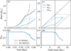 |
Fig. 12 Same as Fig. 11, but with fg = 0.01. |
| In the text | |
|
Fig. 13 A summary of our results and the inferred giant planet formation regimes. |
| In the text | |
|
Fig. A.1 Time evolution of the cumulative pebble flux. The solid lines show the cumulative pebble flux calculated with Eq. 17. The dashed lines are those obtained with Eq. 17 using the time evolving Σgas(t = t′) instead of Σgas(t = 0). The horizontal dotted lines show the initial total mass of solids in the protoplanetary disk. The different colors correspond to disks around different stellar masses. |
| In the text | |
|
Fig. B.1 The evolution of protoplanets around different mass stars using different αMLT = 2 (solid lines) and αMLT = 0.1 (dashed lines). The top and bottom panels show the cases with different grain opacity factors fg = 0.01 and 1, respectively. The color corresponds to the stellar mass, as shown in the color bar. |
| In the text | |
|
Fig. C.1 Gas accretion rate obtained in our numerical simulations of Ms = 1M⊙ and log10t0/yr = 6. The blue and green lines show the cases with fg = 1 and 0.01, respectively. The solid and dashed lines correspond to the cases with αturb = 10−3 and 10−5, respectively. We also plot the maximum gas accretion rate in the supply-limited case with black (t = 106 yr) and gray (t = 107 yr) lines. Also, the solid and dashed lines correspond to cases with αturb = 10−3 and αturb = 10−5, respectively. The thin gray dotted lines |
| In the text | |
Current usage metrics show cumulative count of Article Views (full-text article views including HTML views, PDF and ePub downloads, according to the available data) and Abstracts Views on Vision4Press platform.
Data correspond to usage on the plateform after 2015. The current usage metrics is available 48-96 hours after online publication and is updated daily on week days.
Initial download of the metrics may take a while.