| Issue |
A&A
Volume 701, September 2025
|
|
|---|---|---|
| Article Number | A144 | |
| Number of page(s) | 26 | |
| Section | Extragalactic astronomy | |
| DOI | https://doi.org/10.1051/0004-6361/202554737 | |
| Published online | 12 September 2025 | |
The average soft X-ray spectra of eROSITA active galactic nuclei
1
Max-Planck-Institut für Extraterrestrische Physik (MPE), Giessenbachstrasse 1, 85748 Garching bei München, Germany
2
Department of Astronomy, University of Science and Technology of China, Hefei 230026, People’s Republic of China
3
School of Astronomy and Space Science, University of Science and Technology of China, Hefei 230026, People’s Republic of China
4
Centre for Extragalactic Astronomy, Department of Physics, Durham University, South Road, Durham DH1 3LE, UK
5
Department of Physics and McGill Space Institute, McGill University, 3600 University Street, Montreal, QC H3A 2T8, Canada
6
Exzellenzcluster ORIGINS, Boltzmannstr. 2, 85748 Garching, Germany
7
Department of Astronomy, School of Physics, Peking University, Beijing 100871, China
8
Kavli Institute for Astronomy and Astrophysics, Peking University, Beijing 100871, China
9
Institute for Astronomy & Astrophysics, National Observatory of Athens, V. Paulou & I. Metaxa, 11532 Athens, Greece
⋆ Corresponding author: This email address is being protected from spambots. You need JavaScript enabled to view it.
Received:
25
March
2025
Accepted:
24
June
2025
Abstract
Context. Active galactic nuclei (AGN) stand as extreme X-ray emitters where disk-corona interplay shapes their spectral energy distribution. The soft X-ray excess, a unique feature of AGN in the 0.5 − 2.0 keV, encodes critical information on the “warm corona” structure bridging the disk and hot corona. However, the systematic evolution of this feature with fundamental accretion parameters in large AGN samples – particularly those studied through the spectral stacking technique – remains observationally unconstrained.
Aims. The eROSITA All-Sky Survey (eRASS:5) provides an unprecedented sample to statistically map AGN spectral properties. We present a multiwavelength investigation of how the average AGN X-ray spectra evolve with accretion parameters (αox, LUV, λEdd, MBH), and we explore the disk-corona connection by further combining stacked UV data.
Methods. We have developed Xstack, a novel X-ray spectral stacking code that consistently stacks rest-frame pulse invariant (PI) spectra and associated responses using optimized response weighting to preserve spectral shapes. With Xstack, we stacked 17 929 AGNs (“spec-z” sample, total exposure ∼23 Ms) with similar X-ray loudness, αox, and UV luminosity, LUV, and 4159 AGNs (“BH-mass” sample, ∼3 Ms) with similar Eddington ratios, λEdd, and black hole masses, MBH. We analyzed the resulting stacked X-ray spectra with a phenomenological model for both samples. We further fit the stacked optical-UV X-ray SED with the physical AGNSED model on a 3 × 3 MBH – λEdd grid.
Results. We observed that the soft excess strength rises strongly with increasing αox and λEdd binning (by a factor of five), while the hard X-ray spectral shape remains largely unchanged, consistent with the interpretation that soft excess is primarily driven by the warm corona rather than reflection. The trends are weaker with LUV binning and reversed for MBH binning. The analysis of the optical-UV X-ray SEDs with AGNSED revealed that the warm corona radius (in units of Rg) generally increases with λEdd and decreases with MBH, or equivalently the disk-to-warm-corona transition consistently occurs near ∼1 × 10⁴ K. The hot corona contracts with λEdd, and the radius remains independent of MBH, aligning with disk evaporation predictions.
Conclusions. The soft excess is likely warm-corona dominated, with the disk-to-warm-corona transition potentially linked to hydrogen ionization instability at ∼1 × 10⁴ K, which is consistent with previous work utilizing eFEDS-HSC stacked data. Our work highlights the power of spectral stacking for revealing the AGN disk-corona connection.
Key words: galaxies: active / X-rays: galaxies
© The Authors 2025
 Open Access article, published by EDP Sciences, under the terms of the Creative Commons Attribution License (https://creativecommons.org/licenses/by/4.0), which permits unrestricted use, distribution, and reproduction in any medium, provided the original work is properly cited.
This article is published in open access under the Subscribe to Open model.
Open Access funding provided by Max Planck Society.
1. Introduction
The central engine of active galactic nuclei (AGN) is commonly understood as being composed of an accretion disk responsible for optical-UV emission (e.g., Shakura & Sunyaev 1973) and a hot corona responsible for hard X-ray continuum emission (e.g., Haardt & Maraschi 1991, 1993). However, the soft X-ray spectra of most unobscured type 1 AGNs show a clear excess beyond the extrapolation of hard X-ray continuum (e.g., Pravdo et al. 1981; Singh et al. 1985; Arnaud et al. 1985; George et al. 2000; Reeves & Turner 2000; Mineo et al. 2000; Bianchi et al. 2009; Nandi et al. 2021, 2023). This so-called “soft X-ray excess” is unlikely to originate from the hot corona itself due to the soft and hard X-rays differing in variability (e.g., Dewangan et al. 2007; Noda et al. 2011, 2013; Lohfink et al. 2013; Kara et al. 2016; Ursini et al. 2020; Mehdipour et al. 2023; Zoghbi & Miller 2023). The soft excess temperatures are much higher than typical AGN disk temperatures (e.g., Gierliński & Done 2004; Piconcelli et al. 2005), so the excess cannot be attributed to the high-energy tail of the disk thermal spectrum. Furthermore, it is unlikely to be attributed to relativistically smeared partially ionized absorption (e.g., Gierliński & Done 2004), as the very high smearing speed required by data does not match theoretical predictions (e.g., Schurch & Done 2008; Schurch et al. 2009). The origin and formation mechanism of the soft X-ray excess therefore remains a long-standing mystery.
A key observational question is how the soft excess evolves with various physical parameters. So far, research has mainly focused on individual bright sources. A clear correlation between soft excess strength and Eddington ratio (λEdd) has been established in many works across the literature (e.g., Boissay et al. 2016; Gliozzi & Williams 2020; Waddell & Gallo 2020; Ballantyne et al. 2024; Palit et al. 2024), while no evidence has been found for the correlation between soft excess strength and black hole (BH) mass (MBH) (e.g., Gliozzi & Williams 2020). Extending to the UV, the literature has shown that sources with a larger UV to X-ray ratio (αox) tend to have a steeper soft X-ray slope (e.g., Walter & Fink 1993; Liu & Qiao 2010; Grupe et al. 2010; Jin et al. 2012b), though no correlation has been found between soft excess strength and the absolute luminosity (e.g., Jin et al. 2012b). While the cited studies are insightful, individual bright sources may not be representative of the whole population. The stacked spectra of a large sample can provide an averaged perspective, offering a complementary approach to understanding soft excess.
For the physical origin of the soft excess, two main models have been extensively discussed in recent years: the warm corona and the ionized reflection. The warm corona model attributes the soft excess to up-scattering of disk UV photons through Comptonization in a warm corona structure (e.g., Magdziarz et al. 1998; Mehdipour et al. 2011; Done et al. 2012; Petrucci et al. 2013, 2018; Kubota & Done 2018; Kawanaka & Mineshige 2024). The ionized disk reflection model posits that the soft excess arises from hard X-rays reflecting off the ionized accretion disk (e.g., Ross & Fabian 1993; Ballantyne et al. 2001; Miniutti & Fabian 2004; Ross & Fabian 2005; Crummy et al. 2006; Merloni et al. 2006; García & Kallman 2010; Dovčiak et al. 2011; Bambi et al. 2021). A hybrid scenario where both contributions exist has been proven to be a more common case based on both theory and observation (e.g., Ballantyne 2020; Petrucci et al. 2020; Xiang et al. 2022; Chen et al. 2025). Nevertheless, the warm corona content seems to be dominant, while reflection plays only a minor role (see Waddell et al. 2024 and Ballantyne et al. 2024 for X-ray spectral fitting evidence; Porquet et al. 2024a,b for hard X-ray constraints; and Chen et al. 2025 and subsequent works for UV to X-ray analysis). Another merit of the warm corona model is that it naturally explains the “UV downturn” relative to the standard disk models and a power-law tail bluer than ∼ 1000 Å (Zheng et al. 1997; Kubota & Done 2018), providing a self-consistent framework bridging the disk and hot corona. Under the warm corona assumption, however, how the disk transits into the warm corona remains to be explored.
The AGNSED model (e.g., Kubota & Done 2018) enables the study of the warm corona through comparison of the optical-UV X-ray spectrum. The model assumes no contribution from ionized reflection. The AGN disk is radially divided into three regimes: the standard multi-temperature outer disk, the Comptonization-dominated warm corona, and the hot corona. Using AGNSED to fit the stacked eROSITA Final Equatorial-Depth Survey (eFEDS; Brunner et al. 2022) and Hyper Suprime-Cam (HSC; Aihara et al. 2018) spectra, Hagen et al. (2024b) recently reported an interesting systematic evolution of the warm and hot corona. Starting from a low Eddington ratio to a high Eddington ratio at a constant BH mass, the hot corona component continually weakens (meaning that the hot corona radius decreases). The warm corona radius increases; however, this happens in lockstep with the disk changes so that the disk temperature at the warm corona radius remains nearly unchanged. Such a change in optical–X-ray SED has been confirmed by Kang et al. (2025), who further included NUV and FUV data. Nevertheless, some limitations to the study remain. For example, they stacked the unfolded X-ray spectra of individual sources, which is a model-dependent and fragile method, especially for the low-count X-ray spectra. Additionally, their BH mass was derived from the host galaxy stellar mass, which introduces a large dispersion (e.g., Häring & Rix 2004; Kormendy & Ho 2013; Reines & Volonteri 2015; Shankar et al. 2016; Davis et al. 2018; Sahu et al. 2019; Suh et al. 2020; Ding et al. 2020; Li et al. 2021).
The eROSITA all-sky survey (eRASS; Predehl et al. 2021) provides an excellent opportunity to study the above questions further. Its 2-year-long survey of the entire sky exceeds eFEDS in total exposure and total photon counts, thereby allowing for a reliable constraint on both the hard X-ray continuum and the soft excess. Cross-matching eRASS with other existing multiwavelength survey catalogs, such as spectroscopic quasar catalogs (Wu & Shen 2022) and the GALEX UV all-sky photometry (Martin et al. 2005; Morrissey et al. 2007), offers rich ancillary data on BH mass, accretion rate, and UV luminosity, which are fundamental for providing a global picture on how the accretion system changes as a function of these parameters.
Technically, X-ray spectral stacking is needed to obtain a view on the average spectral shape, which is in fact non-trivial. The difficulties of stacking X-ray spectra, compared to stacking optical spectra, arise from the facts that X-rays have fewer photon counts and generally cannot be approximated by a Gaussian distribution (meaning that the X-ray spectral counts and uncertainties cannot be scaled simultaneously), and X-rays have a non-diagonal complex response (meaning that the response needs to be taken into account when stacking). Numerous X-ray stacking codes have been developed for various scientific purposes (e.g., Sanders & Fabian 2011; Bulbul et al. 2014; Liu et al. 2016, 2017; Tanimura et al. 2020, 2022; Zhang et al. 2024; Gonzalez Villalba 2024), and while these codes have been sufficient for many applications, they face limitations. They may (1) fail to accurately preserve the X-ray spectral shape, (2) fail to account for photon redistribution effects when stacking the instrumental effective area curve, or (3) fail to incorporate proper Galactic absorption corrections required for extragalactic source studies in the soft X-ray band. Therefore, there is still a need for a comprehensive standalone pipeline code that incorporates all of these features.
In this paper, we bring in our X-ray spectral stacking code, Xstack (fully open-source1), and apply it to study the average spectral properties of eROSITA AGN. In Section 2 we describe our sample selection and spectral extraction process. We summarize the key features of our X-ray spectral stacking code and phenomenological model in Section 3, with more technical details provided in Appendix A for interested readers. The UV stacking method and the physical AGNSED model configuration are presented in Section 4.
Using eRASS:5 data, we first analyzed the averaged X-ray spectra under different physical binning choices. We present phenomenological fitting results in Section 5. Incorporating optical-UV stacked data, we then examined how the disk, warm, and hot corona vary with BH mass and Eddington ratio using AGNSED (Section 6). Finally, we compared our results with archival studies of individual sources. We discuss the implications for AGN disk-corona connection in Section 7. To convert flux to luminosity, we assumed a cosmology with H0 = 67.7 km s−1 Mpc−1, Ωm = 0.310, and ΩΛ = 0.690 (Planck Collaboration VI 2020).
2. Data
2.1. Sample selection
Our sample is based on the first eROSITA all-sky survey catalog from Merloni et al. 2024. The X-ray positions are associated with optical multiwavelength counterparts (Salvato et al. 2025) based on the matching method described in Salvato et al. 2022, combining NWAY2 (Salvato et al. 2018) together with a random forest to distinguish ambiguous cases. The optical counterpart catalog is DESI Legacy Imaging Survey (Dey et al. 2019, LS10 hereafter), from which we obtain the Milky-Way attenuation-corrected and deblended optical fluxes in the g, r, i, and z bands. The counterpart catalog contains 761 346 sources, which we further reduce with the following sample cleaning steps.
We first select sources with 0.2 − 2.3 keV detection likelihood greater than 20 (DETLIKE0>20), resulting in 156 851 available sources. This ensures a minimum spectral quality and virtually no false detections (Seppi et al. 2022).
Then, we keep only sources with secure and best counterparts. The probability of chance association is kept low by applying pany>pthreshold8 from (Salvato et al. 2025) where pthreshold8 is the threshold maximizing both completeness and purity. The purity in the relevant sky region is evaluated by placing fake sources randomly (see also Salvato et al. 2018). We obtain 141 806 sources after this step.
The counterpart catalog contains not only the extragalactic sources (mostly AGN), but also galactic sources (mostly stars). Redshift information, which is essential for distinguishing between the two populations, is only available for a small fraction of sources through spectroscopic measurements, while the majority rely on photometric estimates. To construct a reliable extragalactic sample, we select sources with spectroscopic redshifts, and apply the criterion spec-z>0.002 following Salvato et al. (2022), resulting in 32 231 sources. The use of spectroscopic redshifts is also crucial for stacking X-ray spectra onto a common rest-frame wavelength grid without further losing spectral resolution due to misalignment.
Next, we consider contamination by nearby sources. Due to the relatively poor spatial resolution of eROSITA and GALEX, some nearby bright objects could potentially be “blended” into the central source of interest, leading to an overestimate of the flux (e.g., Bianchi et al. 2017). To avoid such contaminated AGN, we searched for neighbors within 6″ in LS10 around our optical counterparts, where 6″ is approximately the GALEX point spread function (PSF) (Morrissey et al. 2007). Problematic cases are UV-bright neighbors. We identified these with fluxg>3 uJy, where we chose the g band flux as a proxy for NUVand X-ray brightness. Sources below 3 μJy are much too faint to contribute with significant flux to either the optical or the UV fluxes, considering the typical optical and UV fluxes of the counterparts (∼90 μJy). Due to shredding in the LS10 catalog, mostly when a blue quasar point-like source lies on top of its extended and yellow host galaxy, and these are split into two separate LS10 sources, there are some false positives. We avoid the exclusion of these cases by keeping sources within 0.6″, which is approximately half of the LS10 PSF size. After excluding X-ray DETUID with counterpart information dist_arcsec< 6 & & flux_g> 3 & & dist_arcsec> 0.6, with these thresholds developed based on visual inspection, we obtain a sample of 28 902 sources free from nearby-bright object contamination.
To investigate the intrinsic soft excess of AGN, we required the AGN to be unobscured (type 1). Also, we placed emphasis on the relation between the X-ray spectrum and the AGN physical properties, necessitating the use of BH mass and bolometric luminosity. To this end, we cross-match our sample with the SDSS DR16 quasar catalog (Wu & Shen 2022), which contains BH mass estimated from Hβ, Mg II or C IV, and bolometric luminosities derived from optical SED fitting. We adopt the MBH for the BH mass if it satisfies the quality criteria recommended by Wu & Shen (2022), preferring Hβ and otherwise relying on the Mg II line. A total of 5365 type 1 AGN with a secure BH mass measurement is obtained after this step. We note that the relatively large decrease in source number compared to the previous step is primarily because only 8264 out of the 28902 sources have been targeted by a SDSS spectroscopic fiber (specObj-dr16.fits). The resulting ratio (≳5365/8264 = 65%) indicate a high type 1 fraction among the eROSITA soft X-ray selected sample.
The UV data offers additional clues to our understanding of the soft excess. We find 4481 sources lying within the GALEX survey area (Bianchi et al. 2017) and within 2″ of the optical counterpart described above, of which 4170 sources have NUV detection. The inclusion of FUV data is challenging due to the extremely low detection rate and complex IGM absorption (e.g. Cai & Wang 2023; Cai 2024), and this is therefore postponed to a future study.
Finally, we dropped ultra-bright sources in our sample with rest-frame 1.0 − 2.3 keV (the band for estimating response weights, see the top panel of Appendix A.3) net counts greater than 400 (see Fig. 1), which could strongly influence the stacked spectrum and suppress the signal from the majority of dimmer sources. The resulting 4159 sources are the main focus for the following sections. We analyze the bright sources individually.
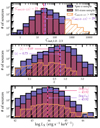 |
Fig. 1. Distribution of 1.0 − 2.3 keV net counts (top panel), spectroscopic redshifts (middle panel), and 2 keV monochromatic luminosity LX (bottom panel) for our spec-z (purple filled), BH-mass (red filled), and over-bright sources in the spec-z sample (orange hatched), respectively. The median value for spec-z (BH-mass) sample is marked with purple dashed (red dashed) lines. |
We refer to the final sample as the “BH-mass” sample. By construction, our “BH-mass” sample is constituted of only bright, broad-line type 1 AGNs. The X-ray spectra are dominated by the central AGN, and should have negligible contamination from the host galaxy (XRB) or the CGM (hot gas). The NUV completeness is ∼93% (compared to the SDSS optical counterparts) and thus acceptably high. We systematically evaluate the potential selection biases from NUV incompleteness and redshift-dependent effects in Appendix B.3, and confirm that they do not significantly affect the primary conclusions in this work.
The requirement of SDSS-measured BH mass reduced our sample size sharply from ∼28k to ∼5k sources. For some dedicated analyses that do not require BH mass, we also considered a larger sample in order to maximize the X-ray spectral quality. In our subsequent study on αox and LUV, we define a sample that skips SDSS matching, as we do not rely on BH mass. This, however, also removes the selection of type 1 AGN, and includes much fainter sources. To avoid heavily obscured (type 2) AGN in this sample, and to avoid low redshift galaxies with XRB dominating the X-ray emission, we additionally perform a luminosity cut in 2 keV LX > 1 × 1042 erg s−1 keV−1 and UV luminosity (ν Lν)UV > 3.16 × 1043 erg s−1 (see Section 2.4 below for our derivation of UV and X-ray monochromatic flux), the boundary chosen to match our BH-mass sample. The resulting larger sample, containing 17 929 sources, is called the “spec-z” sample in the sections below.
Not all type 1 AGNs are unobscured – and some of them can even be mildly or even heavily obscured (NH ≳ 1 × 1022 cm−2), especially for a hard X-ray selected sample (e.g., Waddell et al. 2024; Nandra et al. 2025). However, as can be seen in Section 5, our stacked spectra are typically smooth and devoid of significant absorption features (nH < 5 × 1020 cm−2), suggesting that the influence from neutral absorption on our (soft X-ray selected) sample should be small in general. However, we do refer readers to Section 7.5 for a more detailed discussion on caveats and cautions regarding the absorption issues during stacking.
In Fig. 1 we present the distribution of rest-frame 1.0 − 2.3 keV net photon counts Cnet, 1.0 − 2.3 (top), redshift z (middle), as well as the 2 keV monochromatic luminosity LX (bottom) for our sample. On average, our spec-z sample (purple histogram) has a median Cnet, 1.0 − 2.3 of 28, z of 0.73 and LX of 43.92, close to our BH-mass sample (red histogram) with median Cnet, 1.0 − 2.3 of 23, z of 0.69 and LX of 43.92. As a comparison, we also plot the over-bright sources (defined as Cnet, 1.0 − 2.3 > 400), which are dropped in sample selection. Typically, these sources have lower redshift as compared to BH-mass or spec-z sample.
2.2. Mass and Eddington-ratio subgroups
The AGN optical-UV spectral shape is sensitive to BH mass and Eddington ratio, so it is crucial to stack sources with similar MBH and λEdd when later considering stacked optical-UV data. Based on our BH-mass sample, we create a 3 × 3 grid on the MBH − λEdd plane, as shown in Fig. 2. In each grid bin, we stack data of all sources. The log λEdd binning edges are [ − 2.0, −1.34, −0.67, 0], while the log MBH binning edges are [8.0, 8.5, 9.0, 9.5].
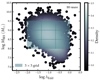 |
Fig. 2. Distribution of MBH and λEdd of our BH-mass sample, with color mapping density. The 3 × 3 MBH-λEdd grid is shown as blue transparent boxes. |
While stacked X-ray data should be safely AGN-dominated, this is not necessarily true for the stacked UV data. Especially the lowest λEdd bin with the highest MBH can be contaminated by UV-luminous star formation, and we do see the stacked UV spectra are very blue (Fig. 8). With the assumption that the galaxies are on the main sequence (following Popesso et al. 2023) with a galaxy stellar mass 200 times that of the BH mass (Kormendy & Ho 2013), we estimate with a simple stellar population model (using GRAHSP, Buchner et al. 2024) NUV fluxes up to approximately 200 μJy for these two bins (see Appendix C for details), which is near the median observed fluxes in those bins. While the actual contamination may be much lower if the fraction of star-forming galaxies is small, we are cautious on the interpretation of the two bins at log λEdd < −1.5 and MBH > 108.5 M⊙. We do not consider these further in later discussion.
2.3. eROSITA spectra extraction
At our sample X-ray positions (both “BH-mass” and “spec-z” sample), we extract spectra from all five eROSITA all-sky surveys. This gives the deepest exposure possible, and over 4 times more counts than the first all-sky survey alone. The source and background spectral extraction is described in Merloni et al. (2024). Briefly, we feed the eROSITA pipeline code srctool with the calibrated event files and source coordinates. srctool automatically determines the optimized source and background regions, within which the source and background spectra are extracted. Ancillary response files (ARF) are extracted from the same region as the corresponding sources, and corrected for vignetting (CORRVIGN) and PSF loss (CORRPSF). The response matrix files (RMF) are also extracted, but are in fact identical among all sources, since no in-orbit calibration for RMF has been taken for the moment.
eROSITA consists of seven telescope modules (TMs). For TM 5 and 7, there exists a potential light leak issue due to the lack of an on-chip optical filter on the CCD (e.g., Predehl et al. 2021), which is most pronounced below ∼0.3 keV and non-negligible for soft X-ray emission line studies. For our study focusing mainly on the continuum above 0.3 keV, this issue should be less severe. Therefore, to improve the spectral counts we simply utilize all seven TMs. We verified that removing TM 5 and 7 did not affect our main results.
The extremely high photon counts in the eROSITA stacked spectrum allow the hard X-ray power law, and thereby the soft “excess”, to be constrained. The signal-to-noise ratio is high, even at the hard X-ray band. For our “BH-mass” sample with 4159 sources, we obtain total exposure time of 3 Ms and total photon counts of 3.7 × 10⁵ within the rest-frame 0.2 − 10 keV band (7 × 10⁴ within rest-frame 2.3 − 8.0 keV). For the larger “spec-z” sample, the total exposure time is 23 Ms with 2.1 million photon counts (4.5 × 10⁵ within rest-frame 2.3 − 8.0 keV), likely exceeding any existing stacking experiments on AGN.
2.4. Luminosity measurement
To better characterize our sample, we estimate the X-ray (LX) and UV (LUV) monochromatic luminosity for each source. Due to the complex response, the X-ray monochromatic flux (erg s−1 cm−2 keV−1) or luminosity (erg s−1 keV−1) cannot be converted trivially from the Pulse Invariant (PI) spectrum (Counts s−1 keV−1), and has to be combined with spectral fitting. Therefore, to derive the rest-frame 2 keV monochromatic luminosity LX (erg s−1 keV−1), we follow a procedure similar to Liu et al. 2022 using XSPEC (Arnaud 1996). Briefly, different models are applied to unfold the spectra, depending on the 0.2 − 2.3 keV net counts. If the net count is greater than 20, we adopt an absorbed power law and blackbody model (TBabs*zTBabs*(zpowerlw+zbbody) in XSPEC notation) on the 0.2 − 8.0 keV band. All parameters are optimized except for the Galactic absorption column density of TBabs, which we fix to the NH, Gal of each source3. When the number of counts is greater than 10, we adopt the model TBabs*zpowerlaw on the 0.4 − 2.2 keV band, fitting for the normalization and photon index. For the remaining cases with poor spectral quality, we fix the photon index at 2 and fit only for the normalization. For all cases, we read the best-fit rest-frame 1.999 − 2.001 keV model luminosity with XSPEC command lumin, and convert it into 2 keV monochromatic luminosity via  .
.
To measure the intrinsic UV monochromatic luminosity, we first perform Galactic extinction correction and K-correction on the NUV monochromatic flux. We assumed a power-law SED (Fν ∼ να) and spectral index α = −0.65 (Natali et al. 1998; choosing a MBH-λEdd-dependent α would not alter our results, see Appendix B.2) applicable to AGNs within 1200−5100 Å range:
 (1)
(1)
where we took R = R(NUV) = 7.95 (Bianchi et al. 2017, for Milky Way-type dust) and calculated E(B − V) from the extinction map of Schlegel et al. 1998 based on the RA and Dec of each source. For some high-z sources (e.g., z > 1), the adopted spectral index may not be applicable, as the rest-frame NUV would shift below 1200 Å (the lower bound of Natali et al. 1998) and IGM absorption would be stronger. Nevertheless, the impact should be minor as the high-z fraction is small. Analysing only a low-z sample also did not change our results (see Appendix B.3 for discussion). We then converted the rest-frame NUV monochromatic flux into the rest-frame 2500 Å monochromatic flux, assuming the same UV SED slope. Finally, the monochromatic flux was multiplied by 4πdL2 to derive the UV monochromatic luminosity at 2500 Å (LUV, erg s−1 Hz−1), where dL is the luminosity distance.
In order to characterize the relative importance of X-ray to UV, we adopted the “X-ray loudness” parameter αox, defined as the point-to-point slope between 2 keV and 2500 Å on luminosity (erg s−1 Hz−1) diagram (e.g., Avni & Tananbaum 1982):
 (2)
(2)
Here, the unit of LX has been converted from erg s−1 keV−1 to erg s−1 Hz−1 to match that of UV. We note that following Sobolewska et al. 2009, we applied an additional minus sign to keep αox positive. The stronger the X-ray luminosity is compared to the UV luminosity, the smaller the value of αox would be.
The luminosity measurements come with uncertainties. For our BH-mass sample (similar for spec-z sample), the median 68 % uncertainty in log LX is ∼0.14 dex, while the photometric uncertainty in log LUV is ∼0.13 dex. After propagating these errors, the median uncertainty in αox is ∼0.075. Notably, these uncertainties for individual sources remain nearly half as small as the typical bin size of each subgroup (∼0.34 dex for each of the 3 LUV subgroups, and ∼0.14 dex for each of the 3 αox subgroups). Therefore, they are unlikely to significantly impact our later conclusions involving LUV or αox.
3. Methods for X-ray spectral stacking and fitting
3.1. Xstack: A novel tool for X-ray spectral stacking
Given the large number yet individually low-count nature of X-ray spectra in the era of eROSITA, a convenient and robust tool for X-ray spectral stacking sources from different redshifts is urgently needed, to support a wide range of scientific investigations. Although X-ray spectral stacking is a classical technique for improving signal-to-noise ratio and has already been applied to many scientific problems (e.g., Sanders & Fabian 2011; Bulbul et al. 2014; Liu et al. 2016, 2017; Tanimura et al. 2020, 2022; Zhang et al. 2024; Gonzalez Villalba 2024), certain technical limitations still exist. These include, how to optimally preserve spectral shape when stacking sources with different redshifts and fluxes; how to properly account for Galactic absorption during stacking to recover the intrinsic extragalactic spectra; and how to perform statistically sound spectral fitting on the stacked result.
To address these issues, we develop Xstack, a standalone pipeline for X-ray spectral shifting and stacking. Briefly, Xstack first sums all (rest-frame) PI spectra, without any scaling; and then sum the rest-frame corrected full responses (ARF*RMF), each with appropriate weighting factors to preserve the overall spectral shape.
The more technical aspects of Xstack are presented in Appendix A, beginning with a pedagogical review of basic concepts in X-ray spectroscopy. Here, we highlight the key features of the code:
-
Preservation of spectral slope, achieved by properly assigning weighting factors to each response (ARF*RMF) during the stack;
-
Correction for Galactic absorption, by applying a NH, Gal-dependent Galactic absorption profile (TBabs) to each ARF before shifting and stacking (see also Zhang et al. 2024);
-
Well-defined statistics for subsequent spectral fitting, due to the preservation of Poissonian nature of the data. The stacked background is approximated with a Gaussian distribution.
In Appendix B.1, we also validate our code’s ability to preserve spectral shapes through simple power law simulations.
3.2. X-ray spectral fitting: Global settings
The correct propagation of uncertainty allowed us to perform spectral fitting on the stacked PI spectrum, combined with the stacked response. Each stacked spectrum considered is analyzed within the 0.3 − 8.0 keV band. Below 0.3 keV, we find that only ≲20% sources contribute to the rest-frame stacked spectra (≲30% sources contributing to the rest-frame stacked ARF), potentially leading to an insufficient sampling of ARF and background data; while above 8 keV we find that the background contribution is higher than ∼90% and does not provide much information. Since our data follow the Poisson distribution while the scaled sum of backgrounds approximates the Gaussian distribution, we adopt the PG statistic4. The parameter confidence regions are derived from the 100 bootstrapped stacked spectra fit, which accounts for both Poisson fluctuation and sample variance.
3.3. Phenomenological spectral model
To characterize the strength of soft excess in model-independent way and compare with literature, we first apply a phenomenological rest-frame model, which can be written as TBabs*(powerlaw+cutoffpl+gauss) in XSPEC terminology. We now describe the components of this model in turn.
The hard X-ray primary continuum is modeled by a powerlaw, N = A × E−ΓPC5, with the photon index ΓPC set within a relatively narrow range 1.7 − 2.3, because (1) from a data-driven point of view, the hard X-ray spectral index of our stacked spectra in Fig. 4 do not deviate much from 2, and we want to prevent the rare case where an unphysically hard (ΓPC ≲ 1.5) hard X-ray primary continuum and an ultra-strong soft excess is derived from the fit; (2) the range 1.7 − 2.3 is reasonable compared with literature (e.g., Nandra & Pounds 1994; Brightman et al. 2013), given the median physical quantity of each αox/LUV/λEdd/MBH subgroup. A Gaussian component gauss is also included to account for the iron line at ∼6.4 keV, but since it is not the major focus of this study, we simply fixed the line centroid at 6.4 keV and sigma at 0.019 keV (e.g., Shu et al. 2011).
A cutoff power law is adopted to model the soft excess. The spectral model is N = A × E−ΓSEexp(−E/Ecut), with the photon index ΓSE set to be softer than ΓPC by at least 0.5 (ΓSE − ΓPC > 0.5), and the cutoff energy Ecut set below 2 keV. The former setting is to ensure a physically interpretable result, while the latter setting is motivated by observed soft excess spectra showing a bend-over at high energies (Fig. 5). Furthermore, if the soft excess component is a “warm corona” structure with typical temperature within 0.1 − 1.0 keV (e.g., Petrucci et al. 2018), its spectrum is approximately a cutoff power law with the cutoff energy Ecut by a factor of  lower than the temperature. Following the standard in literature (e.g., Boissay et al. 2016), we also measured the strength of the soft excess component, defined as the luminosity ratio of soft excess to primary continuum within the 0.5 − 2.0 keV band:
 (3)
(3)
Finally, all the above components are absorbed by an intrinsic absorption layer (TBabs). The column density nH is allowed to vary between 0 and 10 × 1020 cm−2, a reasonable range for optically unobscured AGN (e.g. Ricci et al. 2013). We tested the disnht model (Locatelli et al. 2022), which allows for a log-normal distribution of column densities, but the standard deviation parameter is difficult to constrain when a soft excess component is also modeled.
4. Methods for UV stacking
4.1. UV photometry stacking
For a panchromatic understanding of the underlying physics, it is necessary to combine UV data in spectral fitting, and apply a more physical model.
To that end, we stack the GALEX NUV, SDSS u and g (Abazajian et al. 2009) photometry for each source, after galactic extinction correction (we take R(u) = 4.24, R(g) = 3.30 from Schlafly & Finkbeiner 2011) and K-correction with the same assumption as in Section 2.4. That means for a source with z = 0.5, its NUV flux with central wavelength at 2135.7 Å will still contribute to a data point at 2315.7 Å in the stacked spectrum, rather than at rest-frame wavelength 2315.7/(1+0.5) = 1543.8 Å. We do not stack the rest-frame flux directly, due to (1) in the energy range where both SDSS and GALEX contribute, the SDSS signal will completely dominate over GALEX, as SDSS has much larger effective area than GALEX; (2) because we are stacking discrete UV photometry with relative narrow wavelength range compared to redshift distribution, the overlapping region for different sources on the rest-frame energy grid will be small, leading to an overall small completeness in each energy bin; (3) for high redshift sources contributing to the rest-frame EUV, their stacked spectrum is severely biased due to IGM distortion. Additionally, we note that using a MBH-λEdd-dependent UV SED slope for K-correction does not significantly affect our later AGNSED fit, with changes in the best-fit parameters remaining within 1σ.
We now have many individual UV photometry points anchored on energies corresponding to g (2.6 eV), u (3.5 eV) and NUV (5.4 eV). Since the effective areas for each energy bin do not vary significantly from source to source, we sum the flux in each energy bin. To ensure that the stacked UV spectrum can be compared with stacked X-ray spectrum, we divide the entire stacked UV spectrum by the X-ray response normalization factor (∑lWl in Appendix A.3).
Photometry often comes with calibration issues (e.g., Arnouts & Ilbert 2011; Bianchi et al. 2017), which cannot be improved by stacking. Moreover, some systematic issues (e.g., IGM absorption, and uncertainty of K-correction) degrade the reliability of our UV data. Therefore, we followed the standard practice of SED fitting procedure by accounting for these extra uncertainties as η fraction of stacked flux (Fg/u/NUV), and we added them in quadrature in addition to the original uncertainty (σg/u/NUV) propagated from the catalog:
 (4)
(4)
In practice, η is chosen as 1.5% for g and u band. For NUV, we conservatively choose a value as large as 30% (e.g., Georgakakis et al. 2017), as the calibration and systematic issues are generally more severe in GALEX. Finally, we note that decreasing the statistical weight of UV data in UV-Xray linked spectral fitting could also prevent the UV data (typically with smaller uncertainties compared with X-ray) from dominating the fit.
At the end of each bootstrap, we also added additional random scatter to the data (not only the error bar) with an amplitude corresponding to η fraction of stacked flux in order to account for the systematic issues.
4.2. Physical spectral model: AGNSED
We fit our optical-UV X-ray stacked data with the physical model AGNSED (Kubota & Done 2018). In this model, the accretion disk is radially separated into three regimes. For a given BH mass and Eddington ratio, the standard Novikov-Thorne emissivity profile (Novikov & Thorne 1973) is assumed for the accretion disk, which extends as far as Rout. At each annulus, the emergent spectrum is in the form of blackbody. Below the radius RWC, the Compton scattering in the disk surface becomes dominant, and the disk transits into a “warm corona”, which is modeled by a Comptonized component (nthcomp) with photon index ΓWC and hot electron temperature kTWC. The seed photon temperature, on the other hand, varies with radius and is tied to the local underlying disk temperature. Going further down to RHC (RHC < RWC), the “warm corona” or disk is believed to truncate, forming a “hot corona” with completely different physical properties, characterized by a hot Comptonized component with a photon index of ΓHC and an electron temperature kTHC.
Our physical spectral model is written as TBabs*(agnsed+gauss) in XSPEC terminology. We fix the MBH (λEdd) at the sample median value of each bin. For the warm corona, we allowed ΓWC to vary between 2.25 and 5, and kTWC from 0.1 − 1.0 keV. For the hot corona, we fix kTHC at 100 keV, while allowing ΓHC to vary between 1.7 and 2.3 for the same reason as in Section 3.3. Following Hagen et al. 2024b, we fix Rout at 104Rg (gravitational radius,  ), BH spin a* at 0.0, cosine of inclination angle at 0.87 (as the sources are type 1), and hot coronal height at 10 Rg. Other parameters of AGNSED, including RWC and RHC, are allowed to vary freely. For the intrinsic absorption TBabs and iron line complex gauss, we adopt a similar setting as in Section 3.3.
AGNSED is an energy-conserving model, and for fitting individual sources (rather than the stacked spectrum), its normalization is typically fixed at 1, with the distance set to the physical value corresponding to the source redshift. However, due to the nature of our stacking (which preserves spectral shape rather than absolute normalization), and since we are primarily interested in the spectral shape, we adopted an arbitrary distance and allowed the normalization to vary freely. We note that this approach is only valid when stacking sources with similar MBH and λEdd (and thus comparable luminosities), as is the case for our BH-mass sample in Section 6.
5. Phenomenological modeling of stacked X-ray spectra
5.1. Full sample results
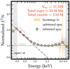 |
Fig. 3. Summed eROSITA spectrum from 23 Ms of observations (“spec-z” sample). To reveal the intrinsic spectral shape of AGN, the spectrum is divided by the ARF and multiplied by E2 (so the unit proportional to keV2 Counts cm−2 s−1 keV−1 or erg cm−2 s−1), normalized at 4 keV. The gray points are the unbinned data, while yellow circles show a logarithmic rebinning. The yellow shaded area, derived from bootstrapping the sample for 100 times, indicates the 68% uncertainty range of the spectrum from both stacking process and Poisson fluctuation (the plotting routine also applies to Figs. 4–8). Only the spectrum between 0.3 keV and 8 keV is used in this work. Between 1 and 6 keV, the spectrum is approximately linear in this log-log plot, while below, the spectrum bends upwards. Between 6 and 7 keV, a bump is visible despite the relatively larger errorbars. Power laws of typical photon indices are plotted only for visual comparison. |
In Fig. 3, the stacked spectrum of 17 929 sources from our largest spec-z sample is presented. The spectrum is smooth and appears bent upwards towards the soft end. To reveal the intrinsic spectral shape unaffected by the varying effective area and channel energy width across the whole energy band (0.2 − 10 keV), the plot shows the stacked spectrum divided by the effective area (from the stacked ARF) and energy width of each channel. Since we want to highlight the “soft excess” from the underlying hard X-ray power law (with a typical photon index of ∼2), we multiply the spectrum by the energy squared to obtain units of keV2 Counts cm−2 s−1 keV−1 (E2N). Finally, as we are not interested in the absolute normalization for this visualization, we renormalize the resulting “ARF-weighted” spectrum at 4 keV, where the hard X-ray power law dominates, shown as gray points in Fig. 3 (“unbinned spec”). For clarity, we also rebin the spectrum on a logarithmic energy scale, as shown by the yellow-filled circles (“rebinned spec”). The uncertainty range of the rebinned stacked spectrum, resulting from both stacking process and Poisson fluctuation, is computed by 100 bootstraps, which randomly leave out spectra from the sample. This is shown as the yellow shaded area in Fig. 3. Since both the number of sources and the number of photon counts are very large, the uncertainties are very small. Because bootstrapping error bars are sensitive to the heterogeneity of the sample, finding small error bars indicates a similar spectrum within the stacked sample.
Several notable features are apparent in the binned spectrum in Fig. 3. Between 1 keV and 6 keV, a primary power-law component with a photon index of ∼2 is evident. This is typical for AGN and consistent with the average value observed in eFEDS sources (Liu et al. 2022). Considering the continuation of this power law, below ∼1 keV a prominent soft excess component is present. This is explored in greater detail in later sections. Additionally, an iron line feature is observable around ∼6 − 7 keV. Such a component, generally unexpected for single-source spectrum due to eROSITA’s poor effective area above ∼2 keV, appears in both the unbinned and rebinned ensemble stacked spectrum. This demonstrates the power of spectral stacking. This iron line feature cannot be attributed to the background, because the background iron lines (e.g., Predehl et al. 2021) arising at z = 0 are blurred and dissolved as we rest-frame shift the source and background spectra.
5.2. Differences in physical subgroups
To investigate the variation of spectral profile with different physical properties, we divide the sample into three equally populated subgroups according to different physical quantities (αox, LUV6, λEdd, MBH), and stack sources in the same subgroup. The αox and LUV binnings are based on our “spec-z” sample, containing ∼5976 sources in each subgroup, while the λEdd and MBH binnings are based on the “BH-mass” sample, containing ∼1390 sources in each subgroup. The resulting spectra normalized at 4 keV, as shown in Fig. 4, facilitates a pure data-driven analysis on the evolution of soft excess. We note that the αox- or LUV-binned spectra remain similar when stacking the “BH-mass” sample.
We first uncover significant trends in Fig. 4 that the soft X-ray spectrum (≲2 keV) becomes stronger compared to hard X-ray for increasing αox (first panel) and λEdd (third panel), aligning well with previous studies (Walter & Fink 1993; Grupe et al. 2010, and Fig. 14 from a similar stacking work, Jin et al. 2012a), and extending these results to a larger population. In these two panels, the difference between stacked spectra is much larger than the uncertainties, which are often too small to be seen. For the LUV binning (second panel), the trend is weaker, and a small difference is only apparent between the brightest subgroup and dimmest subgroup. In the right-most panel, the trend for MBH is reversed. Less massive sources have steeper soft X-ray spectra than more massive sources, in agreement with previous studies (e.g. Porquet et al. 2004; Piconcelli et al. 2005).
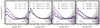 |
Fig. 4. Stacked spectra in three equally sized groups (colored lines) divided by αox, LUV, λEdd, and MBH (panels from left to right). The legend gives the mean value of each subgroup. Error bars are obtained with bootstrapping as in Fig. 3, but are generally very small except above ∼8 keV. In the left panel, the three colored lines are indistinguishable above 2 keV. Below 1 keV, the blue data points from the lowest αox subsample are always below the pink points from the highest αox subsample. The λEdd panel shows an even larger spread between subgroups, while it is less pronounced in the LUV panel and reversed in the MBH panel. |
We present in Fig. 5 the difference spectrum between the highest αox and lowest αox subgroup from Fig. 4. The y-axis value indicates the strength of residual flux (E2N) relative to hard X-ray power law at 4 keV. The significant residual in the soft X-ray (10 − 100% that of hard X-ray power law at 4 keV) alongside the much weaker residual in the hard X-ray power law, explicitly demonstrates that the soft excess cannot arise from reflection alone, unless the efficiency of hard X-ray power law producing soft excess (e.g., the geometry) changes drastically with αox. The difference spectrum in Fig. 5 also reveals the intrinsic soft excess as a power law between 0.3 and 1 keV, where it starts to be “cut off”, decreasing below the power law by an e-fold at approximately 2 keV.
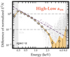 |
Fig. 5. Difference spectrum between the highest and lowest αox subgroups from the left panel of Fig. 4 highlighting the spectral shape of the emerging soft excess component. The binned yellow data follow a line in this log-log plot corresponding to a Γ = 3.2 power law (dashed purple line), but fall below beyond 1 keV. The horizontal lines mark where the flux (E2N) of the difference spectrum amounts to 100%, or 10% of the original normalized spectra at 4 keV, where the spectra are normalized. The yellow data points are above the 1x line below 0.5 keV, and below the 0.1x line above 2 keV. Above 3 keV, the difference falls below 1%. |
Overall, the hard X-ray spectrum (≳2 keV) of Fig. 4 is more stable than the soft X-ray band. This is the case across different subgroups for all binnings, except that we find the lowest MBH subgroup does seem to have the steepest hard X-ray power law. However, the spectral quality in this regime is also relatively poor, inhibiting direct interpretation from data and requires further spectral fitting, which is presented in the next section.
5.3. Phenomenological spectral fits
Motivated by the apparent differences in spectra, such as Fig. 5, we quantified the strength of the soft excess. We present in Fig. 6 (for the αox and LUV binnings) and Fig. 7 (for the λEdd and MBH binnings) the best-fit total model from a single fit (thick black line), as well as different best-fit components after 100 bootstrap experiments (green lines for soft excess, and blue lines for hard X-ray primary continuum). The distribution of the bootstrap realizations provide a clear view of parameter uncertainties as well as degeneracies. The source number, as well as fitting statistics are stated in each panel. Each panel also states the measured soft excess strength q. We use this to find the physical variable that causes the largest change in q.
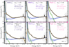 |
Fig. 6. Fits to stacked spectra (from “spec-z” sample) in equally sized bins of αox (top panels) and LUV (bottom panels). The legend gives the mean value of each subgroup, the number of stacked sources, and the fitting statistics. The soft power law (green) and the hard power law (blue) as well as the sum (black) are shown. Each curve is the best fit to a bootstrap realization of the sample. In the top panels, from the left to right panels, the green curves move upwards. The strengthening of the soft excess is quantified by q with error bars, increasing from 0.13 to 0.58. The bottom panels show fewer changes in the green warm corona component with LUV. |
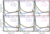 |
Fig. 7. Similar to Fig. 6 but for λEdd (top panels) and MBH (bottom panels) using the “BH-mass” sample. In the top panels, from the left to right panels, the green soft excess component curves move upwards, and the soft excess strength, q, increases from 0.13 to 0.52. |
Overall, our phenomenological model yields an acceptable fit, mostly with the PG statistic per degree of freedom (d.o.f.) smaller than 1.207. For the “High LUV” subgroup, the fit is rather poor (PG stat/d.o.f. = 1.32), along with a high nH value (pegged at the upper bound 10 × 1020 cm−2). We consider this as a data problem arising from the relatively small number of sources effectively contributing to the 0.3 − 0.4 keV band, as the highest luminosity subgroup contains more high-redshift sources than the lower luminosity subgroups. Indeed, when ignoring 0.3 − 0.4 keV, the fitting statistic becomes much better (from 1.32 to 1.07) and NH ∼ 0.66 × 1020 cm−2, indicative of an unobscured spectrum, becomes more reasonable.
The strong variation of the soft excess strength q and αox or λEdd, as shown in Fig. 4, is now quantitatively confirmed. The soft excess is equivalent to approximately 10% of the hard X-ray primary continuum flux in the 0.5 − 2.0 keV band at the lowest αox or λEdd subgroup, increasing to approximately 50 − 60 % at the highest αox or λEdd subgroup. That is, the soft excess luminosity increases by a factor of five relative to the hard power law. The trend is weaker for LUV and log MBH, with soft excess strength staying close to ∼0.30 for each subgroup.
Table 1 lists the spectral fit parameter values. This includes their best-fit values as well as 68% uncertainties from different physical subgroups of Ecut, ΓSE, ΓPC and NH. The median αox, log LUV, log λEdd or log MBH for each subgroup are also included in parentheses on the third row. For Ecut, we find a tentative positive correlation with αox, and a relatively strong correlation with LUV. Most subgroups require a relatively flat soft excess with ΓSE ∼ 2.68, and no significant trend can be found neither except for the LUV binning. We also did not find significant evolution for ΓPC, despite the “low MBH” subgroup exhibiting a softer value ( ) than average. Overall, the absorption is mild, typical for type 1 AGNs and consistent with our assumption. A further discussion on the above trends is presented in Section 7.
Spectral fitting results for the phenomenological model of different αox, LUV, λEdd or MBH binnings.
Spectral fitting results for the physical model (AGNSED).
6. Multiwavelength modeling with AGNSED
Our spectral binning by either MBH or λEdd (Section 5.3) may potentially introduce selection effects due to the flux-limited nature of our sample. Specifically, the lowest (highest) λEdd bins preferentially contain sources with the highest (lowest) MBH, as shown in our Fig. 2 and also discussed in Section 6.1 of Jin et al. 2012a. Also physically, we would like to tease out how the accretion disk and warm corona change with λEdd and MBH behind the observed trend of soft excess, using the physical AGNSED model. We therefore constructed the optical-UV X-ray SED for our BH-mass sample on the 3 × 3 MBH-λEdd grid (Fig. 2) following the stacking method described in Section 4.1.
In Fig. 8, we present the optical-UV X-ray SED on our 3 × 3 MBH − λEdd grid, overlaid by best-fit bootstrap folded models. The source intrinsic models (absorption corrected) are shown in Fig. 9. Generally, a stronger soft excess (q) and a larger UV to X-ray ratio (αox) can be seen along the x-axis (increasing λEdd). Along the y-axis (increasing MBH), the soft excess tentatively becomes weaker, and no significant trend can be seen for the UV to X-ray ratio. Interestingly, the NUV-u slope also seems to be steeper for increasing λEdd, and flatter for increasing MBH, except for the two low λEdd – high MBH (top two bins in the first column) with relatively strong star-forming contamination. We note that these UV trends appear, even when we assume a constant UV SED slope (rather than a λEdd or MBH-dependent slope) for K-correction, and should therefore be genuine.
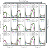 |
Fig. 8. Optical-UV X-ray SED on our 3 × 3 MBH-λEdd grid overlaid by best-fit bootstrap models, with red for disk (DK), green for warm corona (WC), and blue for hot corona (HC). The legend gives the source number, median MBH, λBH, best fitting statistic in each bin. A toy model illustrating the disk-corona size (warm corona radius RWC, hot corona radius RHC, both in units of Rg) is shown on the top right of each panel. We note the potential star-formation contamination in two upper-left bins with low λEdd – high MBH when interpreting the results. |
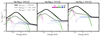 |
Fig. 9. Best-fit AGNSED models for our 3 × 3 MBH-λEdd grids (excluding the two with potential star formation contamination). Different components are shown with the same color convention as in Fig. 8. As no data are involved, we scaled the y-axis to physical values (erg s−1) by setting the AGNSED distance parameter as dL = 100 Mpc and the normalization to 4πdL2. |
The physical meaning behind these trends in the model can also be considered. In the top right corner of each panel in Fig. 8, an illustration of the disk-corona model geometry is shown, where the transitional radii of RWC and RHC are scaled to real values. More quantitatively, we present in Fig. 10 the evolutionary trend for RHC, RWC and log(RWC2 − RHC2) (the “size” of the warm corona relative to the hot corona), as a function of λEdd and MBH. We label the bootstrap median as well as 68% range for each value. The color map is linearly interpolated for visualizing trends. The low λEdd – high MBH bins are grayed out for star-forming contamination (see Section 2.2). For the remaining bins, as λEdd increases, RHC becomes smaller, and RWC increases, indicating that the warm corona increases in relative size. On the other hand, as MBH increases, RHC remains relatively constant, while RWC decreases, indicating a smaller warm corona.
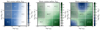 |
Fig. 10. Evolutionary trend of the hot corona radius RHC (left), warm corona radius RWC (middle), and warm corona “size” log(RWC2 − RHC2) (right) on the 3 × 3 MBH-λEdd grid. The color is linearly interpolated for visualizing trends. The two low λEdd – high MBH bins are grayed out for star-forming contamination (see text for details), except for which the warm corona radius shows a clear increasing trend with increasing λEdd and decreasing MBH. The hot corona radius decreases with increasing λEdd while remains constant for different MBH. |
The coronal radius evolution and our pure data-driven analysis of spectral shape are consistent. Since most of the X-ray photons are emitted from the hot corona, in the AGNSED model the hot corona radius reflects the relative importance of X-ray to total luminosity (∼αox). The negative correlation between RHC and λEdd simply manifests that αox increases with λEdd. The warm corona radius, on the other hand, is more complex and relies on both UV and soft X-ray. First, RWC is related to the outer edge warm corona seed photon temperature, which peaks at UV and is determined from NUV-u slope. Second, since a larger warm corona produces more soft X-ray emission relative to the hard X-ray primary continuum (hot corona), RWC should also be related to the soft excess strength q, defined as the ratio of soft excess to hard X-ray primary continuum (in the most extreme case, if there is no soft “excess”, then there should be no warm corona). In our case, the RWC increase (decrease) with λEdd (MBH) is generally consistent with the observational trend that q and NUV-u slope increases (decreases or remains constant) with λEdd (MBH) in Fig. 8.
No significant trends are found aside from RHC and RWC (Table 2). The warm corona photon index ΓWC is found between 2.25 ∼ 3, and tentatively becomes steeper for increasing λEdd. For the hot corona photon index ΓHC, we find that its correlation with λEdd is rather weak for higher BH masses (log MBH ∈ [8.5, 9.5]). ΓHC generally becomes larger for lower BH masses (log MBH ∈ [8.0, 8.5]), and a positive correlation between ΓHC and λEdd is revealed. Finally, the majority of intrinsic absorption column density nH consistently fall below 10 × 1020 cm−2. We originally found the nH at the highest MBH – highest λEdd (equivalently highest luminosity) bin pegged at 10 × 1020 cm−2. For the same reason as Section 5.3, we ignore 0.3 − 0.4 keV, and find that nH returns to a more realistic value of ∼5 × 1020 cm−2.
7. Discussion
In this section, we compare our results with the literature and discuss the physical implications for the disk-corona connection. We first discuss some phenomenological properties of the soft excess and the relation with UV for insights on the soft excess origin (Section 7.1). Then, we focused on the disk radial structural change as implied by our data, starting from the standard outer disk to disk transition into the warm corona (Section 7.2) and further toward disk truncation into the hot corona (Section 7.3), assuming the configuration of AGNSED. With our stacked optical-UV X-ray spectra, we also discuss in Section 7.4 the bolometric corrections as a function of many physical parameters. Finally, in Section 7.5, we discuss some caveats of our study.
7.1. The connection between UV and soft excess
The physical origin of the soft excess has long been debated. In current understanding, either it originates from the inverse Compton scattering of disk UV photons (e.g., Petrucci et al. 2013, 2018), where it is more related to UV (disk) than hard X-ray (hot corona); or it could possibly be the blended reflection feature of hot corona illuminating on the inner ionized disk (e.g., Ross & Fabian 1993; Crummy et al. 2006), where it should show stronger dependence on the hard X-ray rather than the UV. Although both components can contribute to the real observed soft excess (e.g., Chen et al. 2025), the warm corona contribution has been proven to dominate by many recent studies, either by model comparison (e.g., Waddell et al. 2024) or directly measuring the fraction of warm corona to ionized reflection (e.g., Ballantyne et al. 2024).
We investigate the response of the soft excess by stacking X-ray spectra on groups of similar AGN parameters. Stacked spectra in groups of different αox (left panel of Fig. 4, top panel of Fig. 6) show that, as the disk becomes stronger compared to the hard X-ray, the soft excess responds accordingly while the hard X-ray spectral profile (both the hard X-ray power law and the iron line at ∼6.4 keV which is indicative of the reflection feature) remains nearly unchanged. This trend supports the dominance of warm corona over ionized reflection in two ways. First, in the reflection scenario, the soft excess originates from hard X-ray reflecting off the inner accretion disk; a constant hard X-ray spectrum would therefore predict a relatively stable soft excess strength q, yet we now observe that a fivefold amplification of q (Fig. 4). Second, αox quantifies the relative strength of the UV (where UV photons serve as seed photons for the warm corona) to X-ray, and we see that q closely tracks the increase in αox. We note that the strong correlation between soft excess strength and αox has also been reported in ROSAT AGN sample studies (e.g., Walter & Fink 1993). Regarding αox and hard X-ray photon index ΓPC, previous studies involving large AGN samples from Chandra across a wide redshift range 0.1 − 4.7 (e.g., Kelly et al. 2007; Sobolewska et al. 2009) also do not show a strong correlation. Several XMM-Newton studies of nearby bright Seyfert 1 galaxies do reveal a weak correlation between ΓPC and αox (Jin et al. 2012a, and Chen et al., in prep). Whether the discrepancy arises from instrumental calibration (especially in the hard X-ray) is still unclear, and is postponed to a future study involving stacking XMM-Newton or Chandra sources. Nevertheless, we note that the correlation reported in Jin et al. 2012a is at most marginal (p = 0.01), and from the three αox-binned stacked optical-UV X-ray SED (their Fig. 14) ΓPC also changes only by ∼0.1. The correlation between ΓPC and αox in Chen et al. in prep is much weaker than that between soft X-ray slope and αox (similar to this work). Therefore, our conclusions should remain largely consistent with previous studies.
In a flux-limited survey, αox is correlated with LUV, so we should also anticipate a correlation between q and LUV. As seen in Fig. 4 and lower panel of Fig. 6, such a trend does exist in our data, but is nevertheless weaker than the correlation between q and αox. Therefore, it is possible that the soft excess strength is intrinsically related to the relative power of UV in the total light, and the correlation between q and absolute UV luminosity is just a secondary effect, due to the αox ∼ LUV relation. This might suggest that AGNs across different luminosities share the same X-ray spectral shape and can interestingly be linked to the finding that AGNs across different luminosities share the same optical-UV SED (e.g., Cai & Wang 2023; Cai 2024). Despite this, we interestingly find in the stacked spectra that (Table 1), as UV luminosity increases, the soft excess photon index ΓSE increases (accompanied by an increase in cutoff energy Ecut), while the hard X-ray photon index ΓPC slightly decreases. This could possibly suggest stronger UV radiation enhances a competitive process between the soft excess component (warm corona) and the hot corona. That said, a parameter degeneracy test and a detailed treatment of the X-ray and optical selection bias are needed to validate this and will be carried out in a future study.
7.2. The disk radial structural change: From disk to warm corona
A Comptonized warm corona component can successfully explain the UV and soft excess, both in individual AGNs (e.g., Kubota & Done 2018) and stacked spectra (Hagen et al. 2024b, and our Fig. 8). However, how and why the disk transits into a warm Comptonized structure is not clearly understood.
An interesting possibility is that such a transition may relate to disk thermal instability near hydrogen ionization threshold (∼1 × 10⁴ K, e.g., Hagen et al. 2024b). Such a concept (also known as the “limit-cycle mechanism” in the literature), which was originally developed to account for periodic eruptions in dwarf novae (e.g., Mineshige & Osaki 1983; Cannizzo & Wheeler 1984), was later refined to explain AGN variability (e.g., Cannizzo 1992; Hameury et al. 2009). The basic idea is that the accretion disk hydrogen starts to be ionized at ∼1 × 10⁴ K. A small increase in temperature leads to increase in ionization and opacity, trapping more heat and thereby further increases temperature; conversely, a small decrease in temperature reduces ionization and opacity, allowing the disk to cool further. This runaway behavior leaves the disk (at critical temperature) at two extreme states, and may oscillate in between. Such a highly unstable pattern results in a disk vertical structure very unlike that of the standard slim disk (Cannizzo & Reiff 1992), and it may be the key to inducing a warm corona.
For a standard disk, the temperature Tdisk at any given radius R follows Tdisk = 6.157 × 10⁷ × (λEdd/MBH)1/4ηeff−1/4(R/Rg)−3/4 (e.g., Shakura & Sunyaev 1973; Novikov & Thorne 1973). Through AGNSED modeling, our data reveals that the warm corona radius, RWC, increases with λEdd and decreases with MBH. Inserting the median λEdd and MBH for each of the 7 grids free from star formation contamination, and assuming radiation efficiency factor ηeff = 0.1, we interesting find the disk temperature at the disk-to-warm-corona transitional radius roughly remains constant at ∼1 × 10⁴ K, with ∼0.3 dex of dispersion. We summarize this physical picture in Fig. 11.
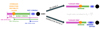 |
Fig. 11. Sketch summarizing the physical picture of disk-to-warm corona transition. A hydrogen ionization instability at ∼1 × 10⁴ K within the disk likely triggers the formation of the warm corona. For either a more massive BH or a lower Eddington ratio, the disk temperature becomes cooler, causing the transition radius (in terms of Rg) to move inward. Meanwhile, the hot corona expands (in units of Rg) as Eddington ratio decreases, to match the observed increase in Xray-to-bolometric luminosity fraction. |
The constancy of transitional temperature is consistent with Hagen et al. 2024b, although our value (∼1 × 10⁴ K) is slightly higher than theirs (∼6 × 10³ K). While 6 × 10³ K may be physically related to the hydrogen ionization change (e.g., Cannizzo & Reiff 1992), we note that a higher temperature (∼104 K) has also been found in many individual sources (e.g., Kubota & Done 2018). Moreover, there could be systematic uncertainties affecting the specific value of such a temperature (e.g., intrinsic dust extinction, potential IGM absorption), and the standard disk model may be an incomplete description of AGN accretion (e.g., Dexter & Agol 2011; Netzer & Trakhtenbrot 2014; Lawrence 2018; Antonucci 2018). Therefore, more sophisticated treatment of the host galaxy and dust extinction is needed to validate the exact temperature in the future.
Despite the potential uncertainty on the transitional temperature, the systematic transition of the disk structure could be ubiquitous across all types of AGN. Recently, Li et al. (2024) examined the disk structure of a changing-look AGN (1ES 1927+654, M ≈ 106 M⊙) at different epochs. They assume a two-zone structure, with a standard disk (producing optical-UV emission) in the outer region transiting9 into a slim disk (producing soft X-ray emission) in the inner radius, as well as a hot corona near the central BH (see their Fig. 1). This is not identical but comparable to the warm corona in our configuration. They found that the transitional radius increases at the high accretion state compared to low accretion state (see their Fig. 14), similar to the pattern observed in our Fig. 10 and Hagen et al. (2024b). Comparing 1ES 1927+654 with other normal type 1 AGNs (M ≳ 107 M⊙) at similar accretion rate, they also concluded that the transitional radius should decrease with increasing BH mass, similar to our findings in Fig. 10.
Regarding the warm corona temperature, the average we find,  , is overall comparable to other literature results (e.g., Petrucci et al. 2018; Kubota & Done 2018; Waddell et al. 2024). A slightly larger value found in Petrucci et al. (2018) and Waddell et al. (2024) could possibly be due to different energy bands or models used to constrain the warm corona. Similar to its proxy Ecut, the warm corona temperature kTWC does not exhibit significant correlation with λEdd or MBH. Our typical warm corona photon index ΓWC is consistent with other literature (e.g., Petrucci et al. 2018), and ΓWC in general shows a non-monotonous correlation with λEdd or MBH. The mild or lack of correlation between kTWC or ΓWC with λEdd or MBH is in agreement with recent findings (e.g., Waddell et al. 2024; Palit et al. 2024). This could suggest that parameters additional to accretion rate and BH mass are controlling the warm corona, such as the magnetic field, Gronkiewicz et al. (2023). Indeed, recent MHD simulation indicate the important role of magnetic field in warm corona formation as well as warm corona temperature (e.g., Igarashi et al. 2024).
7.3. The truncation of disk and the hot corona
The clear bend at ∼1 − 2 keV seen in both literature (e.g., Boissay et al. 2016) and our stacked spectra suggests the component at soft X-ray (warm corona) and hard X-ray cannot be the same structure with a continuous temperature gradient. AGNSED assumes the disk (warm corona) truncates at a radius RHC (without a physical motivation), below which the accretion flow turns into a hot Comptonized plasma, which contributes to the hard X-ray continuum.
Observationally, many works have found that the hard X-ray continuum only contributes a small fraction of the bolometric luminosity (e.g., Marconi et al. 2004; Kubota & Done 2018; Duras et al. 2020), and this fraction (the “X-ray loudness”) decreases with increasing accretion rate (e.g., Vasudevan & Fabian 2009; Ballantyne et al. 2024). This is also seen in Fig. 8, where with increasing λEdd the hard X-ray emission fraction becomes smaller in the normalized spectra. The X-ray to bolometric ratio is an important factor for constraining RHC in AGNSED (in that RHC decreases for decreasing X-ray to bolometric ratio), which is why we see RHC decreasing monotonously with λEdd in Fig. 10.
The physical driver behind the truncation of disk and RHC (X-ray loudness) trend remains unclear. An interesting idea to explain the truncation of the disk involves the process of evaporation (see Liu & Qiao 2022 for review), a concept initially established for dwarf novae (e.g., Meyer et al. 2000) and later adapted to interpret the disk – hot corona interaction in AGN (e.g., Liu & Taam 2009). In this scenario, the hot corona is directly heated by viscous dissipation, and cools primarily via bremsstrahlung emission. Since the cooling efficiency of bremsstrahlung scales with the square of electron number density, a low-density hot corona cannot effectively radiate away its energy. Consequently, the outer layer of the disk, in contact with the hot corona, is heated, leading to the transfer of cooler gas into the corona to establish radiative equilibrium – a process called “disk evaporation”. Disk truncation is thought to occur when the evaporation rate exceeds the accretion rate, with the truncation radius exhibiting a negative correlation with the Eddington ratio but no explicit dependence on BH mass, as suggested by numerical calculations (Taam et al. 2012). While the disk-corona geometry in the evaporation model differs from that assumed in AGNSED (with the evaporation model placing the hot corona above the disk rather than radially segregated as in AGNSED), the observed anti-correlation between RHC and λEdd, as well as no correlation between RHC and MBH in Fig. 10, aligns qualitatively with the prediction of the evaporation model.
An alternative is that the hard X-ray photon index reflects the hot corona geometry to some extent. In our 1-dimension grid (Table 1), we find that such a value does not exhibit strong dependence on λEdd or MBH, except that the lowest-MBH has the steepest photon index of 2.06. Examining our 3 × 3 grid, we observed that while ΓHC correlates with λEdd at the lowest BH mass, the correlation disappears at a higher BH masses, an observation consistent with Laurenti et al. 2024. The intriguing divergence in ΓHC trend around BH mass of ∼1 × 10⁸ M⊙ may suggest intrinsic differences in the innermost regions of AGNs responsible for the hard X-ray emission. It could either be that the high-mass AGNs have different hot corona geometry from that of low-mass AGNs, or that the jet contributes more strongly to the hard X-ray (e.g., Kang & Wang 2022) for them. Determining which of these scenarios is correct will require future work dedicated in particular to the radio-loudness distribution in each bin.
7.4. Bolometric corrections
With our continuum spectral model from optical to hard X-ray we have a closer look at the bolometric emission. Constrained by both the NUV and soft X-ray, our physical model of the soft excess component bridges the difficult-to-observe FUV to extremely soft X-ray portion of the AGN spectrum, where substantial fractions of the luminosity is emitted. This improved accuracy allowed us to use “refined” bolometric luminosities Lbol* and Eddington ratios λEdd* derived from our optical-UV X-ray model and the BH masses listed in Wu & Shen 2022. Thus, we do not use their bolometric luminosities and Eddington ratios, but recompute these. We treat each grid bin in Fig. 2 separately, skipping the two bins potentially contaminated by star-formation. To obtain a per-source luminosity for each individual source, we refit the best-fit AGNSED model (see Section 6) from its corresponding 3 × 3 grid bin, with only the normalization left free (for the same reason as in Section 4.2). Then, from the absorption-corrected spectral model we then extract the hard X-ray luminosity (2 − 10 keV, blue in Fig. 12), the B-band luminosity (monochromatic luminosity at 4400 Å multiplied by 4400 Å, orange in Fig. 12), as well as bolometric luminosity (10−5 – 103 keV). The AGNSED model does not contain dust re-emission in the infrared, so counting from 10−5 to 103 keV should safely incorporate all “intrinsic” emission from the accretion process (see similar definition in e.g., Marconi et al. 2004; Duras et al. 2020). Collecting these luminosities from each source in the same grid, we compute the median and 68% confidence range.
 |
Fig. 12. B-band (κbol, o, orange) and hard X-ray (κbol, 2 − 10, blue) bolometric correction factors for our stacked optical-UV X-ray SEDs, as a function of “refined” bolometric luminosity (top panel), “refined” Eddington ratio λEdd* (middle panel), and BH-mass MBH (bottom panel). Points with a similar Eddington ratio (λEdd, taken from Wu & Shen 2022) are connected with lines and share the same color. The points overall straddle the literature relations from Duras et al. 2020. |
In Fig. 12, we present the X-ray bolometric correction factors in blue stars. The x-axis error bar of each grid point is in fact the 68% ranges of individual sources in that grid. We do not plot error bars for the y-axis (the bolometric correction factors), since all sources in the same grid share the SED model with same shape (only normalization varies), and the scatter in bolometric correction factors among individual sources is very small. Points with similar λEdd are connected and share the same color, with lower λEdd having lighter colors. We also overlay the literature relations from Duras et al. 2020. In the top panel of Fig. 12, a positive correlation between κbol, 2 − 10 and Lbol* can be observed, overall following the relation of Duras et al. 2020. The correlation between κbol, 2 − 10 and λEdd* is even tighter (middle panel), with only very small scatter in κbol, 2 − 10 at each fixed λEdd. In contrast, the correlation between κbol, 2 − 10 and MBH is very weak or even slightly reversed, at fixed λEdd.
The optical bolometric correction factors, shown as red squares in Fig. 12, are rather constant with bolometric luminosity. This is consistent with Duras et al. 2020. A weak positive correlation with λEdd* and anti-correlation with MBH is observed.
7.5. Caveats and future prospects
This worked aims to reveal the intrinsic soft X-ray spectra of AGNs above spectral transition (λEdd≳ 0.01 − 0.02), without alteration from absorption. To achieve this, we select unobscured AGN through optical-UV information, such as SDSS-confirmed type 1 broad-line AGNs in the “BH-mass” sample and retain in the “spec-z” sample only sources with similar LUV and LX as in the “BH-mass” sample. The resulting stacked spectra are smooth, with no significant absorption features. Spectral modeling consistently reveals at most weak neutral absorption (nH ≲ 5 × 1020 cm−2). Yet, warm absorption could still affecting the soft X-ray shape (e.g., Waddell et al. 2024; Nandra et al. 2025), given its presence even in “unobscured” type 1 AGNs (e.g., Laha et al. 2014). The smoothness of our stacked spectra under eROSITA’s good resolution of ∼70 eV indicates that either warm absorption for our sample is overall weak, or the warm absorbers vary in velocity or ionization from source to source such that the effect is diluted when stacking. In the latter case, ideally obscured sources should be removed before stacking (see e.g., a Bayesian analysis by Waddell et al. 2024); however, the low photon counts of the eROSITA all-sky sample make this infeasible. Alternatively, systematic correlations between warm absorption and parameters used in this work (LUV, αox, λEdd, MBH) could help quantify the fraction of absorbed flux in each stacked spectrum. This is left for future research. In this work, we model the stacked spectrum of the apparent soft excess as is with one choice of a physical model as a working hypothesis.
For the stacked optical-UV SED, we assume it is intrinsic to the accretion disk and warm corona, and model it with AGNSED. However, recent AGN variability studies (e.g., Korista & Goad 2001, 2019; Netzer 2022; Hagen et al. 2024a) suggest that material around the broad-line region (BLR) can reprocess EUV to X-ray emission from the central engine and contribute additional optical-UV continuum emission (the so-called “BLR diffuse continuum”). In addition, dust extinction and IGM absorption could also distort the optical-UV SED shape. A more careful treatment of these effects would likely require more SDSS bands and stacked UV spectra, which we leave for future work.
For the soft X-ray excess, AGNSED assumes that it is coming only from the warm corona. While the warm corona seems to play a dominant role in the soft X-ray regime, both argued by literature (e.g., Hagen et al. 2024b) and evidenced in our Fig. 4, a hybrid scenario where the ionized reflection is also contributing to a minor yet non-negligible portion of soft X-ray excess is favored by recent observations (e.g., Ballantyne et al. 2024; Chen et al. 2025) and theoretical work (e.g., Ballantyne 2020; Ballantyne & Xiang 2020; Petrucci et al. 2020), especially when a high-density disk is considered (e.g., Mallick et al. 2025). Future studies could test if incorporating the reflection components would affect the results.
Another potential limitation of AGNSED is its assumed geometry for the disk-corona system – a series of concentric separated “zones”. While this framework provides a useful simplification, it may not fully capture the complexity of the hot corona’s structure. Recent IXPE polarimetric studies of BH X-ray binaries and Seyfert 1 galaxies suggest that the hot corona likely has an extended “slab-like” geometry extended perpendicularly to the symmetry axis (and thus approximately along the equator; see e.g., Gianolli et al. 2023). In this case, there could be certain overlap between the hot corona, the warm corona and the disk. Modeling this overlap would require more sophisticated models with additional free parameters to be designed, which may be too complex for the current data we have. For this reason, the simple geometry assumed by AGNSED remains a reasonable and effective choice, allowing for a robust analysis. Additionally, the stacking technique we have developed lends itself to the application to the very large spectroscopic samples of eROSITA selected AGN that will be delivered by SDSS-V and 4MOST in the coming years.
Finally, we note an alternative explanation for the soft excess. Recent 3D radiation MHD simulations incorporating self-consistent MRI turbulence and disk thermal dynamics (Jiang et al. 2025) show that, a soft excess component can naturally arise from disk UV photons via bulk Comptonization in the converging flow. Unlike thermal Comptonization assumed in the warm corona model, bulk Comptonization is not very sensitive to the detailed gas properties, and is most effective when the accretion rate is high (typically > 10% Eddington). Future work comparing the stacked UV to X-ray SED with such simulations may help identify the dominant mechanism responsible for soft excess.
8. Conclusion
In this work, we have developed a new X-ray spectral stacking code, Xstack, that consistently stacks rest-frame PI spectra and response files with data-driven weighting factors. Compared with previous X-ray stacking codes (e.g., Tanimura et al. 2020, 2022; Zhang et al. 2024), Xstack offers advancements by optimally preserving the X-ray spectral shape, incorporating Galactic absorption correction, and inheriting proper statistics for subsequent spectral fitting (Appendix A).
Our X-ray spectral data are from the 4.3 cumulative all-sky survey of eROSITA (eRASS:5). The data facilitated an extremely high signal-to-noise ratio in our stacked spectra. Our “spec-z” sample, where all AGNs have reliable spectral redshift and GALEX NUV measurements, has a total exposure time of 23 Ms and total photon counts within 0.2 − 10.0 keV of 2.1 million. Our “BH-mass” sample, where a valid BH mass is further required, has a total exposure time of 3 Ms and total photon counts of 3.7 × 10⁵ (Section 2.3). With the eROSITA spectral resolution of ∼70 eV in the soft band, we consistently retrieved smooth spectra absent of strong soft X-ray narrow lines.
We studied how the eROSITA AGN X-ray spectra change as a function of αox, LUV, λEdd, and MBH (Sections 5.2 and 5.3). Then, further extending to UV and fitting with AGNSED model on the MBH − λEdd grid, we investigated the physical properties of the warm and hot corona properties, with special focus on the coronal radius (Section 6). Our main conclusions are outlined as follows:
-
Phenomenologically, we find the soft X-ray (≲2 keV) strength and spectral slope increase significantly with increasing αox, while the hard X-ray (≳2 keV) spectral shape remains nearly constant (Fig. 4 and Table 1). This trend highlights soft excess’s dependence on the (relative strength of) UV emission while showing a weaker correlation with hard X-rays, suggesting that soft excess is dominated by the warm corona rather than ionized reflection (Section 7.1). We observed similar trends for the λEdd binning. The overall spectral shape evolution trend is weaker for LUV and reversed for MBH.
-
We revealed the intrinsic “soft excess” spectral shape by subtracting the lowest αox normalized stacked spectrum from the highest αox. The difference spectrum resembles a power law below 1 keV, with a cutoff above (Fig. 5). This finding is consistent with the statement that the soft excess originates from a Compton-scattering dominated region (“warm corona”) with a typical temperature of ≲1 keV.
-
Fitting our optical-UV X-ray stacked spectra with AGNSED on the 3 × 3 MBH–λEdd grid (Fig. 2), we found that the warm corona radius, RWC, changes systematically with λEdd and MBH. The RWC generally increases with λEdd (except for the two low λEdd – high MBH bins potentially suffering from star formation contamination), while it decreases with MBH (Figs. 8 and 10). This suggests that the transition from standard disk to warm corona is triggered at a constant temperature (proposed recently by Hagen et al. 2024b). The coronal radius trend remains robust even after controlling for sample selection biases (Appendix B). The warm corona temperature, kTWC, and photon index, ΓWC, are roughly invariant (Table 2 and Section 7.2).
-
The hot corona radius, RHC, decreases with λEdd while being insensitive to MBH. This can be explained by the disk evaporation model (Section 7.3). The hot corona photon index, ΓHC, correlates primarily with λEdd at the lowest MBH, while the correlation vanishes at a higher MBH. Such an intriguing trend may suggest different origins for the hard X-ray emission in AGN below or above ∼1 × 10⁸ M⊙.
-
With our stacked optical-UV X-ray SED, we also investigated the bolometric correction factors (Section 7.4). We find that the hard X-ray bolometric correction factor, κbol, 2 − 10, increases with both bolometric luminosity and Eddington ratio, while it shows weak or even a slightly reversed relation with BH mass. For the optical B-band bolometric correction factor, κbol, o, our data reveal no evident relation with bolometric luminosity, a weak positive correlation with Eddington ratio, and a weak anti-correlation with BH mass.
The exact transitional temperature still comes with large uncertainties. Further sophisticated treatment, fully accounting for host galaxy, dust and IGM extinction, which is now challenging for our SDSS sample, will be carried out in the future.
Data availability
Our X-ray spectral stacking code, Xstack, is publicly available at https://github.com/AstroChensj/Xstack. In addition, the stacked eRASS:5 spectra, the source catalog (BH mass sample), the energy conversion factor (ECF) table, and the bolometric correction table, are available at the CDS via https://cdsarc.cds.unistra.fr/viz-bin/cat/J/A+A/701/A144.
Both ECF and BC are derived from our stacked spectra. A tool for ECF calculation is also provided at https://github.com/AstroChensj/AGN1ECF.
The source catalog contains 4159 eRASS-SDSS broad-line AGNs with measurements of BH mass, Eddington ratio, UV and X-ray luminosities. Since the full eRASS:5 dataset is scheduled for release in summer 2028, the X-ray luminosities provided here are based on eRASS1 data instead.
Acknowledgments
This work was supported by National Natural Science Foundation of China (Grant No. 124B1007) and USTC Fellowship (Grant No. U19582024). We extend great appreciation to the referee for the constructive suggestions and invaluable feedback. We sincerely acknowledge Pietro Baldini from MPE for scientific discussions, Arne Rau from MPE for suggestion on individual source analysis, Konrad Dennerl, Tom Dwelly from MPE for help on eROSITA technical issues, Joel Gil Leon from MPE for help on SciServer, Xiaoyuan Zhang, Xueying Zheng, Johan Comparat, Carolina Andonie and Soumya Shreeram from MPE, Victoria Toptun from The European Southern Observatory (ESO), Claudio Ricci from Universidad Diego Portales (UDP) for suggestions on X-ray spectral stacking, Luis Ho from Kavli Institute for Astronomy and Astrophysics at Peking University (KIAA-PKU) on discussion of UV data handling, Hao-Nan Yang, Raphael Shirley, William Roster, Gaoxiang Jin from MPE, Steven Hämmerich from Friedrich-Alexander-Universität Erlangen-Nürnberg (FAU), Mirko Krumpe from Leibniz Institute for Astrophysics Potsdam (AIP), and Honghui Liu, Denys Malyshev from University of Tübingen (IAAT), Maria Chira from National Observatory of Athens (NOA), Yun-Liang Zheng from Shanghai Jiaotong University (SJTU), Iossif Papadakis from University of Crete, Biswaraj Palit from Nicolaus Copernicus Astronomical Center in Warsaw, Wentao Lu from USTC for other helpful discussions. We also thank the A&A language editor for helpful suggestions that improved the clarity of the manuscript. Services: This research has made use of the SIMBAD database Wenger et al. (2000) and the VizieR catalog access tool Ochsenbein et al. (2000), operated at CDS, Strasbourg, France. For bibliography, this research has made use of NASA’s Astrophysics Data System, along with the adstex bibliography tool (https://github.com/yymao/adstex). Software: astropy (Astropy Collaboration 2013, 2018), topcat (Taylor 2005), stilts (https://www.star.bris.ac.uk), Sciserver (Taghizadeh-Popp et al. 2020, implemented at MPE, following), ultranest (Buchner 2021), matplotlib (Hunter 2007), scipy (Jones et al. 2001), numpy (Harris et al. 2020), numba (Lam et al. 2015), joblib (Joblib Development Team 2020), GNU parallel (Tange 2015), sfdmap (https://github.com/kbarbary/sfdmap). X-ray spectroscopy survey data: This work is based on data from eROSITA, the soft X-ray instrument aboard SRG, a joint Russian-German science mission supported by the Russian Space Agency (Roskosmos), in the interests of the Russian Academy of Sciences represented by its Space Research Institute (IKI), and the Deutsches Zentrum für Luft- und Raumfahrt (DLR). The SRG spacecraft was built by Lavochkin Association (NPOL) and its subcontractors, and is operated by NPOL with support from the Max Planck Institute for Extraterrestrial Physics (MPE). The development and construction of the eROSITA X-ray instrument was led by MPE, with contributions from the Dr. Karl Remeis Observatory Bamberg & ECAP (FAU Erlangen-Nuernberg), the University of Hamburg Observatory, the Leibniz Institute for Astrophysics Potsdam (AIP), and the Institute for Astronomy and Astrophysics of the University of Tübingen, with the support of DLR and the Max Planck Society. The Argelander Institute for Astronomy of the University of Bonn and the Ludwig Maximilians Universität Munich also participated in the science preparation for eROSITA. The eROSITA data shown here were processed using the eSASS/NRTA software system developed by the German eROSITA consortium. Optical-UV spectroscopy survey data: Funding for the Sloan Digital Sky Survey (SDSS) has been provided by the Alfred P. Sloan Foundation, the Participating Institutions, the National Aeronautics and Space Administration, the National Science Foundation, the US Department of Energy, the Japanese Monbukagakusho, and the Max Planck Society. The SDSS Web site is http://www.sdss.org/. The SDSS is managed by the Astrophysical Research Consortium (ARC) for the Participating Institutions. The Participating Institutions are The University of Chicago, Fermilab, the Institute for Advanced Study, the Japan Participation Group, The Johns Hopkins University, Los Alamos National Laboratory, the Max-Planck-Institute for Astronomy (MPIA), the Max-Planck-Institute for Astrophysics (MPA), New Mexico State University, University of Pittsburgh, Princeton University, the United States Naval Observatory, and the University of Washington. Optical-UV photometric survey data: The Legacy Surveys consist of three individual and complementary projects: the Dark Energy Camera Legacy Survey (DECaLS; Proposal ID #2014B-0404; PIs: David Schlegel and Arjun Dey), the Beijing-Arizona Sky Survey (BASS; NOAO Prop. ID #2015A-0801; PIs: Zhou Xu and Xiaohui Fan), and the Mayall z-band Legacy Survey (MzLS; Prop. ID #2016A0453; PI: Arjun Dey). DECaLS, BASS and MzLS together include data obtained, respectively, at the Blanco telescope, Cerro Tololo Inter-American Observatory, NSF’s NOIRLab; the Bok telescope, Steward Observatory, University of Arizona; and the Mayall telescope, Kitt Peak National Observatory, NOIRLab. Pipeline processing and analyses of the data were supported by NOIRLab and the Lawrence Berkeley National Laboratory (LBNL). The Legacy Surveys project is honored to be permitted to conduct astronomical research on Iolkam Du’ag (Kitt Peak), a mountain with particular significance to the Tohono O’odham Nation. NOIRLab is operated by the Association of Universities for Research in Astronomy (AURA) under a cooperative agreement with the National Science Foundation. LBNL is managed by the Regents of the University of California under contract to the U.S. Department of Energy. The Legacy Survey team makes use of data products from the Near-Earth Object Wide-field Infrared Survey Explorer (NEOWISE), which is a project of the Jet Propulsion Laboratory/California Institute of Technology. NEOWISE is funded by the National Aeronautics and Space Administration. The Legacy Surveys imaging of the DESI footprint is supported by the Director, Office of Science, Office of High Energy Physics of the U.S. Department of Energy under Contract No. DE-AC02-05CH1123, by the National Energy Research Scientific Computing Center, a DOE Office of Science User Facility under the same contract, and by the U.S. National Science Foundation, Division of Astronomical Sciences under Contract No. AST-0950945 to NOAO. GALEX (Galaxy Evolution Explorer) is a NASA Small Explorer, launched in April 2003. We gratefully acknowledge NASA’s support for construction, operation, and science analysis for the GALEX mission, developed in cooperation with the Centre National d’Etudes Spatiales (CNES) of France and the Korean Ministry of Science and Technology.
References
- Abazajian, K. N., Adelman-McCarthy, J. K., Agüeros, M. A., et al. 2009, ApJS, 182, 543 [Google Scholar]
- Aihara, H., Arimoto, N., Armstrong, R., et al. 2018, PASJ, 70, S4 [NASA ADS] [Google Scholar]
- Antonucci, R. 2018, Nat. Astron., 2, 504 [NASA ADS] [CrossRef] [Google Scholar]
- Arnaud, K. A. 1996, in Astronomical Data Analysis Software and Systems V, eds. G. H. Jacoby, & J. Barnes, ASP Conf. Ser., 101, 17 [NASA ADS] [Google Scholar]
- Arnaud, K. A., Branduardi-Raymont, G., Culhane, J. L., et al. 1985, MNRAS, 217, 105 [NASA ADS] [CrossRef] [Google Scholar]
- Arnouts, S., & Ilbert, O. 2011, Astrophysics Source Code Library [record ascl:1108.009] [Google Scholar]
- Astropy Collaboration (Robitaille, T. P., et al.) 2013, A&A, 558, A33 [NASA ADS] [CrossRef] [EDP Sciences] [Google Scholar]
- Astropy Collaboration (Price-Whelan, A. M., et al.) 2018, AJ, 156, 123 [Google Scholar]
- Avni, Y., & Tananbaum, H. 1982, ApJ, 262, L17 [NASA ADS] [CrossRef] [Google Scholar]
- Ballantyne, D. R. 2020, MNRAS, 491, 3553 [NASA ADS] [CrossRef] [Google Scholar]
- Ballantyne, D. R., & Xiang, X. 2020, MNRAS, 496, 4255 [NASA ADS] [CrossRef] [Google Scholar]
- Ballantyne, D. R., Ross, R. R., & Fabian, A. C. 2001, MNRAS, 327, 10 [Google Scholar]
- Ballantyne, D. R., Sudhakar, V., Fairfax, D., et al. 2024, MNRAS, 530, 1603 [NASA ADS] [CrossRef] [Google Scholar]
- Bambi, C., Brenneman, L. W., Dauser, T., et al. 2021, Space Sci. Rev., 217, 65 [CrossRef] [Google Scholar]
- Baronchelli, L., Nandra, K., & Buchner, J. 2018, MNRAS, 480, 2377 [NASA ADS] [Google Scholar]
- Bianchi, S., Guainazzi, M., Matt, G., Fonseca Bonilla, N., & Ponti, G. 2009, A&A, 495, 421 [NASA ADS] [CrossRef] [EDP Sciences] [Google Scholar]
- Bianchi, L., Shiao, B., & Thilker, D. 2017, ApJS, 230, 24 [Google Scholar]
- Boissay, R., Ricci, C., & Paltani, S. 2016, A&A, 588, A70 [NASA ADS] [CrossRef] [EDP Sciences] [Google Scholar]
- Brightman, M., Silverman, J. D., Mainieri, V., et al. 2013, MNRAS, 433, 2485 [Google Scholar]
- Brunner, H., Liu, T., Lamer, G., et al. 2022, A&A, 661, A1 [NASA ADS] [CrossRef] [EDP Sciences] [Google Scholar]
- Buchner, J. 2021, J. Open Source Software, 6, 3001 [CrossRef] [Google Scholar]
- Buchner, J., & Boorman, P. 2023, in Handbook of X-ray and Gamma-ray Astrophysics, 150 [Google Scholar]
- Buchner, J., Starck, H., Salvato, M., et al. 2024, A&A, 692, A161 [NASA ADS] [CrossRef] [EDP Sciences] [Google Scholar]
- Bulbul, E., Markevitch, M., Foster, A., et al. 2014, ApJ, 789, 13 [NASA ADS] [CrossRef] [Google Scholar]
- Burgess, J. M. 2019, MNRAS, 485, 1262 [Google Scholar]
- Cai, Z. 2024, Universe, 10, 431 [Google Scholar]
- Cai, Z.-Y., & Wang, J.-X. 2023, Nat. Astron., 7, 1506 [NASA ADS] [CrossRef] [Google Scholar]
- Cannizzo, J. K. 1992, ApJ, 385, 94 [Google Scholar]
- Cannizzo, J. K., & Reiff, C. M. 1992, ApJ, 385, 87 [Google Scholar]
- Cannizzo, J. K., & Wheeler, J. C. 1984, ApJS, 55, 367 [Google Scholar]
- Chen, S.-J., Wang, J.-X., Kang, J.-L., et al. 2025, ApJ, 980, 23 [Google Scholar]
- Crummy, J., Fabian, A. C., Gallo, L., & Ross, R. R. 2006, MNRAS, 365, 1067 [Google Scholar]
- Davis, B. L., Graham, A. W., & Cameron, E. 2018, ApJ, 869, 113 [NASA ADS] [CrossRef] [Google Scholar]
- Dewangan, G. C., Griffiths, R. E., Dasgupta, S., & Rao, A. R. 2007, ApJ, 671, 1284 [NASA ADS] [CrossRef] [Google Scholar]
- Dexter, J., & Agol, E. 2011, ApJ, 727, L24 [Google Scholar]
- Dey, A., Schlegel, D. J., Lang, D., et al. 2019, AJ, 157, 168 [Google Scholar]
- Ding, X., Silverman, J., Treu, T., et al. 2020, ApJ, 888, 37 [NASA ADS] [CrossRef] [Google Scholar]
- Done, C., Davis, S. W., Jin, C., Blaes, O., & Ward, M. 2012, MNRAS, 420, 1848 [Google Scholar]
- Dovčiak, M., Muleri, F., Goosmann, R. W., Karas, V., & Matt, G. 2011, ApJ, 731, 75 [CrossRef] [Google Scholar]
- Duras, F., Bongiorno, A., Ricci, F., et al. 2020, A&A, 636, A73 [NASA ADS] [CrossRef] [EDP Sciences] [Google Scholar]
- Fioretti, V., & Bulgarelli, A. 2020, in Fundamental Concepts; Data Reduction and Analysis, ed. C. Bambi (Springer), 55 [Google Scholar]
- García, J., & Kallman, T. R. 2010, ApJ, 718, 695 [CrossRef] [Google Scholar]
- Georgakakis, A., Salvato, M., Liu, Z., et al. 2017, MNRAS, 469, 3232 [NASA ADS] [CrossRef] [Google Scholar]
- George, I. M., Turner, T. J., Yaqoob, T., et al. 2000, ApJ, 531, 52 [Google Scholar]
- Gianolli, V. E., Kim, D. E., Bianchi, S., et al. 2023, MNRAS, 523, 4468 [NASA ADS] [CrossRef] [Google Scholar]
- Gierliński, M., & Done, C. 2004, MNRAS, 349, L7 [Google Scholar]
- Gliozzi, M., & Williams, J. K. 2020, MNRAS, 491, 532 [Google Scholar]
- Gonzalez Villalba, J. A. 2024, arXiv e-prints [arXiv:2401.00923] [Google Scholar]
- Gronkiewicz, D., Różańska, A., Petrucci, P.-O., & Belmont, R. 2023, A&A, 675, A198 [NASA ADS] [CrossRef] [EDP Sciences] [Google Scholar]
- Grupe, D., Komossa, S., Leighly, K. M., & Page, K. L. 2010, ApJS, 187, 64 [NASA ADS] [CrossRef] [Google Scholar]
- Haardt, F., & Maraschi, L. 1991, ApJ, 380, L51 [Google Scholar]
- Haardt, F., & Maraschi, L. 1993, ApJ, 413, 507 [Google Scholar]
- Hagen, S., Done, C., & Edelson, R. 2024a, MNRAS, 530, 4850 [Google Scholar]
- Hagen, S., Done, C., Silverman, J. D., et al. 2024b, MNRAS, 534, 2803 [NASA ADS] [CrossRef] [Google Scholar]
- Hameury, J. M., Viallet, M., & Lasota, J. P. 2009, A&A, 496, 413 [NASA ADS] [CrossRef] [EDP Sciences] [Google Scholar]
- Häring, N., & Rix, H.-W. 2004, ApJ, 604, L89 [Google Scholar]
- Harris, C. R., Millman, K. J., van der Walt, S. J., et al. 2020, Nature, 585, 357 [NASA ADS] [CrossRef] [Google Scholar]
- Hunter, J. D. 2007, Comput. Sci. Eng., 9, 90 [NASA ADS] [CrossRef] [Google Scholar]
- Igarashi, T., Takahashi, H. R., Kawashima, T., et al. 2024, ApJ, 968, 121 [Google Scholar]
- Jiang, Y. F., Blaes, O., Kaul, I., & Zhang, L. 2025, arXiv e-prints [arXiv:2505.09671] [Google Scholar]
- Jin, C., Ward, M., & Done, C. 2012a, MNRAS, 425, 907 [NASA ADS] [CrossRef] [Google Scholar]
- Jin, C., Ward, M., Done, C., & Gelbord, J. 2012b, MNRAS, 420, 1825 [Google Scholar]
- Joblib Development Team, Joblib: Running Python Functions as Pipeline Jobs, 2020 [Google Scholar]
- Jones, E., Oliphant, T., Peterson, P., et al. 2001, SciPy: Open Source Scientific Tools for Python [Google Scholar]
- Kang, J.-L., & Wang, J.-X. 2022, ApJ, 929, 141 [NASA ADS] [CrossRef] [Google Scholar]
- Kang, J.-L., Done, C., Hagen, S., et al. 2025, MNRAS, 538, 121 [Google Scholar]
- Kara, E., Alston, W. N., Fabian, A. C., et al. 2016, MNRAS, 462, 511 [NASA ADS] [CrossRef] [Google Scholar]
- Kawanaka, N., & Mineshige, S. 2024, PASJ, 76, 306 [CrossRef] [Google Scholar]
- Kelly, B. C., Bechtold, J., Siemiginowska, A., Aldcroft, T., & Sobolewska, M. 2007, ApJ, 657, 116 [Google Scholar]
- Korista, K. T., & Goad, M. R. 2001, ApJ, 553, 695 [Google Scholar]
- Korista, K. T., & Goad, M. R. 2019, MNRAS, 489, 5284 [CrossRef] [Google Scholar]
- Kormendy, J., & Ho, L. C. 2013, ARA&A, 51, 511 [Google Scholar]
- Kubota, A., & Done, C. 2018, MNRAS, 480, 1247 [Google Scholar]
- Laha, S., Guainazzi, M., Dewangan, G. C., Chakravorty, S., & Kembhavi, A. K. 2014, MNRAS, 441, 2613 [NASA ADS] [CrossRef] [Google Scholar]
- Lam, S. K., Pitrou, A., & Seibert, S. 2015, in Proceedings of the Second Workshop on the LLVM Compiler Infrastructure in HPC, 1 [Google Scholar]
- Laurenti, M., Tombesi, F., Vagnetti, F., et al. 2024, A&A, 689, A337 [NASA ADS] [CrossRef] [EDP Sciences] [Google Scholar]
- Lawrence, A. 2018, Nat. Astron., 2, 102 [NASA ADS] [CrossRef] [Google Scholar]
- Li, J., Silverman, J. D., Ding, X., et al. 2021, ApJ, 922, 142 [NASA ADS] [CrossRef] [Google Scholar]
- Li, R., Ho, L. C., Ricci, C., & Trakhtenbrot, B. 2024, ApJ, 975, 50 [NASA ADS] [CrossRef] [Google Scholar]
- Liu, J., & Qiao, E. 2010, Sci. China Phys. Mech. Astron., 53, 102 [Google Scholar]
- Liu, B. F., & Qiao, E. 2022, iScience, 25, 103544 [NASA ADS] [CrossRef] [Google Scholar]
- Liu, B. F., & Taam, R. E. 2009, ApJ, 707, 233 [NASA ADS] [CrossRef] [Google Scholar]
- Liu, Z., Merloni, A., Georgakakis, A., et al. 2016, MNRAS, 459, 1602 [Google Scholar]
- Liu, T., Tozzi, P., Wang, J.-X., et al. 2017, ApJS, 232, 8 [NASA ADS] [CrossRef] [Google Scholar]
- Liu, T., Buchner, J., Nandra, K., et al. 2022, A&A, 661, A5 [NASA ADS] [CrossRef] [EDP Sciences] [Google Scholar]
- Locatelli, N., Ponti, G., & Bianchi, S. 2022, A&A, 659, A118 [NASA ADS] [CrossRef] [EDP Sciences] [Google Scholar]
- Lohfink, A. M., Reynolds, C. S., Mushotzky, R. F., & Nowak, M. A. 2013, Mem. Soc. Ast. It., 84, 699 [Google Scholar]
- Magdziarz, P., Blaes, O. M., Zdziarski, A. A., Johnson, W. N., & Smith, D. A. 1998, MNRAS, 301, 179 [NASA ADS] [CrossRef] [Google Scholar]
- Mallick, L., Pinto, C., Tomsick, J., et al. 2025, arXiv e-prints [arXiv:2501.15380] [Google Scholar]
- Marconi, A., Risaliti, G., Gilli, R., et al. 2004, MNRAS, 351, 169 [Google Scholar]
- Martin, D. C., Fanson, J., Schiminovich, D., et al. 2005, ApJ, 619, L1 [Google Scholar]
- Mehdipour, M., Branduardi-Raymont, G., Kaastra, J. S., et al. 2011, A&A, 534, A39 [NASA ADS] [CrossRef] [EDP Sciences] [Google Scholar]
- Mehdipour, M., Kriss, G. A., Kaastra, J. S., Costantini, E., & Mao, J. 2023, ApJ, 952, L5 [NASA ADS] [CrossRef] [Google Scholar]
- Merloni, A., Malzac, J., Fabian, A. C., & Ross, R. R. 2006, MNRAS, 370, 1699 [Google Scholar]
- Merloni, A., Lamer, G., Liu, T., et al. 2024, A&A, 682, A34 [NASA ADS] [CrossRef] [EDP Sciences] [Google Scholar]
- Meyer, F., Liu, B. F., & Meyer-Hofmeister, E. 2000, A&A, 361, 175 [NASA ADS] [Google Scholar]
- Mineo, T., Fiore, F., Laor, A., et al. 2000, A&A, 359, 471 [NASA ADS] [Google Scholar]
- Mineshige, S., & Osaki, Y. 1983, Astron. Soc. Japan Publ., 35, 377 [Google Scholar]
- Miniutti, G., & Fabian, A. C. 2004, MNRAS, 349, 1435 [NASA ADS] [CrossRef] [Google Scholar]
- Morrissey, P., Conrow, T., Barlow, T. A., et al. 2007, ApJS, 173, 682 [Google Scholar]
- Nandi, P., Chatterjee, A., Chakrabarti, S. K., & Dutta, B. G. 2021, MNRAS, 506, 3111 [Google Scholar]
- Nandi, P., Chatterjee, A., Jana, A., et al. 2023, ApJS, 269, 15 [Google Scholar]
- Nandra, K., & Pounds, K. A. 1994, MNRAS, 268, 405 [Google Scholar]
- Nandra, K., Waddell, S. G. H., Liu, T., et al. 2025, A&A, 693, A212 [NASA ADS] [CrossRef] [EDP Sciences] [Google Scholar]
- Natali, F., Giallongo, E., Cristiani, S., & La Franca, F. 1998, AJ, 115, 397 [NASA ADS] [CrossRef] [Google Scholar]
- Netzer, H. 2022, MNRAS, 509, 2637 [NASA ADS] [Google Scholar]
- Netzer, H., & Trakhtenbrot, B. 2014, MNRAS, 438, 672 [NASA ADS] [CrossRef] [Google Scholar]
- Noda, H., Makishima, K., Yamada, S., et al. 2011, PASJ, 63, S925 [NASA ADS] [CrossRef] [Google Scholar]
- Noda, H., Makishima, K., Nakazawa, K., et al. 2013, PASJ, 65, 4 [NASA ADS] [Google Scholar]
- Novikov, I. D., & Thorne, K. S. 1973, in Black Holes (Les Astres Occlus), eds. C. Dewitt, & B. S. Dewitt, 343 [Google Scholar]
- Ochsenbein, F., Bauer, P., & Marcout, J. 2000, A&AS, 143, 23 [NASA ADS] [CrossRef] [EDP Sciences] [Google Scholar]
- Palit, B., Różańska, A., Petrucci, P. O., et al. 2024, A&A, 690, A308 [NASA ADS] [CrossRef] [EDP Sciences] [Google Scholar]
- Petrucci, P. O., Paltani, S., Malzac, J., et al. 2013, A&A, 549, A73 [NASA ADS] [CrossRef] [EDP Sciences] [Google Scholar]
- Petrucci, P. O., Ursini, F., De Rosa, A., et al. 2018, A&A, 611, A59 [NASA ADS] [CrossRef] [EDP Sciences] [Google Scholar]
- Petrucci, P. O., Gronkiewicz, D., Rozanska, A., et al. 2020, A&A, 634, A85 [NASA ADS] [CrossRef] [EDP Sciences] [Google Scholar]
- Piconcelli, E., Jimenez-Bailón, E., Guainazzi, M., et al. 2005, A&A, 432, 15 [NASA ADS] [CrossRef] [EDP Sciences] [Google Scholar]
- Planck Collaboration VI. 2020, A&A, 641, A6 [NASA ADS] [CrossRef] [EDP Sciences] [Google Scholar]
- Popesso, P., Concas, A., Cresci, G., et al. 2023, MNRAS, 519, 1526 [Google Scholar]
- Porquet, D., Reeves, J. N., O’Brien, P., & Brinkmann, W. 2004, A&A, 422, 85 [NASA ADS] [CrossRef] [EDP Sciences] [Google Scholar]
- Porquet, D., Hagen, S., Grosso, N., et al. 2024a, A&A, 681, A40 [NASA ADS] [CrossRef] [EDP Sciences] [Google Scholar]
- Porquet, D., Reeves, J. N., Hagen, S., et al. 2024b, A&A, 689, A336 [NASA ADS] [CrossRef] [EDP Sciences] [Google Scholar]
- Pravdo, S. H., Nugent, J. J., Nousek, J. A., et al. 1981, ApJ, 251, 501 [NASA ADS] [CrossRef] [Google Scholar]
- Predehl, P., Andritschke, R., Arefiev, V., et al. 2021, A&A, 647, A1 [EDP Sciences] [Google Scholar]
- Reeves, J. N., & Turner, M. J. L. 2000, MNRAS, 316, 234 [NASA ADS] [CrossRef] [Google Scholar]
- Reines, A. E., & Volonteri, M. 2015, ApJ, 813, 82 [NASA ADS] [CrossRef] [Google Scholar]
- Ricci, C., Paltani, S., Ueda, Y., & Awaki, H. 2013, MNRAS, 435, 1840 [NASA ADS] [CrossRef] [Google Scholar]
- Ross, R. R., & Fabian, A. C. 1993, MNRAS, 261, 74 [NASA ADS] [CrossRef] [Google Scholar]
- Ross, R. R., & Fabian, A. C. 2005, MNRAS, 358, 211 [CrossRef] [Google Scholar]
- Sahu, N., Graham, A. W., & Davis, B. L. 2019, ApJ, 876, 155 [NASA ADS] [CrossRef] [Google Scholar]
- Salvato, M., Buchner, J., Budavári, T., et al. 2018, MNRAS, 473, 4937 [Google Scholar]
- Salvato, M., Wolf, J., Dwelly, T., et al. 2022, A&A, 661, A3 [NASA ADS] [CrossRef] [EDP Sciences] [Google Scholar]
- Salvato, M., Wolf, J., Dwelly, T., et al. 2025, A&A, submitted [Google Scholar]
- Sanders, J. S., & Fabian, A. C. 2011, MNRAS, 412, L35 [NASA ADS] [CrossRef] [Google Scholar]
- Schlafly, E. F., & Finkbeiner, D. P. 2011, ApJ, 737, 103 [Google Scholar]
- Schlegel, D. J., Finkbeiner, D. P., & Davis, M. 1998, ApJ, 500, 525 [Google Scholar]
- Schurch, N. J., & Done, C. 2008, MNRAS, 386, L1 [NASA ADS] [CrossRef] [Google Scholar]
- Schurch, N. J., Done, C., & Proga, D. 2009, ApJ, 694, 1 [NASA ADS] [CrossRef] [Google Scholar]
- Seppi, R., Comparat, J., Bulbul, E., et al. 2022, A&A, 665, A78 [NASA ADS] [CrossRef] [EDP Sciences] [Google Scholar]
- Shakura, N. I., & Sunyaev, R. A. 1973, A&A, 24, 337 [NASA ADS] [Google Scholar]
- Shankar, F., Bernardi, M., Sheth, R. K., et al. 2016, MNRAS, 460, 3119 [NASA ADS] [CrossRef] [Google Scholar]
- Shu, X. W., Yaqoob, T., & Wang, J. X. 2011, ApJ, 738, 147 [NASA ADS] [CrossRef] [Google Scholar]
- Singh, K. P., Garmire, G. P., & Nousek, J. 1985, ApJ, 297, 633 [NASA ADS] [CrossRef] [Google Scholar]
- Sobolewska, M. A., Gierlinski, M., & Siemiginowska, A. 2009, MNRAS, 394, 1640 [Google Scholar]
- Suh, H., Civano, F., Trakhtenbrot, B., et al. 2020, ApJ, 889, 32 [NASA ADS] [CrossRef] [Google Scholar]
- Taam, R. E., Liu, B. F., Yuan, W., & Qiao, E. 2012, ApJ, 759, 65 [NASA ADS] [CrossRef] [Google Scholar]
- Taghizadeh-Popp, M., Kim, J. W., Lemson, G., et al. 2020, Astron. Comput., 33, 100412 [NASA ADS] [CrossRef] [Google Scholar]
- Tange, O. 2015, https://doi.org/10.5281/zenodo.16303 [Google Scholar]
- Tanimura, H., Aghanim, N., Kolodzig, A., Douspis, M., & Malavasi, N. 2020, A&A, 643, L2 [EDP Sciences] [Google Scholar]
- Tanimura, H., Aghanim, N., Douspis, M., & Malavasi, N. 2022, A&A, 667, A161 [NASA ADS] [CrossRef] [EDP Sciences] [Google Scholar]
- Taylor, M. B. 2005, in Astronomical Data Analysis Software and Systems XIV, eds. P. Shopbell, M. Britton, & R. Ebert, ASP Conf. Ser., 347, 29 [Google Scholar]
- Ursini, F., Petrucci, P. O., Bianchi, S., et al. 2020, A&A, 634, A92 [NASA ADS] [CrossRef] [EDP Sciences] [Google Scholar]
- Vasudevan, R. V., & Fabian, A. C. 2009, MNRAS, 392, 1124 [CrossRef] [Google Scholar]
- Waddell, S. G. H., & Gallo, L. C. 2020, MNRAS, 498, 5207 [NASA ADS] [CrossRef] [Google Scholar]
- Waddell, S. G. H., Nandra, K., Buchner, J., et al. 2024, A&A, 690, A132 [NASA ADS] [CrossRef] [EDP Sciences] [Google Scholar]
- Walter, R., & Fink, H. H. 1993, A&A, 274, 105 [NASA ADS] [Google Scholar]
- Wenger, M., Ochsenbein, F., Egret, D., et al. 2000, A&AS, 143, 9 [NASA ADS] [CrossRef] [EDP Sciences] [Google Scholar]
- Wilms, J., Allen, A., & McCray, R. 2000, ApJ, 542, 914 [Google Scholar]
- Wu, Q., & Shen, Y. 2022, ApJS, 263, 42 [NASA ADS] [CrossRef] [Google Scholar]
- Xiang, X., Ballantyne, D. R., Bianchi, S., et al. 2022, MNRAS, 515, 353 [NASA ADS] [CrossRef] [Google Scholar]
- Zhang, X., Bulbul, E., Malavasi, N., et al. 2024, A&A, 691, A234 [NASA ADS] [CrossRef] [EDP Sciences] [Google Scholar]
- Zheng, W., Kriss, G. A., Telfer, R. C., Grimes, J. P., & Davidsen, A. F. 1997, ApJ, 475, 469 [NASA ADS] [CrossRef] [Google Scholar]
- Zoghbi, A., & Miller, J. M. 2023, ApJ, 957, 69 [NASA ADS] [CrossRef] [Google Scholar]
The NH,Gal values are obtained using the tool “NH” provided by NASA’s High Energy Astrophysics Science Archive Research Center (HEASARC).
Note, N here is photon flux in units of Photons cm−2 s−1 keV−1.
Note that for the LUV division, we actually separate sources by the UV luminosity,  .
.
As a rule of thumb, a PG stat/d.o.f. ∼ 1.0 indicates a “good” fit, similar to the criterion often used for the traditional χ2 statistic. Our simulations show that for the sum of a series of Poissonian and Gaussian variables, the median of the resulting PG statistic distribution closely aligns with the value of d.o.f.
Note the slightly different terminology: the “truncation” refers to the separation between disk (warm corona) and hot corona in this work, but refers to the separation between the outer standard disk and inner slim disk in Li et al. 2024, which we instead refer to as “transition”.
Appendix A: Detailed illustration of our X-ray spectral stacking code
In this section, we present a detailed illustration of our X-ray spectral stacking code, Xstack. We first review several basic concepts of X-ray spectroscopy, as well as the motivation of our code in Appendix A.1. Then in Appendices A.2 and A.3, we introduce the specific process of spectral shifting and stacking. We finally summarize the code implementation and discuss some technical considerations in Appendix A.4.
A.1. Basic concepts
Suppose an X-ray instrument is observing an astronomical source that emits a specific photon spectrum (Photons cm−2 s−1 keV−1). At any given time and energy, the number of X-ray photons (Photons s−1 keV−1) as seen by the CCD after the mirror reflection and filter absorption, is derived as the multiplication of input photon spectrum and effective area (cm2), with the latter varying with energy and being encoded in the ARF. Inside the CCD and during the readout, a complex electronic process takes place to convert the input photons (Photons s−1 keV−1) into calibrated events in each output energy channel (Counts s−1 keV−1), or PI spectrum, which is what we finally observe. The probability that a photon with some input energy falls in some energy channel is characterized by the RMF matrix, and the final number of events we see in each channel is described by a Poisson realization. The spectral resolution can be roughly estimated from the full width of half maximum (FWHM) of the RMF matrix diagonal bands.
Mathematically, the equation connecting the input model spectrum, response, background, and output PI spectrum, can be written as:
 (A.1)
(A.1)
 (A.2)
(A.2)
 (A.3)
(A.3)
Here, Fj is the spectral model flux in input model energy Ej (Photons cm−2 s−1 keV−1), Δt is exposure time, ΔEj is energy width, and bi is the predicted background contribution in channel Ei. The ARF Aj encodes the instrumental effective area (cm2) to photons with model energy Ej, while RMF matrix Rij characterizes the probability of input model energy Ej being reconstructed as output channel energy Ei. Integrating Pij × Δt × ΔEj over the entire input energy space gives λi, the expected counts in output energy channel Ei. Finally, after the Poisson realization, Ci is the spectral PI we observe. We refer readers to Fioretti & Bulgarelli 2020 and Buchner & Boorman 2023 for more details on this topic. The standard formats for PI spectrum, RMF and ARF are documented by HEASARC10.
A common goal for X-ray spectroscopy is to infer the input spectral model, Fj, for each source. In the context of low-count X-ray spectroscopy, however, such a task is challenging and comes with a large uncertainty. A modern statistical approach is hierarchical Bayesian modeling (see, e.g., Baronchelli et al. 2018; Burgess 2019, for applications in X-ray spectroscopy), which requires assuming a suitable model for each source, allowing each source to have different spectral parameters, and learning these in addition to the spectral parameter distribution. While powerful, hierarchical Bayesian modeling can be difficult to compute numerically, and can be unstable in the case (as applicable here), where each source contributes with very little information. Furthermore, they can be sensitive to outliers and artifacts. A more classical approach is the stacking (summation) of low-count spectra. A caveat of stacking is that the stacked spectrum is a summation of a potentially heterogeneous sample, and thereby may not necessarily represent the spectrum of any one source, even if observed for a long time. This criticism, however, also applies to time-averaged spectra of variable sources, which are commonly used in spectral fitting. A major benefit of spectral stacking is that the data can be visualized without requiring an a priori spectral model, and thus it allows for a data-driven interpretation of averaged spectral properties.
Despite being classical, stacking X-ray comes with its own challenges as compared to stacking in other bands (e.g., optical). First of all, X-ray typically lies in a low-count regime and follows Poisson statistics (contrary to optical, which typically lies in a high-counts regime and can then be approximated with Gaussian statistics), meaning that the X-ray spectral counts and uncertainties cannot be scaled simultaneously. While in optical it is a common practice to first scale all spectra to similar flux level and scale the uncertainty accordingly, in X-ray this is generally not possible, as the uncertainty for the scaled X-ray spectrum cannot be trivially calculated (e.g., dividing a Gaussian variable 𝒩(μ, σ2) by 2 still results in a Gaussian 𝒩(μ/2, σ2/4), but dividing a Poisson variable Poisson(λ) by 2 does not result in Poisson(λ/2)). Secondly, X-ray has poor spectral resolution (R ∼ 10 − 100) and complex response, meaning that the input model energy and output channel energy is far from being on a 1:1 correlation (unlike the optical, where the spectral resolution is much better, R ∼ 103). Therefore, the responses must also be taken into account when stacking, aside from the spectra.
A spectrum is characterized by its spectral shape and normalization. However, due to the Poisson nature of X-ray photons and the complexity of instrumental responses, preserving both properties in a stacked spectrum is challenging. In this work, we focus on maintaining the spectral shape. For this purpose, proper weights must be assigned to the responses during the stacking (see Appendix A.3). Crucially, we remark that any weighting factor must be assigned to the full response Pij rather than the RMF and ARF separately (the latter inappropriate approach having been commonly adopted in previous works). The reason is that RMF and ARF are combined multiplicatively inEq. (A.2).
Additionally, for extragalactic sources, an accurate correction for Galactic absorption must be taken into account.
In an effort to tackle these issues, we develop Xstack, an open-source code for X-ray spectral stacking. Our methodology is to first sum all (rest-frame) PI spectra, without any scaling; and then sum the rest-frame, Galactic-NH corrected full response, each with appropriate weighting factors to preserve the overall spectral shape. In the following sections, we provide step-by-step illustrations for the stacking procedure.
Throughout the following sections, we assume all sources come from the same instrument, i.e., they have same output channel energy edges (specified in EBOUNDS extension in RMF) and same input model energy edges (specified in SPECRESP extension in ARF). The rest-frame corrections also do not alter these edges.
A.2. Spectral shifting
Before stacking, we need to shift all sources to the common rest-frame, given the redshift of each source. The PI spectrum is essentially a histogram, with photon counts distributed across the output energy channels. For each energy channel E ∼ E + ΔE in a source with redshift z, we redistribute its photon counts to the energy range (1 + z)E ∼ (1 + z)(E + ΔE). Since the energy range (1 + z)E ∼ (1 + z)(E + ΔE) may span multiple energy channels, we allocate the photon counts to each channel proportional to its width. The background spectra are shifted similarly to the source spectra they correspond to.
Before reaching the X-ray instrument, the extragalactic light is first absorbed by the galactic medium. Such absorption, typically on the order of 1 × 1020 cm−2, affects the soft X-ray band and causes suppression of intrinsic soft X-ray emission (which we are typically interested in). The correction of Galactic absorption cannot be applied on the PI spectrum directly, as the X-ray photon counts follow Poisson and cannot be scaled (see Appendix A.1). Instead, we treat the Galactic absorption as an additional “filter” of the instrument. In practice, we take an energy-bin-wise product of the ARF and the Galactic absorption profile TBabs (Wilms et al. 2000), whose column density is specified by HEASARC’s NH tool 11, given the RA and DEC of the target source. An example comparing the original ARF and Galactic absorption corrected ARF is shown in Fig. A.1, from red solid to red dashed curve. We note that most of the sources (≳90%, see Fig. A.2) in our sample have relatively high Galactic latitude (|l|> 30°), and therefore the column density given by NH should be secure. For eROSITA, the energy range above ∼0.2 keV is considered reliable (Merloni et al. 2024); therefore, we truncated the ARF below 0.2 keV. After these corrections on ARF, we multiply it to the RMF to obtain the Galactic-NH-corrected full response Pij.
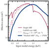 |
Fig. A.1. Comparison of the single ARF (red solid) and the “stacked ARF” (blue solid) extracted from the stacked full response of the spec-z sample. We also demonstrate the way we correct for Galactic absorption for each source, that is, taking an energy-bin-wise product between the single ARF and Galactic absorption profile (red dashed), with the column density fixed at the value corresponding to that source. |
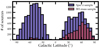 |
Fig. A.2. Galactic latitude distribution of our spec-z and BH-mass sample. We note that ≳90% of sources in both samples have a relatively high Galactic latitude (|l|> 30°), where the Galactic medium is less clumpy and the estimation of column density from NH tool is more reliable. |
Since the PI spectrum and the full response Pij are coupled together through Eq. (A.3), a rest-frame correction must also be applied to Pij, to match the PI shifting. The Pij matrix is nearly diagonal and two-dimensional, with rows corresponding to input model energy bins and columns to output detector channel energies. Each row sums to the effective area at the respective input energy, as encoded in the ARF’s SPECRESP extension. The rest-frame correction of Pij involves two steps:
-
Horizontal shift (along output channel energy axis): For each row, we shift the grids horizontally by 1 + z while keeping the column bin edges fixed. When the shifted grid spans more than one channels (column bins), we allocate the grid value in each channel proportional to the overlapping width, following the same procedure as PI shifting. This step automatically broadens the energy dispersion (inverse of spectral resolution) by 1 + z.
-
Vertical shift (along input model energy axis): Then for each column, we shift the grids vertically by 1 + z, while keeping the row bin edges fixed. If a row bin overlaps with multiple shifted grids, a weighted average is computed based on the overlap width between the shifted grid and the row bin.
A.3. Spectral stacking
To reach as high a signal-to-noise ratio as possible while preserving Poisson statistics, we summed the rest-frame PI spectra of all sources (indexed by l) directly:
 (A.4)
(A.4)
The uncertainty of an energy bin with spectral counts N follows a Poisson distribution. Unlike the routine of optical spectral stacking, we do not scale the spectra to a common flux level, which would deviate from Poisson statistic and pose additional challenges when estimating the uncertainty.
Because the sum of Poisson processes with expectation λil is a Poisson process with the expectation ∑lλil, we could sum up Eq. (A.3) for all sources, and rewrite it as
 (A.5)
(A.5)
where
 (A.6)
(A.6)
 (A.7)
(A.7)
Here we have assumed that the responses have been mapped onto a common rest-frame energy grid. We have not made the assumption ∑lRijl × Ajl = ∑l(Rijl) × ∑l(Ajl), i.e., that the ARFs and RMFs can be stacked separately, as made in other spectral stacking tools.
We first treat the second term BKG, i.e., the background contribution. A first-order approximation of bil is Bil × Rbkgl, where Bil is the background counts of the lth source, and Rbkgl is the corresponding source-to-background ratio, calculated via  . Here t is exposure time, b is BACKSCAL parameter (the expected size of internal background), a is AREASCAL parameter (the effective area scaling factor); B for background extraction region, and D for source extraction region12.
However, it is important to consider that Rbkg varies from source to source, meaning that ∑lBil × Rbkgl does not follow a Poisson process, and therefore we cannot simply estimate the background uncertainty as  . Thus, we adopted a different and robust method that nevertheless allowed us to estimate the background uncertainty. We first divide the whole sample into ten groups of similar Rbkg. For each group, the background counts are summed, and the uncertainty is calculated assuming approximate Poisson statistics, with the error scaling as
  . Since the photon counts in each channel are sufficiently large now (valid for Gaussian approximation, Poisson(λ)≈𝒩(λ, λ)), we stack the 10 background spectra, scaling with the average source-to-background ratio (
 ) in each group, and calculate uncertainty in each channel with standard Gaussian error propagation. In summary, we approximated the background contribution as
 (A.8)
(A.8)
We note that we nevertheless estimated the expectation of background as ∑lBil × Rbkgl, which is slightly more accurate than grouping into k groups, given that Rbkg has some scatter even in the same group.
We then treat the first term of Eq. (A.7), MODEL, i.e., the source model contribution. The minimum assumption of spectral stacking is that all sources to be stacked share the same spectral shape, and therefore we can rewrite Fjl as  , where
  is the normalization of source l that does not vary across index j (the input model energy). With that in mind, we further transform the first term of Eq. (A.7) into
 (A.9)
(A.9)
 (A.10)
 (A.11)
 (A.12)
with the response weighting factor, Wl, being
 (A.13)
In practice, we estimated Wl in a pure data-driven way based on Eq. (A.3):
 (A.14)
Ideally if the spectral counts is large enough and all sources really share the same spectral shape,  should be nearly identical across the entire output channel energies (i). This is of course not the case in reality, and we therefore integrate over a broad energy range (rest-frame 1.0 − 2.3 keV) to obtain an average value. The choice of 1.0 − 2.3 keV is optimal for eROSITA, as it includes sufficient photon counts while deliberately exclude energies below 1 keV to minimize contamination by absorption. We assume a Γ = 2 power law with normalization of 1 for
  . Choosing a different spectral shape (e.g., a power law with Γ = 0) changes the ultimate stacked response by ≲1% and therefore does not affect our results. As we are only interested in the shape of the stacked spectrum, we choose the
  normalization arbitrarily, and further normalize Wl to Wnorml = Wl/∑lWl. The final stacked full response, to be inserted back to Eq. (A.12), is calculated as
 (A.15)
We note the similarity between Eq. (A.12) and the first term of Eq. (A.3). This is to say, with the stacked PI spectrum, stacked background PI spectrum, and stacked response, we can proceed with spectral fitting just as we often do for the single source, to infer the real average model  . Due to the Gaussian nature of the background, the PG-statistic (pgstat) is used.
A.4. Implementation of code and notes
The complete spectral stacking procedure is implemented in our publicly available code, Xstack (https://github.com/AstroChensj/Xstack/). To summarize, we stack the individual PI spectra as Eq. (A.4), stack the individual background spectra and estimate uncertainty with Eq. (A.8), and take the weighted sum of the full response following Eqs. (A.14) and (A.15). All individual spectra and responses have already been shifted on the same rest-frame energy grid (Appendix A.2). The resulting stacked PI spectra, background PI spectra, and full responses (from which we can extract ARF and RMF) are fully prepared for spectral fitting. While the normalization of the stacked spectra is not physically meaningful due to the nature of our stack, our method robustly preserves spectral shapes, enabling reliable analysis of spectral trends and parameter dependences.
Below we make some additional comments:
-
The response weighting factor Wnorml essentially characterizes the relative contribution of each source to the stacked spectrum. In Fig. A.3 we present the histogram of Wnorml for the BH-mass and spec-z sample (see Section 2.1 for definition of the two samples). The extremely high count sources (orange histogram) are also at the high end of the Wnorml distribution, but have some dispersion due to the redshift distribution. The majority of sources sit around the median values, and no significant outliers are seen.
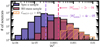
Fig. A.3. Distribution of normalized response weighting factor. As in Fig. 1, the spec-z sample (purple filled), the BH-mass (red filled), and over-bright sources in spec-z sample (orange hatched) are shown, as well as median values with vertical dashed lines. The weighting factors, a combination of source counts and effective area in the 1.0 − 2.3 keV range, are distributed over several orders of magnitude.
-
By taking the inter-source flux variation into account, our data-driven response weighting method can characterize the mean sample spectrum with less bias than for example by exposure. Different approaches are tested with simulations in Appendix B.1.
-
From the stacked full response we can extract an “effective” ARF and RMF. The ARF can be derived by summing Pijstack along the output channel energy axis, while dividing Pijstack by the ARF yields the RMF. We plot the effective stacked ARF and RMF in Fig. A.1 (blue solid line) and Fig. A.4 (middle panel and blue curve in the right panel) respectively, in comparison with the ARF and RMF for a singlesource. The shape of the stacked ARF is clearly different from that of a single ARF. For the stacked RMF, we can also see two major differences from the single RMF: 1) the off-axis features, prominent in the single RMF, are now blurred and smoothed in the stacked RMF; 2) the diagonal of the stacked RMF becomes thicker than that in the single RMF. Indeed, by fitting each row (input model energy) of the RMF matrix with a Gaussian, the right panel of Fig. A.4 shows how the spectral energy dispersion (characterized by FWHM) in the stacked RMF are systematically larger than those in the single RMF. This apparent degradation of the spectral resolution mainly stems from the response shifting process (rather than the stacking process), where the rest-frame energy dispersion FWHMrest at Ej is actually 1 + z times the observer-frame energy dispersion FWHMobs at Ej/(1 + z), and from the relation between dispersion and energy for a single RMF (red curve in right panel of Fig. A.4) it can be read that FWHMEj/(1 + z)obs > FWHMEjobs/(1 + z). Therefore, FWHMEjrest = (1 + z)⋅FWHMEj/(1 + z)obs > FWHMEjobs.
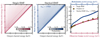
Fig. A.4. Effect of stacking RMFs. Left panel: Observer-frame eROSITA RMF of a single source. Here the color indicates the probability. Weak off-diagonals are visible. Middle panel: Rest-frame “stacked RMF” extracted from the stacked full response of the spec-z sample. Off-diagonals are less prominent, while the width of the diagonal becomes larger compared with a single RMF. Right panel: Spectral energy dispersion (FWHM of the RMF matrix diagonal) at different input model energies (observer-frame for the single RMF, while rest-frame for the stacked RMF) quantifying the spectral resolution. The energy dispersion increases with energy (resolution decreases with energy). The observer-frame energy dispersion of a single source (red curve) is lower than the rest-frame energy dispersion of the spec-z sample (blue). The standard measurement of eROSITA energy resolution from Table 4 of Predehl et al. 2021 (7 TMs averaged) is also listed as orange diamonds.
Appendix B: Robustness checks
In this section, we test the robustness of our results. We first perform a single power law simulation to validate our X-ray spectral stacking procedure in Appendix B.1. We check whether our choice of K-correction slope would result our results in Appendix B.2. We also check whether several sample selection bias would affect our conclusions in Appendix B.3. Finally, we compare the brightest 5 sources with the stacked spectra in each of the 3 × 3 MBH − λEdd bin, as a sanity check for our optical-UV X-ray stacking.
B.1. Simulation to validate stacking
To validate our stacking procedure, we perform simulation using XSPEC command fakeit. For simplicity, we adopt a power law absorbed by the Galactic medium, TBabs*zpowerlw, as the input model. The photon index is assumed to follow a Gaussian distribution with a mean of 2 and a standard deviation of 0.2. The redshift, Galactic absorption column density, 0.3 − 2.3 keV observer-frame flux, exposure time, background and ARF, are based on real sources, sampled from 500 random sources in our dataset. These parameters ensure that the simulated Galactic-absorbed power laws share similar spectral qualities to the real sample. The median of input spectral shape (before being absorbed by Galactic medium) is plotted in Fig. B.1 as gray horizontal (Γ = 2) solid line. We then apply three different methods to stack them, and present the stacked spectra in Fig. B.1. Common to the three methods, we sum the rest-frame PI counts directly. For the yellow points (labeled “CTS/RSP”) we apply our data-driven response weighting method (Eq. (A.14)) and Galactic-absorption correction, whereas for the green points (labeled “CTS/RSP, GalNH-uncorr”) we use the same response weight, but do not apply Galactic absorption correction. For the red points (labeled “EXPO”), we weigh each response by exposure time.
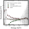 |
Fig. B.1. Simulation results. For a family of mock power laws with varying photon indices (centered at 2), redshift, Galactic absorption, exposure time, background, and response (all taken from real values), Xstack produces the stacked spectrum (assuming our data-driven response weighting factors) as yellow dots (“CTS/RSP”), resembling the input median power law well. For comparison, we present the stacked spectrum without Galactic absorption correction (green dots, “CTS/RSP,GalNH-uncorr”), and the stacked spectrum taking exposure as response weighting factors (red dots, “EXPO”). They both reproduce much more biased spectral shapes. |
The stacked spectrum generated using our data-driven response weights (yellow curve, Γ ∼ 1.96) closely aligns with the input median (gray horizontal line, Γ = 2), highlighting the reliability of our stacking method. Below 0.3 keV, we observe minor artifacts that likely originate from low source completeness in this energy range. And this is also the reason why we have discarded below 0.3 keV in the scientific analysis (Section 3.2).
In the meantime, we see that the two other methods all produce significantly biased spectral shape compared to input, especially towards the soft end. Weighting response by exposure time is a rather simplified method, and would only be identical to our data-driven method when all sources have the same flux in the 1.0 − 2.3 keV band. As can be seen, while this approach reproduces the hard X-ray part reasonably well, it produces a large artifactual excess in the soft band, resulting in an overall softer (Γ ∼ 2.12) spectrum than expected (Γ = 2). This emphasizes the importance of accounting for inter-source flux variation during stacking. On the other side, from the green points we see that the Galactic absorption significantly suppress the stacked spectrum up to ∼3 keV, thus highlighting the need to correct for it during the stacking.
B.2. Validity of constant SED slope for UV K-correction
To derive the rest-frame UV luminosity of each source, we apply a K-correction assuming a constant UV SED slope of α = −0.65. However, as shown by Hagen et al. 2024b and also our Fig. 8, the UV slope actually evolves with λEdd (and slightly with MBH). Ideally, one could iteratively stack the UV SED within bins of MBH and λEdd, updating the assumed SED slope for K-correction at each step, until convergence to an “optimal” value is achieved. This would, however, require λEdd, MBH, and g, u photometry from SDSS, which is not applicable to all sources in our sample (especially the “spec-z” sample). We therefore simply adopt a uniform constant slope for the K-correction across all sources, regardless of their physical properties. Below, we perform simple tests to validate that our conclusions are robust against this choice.
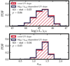 |
Fig. B.2. Upper panel: Comparison between the UV luminosity derived with K-correction assuming a constant UV SED slope α = −0.65, and that assuming a MBH-λEdd-dependent slope. The KS test statistics as well as p-values are also listed. We generally do not see significant differences between the two distributions. Lower panel: Same as upper panel but comparing αox instead. |
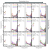 |
Fig. B.3. Same as Fig. 8 but also showing the individual spectra of the brightest five sources in each MBH – λEdd bin as colored curves. These generally show the same trends as the stacked re-binned data (yellow dots with error bars) and unbinned data (gray error bars). |
We select a representative subsample from our “BH-mass” and “spec-z” sample, consisting of sources located within the 3 × 3 grid in Fig. 2. Since we have stacked UV spectra for this subsample (Fig. 8), we can use them to update our knowledge of the MBH-λEdd-dependent UV SED slopes. (For simplicity, we do not perform further iterations to refine the slopes.) Using these updated slopes, we recalculate the K-corrected UV luminosity log(νLν)UV and αox for each source, and compare them to the values obtained under the assumption of a constant slope α = −0.65. The comparisons are shown in Fig. B.2, along with KS test statistics and p-values. From the upper panel we see that the distribution of log(νLν)UV remains nearly unchanged even after applying the updated slopes, with only marginal differences (p = 0.06). A similar conclusion holds for αox, as shown in the lower panel. Therefore our conclusions in Sections. 5.2 and 5.3 are not affected.
Finally, we examine whether our conclusions based on AGNSED fit (Section 6) are affected by applying the updated, MBH-λEdd-dependent UV slopes for K-correction. We find that the changes in the best-fit AGNSED parameters (notably, the warm corona radius RWC) are all within 1σ uncertainties. This is in fact understandable, as for our UV stacking pipeline (Fig. 8), we have already assigned additional uncertainties to the stacked UV SED to account for potential systematics, including the uncertainties in K-correction slope.
B.3. Robustness against sample selection bias
We also check the robustness of our conclusions against potential sample selection bias. We first account for the NUV non-detected sources in each of the 3 × 3 grid in Fig. 8, that is, we select all SDSS-eROSITA sources within the GALEX field of view, regardless of NUV detected or not. In stacking optical-UV X-ray SED, these NUV non-detected sources contribute eROSITA X-ray, SDSS g and u data, but no GALEX NUV flux, leading to a downward trend in the UV. After fitting the resulting SED with the same procedure as Section 4.2, we find very small changes in all AGNSED parameters, which is expected as the overall NUV completeness in our BH-mass sample is as high as ∼93% (Section 2.1). Secondly, we check if our conclusions still hold for a lower redshift subsample. Although the majority of sources in our BH-mass sample have relatively low redshift (z < 1), there is still a portion with high redshift (z > 1), reaching the EUV regime and thereby bringing in more IGM absorption, potentially biasing the entire SED. Focusing on a subsample of z < 1 and doing the spectral fitting again on the 3 × 3 grid, we find that correlations between warm-hot corona radius and λEdd and MBH are still preserved.
B.4. Brightest five sources in each 3 × 3 grid
We compare the spectra of the brightest 5 sources to the stacked SED in each of the 3 × 3 grid in Fig. B.3. The individual sources are shifted to rest-frame, in the same way as the stacked spectra illustrated in Appendix A.2 (X-ray) and Section 4.1 (UV). Since the individual spectra have rather poor spectral quality at 4 keV, we normalize them at ∼2 keV to the same flux of the normalized stacked spectrum. Although these bright sources still have very limited photon counts (∼200 within 0.2 − 10.0 keV) for reliable spectral modeling, it is noticeable that these individual sources generally follow the same trend as those observed in the stacked spectra. In particular, the soft excess becomes stronger for increasing λEdd and decreasing MBH, and the UV to X-ray ratio becomes stronger for increasing λEdd but does not correlate well with MBH.
Appendix C: Star formation contamination in low λEdd – high MBH bins
In Fig. C.1 we present the estimated NUV flux (in μJy) of galaxies on the star formation main sequence (SFMS), shown as black and gray points. These points are derived from an ensemble of GRAHSP (Buchner et al. 2024) models, selected with star formation rate SFR< 300 M⊙.yr−1, specific star formation rate −10.5< logsSFR< − 9.5, and dust attenuation E(B-V)< 0.03 to approximate the SFMS. Additionally, an AGN luminosity cut logLAGN< 40 is applied to exclude AGN contributions.
Assuming stellar-to-SMBH mass ratio of ∼200, we plot in the left panel the predictions for high mass galaxies (log M* > 10.5) from GRAHSP, alongside corresponding quasars (AGN+host) with log MBH > 8.5 from our sample. We find that the NUV flux from SFMS massive galaxies can reach up to 200 μJy, which is similar to the low λEdd quasars (red) in our sample, and only slightly below the medium (green) and high (blue) λEdd quasars. On the contrary, the right panel shows the fluxes from low mass SFMS galaxies (log M* < 10.5) and corresponding quasars with log MBH < 8.5 from our sample (yellow, with no further differentiation by λEdd). Here, the fluxes from SFMS galaxies are consistently smaller than those from the quasars. These suggest that the real AGN contributions in the low λEdd – high MBH could be significantly smaller, if their host galaxies really lie on SFMS.
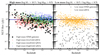 |
Fig. C.1. Estimated NUV flux of SFMS galaxies with high mass (black points in the left) and low mass (gray points in the right), and the observed NUV flux of quasars in our sample with high mass (red for low λEdd, green for medium λEdd, blue for high λEdd) and low mass (yellow). |
All Tables
Spectral fitting results for the phenomenological model of different αox, LUV, λEdd or MBH binnings.
All Figures
|
Fig. 1. Distribution of 1.0 − 2.3 keV net counts (top panel), spectroscopic redshifts (middle panel), and 2 keV monochromatic luminosity LX (bottom panel) for our spec-z (purple filled), BH-mass (red filled), and over-bright sources in the spec-z sample (orange hatched), respectively. The median value for spec-z (BH-mass) sample is marked with purple dashed (red dashed) lines. |
| In the text | |
|
Fig. 2. Distribution of MBH and λEdd of our BH-mass sample, with color mapping density. The 3 × 3 MBH-λEdd grid is shown as blue transparent boxes. |
| In the text | |
|
Fig. 3. Summed eROSITA spectrum from 23 Ms of observations (“spec-z” sample). To reveal the intrinsic spectral shape of AGN, the spectrum is divided by the ARF and multiplied by E2 (so the unit proportional to keV2 Counts cm−2 s−1 keV−1 or erg cm−2 s−1), normalized at 4 keV. The gray points are the unbinned data, while yellow circles show a logarithmic rebinning. The yellow shaded area, derived from bootstrapping the sample for 100 times, indicates the 68% uncertainty range of the spectrum from both stacking process and Poisson fluctuation (the plotting routine also applies to Figs. 4–8). Only the spectrum between 0.3 keV and 8 keV is used in this work. Between 1 and 6 keV, the spectrum is approximately linear in this log-log plot, while below, the spectrum bends upwards. Between 6 and 7 keV, a bump is visible despite the relatively larger errorbars. Power laws of typical photon indices are plotted only for visual comparison. |
| In the text | |
|
Fig. 4. Stacked spectra in three equally sized groups (colored lines) divided by αox, LUV, λEdd, and MBH (panels from left to right). The legend gives the mean value of each subgroup. Error bars are obtained with bootstrapping as in Fig. 3, but are generally very small except above ∼8 keV. In the left panel, the three colored lines are indistinguishable above 2 keV. Below 1 keV, the blue data points from the lowest αox subsample are always below the pink points from the highest αox subsample. The λEdd panel shows an even larger spread between subgroups, while it is less pronounced in the LUV panel and reversed in the MBH panel. |
| In the text | |
|
Fig. 5. Difference spectrum between the highest and lowest αox subgroups from the left panel of Fig. 4 highlighting the spectral shape of the emerging soft excess component. The binned yellow data follow a line in this log-log plot corresponding to a Γ = 3.2 power law (dashed purple line), but fall below beyond 1 keV. The horizontal lines mark where the flux (E2N) of the difference spectrum amounts to 100%, or 10% of the original normalized spectra at 4 keV, where the spectra are normalized. The yellow data points are above the 1x line below 0.5 keV, and below the 0.1x line above 2 keV. Above 3 keV, the difference falls below 1%. |
| In the text | |
|
Fig. 6. Fits to stacked spectra (from “spec-z” sample) in equally sized bins of αox (top panels) and LUV (bottom panels). The legend gives the mean value of each subgroup, the number of stacked sources, and the fitting statistics. The soft power law (green) and the hard power law (blue) as well as the sum (black) are shown. Each curve is the best fit to a bootstrap realization of the sample. In the top panels, from the left to right panels, the green curves move upwards. The strengthening of the soft excess is quantified by q with error bars, increasing from 0.13 to 0.58. The bottom panels show fewer changes in the green warm corona component with LUV. |
| In the text | |
|
Fig. 7. Similar to Fig. 6 but for λEdd (top panels) and MBH (bottom panels) using the “BH-mass” sample. In the top panels, from the left to right panels, the green soft excess component curves move upwards, and the soft excess strength, q, increases from 0.13 to 0.52. |
| In the text | |
|
Fig. 8. Optical-UV X-ray SED on our 3 × 3 MBH-λEdd grid overlaid by best-fit bootstrap models, with red for disk (DK), green for warm corona (WC), and blue for hot corona (HC). The legend gives the source number, median MBH, λBH, best fitting statistic in each bin. A toy model illustrating the disk-corona size (warm corona radius RWC, hot corona radius RHC, both in units of Rg) is shown on the top right of each panel. We note the potential star-formation contamination in two upper-left bins with low λEdd – high MBH when interpreting the results. |
| In the text | |
|
Fig. 9. Best-fit AGNSED models for our 3 × 3 MBH-λEdd grids (excluding the two with potential star formation contamination). Different components are shown with the same color convention as in Fig. 8. As no data are involved, we scaled the y-axis to physical values (erg s−1) by setting the AGNSED distance parameter as dL = 100 Mpc and the normalization to 4πdL2. |
| In the text | |
|
Fig. 10. Evolutionary trend of the hot corona radius RHC (left), warm corona radius RWC (middle), and warm corona “size” log(RWC2 − RHC2) (right) on the 3 × 3 MBH-λEdd grid. The color is linearly interpolated for visualizing trends. The two low λEdd – high MBH bins are grayed out for star-forming contamination (see text for details), except for which the warm corona radius shows a clear increasing trend with increasing λEdd and decreasing MBH. The hot corona radius decreases with increasing λEdd while remains constant for different MBH. |
| In the text | |
|
Fig. 11. Sketch summarizing the physical picture of disk-to-warm corona transition. A hydrogen ionization instability at ∼1 × 10⁴ K within the disk likely triggers the formation of the warm corona. For either a more massive BH or a lower Eddington ratio, the disk temperature becomes cooler, causing the transition radius (in terms of Rg) to move inward. Meanwhile, the hot corona expands (in units of Rg) as Eddington ratio decreases, to match the observed increase in Xray-to-bolometric luminosity fraction. |
| In the text | |
|
Fig. 12. B-band (κbol, o, orange) and hard X-ray (κbol, 2 − 10, blue) bolometric correction factors for our stacked optical-UV X-ray SEDs, as a function of “refined” bolometric luminosity (top panel), “refined” Eddington ratio λEdd* (middle panel), and BH-mass MBH (bottom panel). Points with a similar Eddington ratio (λEdd, taken from Wu & Shen 2022) are connected with lines and share the same color. The points overall straddle the literature relations from Duras et al. 2020. |
| In the text | |
|
Fig. A.1. Comparison of the single ARF (red solid) and the “stacked ARF” (blue solid) extracted from the stacked full response of the spec-z sample. We also demonstrate the way we correct for Galactic absorption for each source, that is, taking an energy-bin-wise product between the single ARF and Galactic absorption profile (red dashed), with the column density fixed at the value corresponding to that source. |
| In the text | |
|
Fig. A.2. Galactic latitude distribution of our spec-z and BH-mass sample. We note that ≳90% of sources in both samples have a relatively high Galactic latitude (|l|> 30°), where the Galactic medium is less clumpy and the estimation of column density from NH tool is more reliable. |
| In the text | |
|
Fig. A.3. Distribution of normalized response weighting factor. As in Fig. 1, the spec-z sample (purple filled), the BH-mass (red filled), and over-bright sources in spec-z sample (orange hatched) are shown, as well as median values with vertical dashed lines. The weighting factors, a combination of source counts and effective area in the 1.0 − 2.3 keV range, are distributed over several orders of magnitude. |
| In the text | |
|
Fig. A.4. Effect of stacking RMFs. Left panel: Observer-frame eROSITA RMF of a single source. Here the color indicates the probability. Weak off-diagonals are visible. Middle panel: Rest-frame “stacked RMF” extracted from the stacked full response of the spec-z sample. Off-diagonals are less prominent, while the width of the diagonal becomes larger compared with a single RMF. Right panel: Spectral energy dispersion (FWHM of the RMF matrix diagonal) at different input model energies (observer-frame for the single RMF, while rest-frame for the stacked RMF) quantifying the spectral resolution. The energy dispersion increases with energy (resolution decreases with energy). The observer-frame energy dispersion of a single source (red curve) is lower than the rest-frame energy dispersion of the spec-z sample (blue). The standard measurement of eROSITA energy resolution from Table 4 of Predehl et al. 2021 (7 TMs averaged) is also listed as orange diamonds. |
| In the text | |
|
Fig. B.1. Simulation results. For a family of mock power laws with varying photon indices (centered at 2), redshift, Galactic absorption, exposure time, background, and response (all taken from real values), Xstack produces the stacked spectrum (assuming our data-driven response weighting factors) as yellow dots (“CTS/RSP”), resembling the input median power law well. For comparison, we present the stacked spectrum without Galactic absorption correction (green dots, “CTS/RSP,GalNH-uncorr”), and the stacked spectrum taking exposure as response weighting factors (red dots, “EXPO”). They both reproduce much more biased spectral shapes. |
| In the text | |
|
Fig. B.2. Upper panel: Comparison between the UV luminosity derived with K-correction assuming a constant UV SED slope α = −0.65, and that assuming a MBH-λEdd-dependent slope. The KS test statistics as well as p-values are also listed. We generally do not see significant differences between the two distributions. Lower panel: Same as upper panel but comparing αox instead. |
| In the text | |
|
Fig. B.3. Same as Fig. 8 but also showing the individual spectra of the brightest five sources in each MBH – λEdd bin as colored curves. These generally show the same trends as the stacked re-binned data (yellow dots with error bars) and unbinned data (gray error bars). |
| In the text | |
|
Fig. C.1. Estimated NUV flux of SFMS galaxies with high mass (black points in the left) and low mass (gray points in the right), and the observed NUV flux of quasars in our sample with high mass (red for low λEdd, green for medium λEdd, blue for high λEdd) and low mass (yellow). |
| In the text | |
Current usage metrics show cumulative count of Article Views (full-text article views including HTML views, PDF and ePub downloads, according to the available data) and Abstracts Views on Vision4Press platform.
Data correspond to usage on the plateform after 2015. The current usage metrics is available 48-96 hours after online publication and is updated daily on week days.
Initial download of the metrics may take a while.