| Issue |
A&A
Volume 701, September 2025
|
|
|---|---|---|
| Article Number | A236 | |
| Number of page(s) | 22 | |
| Section | Numerical methods and codes | |
| DOI | https://doi.org/10.1051/0004-6361/202554951 | |
| Published online | 23 September 2025 | |
Efficient simulation of discrete galaxy populations and associated radiation fields over the first billion years
1
Scuola Normale Superiore di Pisa,
Piazza dei Cavallieri 7,
56126
Pisa,
Italy
2
Centro Nazionale “High Performance Computing, Big Data and Quantum Computing”,
Italy
★ Corresponding author: This email address is being protected from spambots. You need JavaScript enabled to view it.
Received:
1
April
2025
Accepted:
23
July
2025
Abstract
Understanding the epochs of cosmic dawn and reionisation requires us to leverage multi-wavelength and multi-tracer observations, with each dataset providing a complementary piece of the puzzle. To interpret these data, we updated the public simulation code, 21cmFASTv4, to include a discrete source model based on stochastic sampling of conditional mass functions and semi-empirical galaxy relations. We demonstrate that our new galaxy model, which parametrises the means and scatters of well-established scaling relations, is flexible enough to characterise a range of predictions from different hydrodynamic cosmological simulations of high-redshift galaxies. Combining a discrete galaxy population with approximate, efficient radiative transfer allows us to self-consistently forward-model galaxy surveys, line intensity maps (LIMs), and observations of the intergalactic medium (IGM). Not only does each observable probe different scales and physical processes, but their cross-correlation will maximise the information gained from each measurement by probing the galaxy-IGM connection at high redshift. In this work, we found that a stochastic source field produces significant shot-noise in 21cm and LIM power spectra. Scatter in galaxy properties can be constrained using ultraviolet (UV) luminosity functions and/or 21cm power spectra, especially if astrophysical scatter is higher than expected (as might be needed to explain recent JWST observations). Our modelling pipeline is both flexible and computationally efficient, thereby facilitating high-dimensional, multi-tracer, field-level Bayesian inference of cosmology and astrophysics over the first billion years.
Key words: galaxies: high-redshift / intergalactic medium / dark ages, reionization, first stars
© The Authors 2025
 Open Access article, published by EDP Sciences, under the terms of the Creative Commons Attribution License (https://creativecommons.org/licenses/by/4.0), which permits unrestricted use, distribution, and reproduction in any medium, provided the original work is properly cited.
This article is published in open access under the Subscribe to Open model. This email address is being protected from spambots. You need JavaScript enabled to view it. to support open access publication.
1 Introduction
The epoch of reionisation (EoR) and cosmic dawn (CD) mark the formation of the first galaxies, whose multi-wavelength radiation heated and ionised the pervasive intergalactic medium (IGM). The history and morphology of this IGM phase transition encode a wealth of information about cosmology, large-scale structure formation, and the astrophysics of the first galaxies.
Current and upcoming observations of the EoR and CD come from a wide variety of sources. The brightest few galaxies are being seen individually by optical and infrared (IR) telescopes, such as the Hubble space telescope1, the James Webb Space Telescope (JWST)2, the Very Large Telescope (VLT)3, and in the future by the Nancy Grace Roman space telescope4 and the Extremely Large Telescope (ELT)5. Line intensity mapping (LIM) experiments such as the ATacama Large Aperture Submilimetre Telescope (AtLAST)6 and the Fred Young Sub-milimetre Telescope (FYST)7, and the Spectro-Photometer for the History of the Universe, Epoch of Reionization and Ices Explorer (SPHEREx)8 will observe the large-scale, integrated flux of all galaxies, using transitions in the interstellar medium (ISM) such as CO, CII and Lyman alpha (e.g. see the review in Bernal & Kovetz 2022). The Lyman alpha forest in the spectra of high-z QSOs already gives strong constraints on IGM properties at z < 6 (e.g. D’Odorico et al. 2023; Qin et al. 2025). Arguably the most revolutionary probe will come from the spin-flip transition of HI. This 21cm line will allow us to eventually map the IGM during the first billion years, resulting in a cosmological dataset of unprecedented size and quality (e.g. see the review in Mesinger 2019).
These multi-tracer observations are highly complementary. Combining them in a self-consistent analysis framework is fundamental for extracting the maximum cosmological and astrophysical information. This is especially true with preliminary, low signal-to-noise (S/N) EoR/CD datasets, which must be combined in order to meaningfully constrain theoretical models (e.g. see Figure 8 and associated discussion in Breitman et al. 2024). Analysing diverse datasets will also allow us to identify possible tensions between observations, which can act as signposts for new physics and/or systematics.
Unfortunately, it is not easy to construct a self-consistent, flexible modelling framework for multi-tracer EoR/CD observations. Galaxy formation is a highly non-linear processes, with cosmic radiation fields coupling a vast range of scales. Furthermore, the unknown physics of early galaxy formation means that models calibrated to low-redshift data can give very different predictions at high redshifts and/or small masses where current data is lacking (e.g Ni et al. 2023; Lovell et al. 2024). As a result, theoretical modelling pipelines of EoR/CD datasets need to be accurate, flexible, and fast enough to explore the large parameter space of uncertainties.
These requirements have motivated development of so-called semi-numerical simulations (e.g. Mesinger & Furlanetto 2007; Visbal et al. 2012; Mutch et al. 2016; Croton et al. 2016; Choudhury & Paranjape 2018; Hutter et al. 2021). Semi-numerical simulations make trade-offs between accuracy and speed, so that they can be used in data-driven analyses from a combination of IGM and galaxy observations (e.g. Greig & Mesinger 2015; Choudhury et al. 2021; Qin et al. 2021a; Abdurashidova et al. 2022; Nikolic´ et al. 2023; Mutch et al. 2024). Starting from large-scale, 3D realisations of initial conditions, linear and quasi-linear evolution is often performed using higher-order perturbation theory (e.g. Scoccimarro 1998) to avoid costly N-body simulations, while non-linear structure formation may be captured with an excursion-set approach (e.g. Mesinger & Furlanetto 2007). Galaxy properties can be parametrised with a choice of physical or empirical functional forms. The corresponding emissivities are used to perform multi-band cosmological radiative transfer using approximations that are reasonably accurate on moderate to large scales (≳ cMpc; e.g. Mesinger et al. 2011; Zahn et al. 2011; Ghara et al. 2018; Hutter 2018). As a result, semi-numerical simulations can generate 3D lightcones of various IGM properties in roughly 1 core hour: many orders of magnitude faster than more detailed cosmological radiative transfer simulations.
However, some approximations that are currently made in semi-numerical simulations could limit their usefulness when interpreting certain observations. For example, a common assumption is that each ~cMpc simulation cell contains the average conditional halo mass function and corresponding galaxy emissivity, given its density, velocity, temperature, and ionisation state. This is typically justified by the fact that radiation fields and associated IGM properties are determined by the combined radiation of many sources. In some cases, however, neglecting galaxy-to-galaxy scatter could bias our interpretation of EoR/CD data (see e.g. Ren et al. 2019; Gelli et al. 2024; Nikolic´ et al. 2024).
Furthermore, some observations might require modeling individual galaxies and their surrounding EoR morphology (e.g. Lu et al. 2025; Nikolic´ et al. 2025). Modelling individual galaxies in large-scale simulations currently requires either expensive N -body codes (e.g. Choudhury & Paranjape 2018; Ghara 2023; Schaeffer et al. 2023) or somewhat faster Lagrangian halo finders (e.g. Monaco et al. 2002; Mesinger & Furlanetto 2007); these add significant computational and memory overheads limiting their use in Bayesian inference pipelines.
In this work, we introduce a fast, stochastic source model implemented in the new version of the public code 21cmFASTv49. Using a combination of Lagrangian halo finding and coarse time-step merger trees, we are able to rapidly build 3D realisations of dark matter halos throughout the EoR/CD. These are then populated with galaxies by sampling well-established empirical relations, such as the stellar-to-halo relation (SHMR), the star-forming main sequence (SFMS), and the fundamental mass metallicity relation (FMR). The parameters of these relations (e.g. mean, scatter, temporal correlation) form a flexible, easy-to-interpret astrophysical basis, allowing us to infer them from observations. Now, 21cmFASTv4 is able to explicitly account for stochastic galaxy formation, as well as generate 3D lightcones of galaxy properties (e.g. stellar mass, star formation rate) together with the corresponding IGM lightcones. As illustrated in Figure 1, this allows us to rapidly and self-consistently forward-model galaxy maps, LIMs, and IGM observations, as well as the corresponding cross-correlations.
This paper is organised as follows. Section 2 describes how we sample halo masses in a simulation volume. Section 3 details how galaxy properties such as stellar mass, SFRs, and metallici-ties are assigned to each halo. Section 4 describes the calculation of radiative backgrounds from the new discrete sources and their effect on the IGM. Section 5 presents results from a fiducial simulation, showing how the new source model drives the EoR/CD. Section 6 compares our new source model to previous iterations in 21cmFAST, detailing the effects the stochastic source model has on our lightcones. Finally, Section 7 shows new outputs of the model, which can be used for analysis, using the cross-correlation between the CII and 21cm intensity maps as an example. We then summarise our work and possible next steps in Section 8. Throughout this paper, we use comoving units unless stated otherwise, as well as the following cosmological parameters: {Ωm, Ωb, H0, σ8 = {0.3096, 0.04897, 67.66, 0.8102}.
2 Generating the dark matter halo field
Our goal is to include discrete halos within an inference pipeline that can be sampled rapidly with different initial conditions. N -body codes would be too computationally expensive, given the enormous dynamic range requirements: the first galaxies are hosted by halos with masses of ~106 M⊙, and the volumes required to sample the largest relevant scales during the EoR/CD are ≳(250 Mpc)3 (Iliev et al. 2014; Kaur et al. 2020).
To achieve these requirements, various approximate approaches for populating cells with halos have been explored. The simplest is to integrate over a conditional halo mass function (CHMF) either within cells (Davies & Furlanetto 2022; Trac et al. 2022; Mas-Ribas et al. 2023) or within larger spheres (Mesinger et al. 2011). While these methods are fast, they ignore stochasticity in the halo mass distribution, which could be important for some observables (e.g. Nikolic´ et al. 2024). If we wish to take into account the scatter in the halo mass distribution from the CHMF, we need to generate a population. The first methods for generating these populations rely on the excursion set formalism (Bond et al. 1991), where a random walk is performed on the Lagrangian density field in decreasing smoothing scales, and halos form where this smoothed density crosses a redshift-dependent (and possibly scale dependent) barrier. Such methods require very high resolution density fields to resolve the smallest halos (e.g. Monaco et al. 2002; Mesinger & Furlanetto 2007), which can be very expensive in terms of memory and computational requirements.
Other methods follow binary mergers within a halo mass distribution using small internal time-steps (Cole et al. 2000; Parkinson et al. 2008; Benson et al. 2016; Qiu et al. 2021; Trinca et al. 2022). Such binary merger algorithms can result in halo populations consistent with N -body simulations; however, they require an ‘ad hoc’ calibration to match a target distribution (see Cole et al. (2008) and Appendix B). While it is possible to fit these calibration factors for any particular simulation or mass function, it would be desirable to have a more flexible model that can quickly produce samples from any given CHMF without needing to perform a fit beforehand.
Here, we use a hybrid approach (cf. McQuinn et al. 2007; Nasirudin et al. 2020; Meriot & Semelin 2024) where halos whose masses are comparable or larger than the mass of the Lagrangian cell10 are identified using the existing Lagrangian halo finder of 21cmFAST titled DEXM (Mesinger & Furlanetto 2007). Less massive halos are instead identified with new, coarse-step merger trees that sample conditional halo mass functions (cf. Sheth & Lemson 1999; McQuinn et al. 2007). After this two-stage process, the halos are then moved to Eulerian positions using a second-order Lagrangian perturbation theory (2LPT; e.g. Scoccimarro 1998). We describe the different ingredients of this new method below.
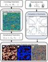 |
Fig. 1 Example usage case for 21cmFASTv4. First, cosmological parameters are sampled, and an associated realisation of the Lagrangian matter field is generated. Dark matter halos are identified in Lagrangian space and then moved, together with the matter field, to Eulerian space using 2LPT. This is shown in the left-middle panel as a slice through a 300 Mpc overdensity field at z = 7, with the 300 largest halos in the 2 Mpc-thick slice shown as red circles. Then galaxies are assigned to DM halos by sampling parametric conditional probability densities based on well-established empirical relations such as the SHMR, SFMS, FMR, etc. Cosmic radiation fields (Lyman-alpha, Lyman-continuum, and X-ray) sourced by these galaxies are calculated using approximate radiative transfer, and the IGM is evolved accordingly. The lower panel shows slices corresponding to the IGM neutral fraction, 21cm brightness temperature, and CII surface brightness density, at the same redshift as the overdensity field and with the same halos overlaid as red circles. We can then extract statistics of these fields for comparison with multi-tracer observations. In the centre-right panel we show the ultraviolet (UV) luminosity function at z = 7, the 21cm power spectrum at the midpoint of reionisation, the evolution of the 21cm power spectrum at k = 0.1 Mpc−1, and the CII x 21cm cross-power spectrum at z = 12. Under fiducial settings, 21cmFASTv4 computes all of these steps in ≲3 core hours for a single realisation, thus facilitating high-dimensional, multi-tracer, field-level Bayesian inference of cosmology and astrophysics during the EoR and CD. |
2.1 Conditional halo mass functions
To distribute halos within a simulation volume more quickly, we use the conditional halo mass function  , which denotes the number density per unit mass of halos of mass, Mh, at a redshift, z, given they reside within a Lagrangian volume of mass, Mcond, and mean overdensity, δcond. The only fully analytic CHMF in widespread use is the extended Press-Schechter (EPS) conditional mass function (Lacey & Cole 1993), which computes the halo mass function from the first time a random walk in decreasing Lagrangian scale, Mh, crosses a critical value of the matter overdensity, δcrit = 1.686/D(z), where D(z) is the linear growth factor. For CHMFs, the origin of the random walk is the value δcond at the scale of Mcond, while the root-mean-square fluctuation of the linear matter field at z = 0, σ(Mh), is set by the assumed cosmology.
The halo mass distribution resulting from this model is
![Mathematical equation: \begin{multline} \frac{dn_\mathrm{EPS}}{dM_h}(M_h,z|\sigma_\mathrm{cond},\delta_\mathrm{cond}) = \frac{\rho_{\mathrm{crit}} \Omega_M}{\sqrt{2\pi} M_h} \frac{2\sigma (\delta_\mathrm{crit} - \delta_\mathrm{cond})}{(\sigma^2 - \sigma_\mathrm{cond}^2)^{3/2}}, \\ \left| \frac{d\sigma}{dM_h} \right| \mathrm{exp} \left[ -\frac{(\delta_\mathrm{crit} - \delta_\mathrm{cond})^2}{2(\sigma^2 - \sigma_\mathrm{cond}^2)} \right], \end{multline}](/articles/aa/full_html/2025/09/aa54951-25/aa54951-25-eq2.png) (1)
(1)
where ρcrit is the critical matter density and we denote σ(Mh) → σ and σ(Mcond) → σcond for brevity. While this model can describe the hierarchical formation of halos over cosmic time, it under-predicts the number of massive halos and over-predicts the number of small mass halos, when compared to N-body simulations (e.g. Tinker et al. 2008). As a result, various methods are applied to correct this function, including altering the shape of the barrier δcrit (Sheth et al. 2001), scaling the CHMF to match total collapsed fraction estimates (Barkana & Loeb 2004; Mesinger et al. 2011), adding corrective terms which scale with δ and σ (Parkinson et al. 2008), or scaling an unconditional mass function by performing variable substitutions similar to the δcrit → (δcrit - δcond) used to compute the EPS CHMF from the unconditional Press-Schechter mass function; Rubiño-Martín et al. 2008; Tramonte et al. 2017; Trapp & Furlanetto 2020.
Here, we use the conditional mass function from Sheth & Tormen (2002), which is approximated using a Taylor expansion of the critical density threshold associated with ellipsoidal collapse, expressed as
 (2)
(2)
with the parameters from Jenkins et al. (2001), namely, a = 0.7, α = 0.81, and β = 0.34. The conditional mass function is then well approximated by
![Mathematical equation: \begin{multline} \frac{dn_\mathrm{ST}}{dM_h}(M_h,z|\sigma_\mathrm{cond},\delta_\mathrm{cond}) = \frac{\rho_{\mathrm{crit}} \Omega_M}{\sqrt{2\pi}M_h} |T(z,\sigma,\sigma_\mathrm{cond})| \\ \frac{d\sigma}{dM_h} \frac{2\sigma}{(\sigma^2 - \sigma_\mathrm{cond}^2)^{3/2}} \mathrm{exp} \left[ \frac{-(B(z,\sigma) - \delta_\mathrm{cond})^2}{2(\sigma^2 - \sigma_\mathrm{cond}^2)} \right], \end{multline}](/articles/aa/full_html/2025/09/aa54951-25/aa54951-25-eq4.png) (3)
(3)
where
 (4)
(4)
While we assume the Sheth–Tormen CHMF for the results shown in this paper, the sampling method implemented in 21cmFASTv4 (and detailed in the remainder of this section) is applicable to any user-defined CHMF.
2.2 Sampling the CHMFs
We build on the 21cmFAST framework by including a fast stochastic source sampler capable remaining self-consistent across cosmic time. We began our sampling at the lowest redshift requested by the user, where each cell in the linearly evolved Lagrangian density grid is used as a condition, determining the CHMF from which we sample using Equation (3). Here, Mcond corresponds to the Lagrangian mass of the cell and δcond is set to the density of our initial conditions field linearly evolved to z = 0. For computational efficiency, we build an interpolation table of the inverse cumulative distribution function of the CHMF and sample it in the mass range [Mmin, Mcell], where Mmin is a free parameter describing our halo mass resolution. We sample the CHMF of each cell Nh times, where Nh itself is drawn from a Poisson distribution11 with a mean of
 (5)
(5)
In Figure 2, we demonstrate the accuracy of this method on the grid scale by showing the mass functions drawn for 10 000 cells of side length 2 Mpc and differing Lagrangian overdensity, compared to the expected conditional mass functions. Both the total number and total mass of halos above the minimum mass can vary significantly between samples.
Since the mass of the Lagrangian cell is determined entirely by the cell size which is uniform throughout the simulation, it is impossible to sample halos with a higher mass from its CHMF. We have used a cell length of 2 Mpc throughout this work, which includes halos up to a mass of 3.11 × 10¹¹ M⊙. To find halos above the cell mass, we utilise the existing halo finder DexM (Mesinger & Furlanetto 2007). DexM works by filtering the initial condition density grid on a series of decreasing scales, identifying halos by the scale at which the Lagrangian density crosses a certain barrier and accounting for mass conservation. In order not to double-count halos that are part of larger structures identified by DexM, we multiply N¯h in each cell by one minus the fraction of mass taken up by these larger halos before sampling the CHMF. Using DexM only once per simulation (as opposed to every redshift) and with the sole aim of finding the largest halos allows us to sample the full halo mass range within our box, while retaining the computational efficiency gained by using the sampler on smaller scales.
If we were to simply repeat this process at each redshift, each halo population would follow the CHMF of the Lagrangian cell in which it resides and would contain the correct mean number and total mass of halos. However, samples in adjacent snapshots would not be correlated with one another; as a result, the halo population in a given region would fluctuate wildly over short periods of time. Since we aim to build lightcones of our halo populations and the resulting radiation fields, we need to correlate the halos sampled at each redshift. To do this, we take our first sample from the lowest redshift as described above, then step back from the descendant redshift, zdesc, to a progenitor redshift, zprog (where zdesc < zprog). We treat each halo as an independent Lagrangian volume and sample from its CHMF setting the condition mass to the descendant halo mass as Mcond = Mdesc and setting the condition density to the SMT barrier at the descendant redshift δcond = B (zdesc, σcond)12 in Equation (3). In the excursion set framework, this is analogous to starting the random walk where the descendant halo crosses the barrier B (zdesc, σcond) at the mass scale, Mdesc, and sampling the mass, M, where paths from this point first cross the higher barrier, B (zprog, σ).
Due to the short time-step and smaller condition masses, the Poisson distribution is no longer a good approximation for the number of halos obtained from a descendant, which tends to be much more narrowly distributed around unity. The use of the Poisson distribution to find progenitors would cause halos to disappear entirely or double in mass on very short timescales. Therefore, instead of limiting the sample by number, we limit it by mass according to the expected mass Mlim of progenitors above our minimum halo mass, Mmin, found by integrating the CHMF as
 (6)
(6)
This effectively assumes that in each descendant halo, a mass of Mcond - Mlim resides in objects below our mass resolution (i.e. obtained by smooth accretion), which are ignored in further sampling.
Once this mass limit is exceeded, the final halo is included if it brings the total mass closer to our target mass, Mlim, allowing for some variance in the total progenitor mass while favouring samples that are closest to the total mass expected13. This process is repeated in successive backward time-steps of zprog = (1 + zdesc)∆z - 1, where ∆z is a free parameter set to 1.02 for the results shown in this paper. We show the resulting distributions from our mass-limited sampling in Figure 3, where we observed a slight deficit (around 5%) of smaller progenitors, meaning that although the total mass of progenitors is correct, our model will produce slightly fewer merger events than the CHMF predicts. Our mass-limited sampling is very similar to the mass partitioning method presented in Sheth & Lemson (1999), but instead of sampling from the cumulative collapsed mass function and progressively updating the condition mass and collapse barrier, we draw all samples from the same CHMF at Mdesc and B (σ(Mdesc)). These modifications were made for easy tabulation and fast sampling of a general CHMF. We provide comparisons between these methods, as well as further details regarding our model choice in Appendix B. The mass partitioning algorithm from Sheth & Lemson (1999) as well as the binary-split merger tree algorithm from Parkinson et al. (2008); Qiu et al. (2021) are also available as sampler options within 21cmFASTv4.
We show the summary results of our halo sampling algorithm in Figure 4, which contains the halo mass functions in a 300 Mpc box produced by our hybrid approach of DexM Lagrangian halo finding combined with the new coarse time step merger tree algorithm. The number-limited sampling to identify the descendents for the merger trees was performed at z = 6, followed by mass-limited sampling of progenitors up to z = 30 in steps of zprog = (1 + zdesc)∆z - 1, where ∆z = 1.02. The bottom panel shows the ratio of the halo mass functions to the target unconditional Sheth–Tormen mass function. At the smallest scales we see a slight excess of halos produced by the sampler, which grows to 20% at the highest redshifts z ≳ 20; however, this does not greatly affect the radiation fields as the source population is very small at these times. The shaded regions in the top panel show the 1σ Poisson noise. Overall, our halo mass functions are within the Poisson noise over six orders of magnitude down to the single halo limit.
Halos in the initial number-limited sample are placed at a random location within their Lagrangian cells, which are mapped onto the higher-resolution grid of the initial conditions. Progenitors of each halo from the mass-limited sampling are then placed within the same cell on this higher resolution grid as their descendants. To place each halo in its correct location at a particular redshift, the second-order Lagrangian perturbation theory is used (Scoccimarro 1998). As a result, halos are moved alongside the underlying density field, and are allowed to cross cell boundaries. While our model is orders of magnitude less computationally expensive than comparable N -body simulations with halo finders, it does add non-trivial computational time and memory usage to 21cmFAST, this can be roughly two or three times the run time, dependent on parameter settings.
It is important to note however that for most usage cases, not all halos need to be resolved. We account for the radiation emitted from halos below the user-defined limit by integrating over the average CHMF between the sampler minimum mass and a cooling scale below which no stars form. This neglects halo stochasticity below the sampler mass limit, although we find ≲10 percent level differences in the resulting IGM properties when computing emissivities using average number densities below ≲109 M⊙ compared to resolving all of the halos all the way down to the atomic cooling threshold. Given that galaxies inside ≲1010 M⊙ halos are generally too faint to be detected individually, even with JWST (e.g. Harikane et al. 2023), a user wishing to forward-model galaxy and corresponding IGM fields could choose a higher value for the sampler minimum mass and still obtain accurate realisations of both observable galaxies and IGM properties. Such a set-up (cf. Triantafyllou, in prep.) would reduce the memory and computational requirements to levels similar to 21cmFASTv3. Further details on performance and memory usage can be found in Appendix A.
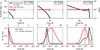 |
Fig. 2 Top: conditional halo mass functions from our sampler at z = 10 (solid black line) and the Sheth-Tormen CHMF (Equation (3), shown as a blue dotted line) in 10 000 under-dense (left, δ = −0.9) mean density (middle, δ = 0.0) and over-dense (right, δ = 1.4) Lagrangian cells of volume (2 Mpc)3 . Their ratio is indicated on the right vertical axis and shown as a solid red line which follows the target of unity (red dotted lines). Bottom: distribution of the number of halos (red curve) and total mass of halos (black curve) within each cell. The average of the distribution and the expected average from the Sheth–Tormen CHMF are shown as solid and dotted vertical lines, respectively. The agreement between the mean computed from samples and the target mean is evidenced by the overlapping solid and dotted lines. |
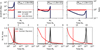 |
Fig. 3 Same as Figure 2, but sampling from 10000 descendant halos of mass 109, 1010, and 1011 M⊙ from redshift zdesc = 6 to the progenitor redshift, zprog = (1 + zdesc)∆z - 1, where ∆z = 1.02. Samples drawn from descendant halos use the mass-limited sampling described above, rather than the number-limited sampling used for the cells. The short time step results in a very tight distribution of total progenitor mass, although the number of halos and their mass distribution can vary significantly between individual descendants. |
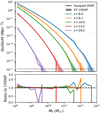 |
Fig. 4 Correlated sampling of halos from z = 6 to z = 30 within a 300 cMpc box. Top: total halo mass function within the box at from redshifts z = 6 to z = 30, compared to the Sheth-Tormen unconditional mass function represented as a shaded region with Poisson uncertainty. The black dotted line corresponds to a number density of one halo in the simulation volume within that bin. Bottom: ratio of the sampled mass function to the expected Sheth–Tormen unconditional mass function, showing an excess of small halos at the highest redshifts, but remaining within Poisson errors over the vast majority of masses and redshifts. |
3 Populating halos with galaxies
Assigning galaxies to host dark matter halos is a difficult task, especially at high redshifts where observational data are relatively sparse and the physics of star formation, feedback, and galaxy evolution is even more uncertain. Current approaches typically rely either on hydrodynamic simulations, semi-analytic, or semi-empirical models. Each have their own benefits and drawbacks.
Hydrodynamic simulations are appealing due to the fact that they capture gas dynamics and the gravitational interplay of baryons and dark matter. However, cosmological simulations cannot resolve individual star formation events and the associated feedback; therefore, they must rely on resolution-dependent sub-grid prescriptions that are calibrated against observations. Unfortunately, the predictions of such sub-grid recipes can vary dramatically in the regime where there is currently no data (e.g. Ni et al. 2023; Lovell et al. 2024). They are also numerically expensive and so cannot be directly used in an inference framework.
Semi-analytic models (SAMs), on the other hand, connect galaxies to halos using analytic equations for gas cooling, star formation and feedback (e.g. Croton et al. 2016; Mutch et al. 2016; Hutter et al. 2021). They are reasonably fast to evaluate. However, they typically include several ‘baked-in’ assumptions that might not hold for high-redshift galaxies, such as spherical symmetry, rotation-supported disks, and so on. Moreover, the free parameters of a given SAM can be difficult to interpret and generalise for other modelling procedures.
Semi-empirical models use parametric relations to connect galaxies to halos, fitting these relations to available data (e.g. Vale & Ostriker 2006; Behroozi et al. 2019; Park et al. 2019). This makes them fast and generalizable, at the cost of losing direct insight into the physics regulating star formation and galaxy evolution. Moreover, there is no unique choice of which relations to parametrise and which functional forms to use with them. As 21cmFASTv4 is intended to be used in a forwardmodelling framework, we have several requirements for our halo–galaxy connection:
- (i)
Speed – it must be fast enough for Bayesian inference;
- (ii)
Transparency – the galaxy–halo connection should be explicitly-defined, facilitating transparency of the model and its assumptions;
- (iii)
Flexibility – given our relatively poor knowledge of star formation and galaxy evolution in the first billion years, our model should be flexible enough to capture a large range of scenarios;
- (iv)
Generalizability – the galaxy–halo connection should be made in a ’universal language’ that can accommodate diverse theoretical models as well as observations, allowing us to set well-motivated priors on its free parameters.
To accommodate these requirements, we adopt a semi-empirical approach, but one that is anchored to well-studied galaxy scaling relations. Specifically, we define conditional probability densities that stochastically connect galaxy properties to host halo masses. These include the stellar-to-halo mass relation [SHMR; P(M* | Mh)], the star forming main sequence [SFMS; P(SFR | M*, z)], fundamental mass metallicity relation [FMR; P(Z | M*, SFR)], and the X-ray luminosity to star formation rate [LxSFR; P(LX | SFR, Z)]14. Sampling from conditional probability distributions is extremely fast, easy to interpret, flexible, and allows us to characterise a wide range of theoretical models and observational data. Ultimately, we want to infer the parameters of these distributions (e.g. means, scatters, temporal correlations, etc.) from multi-tracer observations15, using prior ranges informed by both simulations and low-redshift observations. These inferred properties of the unseen first galaxies can subsequently be interpreted using dedicated galaxy simulations and models, in an analogous manner to how we interpret direct observations of local galaxies. We present our approach in detail below.
After the halo masses are calculated for a snapshot, we assign galaxy properties to each halo by sampling from conditional distributions with free parameters governing their means and scatters. Our distributions for each property are taken mostly from Nikolic´ et al. (2024), with small differences which are detailed below. The stellar mass, star formation rate, and X-ray luminosity of each halo are sampled from separate log-normal distributions,
![Mathematical equation: P(\log(x))\,{=}\,\mathcal{N} (\mu_{\log x},\sigma_{\log x})\,{=}\,\frac{1} {\sigma\sqrt{2\pi}}\mathrm{exp} \left[ -\frac{1}{2}\left( \frac{\log(x) - \mu_{\log x})}{\sigma_{\log x}} \right)^2 \right] ,](/articles/aa/full_html/2025/09/aa54951-25/aa54951-25-eq8.png) (7)
(7)
where x is the halo property of interest, while μlog x and σlog x are the mean and standard deviation of the logarithm of the property. It is noteworthy that the log-normal distribution is asymmetric, and the mean value of a variable drawn from the distribution is given by  (see Appendix B of Nikolic et al. 2024). In order to avoid a parametrisation scheme where changing the amount of scatter drastically alters the mean properties, by default we define our scaling relations in terms of their means μx, rather than their mean logarithms μlog x as is the standard for observational fits. However, we investigate the latter models, which do not have a normalised mean, in Section 6.
We assign a correlation ρlog x between progenitor and descendant properties dependent on the redshift step via a free parameter, Cx,
 (8)
(8)
To generate samples with the target correlation, mean, and variance, we sample each progenitor property log(xp) from the conditional bivariate Gaussian distribution given the descendant property log( xd)16, which itself is a Gaussian,
 (9)
(9)
where subscripts p and d mark means and variances calculated using progenitor and descendant properties respectively. In the limiting case of ρlog x = 0, log(xp) is simply sampled from N(μlog x,p,σlog x,p) uncorrelated from its descendant. In the case of ρlog x = 1, it is mapped directly from log(xd), adjusting for the differences in mean and variance between the two distributions.
We parametrise the mean and scatter of each conditional probability distribution using physically or empirically motivated functional forms. The mean stellar mass at fixed halo mass, μ*, is set by the following scaling relation (Mirocha et al. 2017):
 (10)
(10)
where fi,10 is the value of the SHMR at 1010 solar masses, and α* is its low-mass power-law slope. We include an additional high-mass power-law component compared to Park et al. (2019), where the SHMR transitions to a power-law slope of α*2 at a pivot mass of Mpivot. Previously, in 21cmFAST it was not important to include a separate high-mass slope in the SHMR since halo masses above Mh ≳ 1011 M⊙ are too rare to contribute significantly to reionisation in data-constrained models (e.g. Qin et al. 2025). Here however we include the turnover since 21cmFASTv4 is intended to forward-model galaxy surveys that can only observe such rare, bright galaxies (Gagnon-Hartman et al. 2025). The characteristic halo mass below which star formation is exponentially suppressed, Mturn, can either be used as a free parameter or it can be modelled as the largest of three physical scales (cf. Qin et al. 2020): (i) MSNe, a free parameter corresponding to disruption from supernovae feedback; (ii) Mcool, a redshift-dependent atomic-cooling threshold corresponding to a virial temperature of 104 K; and (iii) Mphoto, a characteristic scale set by photo-heating feedback that depends on the local reionisation redshift and ionising background of each cell (Sobacchi & Mesinger 2013). The standard deviation in the log stellar-to-halo mass ratio σ* is a free parameter, set in our fiducial model to a constant 0.3 dex, roughly motivated by the results of hydrodynamic simulations (e.g. Hassan et al. 2022; Nikolic´ et al. 2024).
The mean star formation rate (SFR) is determined by the following relation from Park et al. (2019):
 (11)
(11)
where M* is the stellar mass of the galaxy (sampled from P(M*|Mh) as discussed above) and t* is a free parameter corresponding to the characteristic star formation time-scale in units of the Hubble time 1/H(z) (which also scales as the halo dynamical time during matter domination). We allow for a parametric scatter around the mean SFMS, which by default decreases with increasing stellar mass according to a power-law:
 (12)
(12)
Here, σSFR,lim is the high-mass limit of the SFMS scatter, and σSFR,idx is its power-law index with stellar mass.
Finally, the mean rest-frame soft-band (with photon energies less than 2keV) X-ray luminosity per unit star formation, LX,<2keV, of high-redshift galaxies is modelled as a double powerlaw dependent on the SFR and stellar mass, via the gas-phase metallicity, Z,
 (13)
(13)
where Z is calculated using the FMR presented in Curti et al. (2020), and subsequently adjusted for redshift evolution (Curti et al. 2024):
 (14)
(14)
where
 (15)
(15)
We use a double power-law to be consistent with high-metallicity measurements from Brorby et al. (2016) with a flattening of LX,<2keV/SFR at low metallicities (e.g. Fragos et al. 2013; Lehmer et al. 2021; Kaur et al. 2022; Geda et al. 2024). We assume the specific X-ray luminosity is a power-law with photon energy LX ∝ E−αX, where αX is the spectral index of X-ray sources. The luminosity is normalised such that its integral is equal to the soft-band luminosity sampled above
 (16)
(16)
where E0 is the energy threshold above which X-rays can escape their host galaxies. Here, use a fiducial value of E0 = 0.5 keV, motivated by hydrodynamic simulations of the first galaxies (Das et al. 2017).
While the temporal auto-correlation lengths, Cx, are free parameters within 21cmFASTv4, their main purpose is to ensure that the variation in halo properties does not depend on the length of the simulation time-step. Default values for C* and CSFR were set to be roughly consistent with simulated galaxies in Astrid (Bird et al. 2022). We leave the exploration of these parameters to future work. We note that such random sampling can in some cases result in an unphysical decrease in the stellar mass or metallicity of a descendant compared to a progenitor. Due to memory constraints, we do not explicitly disallow such trends although we note that the summation of galaxies within a cell, the correlation coefficients, and the growth of halos over time all combine to minimise the occurrence of such unphysical behaviour. Indeed we find no discernible impact on power spectra, luminosity functions or global histories when we vary C* = (0,0.5,5.0). Future versions of the model will include a more robust tracking of progenitor-descendant connections which will completely disallow any such unphysical trends.
In contrast to Nikolic´ et al. (2024), we do not include scatter around the FMR, since this scatter was found to be sub-dominant in determining all radiation fields. At this stage, we also do not include scatter in the ionising escape fraction, as there is currently no consensus on how to parametrise it (e.g. Yeh et al. 2023; Kreilgaard et al. 2024). Furthermore, scatter in the escape fraction is unlikely to impact large-scale radiation fields unless there is a strong dependence on galaxy properties (e.g. Hassan et al. 2022; Nikolic´ et al. 2024). Instead, we use the Park et al. (2019) relation for the mean escape fraction, which scales with halo mass as
 (17)
(17)
which allows us to compute the cumulative number of ionising photons that escaped from a given halo as
 (18)
(18)
where we take the number of ionising photons per stellar baryon Nγ = 5000 for use in the excursion-set reionisation algorithm.
We list our galaxy parameters and fiducial values in Table 1. These fiducial values are used throughout this paper except where otherwise indicated. Coefficients represented as numbers in the above equations are currently fixed in our model.
21cmFAST includes an optional prescription for star formation inside molecularly cooled galaxies (MCG; cf. Qin et al. 2020), which could have an independent SHMR, expressed as
 (19)
(19)
Overall, MCGs are allowed to have different escape fractions when calculating the ionisation field, as well as different spectra based on population III stellar models. The atomic cooling threshold mass Mcool acts as an upper turnover mass, which separates this population from the atomically cooled galaxies (ACG’s), while MLW is the lower turnover mass, set by inhomogeneous Lyman-Werner radiation feedback and the relative velocities between dark matter and baryons. When the minihalo component is enabled by the user, the discrete halo model samples the MCG component from a log-normal distribution of the same width σ*, but with a mean set by Equation (19), analogously to the ACG component. The specific star formation rates for MCGs are sampled from the same distributions as for the ACGs. Metallicities and X-ray luminosities are based on the combined stellar mass and star formation rate of both ACGs and MCGs. While we do not include MCGs in this work, they are available within 21cmFASTv4 with the full functionality implemented initially by Qin et al. (2020) and expanded upon in Muñoz et al. (2022).
To demonstrate the flexibility of our model, in Figure 5 we show two different parameter combinations capable of capturing the SHMR and SFMS seen in two different hydrodynamical cosmological simulations: the zoom-in suite SERRA (Pallottini et al. 2022) (setting f*,10 = 0.16, α* = 0.1, t* = 0.13) and the large cosmological simulation Astrid (Bird et al. 2022) (setting f*,10 = 0.005, α* = 0.65, t* = 0.13). While the simulations are roughly consistent at the highest halo masses, they diverge significantly at low halo masses, where there are no direct observations to anchor their sub-grid prescriptions. Our prescription is able to characterise such diverse distributions of galaxy properties, computing the corresponding signatures of their radiation imprints in the IGM. We illustrate such an approach in more detail in Section 7.
Fiducial parameters for galaxy scaling relations used in Equations (7) to (17).
4 Calculating radiation fields
The galaxy sampling method described in Sections 2 and 3 forms a new source model in 21cmFASTv4. Full halo mass histories are generated prior to calculating any radiation fields, moving backward in time in a user-defined redshift range. Each halo is moved from Lagrangian to Eulerian space, together with the matter field, using 2LPT. We then grid the galaxy source field, starting from the highest redshifts, computing inhomogeneous radiation fields and taking into account feedback from previous time-steps (Sobacchi & Mesinger 2013; Qin et al. 2020; Muñoz et al. 2022).
The X-ray and Lyman alpha specific intensities (JX, Jα) at redshift, z, and frequency, ν, is computed by integrating back along each cell’s lightcone as
 (20)
(20)
where x is the cell’s location, εi is the specific comoving emissivity at a location x′, redshift z′, and emitted frequency ν′ = ν(1 + z)/(1 + z′). The optical depth, τi, accounts for attenuation due to the intervening IGM17. Wts(x′, z, z′) is a window function which selects sources at the correct distance from x, given z and z′. Heating and ionisation rates are then computed by integrating Ji over ν, and relevant cross-sections. Finally, the residual ionisation by X-rays, kinetic temperature, and spin temperature of the mostly neutral hydrogen are determined from these rates. Further details on these models, including how emissivities εi are calculated from star formation rates of ACGs and MCGs, and how IGM attenuation is computed can be found in Mesinger et al. (2011); Sobacchi & Mesinger (2013); Qin et al. (2020) and Muñoz et al. (2022).
In the previous versions of 21cmFAST, when computing the emissivity at a comoving distance R(z, z′), the Eulerian overdensity was evolved back from z via the ratio of linear growth factors, D(z′)/D(z) and the window function Wts(x′, z, z′) was a spherical top-hat. This was done to speed up the calculation as both the absorbing IGM and emitting galaxies were calculated directly from density fields pre-filtered with the same window functions. With the discrete source field in 21cmFASTv4, we can directly use the previous inhomogeneous emissivity fields εi(x, z′(R)) and a spherical shell filter of finite width.
 (21)
(21)
where Ri and Ro are the inner and outer comoving radii of the shell respectively18. For computational efficiency, we apply this filter to our gridded emissivities in Fourier space, using its Fourier transform:
![Mathematical equation: \begin{multline} W_\mathrm{ts}(k,R_\mathrm{i},R_\mathrm{o}) = \frac{3}{k^3(R_\mathrm{o}^3 - R_\mathrm{i}^3)} \{ [\sin(kR_\mathrm{i}) - kR_\mathrm{i} \cos(kR_\mathrm{i})] \\- [\sin(kR_\mathrm{o}) - kR_\mathrm{o} \cos(kR_\mathrm{o})] \}. \end{multline}](/articles/aa/full_html/2025/09/aa54951-25/aa54951-25-eq24.png) (22)
(22)
Because the mean free path of Lyman limit photons through the neutral IGM is very short, reionisation is a fairly local process with sharp discontinuities along ionisation fronts, and is therefore not well captured by the lightcone integration of Equation (20). Instead, reionisation is calculated via the excursion set algorithm (Furlanetto et al. 2004; Zahn et al. 2011; Mesinger et al. 2011), where the source field is filtered on a series of decreasing radii, marking as ionised those cells that receive more ionising photons than neutral atoms19 plus recombinations,
 (23)
(23)
where the left-hand side is the number of ionising photons reaching a cell, directly calculated from the cumulative ionising photon number, nion (see Equation (18)) using a filter function Wion(r, R) dependent on the distance between the source cell and absorber cell r = |x′ - x| and nrec is the number of recombinations that have occurred within the cell. In previous versions of the code we used a spherical top-hat or sharp-k filter for Wion(r, R), with the maximum allowed scale set by the mean free path through the ionised medium, λlls. Since we use a discrete ionising source field, here we implement the exponential window function suggested by Davies & Furlanetto (2022) (their MFP – ε(r) method):
 (24)
(24)
Here, we take λlls = 25 cMpc/h, based on Lyman limit system measurements at z ≲ 5 (Songaila & Cowie 2010). This parameter can also be varied, though for simplicity we take a fixed value in this work20.
Once the thermal and ionisation state of the gas is determined by the above models, we compute the 21cm signal in the form of the differential brightness temperature dTb (e.g. Furlanetto et al. 2006)
 (25)
(25)
where Tγ is the temperature of the cosmic microwave background and each cell is described by its overdensity, δ, neutral fraction, xHI, spin temperature, Ts, and line-of-sight velocity gradient,  . Then, dTb quantifies the difference in intensities of the IGM against the cosmic microwave background at the rest frame wavelength of 21cm.
 |
Fig. 5 Distributions of stellar to halo mass (top) and star formation rate to stellar mass (bottom) at z = (6.0,7.7,12). Orange and blue points correspond to galaxies taken from two hydrodynamical simulations: the zoom-in simulation suite SERRA (Pallottini et al. 2022) and the large cosmological simulation Astrid (Bird et al. 2022). For the SERRA sample we plot every central galaxy at these redshifts, while for Astrid we plot a subsample randomly selected in fixed logarithmic mass bins. Both codes have been calibrated to reproduce observable data at Mh ≳ 1012M⊙, but predict very different SHMRs for the unseen, faint galaxies that dominate the EoR and CD. The orange and blue contours correspond to two different parameter combinations in 21cmFASTv4 whose conditional distributions can characterise the correspondingly-coloured galaxy populations from the different hydro codes. These contours correspond to 2-5 σ of the joint distributions, P(M*, Mh) and P(SFR, M*), highlighting how the vast majority of galaxies are expected to be far below the resolution limits for large-scale cosmological simulations. This figure demonstrates that our semi-empirical model is flexible, capable of capturing a large range of predictions, and eventually allowing us to infer such galaxy properties from multi-tracer galaxy and IGM observations. |
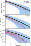 |
Fig. 6 Galaxy properties within 323 Lagrangian cells with side length 2 Mpc at exactly mean density (δcond = 0), including stochastically sampled halos above 108 M⊙ showing the variance in galaxy properties solely from the sampling of halo populations and galaxy properties. We show halo mass density (top), cumulative ionising photon density per hydrogen atom (middle) and X-ray soft-band emissivity (bottom). Solid and dotted black lines show the mean and median of the distribution respectively, and green lines show the expected mean obtained by integrating the CHMF. Blue shaded regions span the [2.5, 97.5] percentile range, and the thin red lines show 32 randomly selected individual cells. Changes over time in the summed galaxy properties are caused by the growth of halos, as well as the variability in the stellar to halo mass ratio and specific star formation rate. |
5 Illustrative examples
To showcase some novelties of this model, we performed simulations using the halo sampler described in Section 2, galaxy property distributions described in Section 3, and EoR/CD model described in Section 4. All astrophysical parameters for this run are laid out in Table 1. Firstly, in Figure 6 we show the redshift evolution of the density of the total halo mass above 108 M⊙, cumulative ionising photon density per hydrogen atom, and the rest-frame soft-band X-ray emissivity for a test case of 323 Lagrangian cells of side length 2 Mpc at exactly cosmic mean density. Despite having the same density by construction, each cell can vary greatly in its properties as new galaxies form and experience periods of high or low star formation.
Next, we performed a full simulation with side-length 300 Mpc from z = 35 to z = 5. Initial conditions are sampled on a 6003 grid, which is downsampled to 1503 for the purposes of sampling halos as well as performing the 2LPT and IGM calculations. We integrate the average CHMF in the range 107 M⊙ < Mh < 108 M⊙, and perform stochastic sampling above 108 M⊙. We show how the 21cm signal is affected by the spatial distribution of galaxies at three key epochs in Figure 7. At each of these epochs, the changes in the IGM are being driven by cosmic radiation fields sourced by galaxies (see, e.g. Furlanetto et al. 2006). At z = 14.8 the 21cm cold spots are close to the brightest galaxies, as Lyman alpha radiation couples the spin temperature to the kinetic temperature which is below the CMB temperature at the time. Around z = 9.0 areas close to galaxy overdensities have a higher 21cm brightness temperature, as X-rays from nearby sources heat the IGM. Finally during reionisation at z = 7, the coldest regions are again near galaxy overdensities, as they have ionised their surroundings resulting in a brightness temperature close to zero. Although the cosmic radiation is dominated by the more abundant, faint galaxies not visible in the figure, they cluster around the brightest galaxies denoted with green circles, allowing us to see these spatial correlations between bright galaxies and IGM properties.
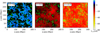 |
Fig. 7 Co-location of galaxies and the 21cm brightness temperature fields in our illustrative simulation during key stages in the history of the CD and EoR. We show slices at z = 14.8, z = 9.0, and z = 7.0, corresponding to epochs of Lyman alpha coupling, X-ray heating, and reionisation, respectively. Green circles denote 200 galaxies with the brightest UV magnitudes in each slice, with larger circles corresponding to brighter galaxies. |
6 Impact of stochasticity on the 21cm signal
Our new simulations allow us to quantify the importance of stochasticity in both the halo field as well as the halo-galaxy connection. To showcase this, we ran five iterations of 21cmFASTv4, all using the same Sheth–Tormen halo mass function and a box side-length of 300 Mpc. Initial conditions are sampled on a 6003 grid, while the galaxy, IGM, and radiation fields were computed on 2003 grids. Astrophysical parameters are as presented in Table 1, with two exceptions: the mean X-ray luminosity at fixed star formation rate, which is set to a constant LX/SFR = 1040 ergs−1M⊙−1yr, and the SHMR is confined to a single power-law, effectively setting α*2 = α* = 0.5. Additionally, we switched off the mean-free path filter described in Section 4 and Davies & Furlanetto (2022), using a spherical top-hat ionisation filter for all simulations. These changes were made for easier comparison with 21cmFASTv3 and to highlight the effects of the stochastic halo field.
The first iteration titled ‘v3 Default’ shows the previous default source model, in which the galaxies are not localised but instead mean abundances are calculated from CHMFs in expanding spherical volumes centred on each cell. The second run titled ‘CHMF on Grid’ has a fixed, one-to-one relationship between the source grid and the evolved density grid based on the integral of the conditional mass function on the scale of a grid cell. The emissivity fields produced from this are then filtered in the same way as the sampled halo fields21. As in 21cmFASTv3, both the ‘CHMF on Grid’ and ‘v3 Default’ models have their global mean emissivities at each wavelength fixed to the expected mean, which is obtained by integrating the unconditional mass functions at each redshift. The third iteration titled ‘v4 no astro scatter’ uses our halo sampler (described in Section 2); however, with no log-normal scatter around the galaxy scaling relations, as described in Section 3 (by setting σ* = σSFR,lim = σSFR,idx = σX = 0). The fourth and fifth iterations ‘v4 Mean Norm’ and ‘v4 No Mean Norm’ both use the halo sampler with log-normal scatter in galaxy properties. The key difference between these two models is whether the scaling relations (Equations (10), (11), (13), and (19)) are defined to have a fixed mean as the scatter increases22. In ‘v4 No Mean Norm’, the mean log-log scaling relation is kept fixed and, therefore, as log-normal scatter is increased, the linear mean increases (cf. Appendix B in Nikolic´ et al. 2024). In ‘v4 Mean Norm’ on the other hand, the linear mean is kept constant as the scatter is changed.
The key differences between each model are summarised in Table 2. The 21cm brightness temperature lightcones are shown in Figure 8. In Figure 9 we plot the spherically-averaged 21cm power spectra  at three epochs: the midpoint of the EoR (
 ) is shown in the bottom panel, the epoch of heating when the mean brightness temperature is zero (
 ) is shown in the middle panel and Lyman alpha coupling (when
  is at its minimum) is shown in the top panel.
Comparing the ‘v3 Default’ and ‘CHMF on Grid’ outputs highlights the impact of defining the source model only at the cell scale, rather than over a range of larger spheres. Indeed ‘CHMF on Grid’ is a notable outlier between our various test cases (aside from ‘v4 No Mean Norm.’ which is discussed below), having patchier heating and ionisation morphologies characterised by larger ionised and heated regions. Applying CHMFs only on relatively small Lagrangian scales corresponding to the simulation grid would miss the most massive halos (e.g. Barkana & Loeb 2004; Appendix A in Nikolic´ et al. 2024). Attempting to correct for this by instead conditioning the HMFs on the evolved (Eulerian) cell densities (i.e. CHMF on Grid), overcompensates and instead results in spuriously massive halos in the densest cells (e.g. footnote 4 in Sobacchi & Mesinger 2014; Fig. 13 in Trac et al. 2022). This results in ‘CHMF on Grid’ overestimating the 21cm large scale power, as seen in Figure 9.
Comparing the ‘v3 Default’ and ‘v4 No Astro Scatter’ illustrates the importance of having a stochastic halo finder in the source model. Understandably, having discrete sources results in small-scale ’shot-noise’ in the power spectra, as seen in Figure 9 at k ≳ 1 Mpc−1. During the EoR, differences on larger scales and from visual inspection of the lightcones are modest, while moderate to large scale power is reduced by ~50% during Lyman alpha recoupling and X-ray heating, due to the fact that including scatter decreases the effective bias of the source population during these epochs.
Comparing instead ‘v4 No Astro Scatter’ to ‘v4 Mean Normalisation’ isolates the importance of astrophysical scatter in our default model, at fixed mean emissivities. We see that when the emissivities are adjusted to have the same mean, the scatter in galaxy properties has a negligible impact on the 21cm signal. This is due to the fact that variations in halo mass distribution cause a much wider scatter (>1dex) in emissivities at fixed matter overdensity, such that they dominate when added in quadrature to the scatters in the galaxy properties ≤0.5 dex. The relative importance of scatter in halo abundances versus astrophysics will depend however on the details of the model and sampling method, and any choice that reduces the variance in the halo mass distribution (such as the stricter halo mass conservation criteria in Nikolic´ et al. 2024 which limits the total halo mass variation within a 5 Mpc region to ±10%) will increase the relative importance of astrophysical scatter.
However, if we are including scatter around log-normal galaxy scaling relations, without adjusting the means of the distribution, the resulting impact is significant. We can see this comparing ‘v4 Mean Normalisation’ with ‘v4 No Normalisation’. The milestones of the 21cm signal in the later model are shifted to earlier times, because of the shift in the mean when widening a log-normal distribution. The most dramatic shift, resulting in a large increase in power (cf. Figure 9), occurs during the X-ray heating epoch. Compared to the UV emissivity, the X-ray emissivity is sensitive to an additional source of scatter coming from the P(LX|SFR, Z) distribution. This serves as a caution against using empirically-derived mean log-log scaling relations directly in theoretical models without accounting for scatter around the mean (see also Nikolic´ et al. 2024).
As mentioned before, the astrophysics of EoR/CD galaxies is very poorly known, and our conclusions could depend on our choice of fiducial parameters. Our fiducial parameters characterising the halo–galaxy connection were loosely motivated by hydrodynamic cosmological simulations. However, output from different simulations can disagree significantly (e.g. the two simulations shown in Figure 5 have mean SHMR that are different by up to two orders of magnitude). Moreover, recent observations of UV luminosity functions at z > 11 using JWST are difficult to explain with current simulations and might require significantly more scatter in galaxy properties (e.g. Pallottini & Ferrara 2023; Gelli et al. 2024; Nikolic´ et al. 2024).
Here, we show how increasing (or decreasing) the level of astrophysical scatter impacts observables. We performed runs with two or three times the scatter of our fiducial runs, where a × Y boost corresponds to substituting σlog x → σlog x + log Y in each of our scaling relations. As with the previous simulations, we included runs where the galaxy scaling relations define a fixed mean and those where the mean is allowed to increase with the log-normal scatter. The power spectra from these runs at the same two epochs as in Figure 9 are shown in Figure 10.
In the case where the mean of the galaxy property distributions are not fixed, there is significant change in the power spectrum at all epochs driven by an increase in the mean stellar mass, star formation rate and X-ray luminosity. This mean shift causes reionisation and reheating to progress faster, resulting in a higher power on all scales simply due to the higher redshift. In the case where the galaxy scaling relations define a fixed mean, we begin to see a ~10% increase in 21cm power during X-ray heating at ≳2× fiducial scatter, and a ~50% increase for 3× fiducial scatter. At these increased levels, the astrophysical scatter begins to dominate over the scatter introduced by the halo sampling, and the 21cm signal can be used to constrain the width of galaxy property distributions.
Although our fiducial level of scatter has little effect on the 21cm power spectrum, it leaves a significant imprint on the UV luminosity function, as shown in Figure 11. Simply adding lognormal scatter to a scaling relation without keeping the means fixed drives up the UV luminosity function at all magnitudes. When normalised to have the same mean galaxy properties, the UVLF flattens as scatter increases, resulting in a factor of 10 increase in the abundance of bright galaxies, MUV ~ −22. By utilising observables from both the IGM and galaxies, we will be able to constrain the normalisation and scatter in bulk galaxy property distributions.
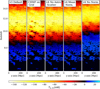 |
Fig. 8 21cm brightness temperature lightcones from four runs of 21cmFAST. From left to right: ‘v3 Default’ shows the previous default model, where the source field is calculated on the filtered density grids, ‘CHMF on Grid’ shows a model where there is a one-to-one relationship between cell density and emissivities, based on the integral of the CHMF; ‘v4 No Astro Scatter’ shows the effects of our halo sampler described in Section 2, without any stochasticity in the galaxy properties. We show two cases for the model with stochasticity in the halo mass distribution and galaxy properties, which differ in their interpretations of the scaling relations; ‘v4 Mean Norm’ shows the case where the scaling relations are defined by the mean of each property’ and ‘v4 No Norm’ shows the case where the scaling relations are defined by the mean logarithm. In the latter case, increasing the log-normal scatter also increases the mean emissivities at all wavelengths. |
Settings of the simulations performed to investigate the effect of stochasticity in halo masses and bulk galaxy properties.
 |
Fig. 9 21cm power spectra shown for the same five models as in Figure 8. We show the power-spectra at two points in cosmic history: the midway point of the EoR (the snapshot at which the total ionised fraction is closest to 50%), as well during X-ray heating where the volume-weighted mean brightness temperature |

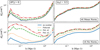 |
Fig. 10 21cm brightness temperature power spectra from 21cmFASTv4 runs with differing levels of astrophysical scatter. The top rows show the runs where the scaling relations have a fixed (linear) mean as scatter increases, whereas the bottom rows show runs where the mean is allowed to increase with the scatter (i.e. at a fixed log-log mean relation). The left column shows the epoch during X-ray heating where |


7 Forward modelling multi-tracer data
The halo sampler described in Section 2 combined with the flexible halo–galaxy connection described in Section 3 form a new optional source model in 21cmFASTv4. In this set-up, multiwavelength radiation sources are explicitly localised, and have their properties sampled self-consistently according to given distributions. Any additional quantities such as line luminosities can be easily calculated in post-processing from either the gridded galaxy fields or catalogues. Our simulations can thus self-consistently compute lightcones of galaxies, their radiation fields and the corresponding IGM evolution. These can be used to forward model IGM observations, galaxy surveys, LIMs, as well as their cross-correlation allowing us to infer cosmological parameters or those characterising the halo–galaxy connection (e.g. Figure 1).
We show the full lightcones of overdensity, cumulative ionising photon density, soft-band X-ray emissivity, 21cm brightness temperature, and CII surface brightness density from 21cmFASTv4 with our fiducial parameters (Table 1) in Figure 12. We calculate the latter using the following simple linear relation (De Looze et al. 2014) for CII luminosity for all galaxies as
 (26)
(26)
We summed all sources within each cell to obtain the final surface brightness density, assuming for simplicity that all galaxies are at the centre of the cell, expressed as
 (27)
(27)
where ∆ν is the frequency width of the cell in GHz, Ω is the angular size of the cell and DL is the luminosity distance in Mpc.
As a simple demonstration of such a multi-tracer approach, we ran two simulations with the same dimensions, mass function, and sampling algorithm as those in Sections 5 and 6, but with two sets of astrophysical parameters chosen to characterise simulated galaxies from SERRA (Pallottini et al. 2022) and Astrid (Bird et al. 2022). As discussed in Section 3, this was done by setting the parameters related to the SHMR and SFMS to be consistent with the distributions from each simulation. In the case of SERRA, we used f*,10 = 0.16, α* = 0.1, and t* = 0.13, and in the case of Astrid we use f*,10 = 0.005, α* = 0.65, and t* = 0.13. Both runs have their escape fractions tuned so that reionisation finishes around z = 5.5, with all other parameters set according to Table 1. By construction, both models are consistent with current galaxy observations. However, they imply very different star formation efficiencies in the abundant faint galaxies below direct detection limits. Thus, these two galaxy formation scenarios would result in very different cosmic radiation fields, and IGM and/or LIM observations could be used to distinguish between them. We illustrate this in Figure 13 where we compute the 21cm brightness temperature fields and CII line intensity maps corresponding to these two models.
The vastly different stellar populations between these models are easily distinguished in the X-ray heating history, with the more efficient star formation of SERRA suggesting the epoch of heating occurs at z ∼ 13, while our Astrid-like galaxies imply it occurs at z ∼ 8.
Even with a similar reionisation timing, we can clearly distinguish these scenarios in the auto and cross power spectra of 21cm brightness temperature and CII surface brightness density. We define the auto and cross power spectra as
 (28)
(28)
 (29)
(29)
 (30)
(30)
where  . The flatter stellar-to-halo mass relation in the run matched to SERRA means that less-massive halos have a more dominant contribution to cosmic radiation fields. This results in smaller HII regions meaning higher power at large k (e.g. McQuinn et al. 2007), a less biased CII surface brightness density field, as well as a stronger anti-correlation between 21cm and CII on small scales.
This example shows the effect of changing parameters related to one of our galaxy scaling relations on two observable probes. When considering all of our scaling relations, it is important to note that some parameters controlling the galaxy properties can have degenerate effects on certain observables (for example, the SHMR and the escape fraction normalisations will have a degenerate effect on global reionisation history). These degeneracies must be broken by comparing our models to multiple observables at multiple redshifts. Our new framework allows us to perform inference on the global 21cm signal, 21cm power spectrum, galaxy luminosity functions, line intensity maps, and radiative backgrounds simultaneously, including their cross-correlations. As a result, we will be able to obtain much tighter constraints on the physics driving the first galaxies and their effects on the IGM.
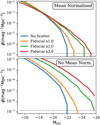 |
Fig. 11 UV luminosity functions at z = 8 by setting the scatter in the galaxy properties to either zero (blue line), equal to the fiducial values from Table 1 (orange line), and increased by factors of 2 (green line) or 3 (red line). Top: runs where the scaling relations are normalised to have the same linear mean. Bottom: runs where log-normal scatter is simply added to a fixed log-log mean relation. In both cases increasing scatter results in a flattening of the relation; however, in the later case it also results in significantly brighter galaxies overall. |
8 Conclusions
In this paper, we introduce a fast and flexible method for producing galaxy populations within the semi-numerical cosmological simulation code 21cmFAST. Dark matter halos are identified using a combination of previous Lagrangian halo finding and a new, efficient merger-tree algorithm. Galaxies are assigned to dark matter halos using flexible conditional probability distributions, motivated by well-established empirical relations. Radiation fields are computed using these discrete galaxy source fields, including also the mean contribution of unresolved sources in each grid cell if the user selects a low halo mass resolution. The model can produce stochastic halo populations and associated EoR/CD history down to 108 M⊙ in a 300 Mpc lightcone from z = 35 to z = 6 in approximately 3 core hours. This can be reduced even further by raising the halo mass threshold for the sampler, while assuming mean emissivities for the unresolved galaxy component.
The model features parameters controlling the mean and scatter in the galaxy scaling relations, resulting in a wide range of possible scenarios for the co-evolution of galaxies and the IGM during cosmic dawn and reionisation. We show that our parametrisation is sufficiently flexible to characterise the galaxy properties predicted by very different hydrodynamic simulations. Additionally, 21cmFASTv4 is now able to output galaxy properties in the form of both halo catalogues and gridded halo properties. Statistics calculated from the galaxy field can be easily produced and corresponding observations can be used in our inference pipelines, allowing us to tighten constraints on our model parameters and use cross-correlations to probe the galaxy-IGM connection.
We find that the stochastic source field produces significant shot-noise in the 21cm power spectrum at all redshifts. At our fiducial levels, the 21cm power-spectrum is unaffected by the scatter in the stellar-to-halo mass relation, star-forming main sequence, and X-ray luminosity, as scatter is dominated by stochasticity in the halo mass distribution. However we still see their effects in the UV luminosity function, which flattens as the scatter in the scaling relations increases. Increased levels of astrophysical scatter, which may be implied by recent JWST observations (e.g. Mason et al. 2023; Shen et al. 2023; Nikolic´ et al., in prep.), can be constrained by the 21cm power spectrum if they are two to three times our fiducial levels.
Observables of the EoR and CD are highly complementary and by comparing a wide range of observations with models, we will be able to extract the maximum information from current and next-generation telescopes. We showcase an example of such synergies in the cross-correlation between the 21cm signal and CII line intensity maps, where we are able to easily distinguish between galaxy models implied by different hydrodynamic simulations.
Our simulator also facilitates modern inference techniques such as simulation-based inference (SBI). In a classical inference framework, it is necessary to explicitly define a likelihood function that would need to account for all high-order correlations between different tracers as well as different statistics of the same tracer. Such likelihoods are exceedingly difficult to define and common Gaussian assumptions can bias constraints (e.g. Prelogovic´ & Mesinger 2023). On the other hand, SBI takes advantage of self-consistent forward models of multi-tracer observables, allowing neural density or neural ratio estimators to be used for inference without specifying the likelihood explicitly (e.g. Alsing et al. 2018; Zhao et al. 2022; Saxena et al. 2023). Our simulator even enables ‘field-level’ SBI (cf. Triantafyllou et al., in prep.), bypassing the compression of fields into summary statistics such as power spectra or luminosity functions, and thus allowing us to take advantage of non-Gaussian features. It also allows us to jointly constrain the initial conditions of the observation volume (e.g. Jasche & Wandelt 2013; Savchenko et al. 2025). Our code is also modular, allowing the user to swap in different galaxy models and different radiative transfer algorithms. This will allow us to cleanly separate and explore the impact of assuming different galaxy models and different numerical RT implementations.
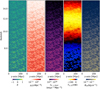 |
Fig. 12 Lightcones containing example outputs from 21cmFASTv4 with default parameters. The leftmost panel shows the evolved matter density field. The next two panels show gridded galaxy properties: cumulative ionising photon density per hydrogen atom and soft-band X-ray emissivity. The two rightmost panels show observables: the 21cm brightness temperature and CII surface brightness density. |
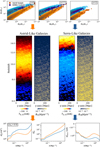 |
Fig. 13 Schematic showing how different galaxy populations affect IGM and LIM observables. Top: SHMR panels from Figure 5, where we set our galaxy scaling relations to be consistent with either the SERRA or Astrid cosmological simulations. Middle: resulting 21cm brightness temperature and CII surface brightness density lightcones in the range 6 < z < 16. Bottom: auto power spectra from both fields, as well as their cross power spectrum at the midpoint of reionisation |

Acknowledgements
We thank G. Sun for helpful comments on a draft version of this manuscript. We gratefully acknowledge computational resources of the HPC centre at SNS. AM acknowledges support from the Italian Ministry of Universities and Research (MUR) through the PRIN project ‘Optimal inference from radio images of the epoch of reionisation’, and the PNRR project ‘Centro Nazionale di Ricerca in High Performance Computing, Big Data e Quantum Computing’. SGM has received funding from the European Union’s Horizon 2020 research and innovation programme under the Marie Skłodowska-Curie grant agreement No. 101067043.
Data availability
21cmFASTv4 is made publicly-available at github.com/21cmfast/21cmFAST, as well as via PyPI as ‘21cmFAST’. Data files, including lightcones and parameter files for specific runs will be shared upon reasonable request to the corresponding author at This email address is being protected from spambots. You need JavaScript enabled to view it. . The runs may also be reproduced using approximately 3 core hours and less than 32GB of memory.
Appendix A Code timing and memory usage
In Figure A.1, we show the total runtime of a lightcone using halo sampler, versus the fixed halo grids (‘CHMF on Grid’ in Section 6) and the default excursion set source model at various box sizes. All boxes run from z = 35 to z = 6 and use a cell size of 2 cMpc. The halo sampler takes approximately double the runtime at all box sizes. The extra runtime is due in roughly equal parts to the halo sampler itself which performs calculations on a large number of halos, as well as the more complicated filter functions applied to the radiation fields (see section 4). This can be seen in the difference between the halo sampling run and fixed halo grid run, which still uses the new filters, but does not need to sample any halos. To mitigate the increased requirements of the halo sampler, we provide an option which adds the average contribution from halos below the minimum sampled mass to the gridded source properties, sacrificing stochasticity in the smallest halo masses allowing the user to set a higher minimum mass. This speeds up the simulation and lowers memory requirements without losing the contribution of smaller sources. Setting the minimum mass to 1010 M⊙ improves the runtime significantly, approaching the time taken by the fixed halo grid run.
The halo sampler also requires more memory than the default 21cmFASTv3 run, and is strongly dependent on the minimum halo mass. We show the memory required by the halo sampler as a function of box size and minimum mass in figure A.2. The runs shown in this paper use a minimum mass of 108 M⊙ and a box size of 300Mpc, which use ∼32GB of memory. Since every halo above the minimum mass is saved, the memory requirements are proportional to the integral of the unconditional mass function multiplied by the box volume. This is a significant increase in memory usage from the previous iteration when including stochastic sampling of small halos. However, since the average contribution of small halos are still included even when a higher minimum mass is used, a user without access to high-memory systems may still run relatively large, accurate simulations by setting the minimum mass to a larger value.
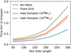 |
Fig. A.1 Compute time for lightcones from z = 35 to z = 6 at various box sizes using two threads and a 2 Mpc cell size. Blue: Previous source model of 21cmFAST (see ‘v3 Default’ runs in Section 6 Orange: Runs with a non-stochastic source field (see ‘CHMF on grid’ in section 6). Green: runtime for the halo sampler using a minimum mass of 108 M⊙. Red: Runtime for the halo sampler using a minimum mass of 1010. The new filters described in section 4 and the halo sampler at 108 M⊙ each add approximately 50% to the runtime, compared with the gridbased model. |
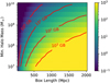 |
Fig. A.2 Memory usage of the halo sampler versus minimum sampled mass and box side length at redshift z = 6. Contours are drawn at 1, 10, 100 and 1000 GB. Since the halo catalogues are the largest data objects in the simulation, this corresponds to the size of two halo catalogues (required for sampling from a descendant catalogue) at z = 6. |
Appendix B Comparison of sampling methods
To provide further justification of our method of sampling halo masses, we compare results here between our direct samples of the conditional mass function (described in Section 2.2) and two other methods for generating halo populations from a Lagrangian density distribution: the mass partitioning method from Sheth & Lemson (1999), where mass from a condition is allocated to halos according to the collapsed fraction distribution, and the binary merger tree algorithm from Parkinson et al. (2008), which uses small internal time-steps, taking the limit of the conditional mass function as the progenitor redshift approaches the descendant redshift zprog → zdesc . Both of these methods have been used for the efficient generation of halo populations (McQuinn et al. 2007; Benson et al. 2016; Qiu et al. 2021; Trinca et al. 2022), however their applications have so far been to produce single halo populations consistent with a certain N-body simulation, which has been achieved by fitting parameters in each model. The goal of our model is to produce halo populations consistent with any given conditional mass function, and so directly sampling the given CHMF is a more natural choice.
We show the mass functions in Lagrangian mean-density cells between redshifts z = 6 and z = 30 for each halo sampling method in Figure B.1. All models shown utilise the Extended Press-Schechter CHMF, and the initial samples at z = 6 are the same number-limited sampling described in section 2. We show two cases in the figure: the first using the EPS mass function with no corrective factors and the second showing various corrective measures to each method so that the final halo samples are a better match the EPS mass function.
We see in the top panels of Figure B.1 that with no corrective factors, the Sheth & Lemson (1999) partitioning method and our mass-limited sampling perform very similarly, with a slight excess at all progenitor masses which increases toward higher redshift. This excess originates from a lack of strict mass conservation in these models. Since we draw a discrete number of halos from the CHMF, we cannot guarantee that their masses sum to the expected mass above our resolution. Separate testing has shown that this excess is not strongly dependent on the choice of CHMF or the cell density, δ. This effect is partially mitigated in the mass-limited sampling case by utilising a strategy which has the opposite bias. Half of the time, once the mass limit is reached, we keep or throw away the final sampled halo depending on which decision brings us closer to the expected total mass. The other half of the time, we remove random halos from our sample until we are below the mass limit again, and then as before we keep the final halo selected for removal if it brings us closer to the expected mass. The result of this process is a ∼1% excess in mass per time-step, which does not strongly depend on the halo mass, the condition, or the chosen CHMF. The binary split algorithm on the other hand shows a defecit of halo mass compared to the EPS mass function, which increases both toward higher redshift and higher halo mass, consistent with the investigation performed in Cole et al. (2008).
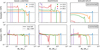 |
Fig. B.1 Mass functions of mean density δ = 0 Lagrangian cells utilising three different sampling methods. Left: Mass-limited sampling described in section 2 Middle: Mass partitioning method described in Sheth & Lemson (1999). Right: Binary merger tree algorithm detailed in Parkinson et al. (2008). Top: Application of an unmodified EPS mass function in each case. Bottom: Adjustments made to the samplers (detailed in the text) to better match the expected EPS mass function. |
In the bottom panels of Figure B.1 we demonstrate the effects of various corrective measures on these methods. For the masslimited sampling we simply multiply the mass threshold for each halo by 0.9, which should be reflected as a downward shift in the HMF. For the partitioning algorithm we multiply each sampled peak  by 0.9, representing a leftward shift in the HMF. For the binary split algorithm we scale the EPS mass function by factors dependent on the condition mass and collapse threshold (Parkinson et al. 2008),
 (B.1)
(B.1)
where we use G0 = 1.0 γ1 = 0.2 γ2 = −0.3. We see that in each case the sampled mass functions are much closer to the expected EPS mass function.
Since each sampling method is comparable in terms of speed, we make the decision to use the mass-limited sampling for this work as it is much more flexible for a general CHMF. The mass partitioning method gains a lot of its speed from the fast sampling of the Gaussian EPS mass distribution. A more general CHMF slows the algorithm down due to the extra sampling steps required per halo sample, and it is not as amenable to tabulation of the CHMF since the condition changes throughout each sample, requiring an extra dimension in the tables.
It would be possible to fit the scaling factors in the binary split algorithm to any given CHMF, as has been done for N -body simulations (Benson et al. 2016; Qiu et al. 2021), and these scaling factors are provided as free parameters should a user wish to perform this analysis. However, since our mass limited sampler performs similarly in both speed and accuracy with the same corrective factor for both EPS and SMT conditional mass functions, we adopt this as our fiducial sampling method throughout this work.
Appendix C Statistics of the halo fields and comparison with N-body
In Section 2, we verify that our halo sampling method produces results consistent with the assumed halo mass functions, both at the cell level and across the simulated volume. In this appendix, we examine the statistics of our sampler in more detail, comparing our samples to halo catalogues from an N -body + hydro code.
In Figure C.1 we present three different 1- and 2-point statistics at z = 8 (left to right): (i) the halo power spectrum; (ii) the mean halo mass function; and (iii) the standard deviation of the halo mass function, normalised by the mean (also known as the coefficient of variation, CV). For (i) we include halos down to 109 M⊙. For (ii) and (iii) we compute the mean and standard deviation over (2 cMpc)3 Eulerian volumes, showing the statistics across the entire volume as solid lines, and showing subsets of the volume at overdensities δ ≈ −0.5, 0, 1 as dashed, dot-dashed, and dotted lines, respectively.
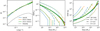 |
Fig. C.1 One- and two-point statistics of 21cmFASTv4 and an N -body + hydro code at z = 8. We show results from our direct number-limited halo sampling (green lines) and correlated mass-limited halos sampling starting at z = 5.5 (orange lines). We also show statistics from ASTRID Friends-of-Friends catalogues (blue lines). Panels from left to right show the halo power spectrum, the mean HMF within 2Mpc Eulerian (evolved) cells, and the standard deviation divided by mean σ/µ (CV) of the HMF averaged over the same cells as in the middle panel. HMF statistics are presented as solid lines for all cells, dashed lines for δ ∈ (−0.6, −0.4), dot-dashed lines for δ ∈ (−0.1, 0.1), and dotted lines for δ ∈ (0.9, 1.1). |
In each panel, the orange and green curves correspond to our fiducial (300 Mpc)3 simulation. The orange curves correspond to halo catalogues produced from the correlated sampling method outlined in section 2 beginning from z = 5.5, whereas the green curves correspond to direct samples of the CHMF at z = 8, using the initial number-limited sampling method on the linear density grid. The blue curves on the other hand correspond to the (250 h−1Mpc)3 ASTRID simulation (Bird et al. 2022)23. In all statistics, the direct and correlated 21cmFAST samples produce consistent results. This is expected since neither the power spectrum nor the HMF statistics are affected by temporal correlations. However, the fact that the number-limited and mass-limited sampling methods produce similar variance serves to further validate the self-consistency of our model.
The halo power spectrum and the HMF statistics computed on the entire volume are consistent with ASTRID. The conditional HMF statistics also show good agreement at low halo masses and average to high overdensities. However, the differences can reach a factor of two lower CV in voids and for the most rare, biased halos.
It is difficult to pin-point the origin of such differences without a detailed comparison that matches the assumed cosmology, initial conditions, analytic HMF used in our sampler, as well as the choice of halo finding algorithm used in the N-body. Indeed, there are non-negligible differences at the field level just between different N-body solvers and halo finding algorithms, even when matched to the same cosmology and initial conditions (e.g. Gómez et al. 2022; Bayer et al. 2025). The fact that we have achieved a decent agreement in global one- and two-point statistics in an out of the box comparison is encouraging. We leave further exploration to future work.
References
- Abdurashidova, Z., Aguirre, J. E., Alexander, P., et al. 2022, ApJ, 924, 51 [NASA ADS] [CrossRef] [Google Scholar]
- Alsing, J., Wandelt, B., & Feeney, S. 2018, MNRAS, 477, 2874 [NASA ADS] [CrossRef] [Google Scholar]
- Alvarez, M. A., & Abel, T. 2012, ApJ, 747, 126 [Google Scholar]
- Barkana, R., & Loeb, A. 2004, ApJ, 609, 474 [NASA ADS] [CrossRef] [Google Scholar]
- Bayer, A. E., Villaescusa-Navarro, F., Sharief, S., et al. 2025, arXiv e-prints [arXiv:2505.13620] [Google Scholar]
- Becker, G. D., D’Aloisio, A., Christenson, H. M., et al. 2021, MNRAS, 508, 1853 [NASA ADS] [CrossRef] [Google Scholar]
- Behroozi, P., Wechsler, R. H., Hearin, A. P., & Conroy, C. 2019, MNRAS, 488, 3143 [NASA ADS] [CrossRef] [Google Scholar]
- Benson, A. J., Cannella, C., & Cole, S. 2016, Computat. Astrophys. Cosmol., 3, 3 [Google Scholar]
- Bernal, J. L., & Kovetz, E. D. 2022, A&A Rev., 30, 5 [NASA ADS] [CrossRef] [Google Scholar]
- Bird, S., Ni, Y., Di Matteo, T., et al. 2022, MNRAS, 512, 3703 [NASA ADS] [CrossRef] [Google Scholar]
- Bond, J. R., Cole, S., Efstathiou, G., & Kaiser, N. 1991, ApJ, 379, 440 [NASA ADS] [CrossRef] [Google Scholar]
- Breitman, D., Mesinger, A., Murray, S. G., et al. 2024, MNRAS, 527, 9833 [Google Scholar]
- Brorby, M., Kaaret, P., Prestwich, A., & Mirabel, I. F. 2016, MNRAS, 457, 4081 [NASA ADS] [CrossRef] [Google Scholar]
- Choudhury, T. R., & Paranjape, A. 2018, MNRAS, 481, 3821 [NASA ADS] [CrossRef] [Google Scholar]
- Choudhury, T. R., Paranjape, A., & Bosman, S. E. I. 2021, MNRAS, 501, 5782 [Google Scholar]
- Cole, S., Lacey, C. G., Baugh, C. M., & Frenk, C. S. 2000, MNRAS, 319, 168 [Google Scholar]
- Cole, S., Helly, J., Frenk, C. S., & Parkinson, H. 2008, MNRAS, 383, 546 [Google Scholar]
- Croton, D. J., Stevens, A. R. H., Tonini, C., et al. 2016, ApJS, 222, 22 [Google Scholar]
- Curti, M., Mannucci, F., Cresci, G., & Maiolino, R. 2020, MNRAS, 491, 944 [Google Scholar]
- Curti, M., Maiolino, R., Curtis-Lake, E., et al. 2024, A&A, 684, A75 [NASA ADS] [CrossRef] [EDP Sciences] [Google Scholar]
- Das, A., Mesinger, A., Pallottini, A., Ferrara, A., & Wise, J. H. 2017, MNRAS, 469, 1166 [NASA ADS] [CrossRef] [Google Scholar]
- Davies, F. B., & Furlanetto, S. R. 2022, MNRAS, 514, 1302 [NASA ADS] [CrossRef] [Google Scholar]
- Davies, J. E., Bird, S., Mutch, S., et al. 2023, MNRAS, 525, 2553 [NASA ADS] [CrossRef] [Google Scholar]
- De Looze, I., Cormier, D., Lebouteiller, V., et al. 2014, A&A, 568, A62 [NASA ADS] [CrossRef] [EDP Sciences] [Google Scholar]
- D’Odorico, V., Bañados, E., Becker, G. D., et al. 2023, MNRAS, 523, 1399 [CrossRef] [Google Scholar]
- Fragos, T., Lehmer, B. D., Naoz, S., Zezas, A., & Basu-Zych, A. 2013, ApJ, 776, L31 [CrossRef] [Google Scholar]
- Furlanetto, S. R., Zaldarriaga, M., & Hernquist, L. 2004, ApJ, 613, 1 [NASA ADS] [CrossRef] [Google Scholar]
- Furlanetto, S. R., Oh, S. P., & Briggs, F. H. 2006, Phys. Rep., 433, 181 [Google Scholar]
- Gagnon-Hartman, S., Davies, J. E., & Mesinger, A. 2025, A&A, 699, A131 [NASA ADS] [CrossRef] [EDP Sciences] [Google Scholar]
- Geda, R., Goulding, A. D., Lehmer, B. D., Greene, J. E., & Kulkarni, A. 2024, ApJ, 965, 67 [NASA ADS] [CrossRef] [Google Scholar]
- Gelli, V., Mason, C., & Hayward, C. C. 2024, ApJ, 975, 192 [NASA ADS] [CrossRef] [Google Scholar]
- Ghara, R. 2023, GRIZZLY: 1D radiative transfer code, Astrophysics Source Code Library [record ascl:2310.012] [Google Scholar]
- Ghara, R., Mellema, G., Giri, S. K., et al. 2018, MNRAS, 476, 1741 [NASA ADS] [CrossRef] [Google Scholar]
- Gómez, J. S., Padilla, N. D., Helly, J. C., et al. 2022, MNRAS, 510, 5500 [CrossRef] [Google Scholar]
- Greig, B., & Mesinger, A. 2015, MNRAS, 449, 4246 [NASA ADS] [CrossRef] [Google Scholar]
- Harikane, Y., Ouchi, M., Oguri, M., et al. 2023, ApJS, 265, 5 [NASA ADS] [CrossRef] [Google Scholar]
- Hassan, S., Davé, R., McQuinn, M., et al. 2022, ApJ, 931, 62 [NASA ADS] [CrossRef] [Google Scholar]
- Hutter, A. 2018, MNRAS, 477, 1549 [Google Scholar]
- Hutter, A., Dayal, P., Yepes, G., et al. 2021, MNRAS, 503, 3698 [NASA ADS] [CrossRef] [Google Scholar]
- Iliev, I. T., Mellema, G., Ahn, K., et al. 2014, MNRAS, 439, 725 [Google Scholar]
- Jasche, J., & Wandelt, B. D. 2013, MNRAS, 432, 894 [Google Scholar]
- Jenkins, A., Frenk, C. S., White, S. D. M., et al. 2001, MNRAS, 321, 372 [Google Scholar]
- Kaur, H. D., Gillet, N., & Mesinger, A. 2020, MNRAS, 495, 2354 [NASA ADS] [CrossRef] [Google Scholar]
- Kaur, H. D., Qin, Y., Mesinger, A., et al. 2022, MNRAS, 513, 5097 [NASA ADS] [CrossRef] [Google Scholar]
- Kreilgaard, K. C., Mason, C. A., Cullen, F., Begley, R., & McLure, R. J. 2024, A&A, 692, A57 [NASA ADS] [CrossRef] [EDP Sciences] [Google Scholar]
- Lacey, C., & Cole, S. 1993, MNRAS, 262, 627 [NASA ADS] [CrossRef] [Google Scholar]
- Lehmer, B. D., Eufrasio, R. T., Basu-Zych, A., et al. 2021, ApJ, 907, 17 [NASA ADS] [CrossRef] [Google Scholar]
- Lovell, C. C., Starkenburg, T., Ho, M., et al. 2024, MNRAS, submitted [arXiv:2411.13960] [Google Scholar]
- Lu, T.-Y., Mason, C. A., Mesinger, A., et al. 2025, A&A, 697, A69 [NASA ADS] [CrossRef] [EDP Sciences] [Google Scholar]
- Mas-Ribas, L., Sun, G., Chang, T.-C., Gonzalez, M. O., & Mebane, R. H. 2023, ApJ, 950, 39 [Google Scholar]
- Mason, C. A., Trenti, M., & Treu, T. 2023, MNRAS, 521, 497 [NASA ADS] [CrossRef] [Google Scholar]
- McQuinn, M., Lidz, A., Zahn, O., et al. 2007, MNRAS, 377, 1043 [Google Scholar]
- Meriot, R., & Semelin, B. 2024, A&A, 683, A24 [NASA ADS] [CrossRef] [EDP Sciences] [Google Scholar]
- Mesinger, A. 2019, The Cosmic 21-cm Revolution; Charting the first billion years of our universe [Google Scholar]
- Mesinger, A., & Furlanetto, S. 2007, ApJ, 669, 663 [Google Scholar]
- Mesinger, A., Furlanetto, S., & Cen, R. 2011, MNRAS, 411, 955 [Google Scholar]
- Mirocha, J., Furlanetto, S. R., & Sun, G. 2017, MNRAS, 464, 1365 [NASA ADS] [CrossRef] [Google Scholar]
- Monaco, P., Theuns, T., & Taffoni, G. 2002, MNRAS, 331, 587 [Google Scholar]
- Muñoz, J. B., Qin, Y., Mesinger, A., et al. 2022, MNRAS, 511, 3657 [CrossRef] [Google Scholar]
- Mutch, S. J., Geil, P. M., Poole, G. B., et al. 2016, MNRAS, 462, 250 [NASA ADS] [CrossRef] [Google Scholar]
- Mutch, S. J., Greig, B., Qin, Y., Poole, G. B., & Wyithe, J. S. B. 2024, MNRAS, 527, 7924 [Google Scholar]
- Nasirudin, A., Iliev, I. T., & Ahn, K. 2020, MNRAS, 494, 3294 [NASA ADS] [CrossRef] [Google Scholar]
- Ni, Y., Genel, S., Anglés-Alcázar, D., et al. 2023, ApJ, 959, 136 [NASA ADS] [CrossRef] [Google Scholar]
- Nikolic´, I., Mesinger, A., Qin, Y., & Gorce, A. 2023, MNRAS, 526, 3170 [CrossRef] [Google Scholar]
- Nikolic´, I., Mesinger, A., Davies, J. E., & Prelogovic´, D. 2024, A&A, 692, A142 [NASA ADS] [CrossRef] [EDP Sciences] [Google Scholar]
- Nikolic´, I., Mesinger, A., Mason, C. A., et al. 2025, A&A, 699, A323 [Google Scholar]
- Pallottini, A., & Ferrara, A. 2023, A&A, 677, L4 [NASA ADS] [CrossRef] [EDP Sciences] [Google Scholar]
- Pallottini, A., Ferrara, A., Gallerani, S., et al. 2022, MNRAS, 513, 5621 [NASA ADS] [Google Scholar]
- Park, J., Mesinger, A., Greig, B., & Gillet, N. 2019, MNRAS, 484, 933 [NASA ADS] [CrossRef] [Google Scholar]
- Parkinson, H., Cole, S., & Helly, J. 2008, MNRAS, 383, 557 [Google Scholar]
- Prelogovic´, D., & Mesinger, A. 2023, MNRAS, 524, 4239 [CrossRef] [Google Scholar]
- Qin, Y., Mesinger, A., Park, J., Greig, B., & Muñoz, J. B. 2020, MNRAS, 495, 123 [Google Scholar]
- Qin, Y., Mesinger, A., Bosman, S. E. I., & Viel, M. 2021a, MNRAS, 506, 2390 [NASA ADS] [CrossRef] [Google Scholar]
- Qin, Y., Mesinger, A., Greig, B., & Park, J. 2021b, MNRAS, 501, 4748 [Google Scholar]
- Qin, Y., Mesinger, A., Prelogovic´, D., et al. 2025, PASA, 42, e049 [Google Scholar]
- Qiu, Y., Mutch, S. J., Elahi, P. J., et al. 2021, MNRAS, 500, 493 [Google Scholar]
- Ren, K., Trenti, M., & Mason, C. A. 2019, ApJ, 878, 114 [Google Scholar]
- Rubiño-Martín, J. A., Betancort-Rijo, J., & Patiri, S. G. 2008, MNRAS, 386, 2181 [CrossRef] [Google Scholar]
- Satyavolu, S., Kulkarni, G., Keating, L. C., & Haehnelt, M. G. 2024, MNRAS, 533, 676 [Google Scholar]
- Savchenko, O., Abellán, G. F., List, F., Anau Montel, N., & Weniger, C. 2025, arXiv e-prints [arXiv:2502.03139] [Google Scholar]
- Saxena, A., Cole, A., Gazagnes, S., et al. 2023, MNRAS, 525, 6097 [NASA ADS] [CrossRef] [Google Scholar]
- Schaeffer, T., Giri, S. K., & Schneider, A. 2023, MNRAS, 526, 2942 [NASA ADS] [CrossRef] [Google Scholar]
- Scoccimarro, R. 1998, MNRAS, 299, 1097 [NASA ADS] [CrossRef] [Google Scholar]
- Shen, X., Vogelsberger, M., Boylan-Kolchin, M., Tacchella, S., & Kannan, R. 2023, MNRAS, 525, 3254 [NASA ADS] [CrossRef] [Google Scholar]
- Sheth, R. K., & Lemson, G. 1999, MNRAS, 305, 946 [Google Scholar]
- Sheth, R. K., & Tormen, G. 2002, MNRAS, 329, 61 [Google Scholar]
- Sheth, R. K., Mo, H. J., & Tormen, G. 2001, MNRAS, 323, 1 [NASA ADS] [CrossRef] [Google Scholar]
- Sobacchi, E., & Mesinger, A. 2013, MNRAS, 432, L51 [NASA ADS] [CrossRef] [Google Scholar]
- Sobacchi, E., & Mesinger, A. 2014, MNRAS, 440, 1662 [NASA ADS] [CrossRef] [Google Scholar]
- Songaila, A., & Cowie, L. L. 2010, ApJ, 721, 1448 [NASA ADS] [CrossRef] [Google Scholar]
- Tinker, J., Kravtsov, A. V., Klypin, A., et al. 2008, ApJ, 688, 709 [Google Scholar]
- Trac, H., Chen, N., Holst, I., Alvarez, M. A., & Cen, R. 2022, ApJ, 927, 186 [NASA ADS] [CrossRef] [Google Scholar]
- Tramonte, D., Rubiño-Martín, J. A., Betancort-Rijo, J., & Dalla Vecchia, C. 2017, MNRAS, 467, 3424 [NASA ADS] [CrossRef] [Google Scholar]
- Trapp, A. C., & Furlanetto, S. R. 2020, MNRAS, 499, 2401 [CrossRef] [Google Scholar]
- Trinca, A., Schneider, R., Valiante, R., et al. 2022, MNRAS, 511, 616 [NASA ADS] [CrossRef] [Google Scholar]
- Vale, A., & Ostriker, J. P. 2006, MNRAS, 371, 1173 [NASA ADS] [CrossRef] [Google Scholar]
- Visbal, E., Barkana, R., Fialkov, A., Tseliakhovich, D., & Hirata, C. M. 2012, Nature, 487, 70 [NASA ADS] [CrossRef] [Google Scholar]
- Yeh, J. Y. C., Smith, A., Kannan, R., et al. 2023, MNRAS, 520, 2757 [NASA ADS] [CrossRef] [Google Scholar]
- Zahn, O., Mesinger, A., McQuinn, M., et al. 2011, MNRAS, 414, 727 [NASA ADS] [CrossRef] [Google Scholar]
- Zhao, X., Mao, Y., & Wandelt, B. D. 2022, ApJ, 933, 236 [NASA ADS] [CrossRef] [Google Scholar]
Throughout this work ‘Lagrangian’ refers to the initial conditions, computed here at z = 300, whereas ‘Eulerian’ refers to the gravitationally-evolved matter field at lower redshifts. Analytic HMF frameworks typically operate on the Lagrangian field, connecting this linear field to non-linear structures using spherical or ellipsoidal collapse models.
Since we sample the CHMF independently to produce this initial halo population, it follows that we should use the Poisson distribution to characterise the total number of halos within the cell. However, there is no guarantee that this assumption is correct (e.g. samples from neighbouring cells could be correlated beyond just through the mean overdensities used in the CHMFs). In Appendix C, we demonstrate that our halo fields are in decent agreement with results from N-body simulations using both one- and two-point statistics.
This value is specific to the SMT mass function. Generally speaking, it is the condition for halo formation at the descendant redshift (possibly dependent on halo mass, redshift or other factors), evolved to the progenitor redshift.
While it may seem reasonable to enforce a more strict level of mass conservation within each descendant, in practice this skews the resulting mass functions, as certain samples are more likely to fall within a given mass tolerance. Progenitor samples are not directly correlated with one another, so we would see a large deficit of halos around Mprog = Mdesc/2 since samples including halos at this mass are far less likely to meet any mass tolerance criteria.
To be more precise, relations such as the SHMR and the SFMS typically refer to the running averages of these conditional distributions, obtained by fitting a line in log-log space. Here, we sample from the full conditional probability densities, which include also scatter around the mean relations.
A multi-tracer approach is especially important during the EoR/CD, as existing data-sets are very complementary: direct galaxy observations with Hubble/JWST provide information about rare, bright galaxies while IGM and LIM observations are sensitive to the cumulative photon emission that is dominated by the abundant, faint galaxies far below detection limits of JWST (e.g. Breitman et al. 2024; Qin et al. 2021b).
As discussed in the previous section, our algorithm steps backwards in time and therefore the progenitor properties are sampled after those of the descendant.
The X-ray and Lyman band optical depth calculation remains unchanged from previous versions of 21cmFAST. Specifically, the Lyman band optical depth assumes a picket fence absorption at each Lyman transition, while we assume a step function opacity for X-rays at the frequency corresponding to an optical depth of unity (an approximation verified to be accurate in Das et al. (2017). See Mesinger et al. (2011) for more details.
The numerical (trapezoidal) integration of equation 20 forces us to use a finite ∆R ≡ Ro - Ri, We confirm that if we use the infinitely thin spherical shell limit window function (i.e. ∆R → 0), we obtain noticeable aliasing and miss small scale emissivity fluctuations.
We make the standard assumption that helium is singly ionised together with hydrogen.
The EoR history is insensitive to this choice when accounting for inhomogeneous sub-grid recombinations (e.g. Qin et al. 2025). This is because the total mean free path during the majority of the EoR λtot is dominated by the typical distance to HI patches, λEoR, with  (e.g. Alvarez & Abel 2012). Indeed, recent measurements (Becker et al. 2021) suggest a much shorter mean-free path <10 c Mpc for ionising photons at z ~ 6, which could be due in part to the contribution of residual HI patches and/or details in how it is computed from observations (Satyavolu et al. 2024; Qin et al. 2025).
This model is analogous to the source models labelled FFRT-P in Davies & Furlanetto (2022) or ESF-E in Trac et al. (2022).
Because we assume log-normal scatter, the only difference between these models is a factor of  in each scaling relation, where the ‘normalised’ scaling relations represent a mean μx, as opposed to the median (or equivalently the exponent of the mean logarithm 10μiogx) of the galaxy property (see Section 3). These conditional probability distributions need not be log-normal, in which case the normalisation to obtain a fixed global mean emissivity could be computed numerically.
Specifically, we use particle and Friends-of-Friends data from ASTRID-ES (Davies et al. 2023), a re-run of ASTRID to z = 5.5 with an on-the-fly excursion-set reionisation model. The dark matter and halo properties of this simulation are identical to ASTRID
All Tables
Settings of the simulations performed to investigate the effect of stochasticity in halo masses and bulk galaxy properties.
All Figures
|
Fig. 1 Example usage case for 21cmFASTv4. First, cosmological parameters are sampled, and an associated realisation of the Lagrangian matter field is generated. Dark matter halos are identified in Lagrangian space and then moved, together with the matter field, to Eulerian space using 2LPT. This is shown in the left-middle panel as a slice through a 300 Mpc overdensity field at z = 7, with the 300 largest halos in the 2 Mpc-thick slice shown as red circles. Then galaxies are assigned to DM halos by sampling parametric conditional probability densities based on well-established empirical relations such as the SHMR, SFMS, FMR, etc. Cosmic radiation fields (Lyman-alpha, Lyman-continuum, and X-ray) sourced by these galaxies are calculated using approximate radiative transfer, and the IGM is evolved accordingly. The lower panel shows slices corresponding to the IGM neutral fraction, 21cm brightness temperature, and CII surface brightness density, at the same redshift as the overdensity field and with the same halos overlaid as red circles. We can then extract statistics of these fields for comparison with multi-tracer observations. In the centre-right panel we show the ultraviolet (UV) luminosity function at z = 7, the 21cm power spectrum at the midpoint of reionisation, the evolution of the 21cm power spectrum at k = 0.1 Mpc−1, and the CII x 21cm cross-power spectrum at z = 12. Under fiducial settings, 21cmFASTv4 computes all of these steps in ≲3 core hours for a single realisation, thus facilitating high-dimensional, multi-tracer, field-level Bayesian inference of cosmology and astrophysics during the EoR and CD. |
| In the text | |
|
Fig. 2 Top: conditional halo mass functions from our sampler at z = 10 (solid black line) and the Sheth-Tormen CHMF (Equation (3), shown as a blue dotted line) in 10 000 under-dense (left, δ = −0.9) mean density (middle, δ = 0.0) and over-dense (right, δ = 1.4) Lagrangian cells of volume (2 Mpc)3 . Their ratio is indicated on the right vertical axis and shown as a solid red line which follows the target of unity (red dotted lines). Bottom: distribution of the number of halos (red curve) and total mass of halos (black curve) within each cell. The average of the distribution and the expected average from the Sheth–Tormen CHMF are shown as solid and dotted vertical lines, respectively. The agreement between the mean computed from samples and the target mean is evidenced by the overlapping solid and dotted lines. |
| In the text | |
|
Fig. 3 Same as Figure 2, but sampling from 10000 descendant halos of mass 109, 1010, and 1011 M⊙ from redshift zdesc = 6 to the progenitor redshift, zprog = (1 + zdesc)∆z - 1, where ∆z = 1.02. Samples drawn from descendant halos use the mass-limited sampling described above, rather than the number-limited sampling used for the cells. The short time step results in a very tight distribution of total progenitor mass, although the number of halos and their mass distribution can vary significantly between individual descendants. |
| In the text | |
|
Fig. 4 Correlated sampling of halos from z = 6 to z = 30 within a 300 cMpc box. Top: total halo mass function within the box at from redshifts z = 6 to z = 30, compared to the Sheth-Tormen unconditional mass function represented as a shaded region with Poisson uncertainty. The black dotted line corresponds to a number density of one halo in the simulation volume within that bin. Bottom: ratio of the sampled mass function to the expected Sheth–Tormen unconditional mass function, showing an excess of small halos at the highest redshifts, but remaining within Poisson errors over the vast majority of masses and redshifts. |
| In the text | |
|
Fig. 5 Distributions of stellar to halo mass (top) and star formation rate to stellar mass (bottom) at z = (6.0,7.7,12). Orange and blue points correspond to galaxies taken from two hydrodynamical simulations: the zoom-in simulation suite SERRA (Pallottini et al. 2022) and the large cosmological simulation Astrid (Bird et al. 2022). For the SERRA sample we plot every central galaxy at these redshifts, while for Astrid we plot a subsample randomly selected in fixed logarithmic mass bins. Both codes have been calibrated to reproduce observable data at Mh ≳ 1012M⊙, but predict very different SHMRs for the unseen, faint galaxies that dominate the EoR and CD. The orange and blue contours correspond to two different parameter combinations in 21cmFASTv4 whose conditional distributions can characterise the correspondingly-coloured galaxy populations from the different hydro codes. These contours correspond to 2-5 σ of the joint distributions, P(M*, Mh) and P(SFR, M*), highlighting how the vast majority of galaxies are expected to be far below the resolution limits for large-scale cosmological simulations. This figure demonstrates that our semi-empirical model is flexible, capable of capturing a large range of predictions, and eventually allowing us to infer such galaxy properties from multi-tracer galaxy and IGM observations. |
| In the text | |
|
Fig. 6 Galaxy properties within 323 Lagrangian cells with side length 2 Mpc at exactly mean density (δcond = 0), including stochastically sampled halos above 108 M⊙ showing the variance in galaxy properties solely from the sampling of halo populations and galaxy properties. We show halo mass density (top), cumulative ionising photon density per hydrogen atom (middle) and X-ray soft-band emissivity (bottom). Solid and dotted black lines show the mean and median of the distribution respectively, and green lines show the expected mean obtained by integrating the CHMF. Blue shaded regions span the [2.5, 97.5] percentile range, and the thin red lines show 32 randomly selected individual cells. Changes over time in the summed galaxy properties are caused by the growth of halos, as well as the variability in the stellar to halo mass ratio and specific star formation rate. |
| In the text | |
|
Fig. 7 Co-location of galaxies and the 21cm brightness temperature fields in our illustrative simulation during key stages in the history of the CD and EoR. We show slices at z = 14.8, z = 9.0, and z = 7.0, corresponding to epochs of Lyman alpha coupling, X-ray heating, and reionisation, respectively. Green circles denote 200 galaxies with the brightest UV magnitudes in each slice, with larger circles corresponding to brighter galaxies. |
| In the text | |
|
Fig. 8 21cm brightness temperature lightcones from four runs of 21cmFAST. From left to right: ‘v3 Default’ shows the previous default model, where the source field is calculated on the filtered density grids, ‘CHMF on Grid’ shows a model where there is a one-to-one relationship between cell density and emissivities, based on the integral of the CHMF; ‘v4 No Astro Scatter’ shows the effects of our halo sampler described in Section 2, without any stochasticity in the galaxy properties. We show two cases for the model with stochasticity in the halo mass distribution and galaxy properties, which differ in their interpretations of the scaling relations; ‘v4 Mean Norm’ shows the case where the scaling relations are defined by the mean of each property’ and ‘v4 No Norm’ shows the case where the scaling relations are defined by the mean logarithm. In the latter case, increasing the log-normal scatter also increases the mean emissivities at all wavelengths. |
| In the text | |
|
Fig. 9 21cm power spectra shown for the same five models as in Figure 8. We show the power-spectra at two points in cosmic history: the midway point of the EoR (the snapshot at which the total ionised fraction is closest to 50%), as well during X-ray heating where the volume-weighted mean brightness temperature |
| In the text | |
|
Fig. 10 21cm brightness temperature power spectra from 21cmFASTv4 runs with differing levels of astrophysical scatter. The top rows show the runs where the scaling relations have a fixed (linear) mean as scatter increases, whereas the bottom rows show runs where the mean is allowed to increase with the scatter (i.e. at a fixed log-log mean relation). The left column shows the epoch during X-ray heating where |
| In the text | |
|
Fig. 11 UV luminosity functions at z = 8 by setting the scatter in the galaxy properties to either zero (blue line), equal to the fiducial values from Table 1 (orange line), and increased by factors of 2 (green line) or 3 (red line). Top: runs where the scaling relations are normalised to have the same linear mean. Bottom: runs where log-normal scatter is simply added to a fixed log-log mean relation. In both cases increasing scatter results in a flattening of the relation; however, in the later case it also results in significantly brighter galaxies overall. |
| In the text | |
|
Fig. 12 Lightcones containing example outputs from 21cmFASTv4 with default parameters. The leftmost panel shows the evolved matter density field. The next two panels show gridded galaxy properties: cumulative ionising photon density per hydrogen atom and soft-band X-ray emissivity. The two rightmost panels show observables: the 21cm brightness temperature and CII surface brightness density. |
| In the text | |
|
Fig. 13 Schematic showing how different galaxy populations affect IGM and LIM observables. Top: SHMR panels from Figure 5, where we set our galaxy scaling relations to be consistent with either the SERRA or Astrid cosmological simulations. Middle: resulting 21cm brightness temperature and CII surface brightness density lightcones in the range 6 < z < 16. Bottom: auto power spectra from both fields, as well as their cross power spectrum at the midpoint of reionisation |
| In the text | |
|
Fig. A.1 Compute time for lightcones from z = 35 to z = 6 at various box sizes using two threads and a 2 Mpc cell size. Blue: Previous source model of 21cmFAST (see ‘v3 Default’ runs in Section 6 Orange: Runs with a non-stochastic source field (see ‘CHMF on grid’ in section 6). Green: runtime for the halo sampler using a minimum mass of 108 M⊙. Red: Runtime for the halo sampler using a minimum mass of 1010. The new filters described in section 4 and the halo sampler at 108 M⊙ each add approximately 50% to the runtime, compared with the gridbased model. |
| In the text | |
|
Fig. A.2 Memory usage of the halo sampler versus minimum sampled mass and box side length at redshift z = 6. Contours are drawn at 1, 10, 100 and 1000 GB. Since the halo catalogues are the largest data objects in the simulation, this corresponds to the size of two halo catalogues (required for sampling from a descendant catalogue) at z = 6. |
| In the text | |
|
Fig. B.1 Mass functions of mean density δ = 0 Lagrangian cells utilising three different sampling methods. Left: Mass-limited sampling described in section 2 Middle: Mass partitioning method described in Sheth & Lemson (1999). Right: Binary merger tree algorithm detailed in Parkinson et al. (2008). Top: Application of an unmodified EPS mass function in each case. Bottom: Adjustments made to the samplers (detailed in the text) to better match the expected EPS mass function. |
| In the text | |
|
Fig. C.1 One- and two-point statistics of 21cmFASTv4 and an N -body + hydro code at z = 8. We show results from our direct number-limited halo sampling (green lines) and correlated mass-limited halos sampling starting at z = 5.5 (orange lines). We also show statistics from ASTRID Friends-of-Friends catalogues (blue lines). Panels from left to right show the halo power spectrum, the mean HMF within 2Mpc Eulerian (evolved) cells, and the standard deviation divided by mean σ/µ (CV) of the HMF averaged over the same cells as in the middle panel. HMF statistics are presented as solid lines for all cells, dashed lines for δ ∈ (−0.6, −0.4), dot-dashed lines for δ ∈ (−0.1, 0.1), and dotted lines for δ ∈ (0.9, 1.1). |
| In the text | |
Current usage metrics show cumulative count of Article Views (full-text article views including HTML views, PDF and ePub downloads, according to the available data) and Abstracts Views on Vision4Press platform.
Data correspond to usage on the plateform after 2015. The current usage metrics is available 48-96 hours after online publication and is updated daily on week days.
Initial download of the metrics may take a while.