| Issue |
A&A
Volume 701, September 2025
|
|
|---|---|---|
| Article Number | A254 | |
| Number of page(s) | 16 | |
| Section | Planets, planetary systems, and small bodies | |
| DOI | https://doi.org/10.1051/0004-6361/202556015 | |
| Published online | 22 September 2025 | |
Is ozone a reliable proxy for molecular oxygen?
III. The impact of CH4 on the O2–O3 relationship for Earth-like atmospheres
1
Instituto de Astrofísica de Andalucía – CSIC,
Glorieta de la Astronomía s/n,
18008
Granada,
Spain
2
National Space Institute, Technical University of Denmark,
Elektrovej,
2800 Kgs.
Lyngby,
Denmark
3
School of Physics and Astronomy, University of Southampton,
Highfield,
Southampton
SO17 1BJ,
UK
4
School of Ocean and Earth Science, University of Southampton,
Southampton
SO14 3ZH,
UK
★ Corresponding author.
Received:
18
June
2025
Accepted:
7
August
2025
Abstract
In the search for life in the Universe, molecular oxygen (O2) combined with a reducing species, such as methane (CH4), is considered a promising disequilibrium biosignature. In cases where it would be difficult or impossible to detect O2 (such as in the mid-IR or low O2 levels), it has been suggested that ozone (O3), the photochemical product of O2, could be used as a proxy for determining the abundance of O2. As the O2–O3 relationship is known to be nonlinear, the goal of this series of papers is to explore how it would change for different host stars and atmospheric compositions and learning how to use O3 to infer O2. We used photochemistry and climate modeling to further explore the O2–O3 relationship by modeling Earth-like planets with the present atmospheric level (PAL) of O2 between 0.01% and 150%, along with high and low CH4 abundances of 1000% and 10% PAL, respectively. Methane is of interest not only because it is a biosignature, but it is also the source of hydrogen atoms for hydrogen oxide (HOx), which destroys O3 through catalytic cycles, and acts as a catalyst for the smog mechanism of O3 formation in the lower atmosphere. We find that varying CH4 causes changes to the O2–O3 relationship in ways that are highly dependent on both the host star and O2 abundance. A striking result for high CH4 models in high O2 atmospheres around hotter hosts is that enough CH4 is efficiently converted into H2O to significantly impact stratospheric temperatures, and therefore the formation and destruction rates of O3. Changes in HOx have also been shown to influence both the HOx catalytic cycle and production of smog O3, causing variations in harmful UV reaching the surface, as well as changes in the 9.6 μm O3 feature in emission spectra. This study further demonstrates the need to explore the O2–O3 relationship in different atmospheric compositions in order to use O3 as a reliable proxy for O2 in future observations.
Key words: astrobiology / planets and satellites: atmospheres / planets and satellites: terrestrial planets
© The Authors 2025
 Open Access article, published by EDP Sciences, under the terms of the Creative Commons Attribution License (https://creativecommons.org/licenses/by/4.0), which permits unrestricted use, distribution, and reproduction in any medium, provided the original work is properly cited.
This article is published in open access under the Subscribe to Open model. This email address is being protected from spambots. You need JavaScript enabled to view it. to support open access publication.
1 Introduction
Although ozone (O3) is not directly created by life, it is still included in discussions about the search for life in the Universe using atmospheric biosignatures. This is because O3 is the photochemical product of molecular oxygen (O2), which is primarily produced biologically on modern Earth. However, there are multiple scenarios where O2 could build up in a planetary atmosphere in the absence of life, so O2 on its own is not a reliable sign of life (e.g., Hu et al. 2012; Wordsworth & Pierrehumbert 2014; Domagal-Goldman et al. 2014; Tian et al. 2014; Luger & Barnes 2015; Gao et al. 2015; Harman et al. 2015). Instead, O2 and a reducing species such as methane (CH4) is thought to be a promising disequilibrium biosignature, as it would require strong surface fluxes of each species, which would be indicative of surface life (e.g., Lovelock 1965; Lederberg 1965; Lippincott et al. 1967).
Ozone enters the conversation because there are scenarios in which O2 would be difficult or impossible to detect, whereas O3 would be accessible. For a terrestrial planet with low levels of O2 (such as on early Earth), it would be difficult to make an O2 detection, while O3 is detectable at trace amounts (Kasting et al. 1985; Léger et al. 1993). In addition, while the mid-IR (3-20 μm holds many opportunities for biosignature searches (Quanz et al. 2022), there are no significant O2 features, only a collisionally induced absorption feature that is not strong enough for detections of biologically produced O2 (Fauchez et al. 2020). Therefore, many have suggested using O3 as a proxy for O2 in such situations (e.g., Léger et al. 1993; Des Marais et al. 2002; Segura et al. 2003; Léger et al. 2011; Meadows et al. 2018b; Schwieterman et al. 2018).
As O2 and O3 are known to have a highly nonlinear relationship (Ratner & Walker 1972; Kasting & Donahue 1980; Kasting et al. 1985; Segura et al. 2003; Gregory et al. 2021; Kozakis et al. 2022; Kozakis et al. 2025), the goal of this series of papers is to explore the O2–O3 relationship for a variety of host stars and Earth-like atmospheres in order to gain valuable insight on how to use future observations of O3 to predict O2 atmospheric content and potentially identify biosignatures. Here we use the term “Earth-like” to mean a planet with the same planetary parameters as Earth (e.g., radius, gravity), roughly the same atmospheric composition, and an orbital distance from its host star such that it receives the same total amount of flux as on modern Earth. Already we have found that not only is the O2–O3 relationship nonlinear, but that it varies significantly depending on the host star and planetary atmospheric composition. In Kozakis et al. (2022) we modeled planets around a variety of host stars with O2 mixing ratios of 0.01–150% our present atmospheric level (PAL), and in Kozakis et al. (2025) we repeated those same models but with variations of high and low amounts of nitrous oxide (N2O). With both studies we found that trends in the O2–O3 relationship differ from hotter stars to cooler stars, with the pressure-dependent nature of O3 formation playing a large role.
In this study, we focus on the impact of CH4 on the O2–O3 relationship and explore how it could impact future observations of O3. We chose CH4 not only because it is considered a biosignature (e.g., Thompson et al. 2022), but because it is the source of hydrogen oxides (HOx) that power catalytic cycles that destroy O3, as well as processes that create O3 in the lower atmosphere. Section 2 introduces the relevant atmospheric chemistry, Sect. 3 our methodology, and Sect. 4 our results, including changes in atmospheric chemistry, UV to the ground, and O3 emission spectra features. In Sect. 5, we discuss the implications of our results, and Sect. 6 provides our main conclusions.
2 Relevant chemistry
2.1 Ozone formation and destruction
The majority of O3 in the atmosphere of modern Earth is formed in the stratosphere via the Chapman mechanism (Chapman 1930), beginning with O2 photolysis,
 (1)
(1)
 (2)
(2)
which creates either a ground state O atom, or an excited O(1D) radical depending on the energy of the photon. An O(1D) radical can either be quenched back to the ground state with the help of a background molecule, M,
 (3)
(3)
or react with other species. Oxygen atoms can then combine with O2 to create O3,
 (4)
(4)
Reaction (4) requires a background molecule to carry away excess energy, meaning that it is a three-body reaction that favors higher pressures. This reaction in particular additionally favors cooler temperatures. Once O3 has been created, it can be photolyzed to produce O2 and either ground state O atoms or O(1D) radicals,
 (5)
(5)
 (6)
(6)
However, photolysis is not considered a real “loss” of O3, as the O atom and O2 molecule created by O3 photolysis often recombine back into O3 (Reaction (4)). Because O3 and O cycle back and forth through photolysis and recombination with O2, it is useful to keep track of “O + O3”, called “odd oxygen.” A true loss of O3 occurs when odd oxygen is converted into O2,
 (7)
(7)
as O2 photolysis is the limiting reaction of the Chapman mechanism. However, Reaction (7) is not fast, so odd oxygen tends to be destroyed by other methods.
While the Chapman mechanism is the dominant O3 formation mechanism in the stratosphere, “smog formation” (Haagen-Smit 1952) can create O3 in the lower atmosphere,
 (8)
(8)
 (9)
(9)
 (10)
(10)
 (11)
(11)
 (4)
(4)
The smog mechanism requires both nitrogen oxides (NOx, NO3+NO2+NO) and hydrogen oxides (HOx, HO2+OH+H) as catalysts to form O3; neither are consumed in the process.
A true loss of odd oxygen/O3 most typically occurs from catalytic cycles, which take the form,

with the primary catalytic cycles on Earth being that of the NOx (X=NO) and HOx (X=OH) catalytic cycles. The main NOx catalytic cycle is,
 (12)
(12)
 (13)
(13)
with a secondary NOx catalytic cycle working in the lower stratosphere using NO3,
 (12)
(12)
 (14)
(14)
 (15)
(15)
The primary mechanism for removing NOx from the atmosphere is by conversion into stable reservoir species,
 (16)
(16)
 (17)
(17)
 (18)
(18)
2.2 Methane and HOx catalytic cycles
Along with the NOx catalytic cycle the other dominant destruction of O3 is via the HOx catalytic cycle. While H2O is the direct source of HOx in the atmosphere, H2O has limited upward transport due to the cold trap, which prevents travel from the troposphere into the stratosphere, hence the significantly drier stratosphere than the troposphere on modern Earth. However, CH4 can freely move from the ground into the stratosphere, where it can be oxidized into H2O molecules. As a result, CH4 is the primary source of stratosphere HOx, and thus powers the HOx catalytic cycle.
Another popular biosignature, CH4, is produced on Earth primarily from natural wetlands, although it has strong anthropogenic sources such as rice paddies and other agricultural processes that are not addressed in this study. When a molecule of CH4 is transported into the stratosphere, it has the potential to create two H2O molecules given enough oxygen and incoming UV flux. To start off this process, CH4 is oxidized by the hydroxyl radical (OH), to create H2O and the methyl radical CH3,
 (19)
(19)
 (20)
(20)
 (21)
(21)
with the net result of two H2O molecules. Although there is technically a loss of HOx (through OH), the resulting formyl radical (HCO) is frequently converted back into HOx via reactions with O2,
 (22)
(22)
The original source of the OH in Reaction (19) is often via O(1D) reacting with H2O,
 (23)
(23)
Since O(1D) is created by photolysis with high energy UV photons, production is highly dependent on the spectrum of the host star, which we explore in depth in the rest of this study.
Although on modern day Earth the biggest sink of the shortlived OH radical is CH4, OH is also the main sink of CH4 in the atmosphere. Additionally OH is commonly created by O(1D) resulting from O3 photolysis, making O3 an indirect source of HOx. This creates interesting feedback behavior, as HOx is a significant sink of O3 via the HOx catalytic cycle,
 (24)
(24)
 (25)
(25)
in which odd oxygen, O + O3, is converted into two O2 molecules. In the upper stratosphere, where Η atoms are more common (often from H2O photolysis), odd oxygen can be converted to O2 via,
 (26)
(26)
 (25)
(25)
 (27)
(27)
In the lower stratosphere where there is less O2 photolysis and therefore fewer Ο atoms, odd oxygen is destroyed via,
 (28)
(28)
 (29)
(29)
There are multiple reactions that destroy either OH or HO2, but they are typically recycled back into another HOx species. Photolysis is also not a true sink of HOx since HO2 photolysis creates OH, and OH is too short-lived for significant photolysis. Efficient methods of HOx destruction are conversion to H2O,
 (30)
(30)
since the conversion of H2O into HOx is a limiting reaction. HOx is also lost via conversion to a stable reservoir species,
 (31)
(31)
 (17)
(17)
 (18)
(18)
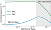 |
Fig. 1 Relationship between NOx and HOx in the lower atmosphere on modern Earth, adapted from Logan et al. (1981). In the NOx-limited regime (white background) an increase of NOx will lead to an increase of HOx and thus increased productivity of the smog mechanism. In the ΝΟx-saturated regime (gray background) the NOx/HOx ratio reaches a tipping point where NOx begins to deplete HOx by locking it up into stable reservoir species, therefore suppressing smog formation. |
2.3 Relationship between NOx and HOx
As mentioned previously, O3 is often an indirect source of HOx as O(1D) radicals that react with H2O to form HOx (Reaction (23)) are typically formed via O3 photolysis (Reaction (5)) in O2-rich atmospheres. This causes an interesting relationship with the smog mechanism of O3 production (Reactions (4), (8), (9), (10), (11)), as both HOx and NOx are required as catalysts. Earth-based studies have found that the amount of NOx present in a region can either increase the rate of smog produced O3 (and thus indirectly increasing HOx) or suppress O3 production by locking HOx up into reservoir species such as HNO3 (Reaction (17)) or HO2NO2 (Reaction (18)). We refer to these two scenarios in which NOx can assist smog production or hinder it as the “NOx-limited” and “NOx-saturated” regimes, respectively, as illustrated in Fig. 1. In the NOx-limited regime, increasing NOx leads to more O3 and therefore more HOx, encouraging smog formation, and in the NOx-saturated regime, the NOx/HOx ratio has become high enough that NOx locks up HOx in reservoir species and suppresses smog formation.
However, it is important to note that these regimes have been studied primarily in the context of NOx pollution on modern Earth via anthropogenic activities, where the emphasis is placed on how changes in NOx (not changes in HOx) impact smog O3 formation. This study provides a new perspective on these ΝΟx regimes, as we focus on changes in HOx caused by varying CH4 levels. These regimes were discussed in depth in Kozakis et al. (2025) where we varied N2O (and therefore NOx) and we found that even for modern levels of N2O and O2 the NOx abundances were already high enough to be in the NOx-saturated regime for planets around all hosts explored in this paper except for the M5V at modern O2 levels, causing severe suppression of the smog mechanism.
3 Methods
3.1 Atmospheric models
We used Atmos1, a publicly available 1D coupled photochemistry and climate code to model the atmospheres of Earth-like planets, following Kozakis et al. (2022) and Kozakis et al. (2025). We briefly describe the code and our chosen parameters here, and refer the reader to other sources for a full description (Arney et al. 2016; Meadows et al. 2018a; Kozakis et al. 2022). Inputs to Atmos require a stellar host spectrum (121.6–45 450 nm), planetary parameters (e.g., radius, gravity), and the initial composition of the atmosphere and boundary conditions.
For the photochemistry code (Kasting 1979; Zahnle et al. 2006) we used the modern Earth template available with Atmos, including 50 gaseous species and 233 chemical reactions. The atmosphere is broken up into 200 plane parallel layers from the planetary surface to 100 km, with the flux and continuity equations solved simultaneously in each individual layer. Vertical transport is included for long-lived species, as well as molecular and eddy diffusion. Radiative transfer is calculated using a δ−2-stream method (Toon et al. 1989), and the code is considered to be converged when the length of the adaptive time step reaches the age of the universe within the first 100 steps.
The climate code (Kasting & Ackerman 1986; Kopparapu et al. 2013; Arney et al. 2016) then uses the atmospheric composition calculated in the photochemistry code along with the incoming stellar flux to calculate temperature and pressure profiles for the atmosphere. Here the atmosphere is broken up into 100 layers from the surface up until 1 mbar (typically <60–70 km), as the code does not run reliably at lower pressures (Arney et al. 2016). When transferring information back to the photochemistry code pressures above 1 mbar hold the temperature constant. Each layer uses a δ−2-stream multiple scattering method to calculate stellar flux absorption. A correlated-k method is used for outgoing IR for O3, H2O, CH4, CO2, and C2H6 with single and multiple scattering. Convergence is reached when the temperature and flux differences out of the top of the atmosphere are considered small enough (~<10–5) (Arney et al. 2016).
For this study we iterated the photochemistry and climate codes back and forth 30 times and utilized the short-stepping technique for better climate code convergence (Teal et al. 2022; Kozakis et al. 2022). Our planets had the same radius and gravity as Earth, and orbited their host stars at the Earth-equivalent distance where they received the same total amount of flux as modern Earth. Fixed mixing ratio abundances of O2 were varied from 0.01% to 150% PAL while additionally varying CH4 (see Table 1). We considered fixed CH4 mixing ratios of 10% and 1000% PAL for high and low CH4 scenarios (same as N2O in Kozakis et al. 2025) to continue exploring the parameter space of possible Earth-like atmospheres and the resulting impact on the O2–Ο3 relationship. We note that for our high CH4 models that the CH4/CO2 ratio is not high enough for haze formation (Arney et al. 2016), and it is therefore not considered in this study. Other relevant gaseous species held at constant mixing ratios of their present atmospheric levels are N2O (3.0 × 10⁻⁶), H2 (5.3 × 10⁻⁷), and CO (1.1 × 10⁻⁷).
Model parameters.
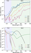 |
Fig. 2 Stellar spectra for the host stars following Kozakis et al. (2022) (top) along with the cross-sections used by Atmos of relevant species (bottom). The ratio of far-UV (FUV) to near-UV (NUV) flux is important in driving atmospheric chemistry, and is indicated by the colored backgrounds. The abrupt cutoff of NO2, N2O, and HO2 cross-sections is due to the extremely low photolysis rates of those species at shorter wavelengths due to absorption from other atmospheric species (i.e.. CO2). |
3.2 Input stellar spectra
For host stars we used the same stellar spectra as in Kozakis et al. (2022) and Kozakis et al. (2025), shown in Fig. 2 along with absorption cross-sections of relevant species. For the G0V-K5V hosts the UV data came from International Ultraviolet Explorer (IUE) data archives2 combined with synthetic ATLAS data for visible and IR wavelengths (Kurucz 1979). Our M5V host is GJ 876 from the Measurements of the Ultraviolet Spectral Characteristics of Low-mass Exoplanetary Systems (MUSCLES) survey (France et al. 2016). For full details of all host star spectra, see Rugheimer et al. (2013) and Kozakis et al. (2022).
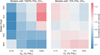 |
Fig. 3 Ozone abundances normalized to the amount produced at modern levels of CH4 for both the high (left) and low (right) CH4 models for all host stars at 0.1%, 1%, 10%, and 100% PAL O2. The most striking result is that for the high CH4 models there is less O3 compared to modern CH4, except for planets around the hottest hosts at 100% PAL O2. This is due both to the indirect impact of CH4 on the stratospheric temperature, as well as a boost in the smog mechanism due to a decreased NOx/HOx ratio. The rest of the cases for the CH4 models show increased O3 depletion due to a higher amount of CH4 from the increased efficiency of the HOx catalytic cycle’s ability to destroy O3. |
3.3 Post-processing radiative transfer models
To explore the observational impacts of the changing O2–O3 relationship, we used the Planetary Intensity Code for Atmospheric Scattering Observations (PICASO) to simulate planetary emission spectra, using model atmosphere results from Atmos following Kozakis et al. (2022). PICASO3 (Batalha et al. 2019, 2021) is a publicly available code capable of simulating transmission, reflectance, and emission spectra, using atmospheric composition and temperature/pressure profiles calculated by atmospheric modeling codes. We simulated our model planets at full phase (0°) from 0.3 to 14 μm, and focused in particular on the 9.6 μm O3 feature. We note that although it is unlikely for a planet to be imaged at full phase, it should not have a significant impact on mid-IR for a planet with minimal day-to-day temperature contrast.
4 Results
We found that the impact of CH4 on the O2–O3 relationship cannot be generalized, as it changes depending on the host star and the amount of O2. In Sect. 4.1 we explored the impact on atmospheric chemistry, changes in UV to the ground in Sect. 4.2, and impact on simulated planetary emission spectra in Sect. 4.3. Supplementary figures and tables are available in Appendix A.
4.1 Atmospheric chemistry
4.1.1 Atmospheric chemistry: Overview
Overall planet models were affected more by the high CH4 models than the low CH4 models, with higher CH4 either depleting or increasing the total O3 abundance compared to atmospheres with modern levels of CH4 depending on the host star and O2 level, as seen in Figs. 3 and 4. The greatest increase in O3 from different CH4 levels was experienced by the Sun-hosted planet with the high CH4 model at 100% O2 PAL, resulting in 122% of the original O3 abundance. The most O3 depletion also occurred with the high CH4 models but for the K2V-hosted planet at 0.1% PAL O2 where it retains only 62% of the original O3 abundance.
An initially striking result is that for the high CH4 models planets around all host stars at all O2 levels display O3 depletion when compared to models with modern levels of CH4, except for those around the hottest host stars (G0V-K2V) at O2 levels similar to modern Earth. The increased O3 for the high CH4 models around hotter hosts (as well as the decreased O3 for the corresponding cases with the low CH4 models) might seem counterintuitive as CH4 is the parent molecule for HOx, which catalytically destroys O3 (Sect. 2.2). Indeed, HOx species are consistently more abundant with all high CH4 models, powering more efficient HOx catalytic cycles that destroy O3. The main processes affecting the O2–O3 relationship when varying CH4 abundance are:
the amount of stratospheric H2O and HOx created by CH4,
indirect effects of CH4 on stratospheric temperature,
smog mechanism efficiency as NOx/HOx ratio changes,
changing HOx/O3 ratio at different O2 levels.
We go into detail on each of these processes in the following subsections.
4.1.2 Atmospheric chemistry: Efficiency of converting CH4 to HOx
As summarized in Sect. 2.2, a CH4 molecule can be converted into two H2O molecules (Reactions (19), (20), (21)) given enough UV light and oxygen to power this process. In particular, OH, which begins this reaction chain, is formed by the O(1D) radical reacting with H2O (Reaction (23)), which is created via photolysis,
 (2)
(2)
 (5)
(5)
 (32)
(32)
 (33)
(33)
allowing planets with high amounts of incoming UV flux to be more efficient at converting CH4 into H2O. In addition, the main source of O(1D) radicals is typically from O3 photolysis (as it can be photolyzed at longer wavelengths than the other options), which causes the conversion of CH4 into H2O to favor oxygen-rich environments. Due to the UV and oxygen requirements, conversion rates of CH4 into H2O and then into HOx are faster for planets around hosts with higher UV flux at higher O2 levels.
The higher levels of HOx that the high CH4 models bring cause faster HOx catalytic cycles that destroy O3. However, planets around the 3 hottest hosts at 100% PAL O2 experience an increase in O3 for the high CH4 models, despite the fact that they are the hosts converting the most CH4 into HOx. The reason behind this O3 increase is due to the indirect impact of CH4 on stratospheric temperature, and the efficiency of the smog mechanism for planets around those hosts with high amounts of HOx.
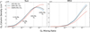 |
Fig. 4 Absolute values of the O2–O3 relationship at all O2 and CH4 levels modeled for planets around the Sun (left) and M5V (right) hosts. O2 levels of 0.1%, 1%, 10%, and 100% PAL are marked with vertical dashed lines to enable easier comparison with Fig. 3. This figure highlights the stark difference in how CH4 impacts the O2–O3 relationship differently for hotter and cooler host stars, due primarily to the amount of UV flux arriving at the planet. For hotter hosts the higher UV flux allows more efficient conversion of CH4 into H2O and then HOx compared to the lower UV flux of M5V host. Full O2–O3 relationships of all hosts including comparisons to Kozakis et al. (2025) are located in Appendix A. |
4.1.3 Atmospheric chemistry: Indirect impact of CH4 on stratospheric temperature
Planets around hotter hosts at high O2 levels are the most efficient at converting CH4 into HOx, but also into H2O. Although this increases the amount of H2O converted into HOx, another effect of the large amount of stratospheric H2O is that it forms at a high enough altitude to have a cooling effect. Unlike in the troposphere, where H2O heats the atmosphere as a greenhouse gas, in the stratosphere H2O radiates heat into space, similar to CO2 stratospheric cooling seen on modern Earth (Goessling & Bathiany 2016; Santer et al. 2023). In the stratosphere, H2O radiates more in the infrared than absorbs energy coming from the lower atmosphere, resulting in a net cooling. This causes atmospheres with enough excess H2O to experience significant stratospheric cooling, especially for planets with hotter hosts at high O2 as shown in Fig. 5. For the low CH4 cases the opposite occurs where there is less stratospheric H2O, causing a warmer stratosphere when compared to modern levels of CH4, although the effect is smaller than for the high CH4 cases.
Stratospheric cooling caused by excess H2O for the hottest hosts at high O2 causes two main changes in the O3 abundance:
a faster Chapman mechanism and faster O3 production,
a slower NOx catalytic cycle and slower O3 destruction.
Stratospheric cooling from increased H2O abundance occurs for a range of O2 levels for the planets around the G0V and Sun hosts, but only to the extent that it overcomes the depletion of O3 from the faster HOx catalytic cycles at high O3 with high CH4.
4.1.4 Atmospheric chemistry: Smog mechanism efficiency with changing HOx
In addition to the faster O3 production and slower O3 destruction due to stratospheric cooling from excess H2O with the high CH4 models, planets hosted by the hottest stars also experience a boost in O3 production from the smog mechanism. Although HOx is not directly created or consumed by the smog mechanism (Reactions (4), (8), (9), (10), (11)), it is necessary to the process as a catalyst. As discussed in both Sects. 2.1 and 2.3, at high enough levels of NOx the atmosphere will enter the NOx-saturated regime and NOx will begin to deplete HOx by converting it into reservoir species (see Fig. 1). Planets around hotter stars (G0V-K2V) in particular have enough NOx in their lower stratospheres to place them in the NOx-saturated regime for modern levels of N2O, resulting in significant HOx depletion.
In Kozakis et al. (2025) we determined which NOx regime an atmosphere was in by looking at the NOx abundance, but in this study we took a different approach because it is HOx, not NOx, that has significant variation. In environments where there are greatly increased levels of HOx, we find that the cutoff of NOx that determines the NOx-saturated and NOx-limited regimes changes. It is seen in Fig. 6 for the planet around the Sun at 100% PAL O2 with the high CH4 models that there is a significant decrease in depletion of HO2 caused by high ΝΟx when compared to models with modern levels of CH4. Although the planet around the Sun at modern levels of O2 and NOx was squarely in the NOx-saturated regime, since the NOx/HOx ratio is smaller with the increased CH4 there is significantly less HO2 depletion indicating that the atmosphere has been pushed toward the NOx-limited regime. We see evidence of this occurring for the G0V, Sun, and K2V hosts at O2 levels near 100% PAL O2 with the high CH4 models, resulting in a boost of smog mechanism-produced O3. This is the other part of the puzzle as to why planets around these hosts experience an increase in O3 with the high CH4 models at modern O2 levels.
The smog mechanism is also the reason that the M5V-hosted planet with the high CH4 models experiences less O3 depletion as O2 levels decrease, as opposed to planets around all other hosts which experience more O3 depletion with decreasing O2. The planet around the M5V host is the only one to always exist in the NOx-limited regime, and therefore does not suffer from suppression of the smog mechanism as do planets around the other hosts. In addition, smog formation becomes even more efficient at lower O2 levels as HOx is “pushed” closer to the ground as UV shielding from O2 and O3 decreases. Photolysis allows HOx to form deeper in the atmosphere, allowing the lower atmosphere HOx to speed up smog formation even further (see Kozakis et al. 2022 for a longer discussion of this process). This effect occurs for planets around all host stars, but unlike planets around other hosts, for the M5V-hosted planet the extra O3 produced from the smog mechanism has a more significant impact on the O2–Ο3 relationship since smog-produced O3 makes up a much larger portion of the total O3 abundance. This is because the Chapman mechanism has a photon requirement of less than 242 nm for O2 photolysis, whereas the smog mechanism can be fulfilled with near-UV and visible photons for the required NO2 photolysis (see Figure 2). The low UV flux of the M5V host allows the smog mechanism to take on a larger role in O3 production than for planets around hotter hosts. For this reason for the high CH4 models with the M5V-hosted planet the amount of O3 depletion decreases with decreasing O2. As the amount of Chapman-produced O3 from O2 photolysis decreases, increased amounts of smog-produced O3 from added HOx are more significant.
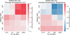 |
Fig. 5 Average stratospheric H2O (left) and temperatures (right) for high CH4 models all normalized to results from models using modern levels of CH4. Nearly all models experience an increase in H2O for the high CH4 models due to the conversion of CH4 into H2O in the stratosphere. Planets around hotter hosts with higher O2 show the largest increases as incident UV and O2 are necessary for creating H2O in this scenario. The excess H2O impacts the temperature, providing stratospheric cooling in cases with large increases of H2O. As the atmosphere is thin in the stratosphere heat radiating from H2O can escape to space, causing an effect similar to stratospheric CO2 cooling present on modern Earth. |
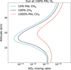 |
Fig. 6 Profiles of HO2 for the planet around the Sun at 100% PAL O2 and different levels of CH4. The significant HO2 depletion present for low and modern levels of CH4 is lessened for the high CH4 models. This is because the HO2 depletion is due to the Sun-hosted planet being in the NOx-saturated regime, but increased CH4 allows enough HOx production to lessen this effect. |
4.1.5 Atmospheric chemistry: Changing HOx/O3 ratio
For planets around all hosts other than the M5V as the O2 level decreases, a larger portion of O3 is depleted. This is because as O2 abundance decreases, the HOx/O3 ratio increases. As discussed in Sect. 4.1.2, conversion from CH4 into HOx is more efficient at higher O2 levels as O3 is often an indirect source of HOx. Formation of HOx occurs when H2O reacts with O(1D) radicals, which are most easily formed from O3 photolysis when there is sufficient O3 supply, as O3 can be photolyzed by much longer wavelength photons than the other suppliers of O(1D): O2, N2O, and CO2 (Reactions (2), (5), (32), (33)). However, when O3 (and O2) levels decrease, HOx begins to source O(1D) radicals more from photolysis of N2O and CO2. Although this requires higher energy photons, it is also easier for these species to be photolyzed deeper into the atmosphere as O2 and O3 levels decrease (causing less UV shielding), thus creating a larger HOx/O3 ratio with decreasing O2. With a higher HOx/O3 ratio the HOx catalytic cycle has an easier time depleting O3 at these lower O2 levels. As discussed in the previous section (Sect. 4.1.4) this effect of increasing amounts of O3 depletion occurring at lower O2 levels does not occur for the M5V-hosted planet due to the boost in smog-produced O3.
4.2 UV to ground
Variations in O3 caused by different CH4 abundances resulted in varying amounts of UV shielding in the atmosphere, and therefore different amounts of UV flux reaching the surface of our model planets. The level of potential biological damage that UV photons can inflict is dependent on wavelength, described by three UV regimes that we used here. UVA (315–400 nm) is the lowest energy UV and least dangerous, and is not shielded by O3; UVB (280–315 nm) is responsible for skin tanning and skin cancer, and is partially shielded by O3; and lastly UVC (121.6–280 nm) is capable of significant biological harm, but is fortunately well shielded by O3 and O2, assuming that they exist in significant quantities in the atmosphere. Along with being the most dangerous, UVC surface flux also has a highly nonlinear relationship with the amount of O3 in the atmosphere, as it is UVC flux (<242 nm; Reactions (1), (2)) that is necessary for the Chapman mechanism to produce O3. Results for UVC surface flux variations at 100%, 10%, 1%, and 0.1% PAL O2 are shown in Fig. 7, along with a table for UVB and UVC results in the Appendix (Table A.1). As in Kozakis et al. (2022) UVA surface flux did not vary with changing O2 or CH4 values (always ~80% reaching the surface) so it is not discussed here.
As UVB flux is partially shielded by O3, varying CH4 causes changes to the amount of UVB photons reaching the ground in some cases, but only very slightly. The largest decrease was for the Sun-hosted planet at 100% PAL O2 with the high CH4 models having only 80% of the original UVB surface flux due to increased O3 shielding. The largest increase in UVB surface flux was also at 100% PAL O2 for the high CH4 models, but this time with the M5V-hosted planet receiving 124% the UVB surface flux that it did with modern levels of CH4. For O2 levels under 100% PAL changes in the amount of UVB flux arriving at the surface changed only slightly, with larger effects being seen consistently with the high CH4 models due to the larger impact on O3 formation and destruction (see Table A.1).
Changes in UVC surface flux were much more significant, due to the larger absorption cross-sections at these wavelengths. The highest increases and decreases of UVC surface flux corresponded to the same models with the largest UVB surface flux differences: the planets around the Sun and M5V hosts, both for the high CH4 models at 100% PAL O2. The planet around the Sun experienced a factor of just 7.5 × 10⁻⁵ times the original UVC flux at modern levels of CH4 due to the increased amounts of O3 caused by stratospheric cooling, decreased NOx catalytic cycle efficiency, and extra smog production. The largest increase in UVC surface flux from the planet around the M5V host (receiving a factor of 2.1×10⁴ more) was due to the increased ability for the HOx catalytic cycle to destroy O3. For the low CH4 models the largest variations in UVC surface flux were similarly at 100% PAL O2 with the largest increase in surface UVC for the planet around the Sun with a factor of 22 times more UVC surface flux, and the largest decrease was for the M5V-hosted planet having 5.8 × 10⁻² times the original UVC flux due to the decreased ability of the HOx catalytic cycle to destroy O3. For lower oxygen levels the variation in O3 was significantly decreased, causing the variation in UVC surface flux to be minimized, with the amount of UVC flux variation compared to modern CH4 levels not exceeding an order of magnitude.
4.3 Planetary emission spectra
We additionally generated planetary emission spectra to explore the potential impact on future observations that varying CH4 could have on the 9.6 μm O3 feature. Emission spectral features are highly influenced by the temperature difference between the emitting and absorbing layers of the atmosphere, which as shown in Kozakis et al. (2022) is particularly relevant when considering O3 features. Since O3 NUV absorption is the primary source of stratospheric heating on modern Earth, there is a counterintuitive effect where a planet with large amounts of O3 can have a shallower emission feature than a planet with significantly less O3. This is because a planet experiencing stratospheric heating via O3 will have a decreased temperature difference between the planetary surface and stratosphere, resulting in a shallower emission spectral feature depth. However, this will only happen for planets receiving sufficient NUV flux from their host, as this is required for said stratospheric heating to occur. This is shown in the left panel of Fig. 8, where variations in the 9.6 μm O3 feature from just varying O2 in Kozakis et al. (2022) are shown. For a more detailed discussion of this phenomena, see Kozakis et al. (2022).
Once again it the high CH4 models had more of an impact than the low CH4 models (see Fig. 8). Planets around hotter hosts experienced the most variability in the O3 feature due to different CH4 and O2 abundances, owing to the indirect impact of CH4 on stratospheric temperature. For planets that experienced stratospheric cooling from high H2O content, O3 spectral features are much deeper both because of increased O3 abundance, but also from the larger temperature difference between the emitting and absorbing layers of the atmosphere. However, at lower O2 levels for planets around these same hosts the O3 features became shallower than with modern CH4 abundances, due to lower O3 abundances from the higher destruction rates of O3 via more productive HOx catalytic cycles. For all other cases the high CH4 models resulted in shallower O3 spectral features, again due to the decreased amounts of O3 from the higher efficiency of the HOx catalytic cycle. Stratospheric temperatures did not vary significantly in these cases, leading to changes in the O3 feature depth corresponding more directly to changes in O3 abundance. It is also worth noting that atmospheres with the high CH4 models had generally hotter surface temperatures and atmospheres as CH4 is a greenhouse gas. Overall feature depth changed the most for planets around the G0V and Sun hosts with the high CH4 models, as they experienced significant deepening of features at high O2 levels, and much shallower features at low O2 levels.
5 Discussion
5.1 Comparison to impact of N2O on the O2–O3 relationship
This paper is in many ways a “sister study” to Kozakis et al. (2025), which varied N2O instead of CH4 in order to understand how it would impact the O2–O3 relationship. Both N2O and CH4 are potential biosignatures (Schwieterman et al. 2018; Schwieterman et al. 2022; Thompson et al. 2022; Angerhausen et al. 2024), power the primary catalytic cycles (with NOx and HOx), and influence the smog mechanism of O3 formation. However, we found that Earth-like atmospheres experience different responses to variations and N2O and CH4, depending on both the amount of O2. As the ultimate goal of this paper series is to explore and navigate the challenges of using O3 as a proxy for O2, it is useful to compare how N2O and CH4 impact the O2–O3 relationship differently. Figures comparing results from Kozakis et al. (2025) and this study are located in Appendix A.
Overall at higher O2 levels (> ~ 1% PAL O2) varying N2O had a stronger impact on the total amount of O3 for planets around all stars except for the M5V host, due to changing efficiency of the NOx catalytic cycle (Fig. A.1). For the high N2O models at high O2 the depletion of O3 was the most extreme, causing orders of magnitude differences in harmful UVC flux reaching the ground – significantly larger changes than when varying CH4 (Fig. A.3 and Table A.1). For lower O2 levels high CH4 led to O3 depletion, while high N2O resulted in increased O3 formation from a boost to the smog mechanism. Changes in the O3 abundance at these lower O2 levels from the low N2O and CH4 models were much smaller. Both N2O and CH4 were found to impact the smog mechanism, demonstrating in different scenarios the importance of the NOx/HOx ratio in determining if smog production would be enhanced or suppressed. However, it was only variations in CH4 that induced atmospheric changes that could significantly alter atmospheric temperature profiles (through production or lack of production of stratospheric H2O).
Looking at the 9.6 μm O3 feature from the simulated emission spectra (Fig. A.4), it is clear that planets around every host star were impacted from the variations in either N2O either/or CH4. The cases least affected were around the coolest hosts at the lowest O2 values. The most significant changes overall in the O3 spectral feature were for the K2V-hosted planet at 100% PAL O2 with high N2O, which was ironically the only case that was relatively untouched by CH4 variations at 100% PAL O2. Planets around the G0V and Sun hosts faced the most variations in how N2O and CH4 impacted the O3 feature based on the O2 level, with high N2O causing shallower features at high O2 and deeper features at low O2, with the reverse occurring for the high CH4 models. We also find that the O3 feature of the M5V-hosted planet was only significantly changed by variations in CH4, not in N2O. Planets around all other hosts experienced spectral feature changes from both N2O and CH4 variations to some degree. For future observations it seems that understanding the N2O and CH4 content of a planetary atmosphere will be important if we wish to use O3 as a proxy for O2, although our results thus far indicate that changes in N2O will be less relevant for planets around hosts like the M5V star used here, but that CH4 can have much more of an effect on O3 abundance.
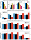 |
Fig. 7 Comparisons of UVC results with modern CH4 abundances (top row) with incident top-of-atmosphere (TOA) UVC flux and surface UVC flux for all hosts with modern levels of CH4 at different O2 levels, and surface UVC flux with varying CH4 for 100% PAL O2 (second row), 10% PAL O2 (third row) and 0.1% PAL O2 (bottom row). Surface UVC plots from Kozakis et al. (2022) use the same y-axis limits as the corresponding plots in the bottom three rows to enable easier comparison. Changes in UVC surface flux are most significant for 100% PAL O2 due to the dependency of oxygen to convert CH4 into H2O and HO2. |
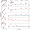 |
Fig. 8 Comparisons of the 9.6 μm O3 emission spectra feature for all hosts at different O2 levels using modern levels of CH4 (left) and O3 features for different CH4 abundances (right) normalized to features with modern levels of CH4. Normalized O3 features use the same y-axis limits for all host stars in order to compare the difference in impact of CH4 on O3 for different hosts. For the hottest hosts at 100% PAL O2 changes in feature strength are due to changes in O3 abundances as well as stratospheric temperatures differences from H2O abundance, while the rest of the model spectra variations are due mainly to changes in O3 due to variations in CH4. |
5.2 Comparisons to other studies
Although this is the first study to vary both O2 and CH4 in Earthlike atmospheres orbiting a variety of host stars with the goal of studying the impact on O3, there are several other studies exploring similar concepts. Grenfell et al. (2006) varies both CH4 and O2 abundances (along with NOx, H2, and CO) in the context of Proterozoic Earth to evaluate the role of smog-produced O3 in UV shielding during that time period. They focus on O2 levels used in this study (10% and 100% PAL O2) but adopt CH4 mixing ratios an order of magnitude larger than we used with our high CH4 models (1.0 × 10⁻⁴ and 3.0 × 10⁻⁴). Therefore we cannot compare directly to our results for the planet around the Sun, but we do see some similar trends. Grenfell et al. (2006) found that NOx was the main driver in changing O3 production, but that when NOx abundances were high enough to enter the NOx-saturated regime, increasing CH4 (and therefore HOx) provided a boost in the smog mechanism. This agrees with our results for the hottest hosts in our study at high O2 (and therefore the highest NOx), as we found that increased CH4 and HOx helped to counteract NOx-saturated atmospheres and increased the amount of smog-produced O3 (see Fig. 6). Despite the different parameter spaces in Grenfell et al. (2006) and this study, both display the same trends of the importance of the NOx/HOx ratio determining the efficiency of the smog mechanism, and that in high NOx environments extra HOx results in more smog-produced O3.
Grenfell et al. (2014) also varies CH4 on an Earth-like planet, but around an M7V host star. They focus on the impact on biosignatures when varying biological surface fluxes of N2O and CH4, along with the UV spectrum of the host star, using CH4 fluxes 100 times less than present day, and 2 and 3 times that of present day. Although they see some similar trends to the work in this study (and results agreeing well with Kozakis et al. 2025) the differences in CH4 boundary conditions (fixed surface flux rather than fixed mixing ratio) and different UV abundances make it difficult to draw many direct comparisons. That being said, there are no direct contradictions to the findings of this study, with differences in results likely due to different parameter space and boundary conditions.
Searching through the literature we could not find any studies replicating our results of stratospheric cooling via excess H2O with our high CH4 models around hotter hosts, although several studies find high amounts of H2O production in high CH4 atmospheres (e.g., Segura et al. 2005; Rauer et al. 2011). We do not believe our results of stratospheric cooling contradict any existing studies as this is the first to model such levels of O2 and CH4 around hotter hosts, and stratospheric cooling due to greenhouse gases such as CO2 has been modeled and observed on modern Earth (e.g., Goessling & Bathiany 2016; Santer et al. 2023).
We also note that the decision to use fixed mixing ratios as the boundary condition for certain species (O2, N2O, CH4, H2, CO) impacts our results differently than if we were to use fixed surface fluxes. As discussed in Kozakis et al. (2022) and Kozakis et al. (2025), species such as N2O and CH4 have been shown to build up in the atmospheres of Earth-like planets around cooler host stars due to the low incident UV flux (e.g., Rugheimer et al. 2015; Wunderlich et al. 2019; Teal et al. 2022). In addition, CO abundance (which is strongly interlinked with CH4 abundance) has been shown to similarly build up in such environments (see Schwieterman et al. 2019 and references therein). We reiterate here that our choice in fixed mixing ratio boundary conditions is to enable easier comparison between the differences in the O2–O3 relationship for planets around different host stars. The impact of different boundary conditions will be explored at length in future work.
5.3 Plausible CH4 mixing ratios in Earth-like atmospheres
The purpose of this study was to further evaluate potential changes in the O2–O3 relationship when CH4 levels are varied, and our choice of using CH4 abundances of 10% and 1000% PAL was motivated by the need to begin filling out the parameter space over which Earth-like exoplanets may exist. The plausible range of CH4 in the atmospheres of such planets is still unknown, but we can use our knowledge of CH4 abundances over the geological history of Earth as a rough guide.
A complication to making such predictions is that surface flux and resulting atmospheric mixing ratios of CH4 are nonlinear (similar to N2O), with a strong dependency on the abundance of O2 and other oxidizing species. O2 combined with CH4 is said to be a promising disequilibrium biosignature pair due to the fact that they react quickly with each other and large surface fluxes of O2 and CH4 are required to allow significant amounts of both to co-exist in an Earth-like atmosphere. The amount of CH4 that is able to accumulate in the atmosphere is additionally dependent on the type of host star, where similarly to N2O, planets around cooler hosts with less incoming UV allow for a larger buildup of CH4 (e.g., Segura et al. 2003; Rugheimer et al. 2013).
On the early Earth before the Great Oxidation Event CH4 was likely significantly higher in abundance due to the reducing atmosphere and lack of appreciable O2, and it is possible that during the Archean era that CH4 abundances could have been greater than 1000 ppm (e.g., Arney et al. 2016; Catling & Zahnle 2020). Thompson et al. (2022) and Akahori et al. (2024) both modeled surface fluxes of CH4 to see the corresponding CH4 atmospheric mixing ratios around the Archean Earth, before the rise of O2, around the Sun and other spectral hosts. They found that during this time period although there was very little O2, CH4 still faced destruction from photolysis and reactions with OH created from H2O photolysis.
After the rise of O2 it is possible that there was still a significant amount of CH4 in the atmosphere, perhaps contributing significantly to the warming of the Proterozoic Earth (Roberson et al. 2011), although it also is possible that there was not significant CH4 during this era (e.g., Olson et al. 2016). The relationship between CH4 surface flux and atmospheric mixing ratios has been explored at length in Gregory et al. (2021), which varied both CH4 and O2 surface fluxes, as they highly impact the stability of both species in the atmosphere. In Kozakis et al. (2025) we were able to discuss an actual limit of biologically produced N2O, but with CH4 there is no known maximum limit of biological CH4 surface flux. As such, it is unknown how much CH4 can accumulate in the atmosphere of an O2-rich planet.
6 Summary and conclusions
This study expands on previous work by considering the impacts of different amounts of atmospheric CH4 on the O2–O3 relationship for an Earth-like planet. We find that the impact of varying CH4 on the O2–O3 relationship is highly influenced by both the host star and the amount of O2 in the atmosphere, in a manner similar to when N2O is varied (Kozakis et al. 2025). Increasing CH4 to 1000% PAL in our high CH4 models was found to have significantly more of an impact on O3 than when we decreased CH4 to 10% PAL with our low CH4 models (Sect. 4.1). The most striking result is that planets around the hottest hosts with high O2 abundances (>50% PAL) experienced the opposite response of O3 to CH4 to all other models we explored. There are two main reasons for this effect. First, in high UV environments for models with plentiful O2 and high CH4 large amounts of stratospheric H2O were created, which resulted in cooler stratospheres that increased O3 production and slowed down its destruction, in a process similar to stratospheric cooling via CO2 on modern Earth. Second, for these hotter hosts at high O2 there was a boost in O3-produced smog with the high CH4 models, as the additional HOx created from H2O resulted in a higher NOx/HOx ratio than with modern levels of CH4. This allowed these “NOx -saturated” atmospheres to have faster smog mechanisms as it was more difficult for NOx to lock up the available HOx into reservoir species. For the hottest hosts at lower O2 levels, as well as all models around cooler hosts, the high CH4 models resulted in lower O3 abundances than compared with modern levels of CH4. This was primarily due to the increased efficiency of the HOx catalytic cycle in destroying O3.
The largest absolute changes in O3 abundance due to variations in CH4 occurred at higher O2 levels, causing the amount of harmful UVC reaching the surface of our model planets to change significantly, especially for the high CH4 models (Sect. 4.2). At 100% PAL O2 for the high CH4 models the planets orbiting the Sun and M5V hosts experienced factors of 7.5 × 10⁻⁵ and 2.1 × 10⁴ times the amount of UVC surface flux, respectively, when compared to models with modern levels of CH4. When considering how this could impact future observations we looked at the 9.6 μm O3 feature in planetary emission spectra (Sect. 4.3). We found again that the high CH4 models had the most impact, with planets around all hosts being affected to some degree depending on the amount of O2 in the atmosphere. Planets orbiting the G0V and Sun hosts with the high CH4 models had the most change in the O3 feature dependent on the O2 level, with the extra CH4 sometimes causing a deeper or shallower feature.
These results further complicate the usage of O3 as a proxy for O2, but also provide additional guidance for future observations. We have now shown in this study that varying CH4 impacts the O2–O3 relationship just as much as N2O (Kozakis et al. 2025), but in different ways. There are many scenarios where high CH4 could be increasing the O3 of an atmosphere, while high N2O would be working at the same time to deplete that O3. This shows that we would be required to think about variations of both species in order to use an O3 measurement to learn about the O2 content of the atmosphere. Once again we gain no general rules about how O3 would be impacted when thinking about variations in CH4 or N2O, with the specific host star playing a highly influential role.
We find that untangling the impact of CH4 and N2O on the O2–O3 relationship might be more straightforward for cooler stars, especially around hosts like the M5V star used in this study as N2O impacts on O3 are minimal, with CH4 mainly impacting the atmosphere at higher O2 abundances. Planets around hotter hosts like our G0V and Sun hosts have the potential to more significantly alter O3 measurements, as impacts from CH4 and N2O on O3 change significantly based on the O2 content of the atmosphere. Careful modeling and retrieval studies exploring the parameter space of O2, N2O, and CH4 for Earth-like atmospheres will be necessary if we wish to glean information about the amount of O3 – and therefore O2 – in a exoplanetary atmosphere when the time comes that we are able to perform such observations.
Acknowledgements
This project is funded by VILLUM FONDEN and all computing was performed on the HPC cluster at the Technical University of Denmark (DTU Computing Center 2021). Authors TK and LML acknowledge financial support from Severo Ochoa grant CEX2021-001131-S funded by MCIN/AEI/10.13039/501100011033. JMM acknowledges support from the Horizon Europe Guarantee Fund, grant EP/Z00330X/1. We thank the anonymous referee for their useful comments, which improved the clarity of our manuscript.
Appendix A Supplementary figures and tables
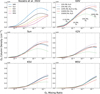 |
Fig. A.1 Relationships of O2–O3 for all host stars at all O2 and CH4 levels modeled, along with comparisons to varying levels of N2O as modeled in Kozakis et al. (2025). All plots share the same y-axis scale to facilitate comparisons. For planets around all hosts except the M5V there are larger variations in O3 when varying N2O rather than CH4. Only the M5V-hosted planet exhibits stronger changes in O3 with CH4 variations. |
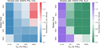 |
Fig. A.2 Abundances of O3 for both high CH4 models from this study and high N2O models from Kozakis et al. (2025) normalized to the amount of O3 with modern amounts of CH4 and N2O for all host stars at 0.1%, 1%, 10%, and 100% PAL O2. Both figures share the same color bar limits in order to facilitate comparisons. |
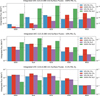 |
Fig. A.3 Comparisons of UVC surface flux for all hosts at 100%, 10% and 0.1% PAL O2, as well as high and low CH4 and N2O variations from this study as well as Kozakis et al. (2025). The dashed horizontal lines indicate the amount of O3 for models with modern levels of both CH4 and N2O. Overall variations in N2O have a stronger impact on UVC surface flux, with larger changes when varying CH4 present primarily at 100% PAL O2. |
UV integrated fluxes
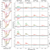 |
Fig. A.4 Comparisons of 9.6 μm O3 emission spectra features from Kozakis et al. (2022) with modern levels of CH4 and N2O (left) and O3 features from varying CH4 and N2O models normalized to modern amounts of CH4 and N2O (right). Y-axis limits for all normalized features are the same to allow for comparison between different O2 levels and host stars. For both variations in CH4 and N2O changes in the O3 feature were primarily due to differences in O3 abundance rather than changes in the atmospheric temperature profiles. The exception being for the CH4 models for the hotter stars at 100% PAL O2, which experienced stratospheric temperature changes depending on the amount of H2O produced from CH4. |
References
- Akahori, A., Watanabe, Y., & Tajika, E. 2024, ApJ, 970, 20 [Google Scholar]
- Angerhausen, D., Pidhorodetska, D., Leung, M., et al. 2024, AJ, 167, 128 [NASA ADS] [CrossRef] [Google Scholar]
- Arney, G., Domagal-Goldman, S. D., Meadows, V. S., et al. 2016, Astrobiology, 16, 873 [Google Scholar]
- Batalha, N. E., Marley, M. S., Lewis, N. K., & Fortney, J. J. 2019, ApJ, 878, 70 [NASA ADS] [CrossRef] [Google Scholar]
- Batalha, N., Rooney, C., & MacDonald, R. 2021, https://doi.org/10.5281/zenodo.5093710 [Google Scholar]
- Catling, D. C., & Zahnle, K. J. 2020, Sci. Adv., 6, eaax1420 [NASA ADS] [CrossRef] [Google Scholar]
- Chapman, S. A. 1930, Mem. R. Met. Soc., 3, 103 [Google Scholar]
- Des Marais, D. J., Harwit, M. O., Jucks, K. W., et al. 2002, Astrobiology, 2, 153 [NASA ADS] [CrossRef] [Google Scholar]
- Domagal-Goldman, S. D., Segura, A., Claire, M. W., Robinson, T. D., & Meadows, V. S. 2014, ApJ, 792, 90 [CrossRef] [Google Scholar]
- DTU Computing Center 2021, DTU Computing Center resources, https://doi.org/10.48714/DTU.HPC.0001 [Google Scholar]
- Fauchez, T. J., Villanueva, G. L., Schwieterman, E. W., et al. 2020, Nat. Astron., 4, 372 [NASA ADS] [CrossRef] [Google Scholar]
- France, K., Loyd, R. O. P., Youngblood, A., et al. 2016, ApJ, 820, 89 [NASA ADS] [CrossRef] [Google Scholar]
- Gao, P., Hu, R., Robinson, T. D., Li, C., & Yung, Y. L. 2015, ApJ, 806, 249 [NASA ADS] [CrossRef] [Google Scholar]
- Goessling, H. F., & Bathiany, S. 2016, Earth Syst. Dyn., 7, 697 [Google Scholar]
- Gregory, B. S., Claire, M. W., & Rugheimer, S. 2021, Earth Planet. Sci. Lett., 561, 116818 [CrossRef] [Google Scholar]
- Grenfell, J. L., Stracke, B., Patzer, B., Titz, R., & Rauer, H. 2006, Int. J. Astrobiol., 5, 295 [NASA ADS] [CrossRef] [Google Scholar]
- Grenfell, J. L., Gebauer, S., v Paris, P., Godolt, M., & Rauer, H. 2014, Planet. Space Sci., 98, 66 [CrossRef] [Google Scholar]
- Haagen-Smit, A. J. 1952, Ind. Eng. Chem., 44, 1342 [Google Scholar]
- Harman, C. E., Schwieterman, E. W., Schottelkotte, J. C., & Kasting, J. F. 2015, ApJ, 812, 137 [NASA ADS] [CrossRef] [Google Scholar]
- Hu, R., Seager, S., & Bains, W. 2012, ApJ, 761, 166 [CrossRef] [Google Scholar]
- Kasting, J. F. 1979, PhD thesis, University of Michigan, United States [Google Scholar]
- Kasting, J. F., & Ackerman, T. P. 1986, Science, 234, 1383 [NASA ADS] [CrossRef] [Google Scholar]
- Kasting, J. F., & Donahue, T. M. 1980, J. Geophys. Res., 85, 3255 [NASA ADS] [CrossRef] [Google Scholar]
- Kasting, J. F., Holland, H. D., & Pinto, J. P. 1985, J. Geophys. Res. 90, 10497 [NASA ADS] [CrossRef] [Google Scholar]
- Kopparapu, R. K., Ramirez, R., Kasting, J. F., et al. 2013, ApJ, 770, 82 [NASA ADS] [CrossRef] [Google Scholar]
- Kozakis, T., Mendonça, J. M., & Buchhave, L. A. 2022, A&A, 665, A156 [NASA ADS] [CrossRef] [EDP Sciences] [Google Scholar]
- Kozakis, T., Mendonça, J. M., Buchhave, L. A., & Lara, L. M. 2025, A&A, 699, A247 [NASA ADS] [CrossRef] [EDP Sciences] [Google Scholar]
- Kurucz, R. L. 1979, ApJS, 40, 1 [NASA ADS] [CrossRef] [Google Scholar]
- Lederberg, J. 1965, Nature, 207, 9 [NASA ADS] [CrossRef] [Google Scholar]
- Léger, A., Fontecave, M., Labeyrie, A., et al. 2011, Astrobiology, 11, 335 [CrossRef] [Google Scholar]
- Lippincott, E. R., Eck, R. V., Dayhoff, M. O., & Sagan, C. 1967, ApJ, 147, 753 [NASA ADS] [CrossRef] [Google Scholar]
- Logan, J. A., Prather, M. J., Wofsy, S. C., & McElroy, M. B. 1981, J. Geophys. Res.: Oceans, 86, 7210 [Google Scholar]
- Lovelock, J. E. 1965, Nature, 207, 568 [NASA ADS] [CrossRef] [Google Scholar]
- Luger, R., & Barnes, R. 2015, Astrobiology, 15, 119 [Google Scholar]
- Léger, A., Pirre, M., & Marceau, F. J. 1993, A&A, 277, 309 [Google Scholar]
- Meadows, V. S., Arney, G. N., Schwieterman, E. W., et al. 2018a, Astrobiology, 18, 133 [Google Scholar]
- Meadows, V. S., Reinhard, C. T., Arney, G. N., et al. 2018b, Astrobiology, 18, 630 [Google Scholar]
- Olson, S. L., Reinhard, C. T., & Lyons, T. W. 2016, PNAS, 113, 11447 [Google Scholar]
- Quanz, S. P., Absil, O., Benz, W., et al. 2022, Exp. Astron., 54, 1197 [NASA ADS] [CrossRef] [Google Scholar]
- Ratner, M. I., & Walker, J. C. G. 1972, J. Atmos. Sci., 29, 803 [NASA ADS] [CrossRef] [Google Scholar]
- Rauer, H., Gebauer, S., Paris, P. V., et al. 2011, A&A, 529, A8 [NASA ADS] [CrossRef] [EDP Sciences] [Google Scholar]
- Roberson, A. L., Roadt, J., Halevy, I., & F., K. J. 2011, Geobiology, 9, 313 [Google Scholar]
- Rugheimer, S., Kaltenegger, L., Zsom, A., Segura, A., & Sasselov, D. 2013, Astrobiology, 13, 251 [NASA ADS] [CrossRef] [Google Scholar]
- Rugheimer, S., Kaltenegger, L., Segura, A., Linsky, J., & Mohanty, S. 2015, ApJ, 809, 57 [Google Scholar]
- Santer, B. D., Po-Chedley, S., Zhao, L., et al. 2023, PNAS, 120, e2300758120 [Google Scholar]
- Schwieterman, E. W., Kiang, N. Y., Parenteau, M. N., et al. 2018, Astrobiology, 18, 663 [CrossRef] [Google Scholar]
- Schwieterman, E. W., Reinhard, C. T., Olson, S. L., et al. 2019, ApJ, 874, 9 [NASA ADS] [CrossRef] [Google Scholar]
- Schwieterman, E. W., Olson, S. L., Pidhorodetska, D., et al. 2022, ApJ, 937, 109 [NASA ADS] [CrossRef] [Google Scholar]
- Segura, A., Krelove, K., Kasting, J. F., et al. 2003, Astrobiology, 3, 689 [NASA ADS] [CrossRef] [Google Scholar]
- Segura, A., Kasting, J. F., Meadows, V., et al. 2005, Astrobiology, 5, 706 [Google Scholar]
- Teal, D. J., Kempton, E. M. R., Bastelberger, S., Youngblood, A., & Arney, G. 2022, ApJ, 927, 90 [NASA ADS] [CrossRef] [Google Scholar]
- Thompson, M. A., Krissansen-Totton, J., Wogan, N., Telus, M., & Fortney, J. J. 2022, PNAS, 119, e2117933119 [NASA ADS] [CrossRef] [Google Scholar]
- Tian, F., France, K., Linsky, J. L., Mauas, P. J. D., & Vieytes, M. C. 2014, Earth Planet. Sci. Lett., 385, 22 [CrossRef] [Google Scholar]
- Toon, O. B., McKay, C. P., Ackerman, T. P., & Santhanam, K. 1989, J. Geophys. Res., 94, 16287 [Google Scholar]
- Wordsworth, R., & Pierrehumbert, R. 2014, ApJ, 785, L20 [CrossRef] [Google Scholar]
- Wunderlich, F., Godolt, M., Grenfell, J. L., et al. 2019, A&A, 624, A49 [NASA ADS] [CrossRef] [EDP Sciences] [Google Scholar]
- Zahnle, K., Claire, M. W., & Catling, D. 2006, Geobiology, 4, 271 [CrossRef] [Google Scholar]
All Tables
All Figures
|
Fig. 1 Relationship between NOx and HOx in the lower atmosphere on modern Earth, adapted from Logan et al. (1981). In the NOx-limited regime (white background) an increase of NOx will lead to an increase of HOx and thus increased productivity of the smog mechanism. In the ΝΟx-saturated regime (gray background) the NOx/HOx ratio reaches a tipping point where NOx begins to deplete HOx by locking it up into stable reservoir species, therefore suppressing smog formation. |
| In the text | |
|
Fig. 2 Stellar spectra for the host stars following Kozakis et al. (2022) (top) along with the cross-sections used by Atmos of relevant species (bottom). The ratio of far-UV (FUV) to near-UV (NUV) flux is important in driving atmospheric chemistry, and is indicated by the colored backgrounds. The abrupt cutoff of NO2, N2O, and HO2 cross-sections is due to the extremely low photolysis rates of those species at shorter wavelengths due to absorption from other atmospheric species (i.e.. CO2). |
| In the text | |
|
Fig. 3 Ozone abundances normalized to the amount produced at modern levels of CH4 for both the high (left) and low (right) CH4 models for all host stars at 0.1%, 1%, 10%, and 100% PAL O2. The most striking result is that for the high CH4 models there is less O3 compared to modern CH4, except for planets around the hottest hosts at 100% PAL O2. This is due both to the indirect impact of CH4 on the stratospheric temperature, as well as a boost in the smog mechanism due to a decreased NOx/HOx ratio. The rest of the cases for the CH4 models show increased O3 depletion due to a higher amount of CH4 from the increased efficiency of the HOx catalytic cycle’s ability to destroy O3. |
| In the text | |
|
Fig. 4 Absolute values of the O2–O3 relationship at all O2 and CH4 levels modeled for planets around the Sun (left) and M5V (right) hosts. O2 levels of 0.1%, 1%, 10%, and 100% PAL are marked with vertical dashed lines to enable easier comparison with Fig. 3. This figure highlights the stark difference in how CH4 impacts the O2–O3 relationship differently for hotter and cooler host stars, due primarily to the amount of UV flux arriving at the planet. For hotter hosts the higher UV flux allows more efficient conversion of CH4 into H2O and then HOx compared to the lower UV flux of M5V host. Full O2–O3 relationships of all hosts including comparisons to Kozakis et al. (2025) are located in Appendix A. |
| In the text | |
|
Fig. 5 Average stratospheric H2O (left) and temperatures (right) for high CH4 models all normalized to results from models using modern levels of CH4. Nearly all models experience an increase in H2O for the high CH4 models due to the conversion of CH4 into H2O in the stratosphere. Planets around hotter hosts with higher O2 show the largest increases as incident UV and O2 are necessary for creating H2O in this scenario. The excess H2O impacts the temperature, providing stratospheric cooling in cases with large increases of H2O. As the atmosphere is thin in the stratosphere heat radiating from H2O can escape to space, causing an effect similar to stratospheric CO2 cooling present on modern Earth. |
| In the text | |
|
Fig. 6 Profiles of HO2 for the planet around the Sun at 100% PAL O2 and different levels of CH4. The significant HO2 depletion present for low and modern levels of CH4 is lessened for the high CH4 models. This is because the HO2 depletion is due to the Sun-hosted planet being in the NOx-saturated regime, but increased CH4 allows enough HOx production to lessen this effect. |
| In the text | |
|
Fig. 7 Comparisons of UVC results with modern CH4 abundances (top row) with incident top-of-atmosphere (TOA) UVC flux and surface UVC flux for all hosts with modern levels of CH4 at different O2 levels, and surface UVC flux with varying CH4 for 100% PAL O2 (second row), 10% PAL O2 (third row) and 0.1% PAL O2 (bottom row). Surface UVC plots from Kozakis et al. (2022) use the same y-axis limits as the corresponding plots in the bottom three rows to enable easier comparison. Changes in UVC surface flux are most significant for 100% PAL O2 due to the dependency of oxygen to convert CH4 into H2O and HO2. |
| In the text | |
|
Fig. 8 Comparisons of the 9.6 μm O3 emission spectra feature for all hosts at different O2 levels using modern levels of CH4 (left) and O3 features for different CH4 abundances (right) normalized to features with modern levels of CH4. Normalized O3 features use the same y-axis limits for all host stars in order to compare the difference in impact of CH4 on O3 for different hosts. For the hottest hosts at 100% PAL O2 changes in feature strength are due to changes in O3 abundances as well as stratospheric temperatures differences from H2O abundance, while the rest of the model spectra variations are due mainly to changes in O3 due to variations in CH4. |
| In the text | |
|
Fig. A.1 Relationships of O2–O3 for all host stars at all O2 and CH4 levels modeled, along with comparisons to varying levels of N2O as modeled in Kozakis et al. (2025). All plots share the same y-axis scale to facilitate comparisons. For planets around all hosts except the M5V there are larger variations in O3 when varying N2O rather than CH4. Only the M5V-hosted planet exhibits stronger changes in O3 with CH4 variations. |
| In the text | |
|
Fig. A.2 Abundances of O3 for both high CH4 models from this study and high N2O models from Kozakis et al. (2025) normalized to the amount of O3 with modern amounts of CH4 and N2O for all host stars at 0.1%, 1%, 10%, and 100% PAL O2. Both figures share the same color bar limits in order to facilitate comparisons. |
| In the text | |
|
Fig. A.3 Comparisons of UVC surface flux for all hosts at 100%, 10% and 0.1% PAL O2, as well as high and low CH4 and N2O variations from this study as well as Kozakis et al. (2025). The dashed horizontal lines indicate the amount of O3 for models with modern levels of both CH4 and N2O. Overall variations in N2O have a stronger impact on UVC surface flux, with larger changes when varying CH4 present primarily at 100% PAL O2. |
| In the text | |
|
Fig. A.4 Comparisons of 9.6 μm O3 emission spectra features from Kozakis et al. (2022) with modern levels of CH4 and N2O (left) and O3 features from varying CH4 and N2O models normalized to modern amounts of CH4 and N2O (right). Y-axis limits for all normalized features are the same to allow for comparison between different O2 levels and host stars. For both variations in CH4 and N2O changes in the O3 feature were primarily due to differences in O3 abundance rather than changes in the atmospheric temperature profiles. The exception being for the CH4 models for the hotter stars at 100% PAL O2, which experienced stratospheric temperature changes depending on the amount of H2O produced from CH4. |
| In the text | |
Current usage metrics show cumulative count of Article Views (full-text article views including HTML views, PDF and ePub downloads, according to the available data) and Abstracts Views on Vision4Press platform.
Data correspond to usage on the plateform after 2015. The current usage metrics is available 48-96 hours after online publication and is updated daily on week days.
Initial download of the metrics may take a while.