| Issue |
A&A
Volume 701, September 2025
|
|
|---|---|---|
| Article Number | A119 | |
| Number of page(s) | 19 | |
| Section | Cosmology (including clusters of galaxies) | |
| DOI | https://doi.org/10.1051/0004-6361/202556181 | |
| Published online | 05 September 2025 | |
Forecast for a growth-rate measurement using peculiar velocities from LSST supernovae
1
Aix Marseille Univ, CNRS/IN2P3, CPPM, Marseille, France
2
Department of Physics, Duke University, Durham, NC 27708, USA
3
Université Clermont-Auvergne, CNRS, LPCA, 63000 Clermont-Ferrand, France
4
Lawrence Berkeley National Laboratory, 1 Cyclotron Road, Berkeley, CA 94720, USA
⋆ Corresponding author: This email address is being protected from spambots. You need JavaScript enabled to view it.
Received:
30
June
2025
Accepted:
25
July
2025
Abstract
We investigate whether the cosmic growth-rate parameter fσ8 can be measured using peculiar velocities (PVs) derived from type Ia supernovae (SNe Ia) in the Vera C. Rubin Observatory’s Legacy Survey of Space and Time (LSST). We produced simulations of different SN types using a realistic LSST observing strategy that incorporated noise, a photometric detection from the difference-image analysis (DIA) pipeline, and a PV field modeled from the Uchuu universe machine simulations. We tested three different observational scenarios that ranged from ideal conditions with spectroscopic host galaxy redshifts and spectroscopic SN typing to realistic photometric typing that resulted in a contamination with non-Ia SNe. Using a maximum likelihood technique, we showed that the LSST can measure fσ8 with a precision of 10% in the redshift range 0.02 < z < 0.14 for our most realistic scenario. In three tomographic bins, the LSST will be able to constrain the growth-rate parameter with errors below 18% up to redshift z = 0.14. We also tested the contamination effect on the maximum likelihood method and found that for a contamination fraction below ∼2%, we recovered unbiased measurements. The results of this analysis highlight that the LSST SN sample is expected to complement traditional redshift-space distortion measurements at high redshift. This will provide a novel avenue for testing general relativity and different dark energy models.
Key words: cosmological parameters / distance scale / large-scale structure of Universe
© The Authors 2025
 Open Access article, published by EDP Sciences, under the terms of the Creative Commons Attribution License (https://creativecommons.org/licenses/by/4.0), which permits unrestricted use, distribution, and reproduction in any medium, provided the original work is properly cited.
This article is published in open access under the Subscribe to Open model. This email address is being protected from spambots. You need JavaScript enabled to view it. to support open access publication.
1. Introduction
The Λ-cold dark matter (ΛCDM) model is widely accepted as the standard cosmological framework that satisfactorily describes the Universe on the largest scales. This model assumes that general relativity (GR) is valid at all scales and that cold dark matter (CDM) exist. Based on this, the model explains the growth of structures as well as the rotation curves of galaxies. It also requires dark energy with the dynamics of a cosmological constant Λ to drive the observed accelerated expansion of the Universe. The nature of dark energy is still unknown. this has led to the development of alternative models of gravity that do not require this component. These alternative models usually predict the same background evolution as the standard cosmological model, but the predictions for the parameters related to the evolution of density perturbations (e.g., the linear growth rate of structures f(z)) are different.
Over the years, GR has undergone rigorous testing on small and large cosmological scales. Current measurements are not precise enough to distinguish among the various alternative theories of gravity that were proposed to explain the accelerated expansion of the Universe and the growth of cosmic structures, however (Ishak 2018; Turner 2024). Ongoing and future surveys (e.g., the Vera C. Rubin Observatory Legacy Survey of Space and Time; LSST, LSST Science Collaboration 2009; the Dark Energy Spectroscopic Instrument; DESI, DESI Collaboration 2016; Euclid, Laureijs et al. 2011; the Zwicky Transient Facility; ZTF, Graham et al. 2019) aim to reach the precision that will allow us to distinguish among different gravity models. The constraints of the expansion rate H(z) from standard candles (type Ia supernovae, SNe Ia ; e.g., DESI Collaboration 2024) or standard rulers, for instance, baryon acoustic oscillations (BAO; e.g., DESI Collaboration 2025), will reach a precision of lower than one percent, while measurements of f(z) from redshift-space distortions (RSD) will reach a precision at the one-percent level (DESI Collaboration 2016; Amendola et al. 2018). This represents a significant improvement over current constraints, which have typical uncertainties of 10% on fσ8, as reported in recent analyses (e.g., Alam et al. 2021).
The growth rate of structures is commonly measured through RSD in the clustering of galaxies. This effect arises because the peculiar velocities (PVs) of the galaxies cause distortions in the observed redshift space with respect to the comoving space. The observed redshift zobs of the galaxy is impacted by the PV component along the line of sight vp through the Doppler shift (zp),
 (1)
(1)
where zcos is the cosmological redshift, and at the first order, zp = vp/c. The observed redshift in galaxy surveys is used to infer the galaxy distances given the cosmological model. The shifts with respect to zcos due to PVs then produce distances that are slightly different from the true comoving distances. The shifts in the inferred distances cause anisotropies in the two-point statistics of the galaxy density field (Kaiser 1987). The amplitude of this anisotropy is proportional to f(z) and the amplitude of matter fluctuations, σ8 (the standard deviation of the matter density field that has been top-hat smoothed on a scale of 8 h−1 Mpc). Therefore, the measurements of the growth rate from RSD usually quote the combination f(z)σ8(z).
It is also possible to measure fσ8 by studying the statistical properties of the velocity field itself (see Gorski et al. 1989), instead of studying its effect on the observed density field statistic. PVs can be estimated when the galaxy redshifts and the absolute distances are both measured independently. We can infer the cosmological redshifts from the distances by assuming a cosmological model and estimate the PV contribution to the observed redshift. Spectroscopy provides precise redshifts, while galaxy distances can be estimated using the relations between the galaxy properties and their intrinsic luminosity, such as the Tully-Fisher relation for spiral galaxies (TF, Tully & Fisher 1977) and the fundamental plane for elliptical ones (FP, Djorgovski & Davis 1987). Another popular distance indicator are SNe Ia. Their peak luminosity can be recovered with a magnitude scatter of ∼14%, which yields an uncertainty of ∼7% on the distance, compared to 20 − 30% for TF and FP galaxies. This provides more precise PVs (Huterer et al. 2017; Carreres et al. 2023). SN samples were limited so far by the sky coverage of past surveys or because they were a collection of inhomogeneous data from different telescopes (e.g., the Pantheon+ sample; Scolnic et al. 2022). This has limited the use of PVs from SNe Ia as a tool for measuring the growth rate, and only a few results have been obtained. Current and future photometric surveys, such as the ZTF and LSST, however, are expected to provide a sufficiently uniform and large sample of SNe Ia that can be used to study the peculiar velocity (Howlett et al. 2017b; Carreres et al. 2023).
To obtain the constraints on fσ8, the statistical properties of a peculiar velocity sample can be measured alone or in combination with an overlapping galaxy sample. The maximum likelihood method (used in this work) is widely used to extract growth-rate measurements. This method assumes that velocity or density fields are drawn from multivariate Gaussian distributions (Johnson et al. 2014; Adams & Blake 2020; Lai et al. 2023; Carreres et al. 2023). Other methods use compressed two-point statistics, such as the two-point correlation function, power spectrum, or average pairwise velocities (Nusser 2017; Turner et al. 2023; Qin et al. 2025). Furthermore, it is possible to measure fσ8 by directly comparing the observed velocities to those reconstructed from a density field (Carrick et al. 2015; Said et al. 2020). Finally, there are newly developed methods such as the field-level inference and forward-modeling approaches to infer the late time velocity and density field (e.g., Valade et al. 2022) or to return to initial conditions (e.g., Prideaux-Ghee et al. 2022). We highlight that PVs are particularly powerful probes for the growth rate at low redshift, where the error of fσ8 from RSD measurements is dominated by cosmic variance. At high redshift, however, RSD is the most powerful probe, where the observed PVs are dominated by measurement errors. The combination of peculiar velocities from SNe Ia, Tully-Fisher, and the fundamental plane with galaxy density data from current and future surveys will place the best constraints on the growth rate at low redshift and will allow us to distinguish between GR and different gravity theories (Kim & Linder 2020).
We study whether the growth rate can be measured based on SN Ia data from the LSST alone. We produce realistic simulations of LSST SN Ia light curves, including selection effects and instrumental noise, and we perform the analysis to measure fσ8. This article is organized as follows. In Sect. 2 we describe the simulations of LSST SN light curves. In Sect. 3 we present the maximum likelihood method. In Sect. 4 we describe our main results, and in Sect. 5 we investigate the systematic effect of contamination on the growth-rate measurement. Finally, we discuss our results in Sect. 6, and we state our conclusions in Sect. 7.
2. LSST supernova simulations for peculiar velocities
The LSST is a wide-field survey (∼20 000 deg2) that is planned to start at the end of 2025 and will operate for ten years. The LSST will be carried out at the Vera C. Rubin Observatory, which is located on the Cerro Pachón in Chile. The LSST will observe the sky using an 8.4 m primary mirror with a field of view of nearly 10 deg2 in six passbands (ugrizy). The main programs of the survey will be the Wide-Fast-Deep (WFD) survey, which will cover about 18 000 deg2, the Galactic plane and polar region surveys, and the Deep Drilling Fields (DDFs). The latter are five smaller sky patches that will be observed with a higher cadence and in greater depth than the WFD. The WFD and DDF surveys will use a rolling cadence (see Marshall et al. 2017). With this observation strategy, the LSST will deliver ∼107 transient detections over ten years, which will be made public to the community.
2.1. Galaxy mocks
To simulate SN Ia host galaxies that follow a cosmological PV field, we used the Uchuu universe machine simulation (Ishiyama et al. 2021; Aung et al. 2023). The Uchuu simulation consists of a box with a volume of (2 Gpc h−1)3 available as a snapshot at several redshifts. The simulation contains galaxies along with their properties, obtained from the halos which are found in the initial dark halo simulation, using the UniverseMachine algorithm (Behroozi et al. 2019). The Uchuu simulation uses the cosmological results from Planck Collaboration XIII (2016) as fiducial cosmological parameters. In this work, we use the snapshot box at a redshift z = 0. We subdivide the main box into eight subboxes of ∼1000 h−1 Mpc side length corresponding to a maximum redshift of z ∼ 0.17 for a central observer, since that is the relevant redshift range for PV measurements. Since the eight mocks in redshift space are derived from a single snapshot at z = 0, there is no redshift evolution of the cosmological parameters.
2.1.1. Galaxy properties.
The Uchuu-UniverseMachine galaxy catalog includes a variety of baryonic properties for all galaxies down to about 5 × 10⁸ M⊙. The galaxy–halo relationship is forward-modeled to match observational data across cosmic times. The star formation rate is parametrized as a function of halo mass, halo assembly history, and redshift. The stellar mass of the galaxy hosted by the halo is computed by integrating the star formation rates over the merger history of the halo, accounting for mass lost during stellar evolution. We complement the information inside the Uchuu-UniverseMachine catalog by adding the galaxy magnitude in various filters (including the LSST ones) and the galaxy Sérsic profile parameters. The extra information is necessary to compute the noise from the host galaxy surface brightness in the SN fluxes.
To add these properties we use the OpenUniverse LSST-Roman simulations (OpenUniverse et al. 2025). The OpenUniverse is a simulated synthetic imaging survey in a 20 deg2 overlap between the Nancy Grace Roman Space Telescope High Latitude Wide Area Survey (HLWAS) and five years of observations of LSST. The LSST-Roman synthetic images are created with reference to the existing 300 deg2 of LSST simulated imaging produced as part of the Dark Energy Science Collaboration (DESC) Data Challenge 2 (DC2) (Abolfathi et al. 2021). DESC DC2 images are based on the cosmoDC2 synthetic galaxy catalog (Korytov et al. 2019). The LSST-Roman simulation contains a sample of galaxies that is not limited by magnitude with their observed magnitudes for LSST filters (ugrizy), SDSS filters (ugriz), and Roman photometric bands (R062, Z087, Y106, J129, W146, H158, F184, K213). This catalog also includes the star formation rate and the stellar mass associated with each galaxy. Therefore, we perform a two-dimensional interpolation on the LSST-Roman catalog over the masses and star formation rate parameters to assign the realistic galaxy magnitudes and the galaxy Sérsic profile parameters to Uchuu galaxies.
2.2. LSST observing conditions
To simulate the LSST SN light curves we make use of the baseline version 3.3 observing strategy simulation from the Operation Simulator1 (OpSim, Delgado et al. 2014). OpSim simulates the LSST observed fields over the 10-year survey. It takes into account observing conditions with a time-dependent model of seeing, cloudiness, moon brightness, and a detailed model of the telescope and the dome. These models are based on data taken over various years at the Rubin Observatory site. OpSim creates a catalog with the sky coordinates of the telescope pointings, the time of every observation, the filters, and the information that describes the observing conditions such as air mass, point spread function (PSF), sky brightness, and 5σ magnitude depth.
Figure 1 shows the LSST survey footprint and the number of visits in each sky location from the OpSim baseline version 3.3. It shows the observation during the third year of the survey (top panel), when the rolling cadence is active, and the status of the survey after its entire duration (bottom panel). After ten years LSST is expected to be homogeneous in the WFD area (⟨Nvisits⟩∼900); the DDFs area (yellow spots) will be observed more (⟨Nvisits⟩∼23 000), while the Galactic plane region will be observed less. During the rolling cadence, there will be active regions that will be observed more (higher cadence) compared to the background areas.
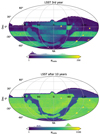 |
Fig. 1. LSST survey footprint showing the number of visits (Nvisits) in each sky location. The top panel shows the visits during the third year when the rolling cadence is active, and the bottom pabnel shows the survey as expected after completion (ten years of observations). |
2.3. Supernova simulations
We generated synthetic SN light curves using the snsim2 python library, as previously done in Carreres et al. (2023) and Carreres et al. (2025b). This code allows us to simulate realistic LSST SN light curves and parameters on top of the mocks described in Sect. 2.1. The SN host galaxies are randomly selected inside the LSST footprint from the Uchuu mocks. The SN light curves were generated starting from a spectral energy distribution (SED) model including astrophysical effects: PVs effect on the redshifts, beaming due to the effect of PVs (Davis et al. 2011), and Milky Way extinction3. Hence, the SN observed redshifts and magnitudes are affected by correlated PVs due to the large-scale structure of each galaxy mock. In this analysis, we neglect any type of correlation between the SN rates and the host-galaxy properties (e.g., mass, star formation rate, star formation history). The effect of these correlations on the fσ8 measurement will be studied in future works.
We generated the true light-curve fluxes for each SN by integrating the SED models over the LSST filters4. The true fluxes are converted into observed fluxes and relative uncertainties using the observing conditions given by the OpSim simulation, described in Sect. 2.2. The flux uncertainties are estimated as the quadratic sum of the sky noise, the Poisson noise from the source, the noise from the host-galaxy surface brightness and the error on the zero point (ZP) estimation. We set σZP = 0.005 mag as a calibration uncertainty; this uncertainty will be refined in further works, together with studies on the impact of calibration uniformity on the fσ8 measurement.
In the following subsections, we describe the details and assumptions used to simulate different types of SNe.
2.3.1. Normal SNe Ia
Our simulation is primarily composed of normal SNe Ia, or just SNe Ia, the supernovae that are standardizable candles and are used in cosmological analyses. To simulate the normal SNe Ia we utilize the SALT3 SED model (Kenworthy et al. 2021). The SNe Ia are randomly assigned to the host galaxies in the Uchuu mocks following the redshift distribution given by the volumetric rate presented in Frohmaier et al. (2019), which is rescaled for the value of H0 in the Uchuu simulation. In our simulations we model the stretch distribution, x1, following the redshift-dependent two-Gaussian mixture from Nicolas et al. (2021) and the color distribution, c, using the asymmetric model described in Scolnic & Kessler (2016). The SN Ia intrinsic scattering is drawn from a normal distribution with a fixed dispersion equal to σM = 0.12 mag. The analysis of the effect of different intrinsic scatter models, such as the color-dependent one described in Brout & Scolnic (2021), is presented in Carreres et al. (2025a). Finally, for each SN Ia we compute the apparent magnitude using the Tripp formula (Tripp 1998),
 (2)
(2)
where μi is the distance modulus of each SN Ia. α and β are the coefficients that relate the stretch and the color to the magnitude for the whole SN Ia population. M0 is the SN Ia intrinsic brightness, which is rescaled by the H0 value in the Uchuu simulation. The values of the Tripp input parameters in the simulation are: α = 0.14, β = 2.9, and M0 = −19.12 mag.
2.3.2. Peculiar SNe Ia
We also simulated two types of peculiar SNe Ia that are contaminants in SN Ia samples: SN1991bg-like SNe (Filippenko et al. 1992, hereafter SNe 91bg-like) and SN2002cx-like supernovae (Li et al. 2003; Foley et al. 2013, hereafter SNe Iax).
SNe 91bg-like are subluminous compared to normal SNe Ia, they are characterized by smaller x1 (fast-declining), and are redder at peak than normal SNe Ia. In our simulations, we used the corrected SED library of 35 91bg-like events from the Photometric LSST Astronomical Time Series Classification Challenge5 (PLAsTiCC; Kessler et al. 2019). As in Kessler et al. (2019), we assume that the SN 91bg-like volumetric rate is 12% of the SN Ia rate.
SNe Iax generally rise and decline faster than normal SNe Ia. Again, we use the models presented in PLAsTiCC, which are based on SN 2005hk (Phillips et al. 2007). As in Vincenzi et al. (2021), to reproduce the color diversity of SNe Iax we apply a range of host extinctions in the simulations following the host-extinction distribution described in Rodney et al. (2014). Following Kessler et al. (2019), we assume the volumetric rate of SNe Iax at z = 0 to be 24% of the normal SN Ia rate and the redshift evolution of the SN Iax rate is chosen to follow the cosmic star formation rate from Madau & Dickinson (2014).
2.3.3. Core-collapse SNe
Our simulation of core-collapse SNe (hereafter SNe CC) is based on the library of 67 SED templates presented in Vincenzi et al. (2019). This library is created by combining spectroscopy and multi-band photometry of SNe CC across 6 different subclasses (SNIIP/L, SNIIb, SNIIn, SNIb, SNIc, and SNIc-BL). For the relative rate of each SN CC subtype, we use the measurements described in Shivvers et al. (2017). To simulate the redshift distribution we assume that the SN CC rate follows the cosmic star formation history from Madau & Dickinson (2014) normalized by the local SN rate measured by Frohmaier et al. (2020). We normalize the brightness of the SN CC templates using the Gaussian fit shown in Table 5 of Vincenzi et al. (2021). The values of the luminosity function for each SN CC subtype are computed in Vincenzi et al. (2019) using the measurement performed by Li et al. (2011) and the revised rates from Shivvers et al. (2017). In our simulation, we use the set of templates from Vincenzi et al. (2019) that have not been corrected for host-galaxy dust extinction because the luminosity functions are also measured from SNe that were not corrected for host-galaxy dust extinction.
2.3.4. snsim output
snsim outputs the observed fluxes and simulated parameters of each SN. In simulating LSST, we apply a cut on the sampling of the light curves. We simulate the SNe with at least 10 observations within −50 < t0 < 150 days in any band. This selection is applied to ensure a minimum sampling of the light curves, speed up the simulations and reduce the data storage. We perform tests changing this initial cut and conclude that this selection does not affect the results of this analysis. Moreover, by computing the selection function of the simulation output with respect to the parent sample given by the assumed rate, we verify that the initial simulated sample is complete in redshift. The average number of SNe in our LSST simulations is ⟨N⟩ = 318 579. We highlight that all the results that we show in this work strongly depend on the assumptions made for the simulation, especially on the rates for the different SN types. To assess the real impact of contamination and selections on the growth rate, it will be necessary to calibrate the simulations on the first year of LSST data. This means creating simulations that reproduce the parameter distributions of the real data, as done in Vincenzi et al. (2021).
2.4. Light-curve selection
After simulating the SN light curves, as described in the previous section, we apply a series of selections to construct the expected sample that will be detected by LSST:
-
We remove all the saturated observations using the nominal LSST saturation limit6 (we did not account for changes in the saturation limit due to different observing conditions, e.g., different seeing conditions).
-
We apply the detection probability expected from the Difference Image Analysis (DIA) LSST-DESC pipeline. We use the detection efficiency as a function of the signal-to-noise ratio (S/N), as shown in Figure 9 of Sánchez et al. (2022). We keep in our sample all the light curves that have at least one detected observation in any band.
-
To determine which SNe will have a host galaxy with measured spectroscopic redshift, we apply host spectroscopic redshift efficiencies from the Dark Energy Survey Instrument (DESI) and the 4-metre Multi-Object Spectroscopic Telescope (4MOST). In Sect. 2.5 we describe how those efficiencies have been computed. Naturally, we select only the SNe that are observed by LSST and lie inside the DESI and 4MOST footprints.
-
We coadd the observations per night. Some light curves have two or more separated observations taken in the same night through the same filter, so we merge those observations into a single one and recompute the S/N. Finally, we keep in the sample the light curves that have S/N > 4 in at least three distinct bands.
2.5. Host spectroscopic redshift selection
We determine the efficiencies of the DESI Bright Galaxy survey Sample (BGS), 4MOST Cosmology Redshift Survey bright galaxies (CRS-BG) and 4MOST Hemisphere Survey of the Nearby Universe (4HS) surveys to obtain the spectroscopic redshifts of SN host galaxies. We define the SN-host redshift efficiency, Rhost as the ability of a spectroscopic survey to measure the redshift of an LSST SN host. For each SN type, the efficiency can be mathematically characterized by the number of LSST SN hosts whose redshifts are measured normalized by the total number of SNe. We assume that Rhost can be decomposed as:
 (3)
(3)
where Rspectro is the survey redshift efficiency, and RSN is the proportion of SNe located in the targeted hosts with respect to the total number of SNe.
To compute Rhost we use the DESC DC2 simulations (Abolfathi et al. 2021) and, in particular, the associated LSST-Roman OpenUniverse catalog (OpenUniverse et al. 2025), described in Sect. 2.1.
2.5.1. Computing Rspectro.
For each survey, we use the corresponding magnitude and color cuts that define the target galaxy sample. The target galaxies are similar for the three considered surveys, since at low redshifts all the surveys target Bright Galaxies (BGs). We apply the target selection cuts on the galaxies inside cosmoDC2 simulation. By normalizing the galaxy density as a function of redshift inside cosmoDC2, nDC2(z), by the expected n(z) of each survey, we estimate the corresponding survey redshift efficiency, Rspectro as a function of redshift. The DESI n(z) is obtained from the public information of the target selection in Hahn et al. (2023). Further information about target selection for the 4MOST surveys is obtained from Taylor et al. (2023) and Richard et al. (2019) and complemented with the expected n(z).7. The details on the target selection of each survey are described in Appendix A.
2.5.2. Computing RSN.
We use the galaxy properties in the simulation, such as stellar mass and star formation rate, to simulate the SNe and assign them to the most probable host. We apply the galaxy target selection cuts of each survey to the SNe simulated in the cosmoDC2 simulation and we normalize by the total number of SNe. This provides an estimation of the proportion of SNe located in the targeted host, RSN. The details on the SN simulation inside cosmoDC2 are described in Appendix A.
2.5.3. Rhost results.
Finally, we compute Rhost following Eq. (3) for each survey. We compute Rhost only as a function of redshift, assuming that it does not vary inside the survey footprints8.
The SN-host redshift efficiencies of DESI BGS, 4MOST CRS-BG and 4HS for all the SN types in our simulations are given in Fig. 2, which does not show the number of hosts observed but rather the proportion. A low proportion can represent a large number of host-galaxy redshifts, especially at high redshifts where the volume is larger. The efficiencies are different for each SN type since different types of SNe tend to occur in galaxies with distinct properties. We note that the DESI BGS and 4MOST HS have a high efficiency (almost one) for SNe Ia at z < 0.1. The high efficiency means that for z < 0.1 we will be able to get the spectroscopic redshift for almost all the SN Ia host galaxies, provided they are in the footprint of the surveys.
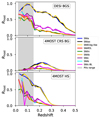 |
Fig. 2. SN-host redshift efficiencies, Rhost, as a function of redshift for each type of SN in the simulation. The top panel shows the efficiencies for DESI BGS survey, the central panel shows the ones for 4MOST CRS BG survey and the bottom panel shows the efficiencies for 4MOST 4HS surveys. The gray shaded area shows the redshift range of interest for LSST PV measurement. |
2.6. Photometric classification
After applying the selections described above, the next step of the analysis is the SN classification. LSST will discover an unprecedented number of supernovae, exceeding the resources available to acquire SNe spectra. The 4MOST Time-Domain Extragalactic Survey (TiDES, Swann et al. 2019) will provide spectroscopic follow-up only for ∼30 000 SNe at all redshifts (Frohmaier et al. 2025). Hence, a large part of the LSST SNe will not have a spectroscopic classification. LSST will rely on photometric classifiers: machine learning models trained on light curves to infer the SN types.
In this work, we use the SuperNNova (SNN; Möller & de Boissière 2019) framework to perform photometric classification of our simulated SN datasets and measure for each SN event its probability of being a SN Ia (PIa). We chose SNN since the code is publicly available9 and has been used for the Dark Energy Survey (DES) year 5 cosmological analysis (Vincenzi et al. 2024; DESI Collaboration 2024). To train SNN we run a new simulation of the LSST 10-year sample using the same inputs described in Sect. 2.3. We apply all the selections described in Sect. 2.4 to have a training sample that is representative of the SNe we want to classify. Since SNN needs a large training sample, simulations have typically been used to train the model (see Vincenzi et al. 2024). Because the SALT3 model we use to simulate the SNe Ia is defined in the phase range −20 < t0 < 50, we restrict the light curves for each SN type in our training sample. We define t0 as the time of the observation with maximum flux in any band within all the observations with S/N> 4. This cut is implemented because the classifier may otherwise learn that any observation outside the range −20 < t0 < 50 indicates the object is not a SN Ia, which is not realistic for real data. Additionally, we kept only light curves with at least ten observations in this phase range in the training set to ensure well-sampled light curves. The final training sample is composed of about 50 000 SNe Ia and about 18 000 contaminants. In the case of the binary classification task SNN maximizes the accuracy, so the classifier needs a balanced training sample (Möller & de Boissière 2019). SNN automatically downsamples the class with the highest number of objects in the training sample, so at the end, we train the classifier with about 36 000 objects (half SNe Ia and the other half for all the other types). To train the classifier we use the same hyperparameters as Möller & de Boissière (2019) and Vincenzi et al. (2021) and we add the spectroscopic redshift information. Additionally, we normalize the input fluxes using the “cosmo” flag, where each SN multi-band light curve is normalized independently and the normalization factor is the SN maximum flux in any filter. In Sect. 2.8.3 we show the classification metrics and results obtained using SNN on our eight LSST realizations.
2.7. Light-curve fit and quality cuts
The fit of each SN light curve is performed using the same framework as was used to generate the SNe Ia (SALT3). For each light curve, we fit the stretch, x1, color c, peak apparent magnitude, mB, and time of peak brightness, t0. We assume that the error on the observed redshifts is negligible. We perform the light-curve fit on all observations within −15 < t0 < 45. The covariance matrix CSALT, i of the SALT fit is defined as:
 (4)
(4)
which is used to fit the standardization parameters and recover the PVs, see Sect. 3.1.
After the light-curve fits, we apply quality cuts to ensure the robustness of the fit results10. Considering the resulting χ2 and the degrees of freedom of each light-curve fit, we select only the best-fit models describing the data with a probability larger than 95%. To ensure a robust estimate of mB, we select light curves that contain at least three observations within −10 < t0 < 10 days. We discard any SN with best-fit stretch |x1|> 3 or color |c|> 0.3. Finally, we exclude objects for which the uncertainty on t0 or x1 is larger than 1, or the uncertainty on c is larger than 0.05.
2.8. The final samples
In the following sections, we describe the final SN samples that we recover after applying the selections we have described in the previous sections. We create different scenarios for the LSST SN survey to perform the fσ8 measurement and deliver the forecasts under different conditions. In the next sections we present those scenarios, the assumptions made to construct each of them, and the characteristics of each sample. The samples are presented from the most optimistic to the most realistic one.
Our simulations do not take into account the time needed to generate the galaxy templates for the DIA pipeline. The template generation strategy affects the light-curve quality and the detection efficiency during the first months of the survey (Street et al. 2020). Different template generation strategies can slightly change the number of SNe Ia reported in this work.
2.8.1. Full sample
For the most idealized scenario, we create a pure sample of SNe Ia. On this sample we perform the selections described in Sect. 2.4, except for the host spectroscopic redshift efficiency (Sect. 2.5). We perform the SALT fit on all the light curves that have passed our first selection and we apply the cuts on the fit results, as described in Sect. 2.7. In this scenario we assume that LSST will have unlimited external spectroscopic resources to acquire SNe Ia and their host spectra all over the footprint. We create this ideal scenario to understand the completeness of the survey given the ability to detect the SNe Ia and to show the full potential of LSST. Hereafter, we call this scenario the Full sample.
After all the selections, the average sample over 8 LSST realizations contains ⟨N⟩ = 52 326 SNe Ia up to z = 0.16. We analyze SNe up to z = 0.16 because the Uchuu mocks have a maximum redshift of z ∼ 0.17 (Sect. 2.1), so we cut the SN samples before the mock limits to avoid possible artifacts in the PV field at the mock edges. We remind the reader that the maximum redshift for PV studies is z ∼ 0.2 because for higher redshifts the PV effect on the redshift is too small to be properly measured (Strauss & Willick 1995). Figure 3a shows the number density of SNe Ia in the Full sample across the sky. Figure 3b shows that the SN Ia number is uniform inside the WFD area, as expected, while we lose SNe Ia around the galactic plane due to the lower light-curve sampling and dust extinction.
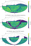 |
Fig. 3. Density maps of the different SN Ia samples across the LSST footprint. SN density in the initial simulated sample (a), density of the Full sample (b), and density of the Spec-z sample (c). All the maps represent the average over the eight LSST realizations. |
Figure 4 shows the SN Ia average redshift distribution (top panel), comoving density (middle panel), and redshift completeness for the Full sample. The density of the Full sample after detection and after the SALT fit increases at low redshift up until z ∼ 0.025. This means that at extremely low redshift we lose SNe Ia due to selection effects caused mainly by the saturation of the camera. There are about 100 SNe Ia with at least one saturated observation for z < 0.025. The effect of saturation is confirmed in the redshift completeness plot where we clearly see selections at low redshift. Naturally, if LSST discovers those SNe at early time, before they reach the maximum and saturate, they can be followed up by other surveys such as La Silla Schmidt Southern Survey (LS4, Miller et al. 2025). The redshift completeness plot shows that we lose SNe Ia for redshifts higher than ∼0.08. At higher redshifts we lose the dimmer SNe Ia. In Sect. 4 we discuss how the selection at higher redshift affects the growth-rate measurement.
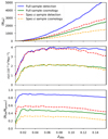 |
Fig. 4. Redshift distribution (top panel), comoving density (middle panel), and redshift completeness (bottom panel) for the Full and Spec-z samples. The Full sample detection and Spec-z sample detection show the results for the samples before running the SALT fit. The Full sample cosmology and Spec-z sample cosmology present the samples after the quality cuts on the SALT fit results. All the results are the average over the eight LSST realizations. The completeness distributions are computed with respect to the initial simulated sample (considering only the SNe Ia). |
2.8.2. Spec-z sample
For a more realistic scenario we create a pure sample of SNe Ia, but we apply all the selections of Sect. 2.4, including the host spectroscopic redshift. We perform the SALT fit on all the light curves that have passed our first round of selections and we apply the same cuts on the fit results as before. In this scenario we assume that LSST will make use of the observations of DESI and 4MOST to get the spectroscopic redshifts of the SN Ia host galaxies. We also assume that LSST will have unlimited external resources to acquire SN spectra within the DESI and 4MOST footprints. This scenario is created to deliver a realistic forecast for the growth rate from LSST SNe Ia without worrying about possible biases due to contamination. In this case we want to show the realistic statistical power of LSST and to understand the synergies with other facilities. Hereafter, we call this scenario the Spec-z sample. We highlight that in an analysis with real data, a fraction of the SNe Ia will be associated with the wrong galaxy, so those SNe Ia will be attributed a wrong redshift. In the Dark Energy Survey 5-Year (DES-SN5YR) photometric sample analysis the percentage of host mismatch was found to be about 1.7%, see (Qu et al. 2024). The mismatch causes a small systematic error in the final cosmology measurement because of the wrong redshifts assigned to the SNe. In this analysis we do not consider any SN Ia host mismatch and we leave the study of the impact of this mismatch on the fσ8 measurement to future works.
After all the selections, the average Spec-z sample over 8 LSST realizations contains ⟨N⟩ = 33 682 SNe Ia up to z = 0.16. Figure 3b shows the number density of SNe Ia across the sky. Figure 3b shows the SNe Ia that lie inside the intersection between the LSST footprint and DESI + 4MOST footprints, thus the region around the galactic plane is completely empty.
Figure 4 shows the average SN Ia redshift distribution (top panel), comoving density (middle panel), and redshift completeness for the Spec-z sample. Like the Full sample the density increases at low redshift up until z ∼ 0.025 due the selection caused by saturation at extreme low redshift. The comoving density of the Spec-z sample is similar to that of the Full sample one up to z ∼ 0.12. This means that we will have the spectroscopic redshift for almost all the SN Ia host galaxies up to that redshift. In fact, the host-spectrum efficiencies are almost one for DESI BGS and 4MOST HS at low redshift, see Fig. 2. The host-spectroscopic efficiencies start to decrease for z > 0.12, so the density of the Spec-z sample is lower than that of the Full sample. The redshift completeness shows that the Spec-z sample also becomes incomplete above z ∼ 0.08.
In Sect. 4.3 we show and discuss our results of the growth-rate measurement for the Spec-z sample.
2.8.3. Photo-typed sample
For the most realistic scenario, we simulated all of the SN types described in Sect. 2.3. We apply all the selections described in Sect. 2.4, including the host spectroscopic redshift efficiency, and we classify the SNe using SNN (Sect. 2.6). Hereafter, we call this sample the Photo-typed sample.
Within the SNN binary classification framework that separates SNe Ia from the other SN types, we define correctly classified SNe Ia as true positives (TP), while correctly-classified contaminant supernovae are true negatives (TN). Misclassified instances, where SNe Ia are identified as CC or vice versa, are treated as false negatives (FN) and false positives (FP) respectively. The classification is based on the highest-probability prediction, so an object is classified as SN Ia if the probability given by SNN is PIa > 0.5. To evaluate the effectiveness of our classification method, we focus on two primary performance metrics: contamination fraction and classification efficiency. The contamination represents the fraction of non-SNe Ia among all events classified as SN Ia, and is defined as:
 (5)
(5)
so a good classification means low contamination. The classification efficiency measures the percentage of actual SNe Ia that were successfully identified and is defined as:
 (6)
(6)
so a good classification means high efficiency.
From SNN classification we initially identify a sample of ⟨N⟩ = 68 084 SN candidates as likely SNe Ia. We find a classification efficiency of 92.3 ± 0.1%, with contamination fraction at 1.15 ± 0.04% (these values are the mean over the eight LSST realizations and the errors are the standard deviations). By imposing additional quality selection through SALT fit cuts (Sect. 2.7), this sample is refined to ⟨N⟩ = 33 269 SNe. The resulting contamination fraction for this more stringent sample is 0.021 ± 0.007%. The small contamination demonstrates the strength of SNN in performing photometric classification for a low-z SN sample. The contamination fraction is lower than has been seen before. The low contamination may be a result of the fact that we are analyzing only low-redshift SNe, but a proper investigation of this is beyond the scope of this work and we leave it for future studies.
For this sample we do not show the number density across the sky and the SNe redshift distribution because they are not significantly different from the Spec-z sample and all comments given in the previous section are still valid.
In Appendix B we describe the performance comparison between SNN and the Parsnip classifier (Boone 2021). There we show that the classifier performances strongly agree, so we can conclude that the SNN classifier is reliable in the context of the simulations used in this work.
3. Method
In this section we describe the method we employed to measure fσ8 using the PVs derived from the SN samples described in Sect. 2.8. In this analysis we use the maximum likelihood method which assumes that the PV field is drawn from a multivariate Gaussian distribution. This method has been used in past works by Johnson et al. (2014), Adams & Blake (2020), Lai et al. (2023), Carreres et al. (2023) who applied the maximum likelihood method to samples of PVs derived from SNe Ia, TF, and FP galaxies.
The likelihood is a multivariate Gaussian that is expressed as
![Mathematical equation: $$ \begin{aligned} \begin{aligned} L (f\sigma _8,\Theta ,\Theta _{\mathrm{HD} } ) = (2\pi )^{-\frac{n}{2}} |C(f\sigma _8,\Theta ,\Theta _{\mathrm{HD} } )|^{-\frac{1}{2}} \\ \times \exp \left[ -\frac{1}{2} \mathbf v ^T(\Theta _{\mathrm{HD} }) C(f\sigma _8,\Theta ,\Theta _{\mathrm{HD} } )^{-1} \boldsymbol{v}(\Theta _{\mathrm{HD} }) \right] \,, \end{aligned} \end{aligned} $$](/articles/aa/full_html/2025/09/aa56181-25/aa56181-25-eq7.gif) (7)
(7)
where v is the velocity data vector, Θ is the vector of the nuisance parameters, and ΘHD is the vector of the Hubble diagram (HD) standardization parameters. C(fσ8, Θ, ΘHD) is the covariance matrix that describes the correlations between the PVs and includes the measurement errors.
In this section we present in detail all the components of the likelihood and the parameters of the model: in Sect. 3.1 we describe how we measure the PVs from the HD residual and in Sect. 3.2 we explain the construction of the covariance matrix.
3.1. Estimating the peculiar velocities
The SN Ia host-PVs can be estimated using the residual of the HD after standardization. The SN Ia standardization process is the minimization of the residuals of the distance modulus μi to the HD, using the Tripp relation, given in Eq. (2). We define the parameter vector that contains the HD standardization parameters as ΘHD = (α, β, M0).
To estimate the host-galaxy PVs we make use of the HD residuals, which are the difference between the observed distance modulus and the distance modulus given by the cosmological model and evaluated at the observed redshift of each SN. The residuals are given by
 (8)
(8)
and their uncertainties
 (9)
(9)
where CSALT, i is the SALT covariance, defined in Eq. (4), σM2 is the SN intrinsic scatter and AT = (α, −β, 1).
Carreres et al. (2023), following Hui & Greene (2006), demonstrates that the first-order expansion of HD residuals with respect to the PVs gives the following estimator:
 (10)
(10)
where H(z) is the Hubble parameter and r(z) is the comoving distance, which is defined as:
 (11)
(11)
Naturally, the estimator gives the host-galaxy PV along the line of sight only. The uncertainty on the velocity estimation is:
 (12)
(12)
3.2. Covariance matrix
The covariance matrix in Eq. (7) is defined as:
![Mathematical equation: $$ \begin{aligned} \begin{aligned} C_{ij}(f\sigma _8,\Theta ,\Theta _{\mathrm{HD} })&= C^{vv}_{ij} (f\sigma _8, \sigma _u) \\&+[\sigma ^2_v + \sigma ^2_{v,i}(\Theta _{\mathrm{HD} },\sigma _M)] \delta ^K_{i,j}\,, \end{aligned} \end{aligned} $$](/articles/aa/full_html/2025/09/aa56181-25/aa56181-25-eq13.gif) (13)
(13)
where Cvv is the analytical part that depends on fσ8 and σu, σv, i2 is the error on the velocity estimator defined in Eq. (12), and σv2 is a nuisance parameter to take into account the extra scatter due to the imperfect modeling of nonlinear scales. The parameter σu is used to model the RSD and is defined later in this Section. Hereafter, we define the vector of the nuisance parameters as Θ = (σu, σv, σM).
The covariance Cvv represents the correlation of the velocity field between the positions ri and rj. In the general case we can define  , where v is the 3D velocity vector. The radial component vi of the 3D velocity field at a position ri in Fourier space can be written as:
 (14)
(14)
Therefore, the covariance can be defined as:
 (15)
(15)
We can rewrite Eq. (15) using the velocity divergence scalar field, θ(r), defined as:
 (16)
(16)
where a is the scale factor and H(a) is the Hubble parameter. Assuming that the velocity field is irrotational, in Fourier space we obtain:
 (17)
(17)
Using the divergence field we can define the velocity-divergence auto power spectrum as ⟨θ(k)θ*(k′)⟩ = (2π)3δD(k − k′)Pθθ(k). At this point we can use the velocity-divergence auto power spectrum to simplify Eq. (15); the resulting Cvv is given by:
 (18)
(18)
for the full derivation of the velocity covariance see Johnson et al. (2014), Carreres et al. (2023) and references therein. In Eq. (18), Wij(k; ri, rj) is the so-called window function, which is defined as (see Ma et al. 2011):
![Mathematical equation: $$ \begin{aligned} \begin{aligned} W_{ij}(k;\mathbf r _i,\mathbf r _j)&= \frac{1}{3} \left[ j_0 (k r_{ij}) -2 j_2 (k r_{ij}) \right] \cos (\phi _{ij}) \\&+ \frac{1}{r_{ij}^2} j_2 (k r_{ij}) r_i r_j \sin ^2(\phi _{ij}), \end{aligned} \end{aligned} $$](/articles/aa/full_html/2025/09/aa56181-25/aa56181-25-eq20.gif) (19)
(19)
where ϕij is the angle between ri and rj, rij = |ri–rj|, j0 and j2 are the zeroth and second order spherical Bessel functions respectively.
In this work we compute Pθθ using the cosmological parameters of the Uchuu simulation, and we normalize the power spectrum for σ8, fid2. For our mocks σ8, fid = 0.8159. To compute Cvv we use the empirical non linear model of Pθθ from Bel et al. (2019). This model is built by parametrizing the velocity-divergence power spectrum as Pθθ = Pθθ, linexp[−k(a1 + a2k + a3k2)], where a1, a2, a3 are coefficients fitted in simulations and depend linearly on σ8. Pθθ, lin is the linear velocity-divergence power spectrum, which is equal to the linear density-density power spectrum and is computed using the Boltzmann solver CAMB11 (Lewis et al. 2000). Carreres et al. (2023) performed an accurate investigation on the impact of various Pθθ models on the fσ8 measurement. From the results of that work, we conclude that the approximation from Bel et al. (2019) is a good enough model for the velocity-divergence power spectrum.
To calculate Cvv we compute the comoving distances r, which are estimated using the observed redshifts, hence the distances are affected by PVs. Therefore, we have to take into account the RSD in our model for Cvv. We model the RSD using the empirical damping on the Pθθ small scales from Koda et al. (2014). The damping is given by:
 (20)
(20)
and is based on N-body simulations.
In this work Cvv is computed at z = 0 since the Uchuu mocks come from a snapshot at that redshift. Hence
 (21)
(21)
where fσ8, fid is the value of the growth rate from the Uchuu simulation and ffid ≃ Ωm0.55. We highlight that with the maximum likelihood method we fit for the value of  . kmin and kmax are the minimum and maximum scales between which the power spectrum is computed. In the covariance computation we set kmax = 1 h Mpc−1 to ensure convergence (see Appendix B in Carreres et al. 2023) and kmin is imposed by the size of the N-body simulation box: kmin = 2π/Lbox = 4.6 × 10⁻³h Mpc−1. To compute the covariance given by Eq. (21) we use the FLIP12 python package. The FLIP framework and the full derivation of the covariance matrix formula are presented in detail in Ravoux et al. (2025). To find the maximum likelihood we use the gradient descent algorithm iminuit13 (Dembinski et al. 2023). In Appendix C we show systematic tests which demonstrate the reliability of the maximum likelihood method.
4. Results
In this section, we describe the main results of this work. Before measuring fσ8 we check for any potential biases that could arise from our sample selection criteria (Sect. 4.1). After that, we use the maximum likelihood approach (Sect. 3) to measure fσ8 in different redshift bins for all the SN samples described in Sect. 2.8: see Sect. 4.2 for the Full sample, Sect. 4.3 for the Spec-z sample, and Sect. 4.4 for the Photo-typed sample.
4.1. Selection effect on the Hubble residuals and estimated velocities
Carreres et al. (2023) shows that the Malmquist bias heavily affects the growth-rate measurement through PVs since the likelihood in Eq. (7) does not take into account selection effects. As shown in Fig. 4, at z ∼ 0.08 all our SN samples start to be affected by Malmquist bias. Therefore, to ensure that the final measurement will not be biased, we check the HD residuals and the estimated velocities as a function of redshift. In future works we will study how to correct for this type of selection bias using already existing method like BEAMS with Bias Corrections (BBC, Kessler & Scolnic 2017), UNITY (Rubin et al. 2015, 2025), or directly modifying the likelihood as shown in Kim (2020).
Figure 5 shows the Full sample HD residuals as a function of the observed redshift (top panel) and as a function of the cosmological one (bottom panel). The HD residuals are computed using the input simulation values and the reference cosmology. We observe a trend in the HD residuals as a function of zobs that follow the mean of the true galaxy PVs. When the HD residuals are plotted against zcos, the trend disappears, indicating that PVs are responsible for the deviations in the residuals relative to zobs. The standard deviation of 8 mocks (red points) is higher than the mean error over the stacking (blue points). This happens when the covariance due to PVs is not accounted for, as already shown in Carreres et al. (2025b). The discrepancy in the distance modulus residuals is evident at low redshift (z < 0.1) and disappears at higher redshift, as the PV contribution becomes subdominant. The bottom panel of Fig. 5 shows a large reverse Malmquist bias for z < 0.02, due to saturation effects, since the brighter objects are removed.
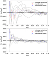 |
Fig. 5. Hubble diagram residuals as a function of the observed redshift (top panel) and cosmological redshift (bottom panel) for the Full sample. The solid gray lines show the residual for each of the eight LSST realizations, the red points show the mean of the eight mocks, and the blue points show the mean computed by stacking all the mocks. |
To ensure that the growth-rate measurement will not be biased we also check the PV residual. Figure 6 shows the difference between the PVs estimated from the HD residuals of Fig. 5 and the true velocities as a function of the observed redshift. The PV residuals show a small bias for z < 0.02 and z > 0.08, the same range where the HD residuals are biased, as expected. The maximum PV bias is around 70 km s−1 , which is almost one order of magnitude smaller than the PV measurement error in this redshift range. Therefore, we do not expect any significant bias on the growth-rate measurement.
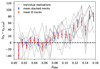 |
Fig. 6. Difference between estimated PVs (vp) and true PVs (vp, true) as a function of the observed redshift for the Full sample. The solid gray lines shows the residual for each of the eight LSST realizations, the red points are the means over the eight mocks, and the blue points show the means computed by stacking all the mocks. |
Considering the results on the PV bias, shown in Fig. 6, we choose to perform the growth-rate measurement within the redshift range 0.02 < z < 0.14 for all the samples described in Sect. 2.8. The low-redshift cut is applied for two main reasons: to avoid the region where we have selection effects due to saturation and to avoid our PVs being correlated with the local structure nearby the observer, so we analyse only SNe which live inside the Hubble flow. The high redshift cut is applied to avoid the redshift range where the bias in PVs reaches about 100 km s−1. Figure 5 and Fig. 6 show the Full sample residual plots only. We do not show the HD and PV residuals for the Spec-z and Photo-typed sample since the results are almost identical to those of the Full sample.
4.2. Full sample
In this section we present the results of the growth-rate measurements from the PVs inferred from the Full sample, described in Sect. 2.8.1. We measure the growth-rate parameter in different redshift bins. We use volume bins to show the full statistical power of the LSST dataset going towards higher redshift. This means that for each redshift bin we use the same minimum redshift (zmin = 0.02) and increase the maximum redshift. We also measure the growth rate in tomographic bins to show the precision with which LSST PVs can explore the redshift dependence of fσ8. When using the tomographic bins the correlations on the largest scales are not taken into account so the constraining power of the total sample decreases. Estimating fσ8 as a function of redshift (in tomographic bins) allows us to measure the so-called “growth index” γ (see for example Nguyen et al. 2023).
Figure 7 and Table 1 shows the fit results for each mock (top panel) and the relative error (bottom panel) for each sample.
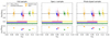 |
Fig. 7. Results of fσ8 measurements for all the scenarios in different redshift bins. Left: Full sample. Center: Spec-z sample. Right: Photo-typed sample. For each scenario, the top panel shows the results of the fit for each of the eight LSST realizations together with the mean value, and the bottom panel shows the mean values of σfσ8/fσ8, fid, which are the relative errors on the growth-rate measurements. The averages are plotted at the mean redshift positions, while the results for the individual realizations are slightly shifted along the abscissa for clarity. The colored bars show the redshift range used for each fσ8 measurement; the bars have the same colors as the measurements. |
Summary of the fσ8 results for all LSST scenarios.
We focus on the left panel of Fig. 7, which shows the results for the Full sample. We notice that the averages are always compatible with the fiducial value, except for the redshift range 0.06 < z < 0.1. The discrepancy between the true fσ8 and the recovered one in that redshift bin is less than 2-σ for each realization. The small discrepancy is probably caused by sample variance. To confirm this, more than eight realizations are needed, so we leave this investigation for future works. The mean reduced χ2 is about one in each bin, except in the redshift range 0.06 < z < 0.1 where the mean reduced χ2 is ∼1.3, which confirms the robustness of the fits. From the study of the optimistic Full sample we can appreciate the full statistical power of LSST data to constrain the growth rate using SN Ia PVs reaching an 8% precision in the redshift range 0.02 < z < 0.14. Moreover, in the most optimistic case we will be able to constrain the parameter to 12% precision using tomographic bins. The results described in this section demonstrate that the small bias in the PV residual, see Sect. 4.1, does not impact the growth-rate measurement. The small Malmquist bias does not impact the growth-rate measurements obtained with the Spec-z sample and the Photo-typed sample, as shown in the next sections. The Malmquist bias affects the fit results for the HD parameters, as described in Appendix D.
4.3. Spec-z sample
We present the growth-rate measurement using the PVs measured from the Spec-z sample, described in Sect. 2.8.2. Figure 7 (central panel) and Table 1 show the fit results for the Spec-z sample. The recovered fσ8 are always compatible with the simulation input, except for the redshift bin 0.06 < z < 0.1 as in the previous case. For the Spec-z sample the mean reduced χ2 is about one in each bin, except in the redshift range 0.06 < z < 0.1 where the mean reduced χ2 is ∼1.2, which confirms the goodness of the fits. From the study of the Spec-z sample we can see that LSST, using the spectroscopic redshift from DESI and 4MOST, will be able to constrain the growth rate with 9% precision in the redshift range 0.02 < z < 0.14. Moreover, in this more realistic scenario the constraints on fσ8 reach 14% precision in the tomographic bins.
4.4. Photo-typed sample
In this section we describe the growth-rate measurement using the PVs measured from the Photo-typed sample described in Sect. 2.8.3. This is our baseline analysis and the most realistic LSST scenario.
The results for the growth-rate measurement using the Photo-typed sample are shown in Figure 7 (right panel) Table 1. Figure 7 shows that the averages are always compatible with the simulation input, except for the redshift bin 0.06 < z < 0.1 as in the previous cases. From the Figure we can conclude that in this scenario there is also no significant bias in the measurement and we are able to recover correctly the growth rate. Therefore, a low percentage of contamination in the HD does not bias fσ8 from PVs.
We note that in this scenario the error on fσ8 is systematically higher (1 − 2%) compared to the one for the Spec-z sample. This is caused by the slightly lower number of SNe Ia in the Photo-typed sample due to SNN inefficiencies, and by the extra scatter in the HD due to the contamination. To test this we perform two extra fits: one by removing the contaminants and the other by manually adding SNe Ia to reach the same numbers as in the Spec-z sample. In both cases, the average error of fσ8 is higher than that in the Spec-z sample, but not as large as in the Photo-typed sample. This test demonstrates that a low level of contamination does not bias the measurement but slightly increases the final error. In the next Section we show the effect of increasing contamination in the measurement of the growth-rate. Additionally, the mean reduced χ2 for the Photo-typed sample is ∼1.05 in each bin and ∼1.2 in the redshift range 0.06 < z < 0.1. These values demonstrate the goodness of the fits and are comparable to the ones of the Spec-z sample. From the study of the Photo-typed sample we can see that LSST will be able to constrain the growth rate with 10% precision in the redshift range 0.02 < z < 0.14. Moreover, we can constrain the fσ8 up to 14% precision in the tomographic bins.
In Appendix E, using the Photo-typed sample, we show forecasts for the expected error on the fσ8 across the LSST survey years of observation. We demonstrate that after 5 years of observation, we will be able to reach a precision of 12% in the redshift range 0.02 < z < 0.14.
5. Test of the contamination effect
In this section, we vary the sample contamination to determine the threshold at which the incorrect likelihood gives significantly biased results. To produce this variation we do not use SNN. In each new sample we use the SNe Ia inside the Spec-z sample and we vary the SN contamination14 by applying different quality cuts on the SALT fit results of the other SN types (as similarly done in Vincenzi et al. 2021).
Figure 8 illustrates the HD residuals and the residuals of the estimated velocities, normalized by the errors, for different samples with increasing contamination for one LSST realization. These residuals are computed using the input value of the simulation in the redshift range 0.02 < z < 0.14. Figure 8 shows that as the contamination increases, the distributions become more skewed. This can create a bias in the maximum likelihood, since the incorrect likelihood describes a Gaussian velocity distribution. To study when the method breaks, we perform the fσ8 fit on the samples with different contamination.
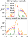 |
Fig. 8. HD residuals (top panel) and residuals of the estimated velocities (bottom panel), normalized by the errors, using the input HD parameters of the simulation. The plot shows the residuals for a random realization in the simulation in the redshift range 0.02 < z < 0.14. The different colors represent different SN samples with different levels of contamination, as shown in the legend. |
Figure 9 presents the fσ8 results, averaged over the 8 LSST realizations, as a function of contamination, for the redshift bin 0.02 < z < 0.14. As the level of contamination increases, the bias on the growth-rate measurement becomes larger, especially when including higher redshift SNe. The measurement error on fσ8 also increases as a function of the contamination in the sample, because of the higher scatter in the HD diagram, as explained in the previous section. Figure 9 shows that a contamination level above ∼2% breaks the likelihood model. As the contamination increases, the HD parameters become more biased. We highlight that for high contamination fraction (i.e. > 2%) the fit fails in some realizations and gives fσ8 ∼ 0. This is because the scatter in the HD diagram increases to the point where the information of the PV correlation is lost. We find the same results for the other redshift bins listed in Table 1. Additionally, we observe that the measurement error for the red point with the lowest contamination is smaller than the error with the Photo-typed sample (i.e. SNN), but still higher compared to the error of the pure SNe Ia. As explained in Sect. 4.4, the number of SNe Ia in the Photo-typed sample decreases, due to the efficiency of the SNN. The results shown in Fig. 9 emphasize the need to control contamination to ensure the accuracy of the cosmological parameter estimation.
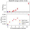 |
Fig. 9. fσ8 fit results (top panel) and relative error (bottom panel) as a function of the sample contamination fraction for the redshift bin 0.02 < z < 0.14. The blue points show the results for the Spec-z sample, the orange points show the Photo-typed sample, and the red points show the different samples created using the cuts on the SALT fits as classification (SALT cuts). Every point is the average over the eight LSST realizations. |
6. Discussion
Figure 10 illustrates the predicted evolution of the growth-rate parameter fσ8 as a function of redshift, comparing predictions from General Relativity (GR-ΛCDM) and alternative gravity theories. The Figure also shows forecasts for current and upcoming stage IV surveys like Euclid (Amendola et al. 2018), DESI (DESI Collaboration 2016; Saulder et al. 2023), and ZTF (Carreres et al. 2023).The blue crosses represent the LSST PV forecasts estimated in this analysis from the Photo-typed sample for the tomographic redshift bins. When compared with the results from ZTF PVs and DESI PVs, the forecast from LSST shows similar results for z < 0.06. LSST will obtain a precision similar to that of ZTF since both surveys will have a complete sample up to z < 0.06 with a similar number of SNe inside a similar volume. Fig. 10 also shows, however, that the LSST will obtain tighter constraints compared to DESI and ZTF for z > 0.06, and will therefore be able to more precisely measure the evolution of the growth-rate parameter with respect to the other surveys.
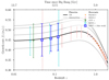 |
Fig. 10. Growth-rate parameter as a function of redshift. The solid black line shows the GR-ΛCDM prediction, and the gray lines present the predictions for alternative gravity theories. The points show different forecasts for future and current stage IV surveys. The orange points show the forecast for Euclid (Amendola et al. 2018), and the red circles show those for DESI (DESI Collaboration 2016). The forecasts from DESI and Euclid are derived from the analysis of the density field. The other forecasts come from the PV field: the green triangle from ZTF SNe Ia (Carreres et al. 2023), the cyan circles from the DESI PV survey (Saulder et al. 2023), and the blue crosses from LSST SNe Ia, which are the results from the Photo-typed sample in the tomographic bins. |
Compared to the forecasts by Howlett et al. (2017a), which report uncertainties smaller than 10% for z > 0.1, our forecasts show larger uncertainties. This difference arises because Howlett et al. (2017a) used a highly idealized LSST simulation that did not include the full selection process described in Sect. 2.4. As a result, their analysis included more SNe Ia than ours. Additionally, Howlett et al. (2017a) forecasts were based on the Fisher matrix method, which does not account for the survey footprint geometry (see Sect. 5 of Ravoux et al. 2025, for a comparison between Fisher matrix and maximum likelihood). In contrast, our approach is more realistic: we simulate the full LSST low-z sample, including selections and photometric classification, and extract constraints on fσ8, HD parameters, and nuisance parameters simultaneously using the maximum likelihood method, which better reflects how real data should be analyzed. Therefore, our results provide a more robust and realistic estimate of the expected uncertainties.
7. Conclusions
We demonstrated that the LSST SN sample can be a powerful dataset for measuring the growth rate of cosmic structures fσ8 through PVs. We simulated LSST light curves over ten years for various types of SNe (Sect. 2) using a realistic observing strategy that incorporated noise and the effect of the PV field from the Uchuu simulation. We created eight different realizations of the LSST ten-year survey using the detection efficiency of the DIA pipeline (Sect. 2.4) and the host spectroscopic redshift efficiency from DESI and 4MOST (Sect. 2.5).
We explored three scenarios: an idealized fully spectroscopic redshift sample, a spectroscopic sample combining LSST with DESI and 4MOST to obtain the SN host spectroscopic redshift, and a photometric sample incorporating a classification based on machine-learning (Sect. 2.6). These scenarios were built to assess the potential of LSST under various conditions and to distinguish possible systematics. For every scenario, we used the maximum likelihood method (Sect. 3) to obtain the growth-rate measurement using the PVs measured from the SN HD residuals.
In the most optimistic scenario, the Full sample, which contains ⟨52 326⟩ SNe Ia up to z = 0.16, we achieved the highest statistical precision for fσ8. The results demonstrated a uniform distribution on the sky within the WFD area (see Fig. 3b) and a nearly flat comoving density at low redshift, as shown in Fig. 4. The Full sample, as well as the others, showed a small Malmquist bias. This does not impact the final constraints on the growth rate (Sect. 4.1). For this sample, the measurement of fσ8 closely matches the input value of the simulation with a very low statistical error: 8% precision in the redshift range 0.02 < z < 0.14, and 12% precision for the tomographic bins (Sect. 4.2).
The Spec-z sample incorporates spectroscopic redshift efficiencies from DESI and 4MOST. It reduced the sample size to ⟨33 682⟩ SNe Ia because the overlapping sky coverage was limited (Fig. 3c). This sample maintained a high degree of uniformity within the overlapping survey footprints, and the comoving density was largely unaffected up to z = 0.12, as shown in Fig. 4. This scenario represents a realistic expectation of the LSST synergy with other spectroscopic surveys and yielded competitive constraints on fσ8 with a modest increase in the statistical uncertainties compared to the Full sample (see Sect. 4.3).
In the Photo-typed sample, we accounted for photometric classification using the SNN framework. Despite challenges such as sample contamination and efficiency limitations, the contamination fraction was successfully controlled at the level of 0.02% (Sect. 2.8.3). This indicates that SNN reliably handles simulated LSST data. The resulting fσ8 measurements, while slightly degraded compared to the spectroscopic samples, still provided valuable constraints on the growth rate and showed the capability of the LSST for an independent cosmological analysis without relying heavily on a spectroscopic follow-up of each SN Ia. After ten years of LSST, we will be able to constrain the growth-rate parameter at the 10% level using SN PVs alone. Moreover, we will be able to measure fσ8 with a 14% precision in the tomographic bins.
We also investigated the contamination effect that arises from the likelihood of Eq. (7) (see Sect. 5). We demonstrated that the method produces unbiased results, but with higher uncertainties, when the contamination is below ∼2%.
We highlighted the potential of the LSST PV sample to complement RSD measurements in general. It offers a robust and independent way for testing GR and different dark energy models. The combination of high- and low-redshift fσ8 measurements from the current survey generation opens the door to more precise measurement of the growth index γ (Nguyen et al. 2023). Future studies should focus on constructing a model-motivated likelihood to include selection effects, the HD residual correlation with the host galaxies and SN colors, and to incorporate the probability coming from the photometric classifier. These efforts will enhance the LSST contribution to precision cosmology. To further improve the constraints on the growth rate at low redshift, LSST PVs can be combined with other PV data from ZTF or DESI, and the LSST PV field can be cross-correlated with the density field from spectroscopic surveys (e.g., 4MOST and DESI).
CCM89 model Cardelli et al. 1989 dust law with RV = 3.1 and EBV from Schlegel et al. 1998.
For this operation we use the SNCOSMO package (https://sncosmo.readthedocs.io/).
u, g, r, i, z, y = 14.7, 15.7, 15.8, 15.8, 15.3, 13.9 mag values of LSST nominal saturation limit at 0.7″seeing from https://www.lsst.org/sites/default/files/docs/sciencebook/SB_3.pdf
Private communication from E. N. Taylor and J. Kneib, the principal investigators of each survey.
The code used to compute the SN-host efficiencies for this work is publicly available at https://github.com/corentinravoux/desidescsn
The quality cuts applied in this work are the ones which are commonly used for cosmological analyses.
The contamination is defined as the number of contaminants divided by the total number of SNe in the sample. This is the most natural definition for simulated objects as we know their true type.
When we refer to error we mean the realistic error expected from measuring PVs using SNe Ia and computed using Eq.(12).
Acknowledgments
This paper has undergone internal review in the LSST Dark Energy Science Collaboration. We thank the internal reviewers: Rebecca Chen and Erin Hayes. We would like to thank the anonymous referee for their valuable comments, which have helped improve the clarity and quality of the manuscript. Author contributions: D. Rosselli led the project, developed the simulation framework, performed the analysis, and wrote the manuscript. B. Carreres contributed to the development and validation of the galaxy mocks. C. Ravoux contributed to the determination of the host spectroscopic redshift efficiencies. C. Ravoux, B. Carreres, and A.G. Kim contributed to the velocity covariance modeling. J. E. Bautista provided support with plotting and reviewed the manuscript. D. Fouchez, F. Feinstein, B. Sánchez, and A. Valade contributed through manuscript review and critical feedback. B. Sánchez contributed to the light curve selection method and photometric classification task. B. Racine contributed to the analysis of the simulations. All authors contributed to the critical discussion of the results and reviewed the manuscript. This work was conducted within the LSST Dark Energy Science Collaboration, which provided the infrastructure, tools, and coordination essential to this study. Grants: The project leading to this publication has received funding from Excellence Initiative of Aix-Marseille University – A*MIDEX, a French “Investissements d’Avenir” program (AMX-20-CE-02 – DARKUNI). This work has been carried out thanks to the support of the DEEPDIP ANR project (ANR-19-CE31-0023). This work received support from the French government under the France 2030 investment plan, as part of the Initiative d’Excellence d’Aix-Marseille Université – A*MIDEX (AMX-19-IET-008 – IPhU). This work was performed using the Dark Energy Center (DEC) hosted at Aix Marseille Univ, CNRS/IN2P3, CPPM, Marseille, France. The DESC acknowledges ongoing support from the Institut National de Physique Nucléaire et de Physique des Particules in France; the Science & Technology Facilities Council in the United Kingdom; and the Department of Energy and the LSST Discovery Alliance in the United States. DESC uses resources of the IN2P3 Computing Center (CC-IN2P3–Lyon/Villeurbanne – France) funded by the Centre National de la Recherche Scientifique; the National Energy Research Scientific Computing Center, a DOE Office of Science User Facility supported by the Office of Science of the U.S. Department of Energy under Contract No. DE-AC02-05CH11231; STFC DiRAC HPC Facilities, funded by UK BEIS National E-infrastructure capital grants; and the UK particle physics grid, supported by the GridPP Collaboration. This work was performed in part under DOE Contract DE-C02-76SF00515. Codes: We acknowledge the use of numpy (Harris et al. 2020), scipy (Virtanen et al. 2020), and healpix (Gorski et al. 2005). Data availability: The data that support the findings of this study are available from the corresponding author upon reasonable request. Access to the data may be granted to researchers who are not LSST collaboration members, subject to applicable data sharing policies and guidelines.
References
- Abolfathi, B., Alonso, D., Armstrong, R., et al. 2021, ApJS, 253, 31 [CrossRef] [Google Scholar]
- Adams, C., & Blake, C. 2020, MNRAS, 494, 3275 [NASA ADS] [CrossRef] [Google Scholar]
- Alam, S., Aubert, M., Avila, S., et al. 2021, Phys. Rev. D, 103, 083533 [NASA ADS] [CrossRef] [Google Scholar]
- Amendola, L., Kunz, M., Saltas, I. D., & Sawicki, I. 2018, Phys. Rev. Lett., 120, 131101 [NASA ADS] [CrossRef] [Google Scholar]
- Aung, H., Nagai, D., Klypin, A., et al. 2023, MNRAS, 519, 1648 [Google Scholar]
- Behroozi, P., Wechsler, R. H., Hearin, A. P., & Conroy, C. 2019, MNRAS, 488, 3143 [NASA ADS] [CrossRef] [Google Scholar]
- Bel, J., Pezzotta, A., Carbone, C., Sefusatti, E., & Guzzo, L. 2019, A&A, 622, A109 [NASA ADS] [CrossRef] [EDP Sciences] [Google Scholar]
- Boone, K. 2021, AJ, 162, 275 [NASA ADS] [CrossRef] [Google Scholar]
- Brout, D., & Scolnic, D. 2021, ApJ, 909, 26 [NASA ADS] [CrossRef] [Google Scholar]
- Cardelli, J. A., Clayton, G. C., & Mathis, J. S. 1989, ApJ, 345, 245 [Google Scholar]
- Carreres, B., Bautista, J. E., Feinstein, F., et al. 2023, A&A, 674, A197 [NASA ADS] [CrossRef] [EDP Sciences] [Google Scholar]
- Carreres, B., Chen, R. C., Peterson, E. R., et al. 2025a, ArXiv e-prints [arXiv:2505.13290] [Google Scholar]
- Carreres, B., Rosselli, D., Bautista, J. E., et al. 2025b, A&A, 694, A8 [NASA ADS] [CrossRef] [EDP Sciences] [Google Scholar]
- Carrick, J., Turnbull, S. J., Lavaux, G., & Hudson, M. J. 2015, MNRAS, 450, 317 [Google Scholar]
- Davis, T. M., Hui, L., Frieman, J. A., et al. 2011, ApJ, 741, 67 [NASA ADS] [CrossRef] [Google Scholar]
- Delgado, F., Saha, A., Chandrasekharan, S., et al. 2014, SPIE Conf. Ser., 9150, 915015 [Google Scholar]
- Dembinski, H., Ongmongkolkul, P., Deil, C., et al. 2023, https://doi.org/10.5281/zenodo.8249703 [Google Scholar]
- DESI Collaboration (Aghamousa, A., et al.) 2016, ArXiv e-prints [arXiv:1611.00036] [Google Scholar]
- DESI Collaboration (Abbott, T. M. C., et al.) 2024, ApJ, 973, L14 [NASA ADS] [CrossRef] [Google Scholar]
- DESI Collaboration (Adame, A., et al.) 2025, JCAP, 2025, 021 [Google Scholar]
- Djorgovski, S., & Davis, M. 1987, ApJ, 313, 59 [Google Scholar]
- Filippenko, A. V., Richmond, M. W., Branch, D., et al. 1992, AJ, 104, 1543 [NASA ADS] [CrossRef] [Google Scholar]
- Foley, R. J., Challis, P. J., Chornock, R., et al. 2013, ApJ, 767, 57 [Google Scholar]
- Frohmaier, C., Sullivan, M., Nugent, P. E., et al. 2019, MNRAS, 486, 2308 [CrossRef] [Google Scholar]
- Frohmaier, C., Angus, C. R., Vincenzi, M., et al. 2020, MNRAS, 500, 5142 [NASA ADS] [CrossRef] [Google Scholar]
- Frohmaier, C., Vincenzi, M., Sullivan, M., et al. 2025, ArXiv e-prints [arXiv:2501.16311] [Google Scholar]
- Gorski, K. M., Davis, M., Strauss, M. A., White, S. D. M., & Yahil, A. 1989, ApJ, 344, 1 [NASA ADS] [CrossRef] [Google Scholar]
- Gorski, K. M., Hivon, E., Banday, A. J., et al. 2005, ApJ, 622, 759 [Google Scholar]
- Graham, M. J., Kulkarni, S. R., Bellm, E. C., et al. 2019, PASP, 131, 078001 [Google Scholar]
- Hahn, C., Wilson, M. J., Ruiz-Macias, O., et al. 2023, AJ, 165, 253 [CrossRef] [Google Scholar]
- Harris, C. R., Millman, K. J., van der Walt, S. J., et al. 2020, Nat., 585, 357 [NASA ADS] [CrossRef] [Google Scholar]
- Howlett, C., Robotham, A. S. G., Lagos, C. D. P., & Kim, A. G. 2017a, ApJ, 847, 128 [NASA ADS] [CrossRef] [Google Scholar]
- Howlett, C., Staveley-Smith, L., & Blake, C. 2017b, MNRAS, 464, 2517 [NASA ADS] [CrossRef] [Google Scholar]
- Hui, L., & Greene, P. B. 2006, Phys. Rev. D, 73, 123526 [NASA ADS] [CrossRef] [Google Scholar]
- Huterer, D., Shafer, D. L., Scolnic, D., & Schmidt, F. 2017, JCAP, 2017, 015 [CrossRef] [Google Scholar]
- Ishak, M. 2018, Liv. Rev. Relativity, 22, 1 [Google Scholar]
- Ishiyama, T., Prada, F., Klypin, A. A., et al. 2021, MNRAS, 506, 4210 [NASA ADS] [CrossRef] [Google Scholar]
- Johnson, A., Blake, C., Koda, J., et al. 2014, MNRAS, 444, 3926 [NASA ADS] [CrossRef] [Google Scholar]
- Kaiser, N. 1987, MNRAS, 227, 1 [Google Scholar]
- Kenworthy, W. D., Jones, D. O., Dai, M., et al. 2021, ApJ, 923, 265 [NASA ADS] [CrossRef] [Google Scholar]
- Kessler, R., & Scolnic, D. 2017, ApJ, 836, 56 [Google Scholar]
- Kessler, R., Narayan, G., Avelino, A., et al. 2019, PASP, 131, 094501 [NASA ADS] [CrossRef] [Google Scholar]
- Kim, A. G. 2020, Open J. Astrophys., 4, 2021 [Google Scholar]
- Kim, A. G., & Linder, E. V. 2020, Phys. Rev. D, 101, 023516 [NASA ADS] [CrossRef] [Google Scholar]
- Koda, J., Blake, C., Davis, T., et al. 2014, MNRAS, 445, 4267 [NASA ADS] [CrossRef] [Google Scholar]
- Korytov, D., Hearin, A., Kovacs, E., et al. 2019, ApJS, 245, 26 [NASA ADS] [CrossRef] [Google Scholar]
- Lai, Y., Howlett, C., & Davis, T. M. 2023, MNRAS, 518, 1840 [Google Scholar]
- Laureijs, R., Amiaux, J., Arduini, S., et al. 2011, ArXiv e-prints [arXiv:1110.3193] [Google Scholar]
- Lewis, A., Challinor, A., & Lasenby, A. 2000, ApJ, 538, 473 [Google Scholar]
- Li, W., Filippenko, A., Chornock, R., et al. 2003, PASP, 115, 453 [Google Scholar]
- Li, W., Leaman, J., Chornock, R., et al. 2011, MNRAS, 412, 1441 [NASA ADS] [CrossRef] [Google Scholar]
- LSST Science Collaboration (Abell, P. A., et al. 2009, ArXiv e-prints [arXiv:0912.0201] [Google Scholar]
- Ma, Y.-Z., Gordon, C., & Feldman, H. A. 2011, Phys. Rev. D, 83, 103002 [NASA ADS] [CrossRef] [Google Scholar]
- Madau, P., & Dickinson, M. 2014, ARA&A, 52, 415 [Google Scholar]
- Mannucci, F., Della Valle, M., Panagia, N., et al. 2005, A&A, 433, 807 [NASA ADS] [CrossRef] [EDP Sciences] [Google Scholar]
- Marshall, P., Clarkson, W., Shemmer, O., et al. 2017, https://doi.org/10.5281/Zenodo.842713 [Google Scholar]
- Miller, A. A., Abrams, N. S., Aldering, G., et al. 2025, arXiv e-prints [arXiv:2503.14579] [Google Scholar]
- Möller, A., & de Boissière, T. 2019, MNRAS, 491, 4277 [Google Scholar]
- Nguyen, N.-M., Huterer, D., & Wen, Y. 2023, Phys. Rev. Lett., 131, 111001 [CrossRef] [Google Scholar]
- Nicolas, N., Rigault, M., Copin, Y., et al. 2021, A&A, 649, A74 [NASA ADS] [CrossRef] [EDP Sciences] [Google Scholar]
- Nusser, A. 2017, MNRAS, 470, 445 [NASA ADS] [CrossRef] [Google Scholar]
- OpenUniverse, The LSST Dark Energy Science Collaboration, The Roman HLIS Project Infrastructure Team, et al. 2025, ArXiv e-prints [arXiv:2501.05632] [Google Scholar]
- Phillips, M., Li, W., Frieman, J., et al. 2007, PASP, 119, 360 [CrossRef] [Google Scholar]
- Planck Collaboration XIII. 2016, A&A, 594, A13 [NASA ADS] [CrossRef] [EDP Sciences] [Google Scholar]
- Prideaux-Ghee, J., Leclercq, F., Lavaux, G., Heavens, A., & Jasche, J. 2022, MNRAS, 518, 4191 [NASA ADS] [CrossRef] [Google Scholar]
- Qin, F., Howlett, C., & Parkinson, D. 2025, ApJ, 978, 7 [Google Scholar]
- Qu, H., Sako, M., Vincenzi, M., et al. 2024, ApJ, 964, 134 [Google Scholar]
- Ravoux, C., Carreres, B., Rosselli, D., et al. 2025, A&A, 698, A273 [NASA ADS] [CrossRef] [EDP Sciences] [Google Scholar]
- Richard, J., Kneib, J.-P., Blake, C., et al. 2019, The Messenger, 175, 50 [NASA ADS] [Google Scholar]
- Rodney, S. A., Riess, A. G., Strolger, L.-G., et al. 2014, AJ, 148, 13 [Google Scholar]
- Rubin, D., Aldering, G., Barbary, K., et al. 2015, ApJ, 813, 137 [Google Scholar]
- Rubin, D., Aldering, G., Betoule, M., et al. 2025, ApJ, 986, 231 [Google Scholar]
- Said, K., Colless, M., Magoulas, C., Lucey, J. R., & Hudson, M. J. 2020, MNRAS, 497, 1275 [NASA ADS] [CrossRef] [Google Scholar]
- Sánchez, B. O., Kessler, R., Scolnic, D., et al. 2022, ApJ, 934, 96 [CrossRef] [Google Scholar]
- Saulder, C., Howlett, C., Douglass, K. A., et al. 2023, MNRAS, 525, 1106 [Google Scholar]
- Schlegel, D. J., Finkbeiner, D. P., & Davis, M. 1998, ApJ, 500, 525 [Google Scholar]
- Scolnic, D., & Kessler, R. 2016, ApJ, 822, L35 [Google Scholar]
- Scolnic, D., Brout, D., Carr, A., et al. 2022, ApJ, 938, 113 [NASA ADS] [CrossRef] [Google Scholar]
- Shivvers, I., Modjaz, M., Zheng, W., et al. 2017, PASP, 129, 054201 [NASA ADS] [CrossRef] [Google Scholar]
- Strauss, M. A., & Willick, J. A. 1995, Phys. Rep., 261, 271 [NASA ADS] [CrossRef] [Google Scholar]
- Street, R. A., Bianco, F. B., Bonito, R., et al. 2020, Res Notes AAS, 4, 41 [Google Scholar]
- Sullivan, M., Le Borgne, D., Pritchet, C. J., et al. 2006, ApJ, 648, 868 [NASA ADS] [CrossRef] [Google Scholar]
- Swann, E., Sullivan, M., Carrick, J., et al. 2019, The Messenger, 175, 58 [NASA ADS] [Google Scholar]
- Taylor, E. N., Cluver, M., Bell, E., et al. 2023, The Messenger, 190, 46 [NASA ADS] [Google Scholar]
- Tripp, R. 1998, A&A, 331, 815 [NASA ADS] [Google Scholar]
- Tully, R. B., & Fisher, J. R. 1977, A&A, 54, 661 [NASA ADS] [Google Scholar]
- Turner, R. J. 2024, ArXiv e-prints [arXiv:2411.19484] [Google Scholar]
- Turner, R. J., Blake, C., & Ruggeri, R. 2023, MNRAS, 518, 2436 [Google Scholar]
- Valade, A., Hoffman, Y., Libeskind, N. I., & Graziani, R. 2022, MNRAS, 513, 5148 [NASA ADS] [CrossRef] [Google Scholar]
- Vincenzi, M., Sullivan, M., Firth, R. E., et al. 2019, MNRAS, 489, 5802 [NASA ADS] [CrossRef] [Google Scholar]
- Vincenzi, M., Sullivan, M., Graur, O., et al. 2021, MNRAS, 505, 2819 [Google Scholar]
- Vincenzi, M., Sullivan, M., Möller, A., et al. 2022, MNRAS, 518, 1106 [NASA ADS] [CrossRef] [Google Scholar]
- Vincenzi, M., Brout, D., Armstrong, P., et al. 2024, ApJ, 975, 86 [NASA ADS] [CrossRef] [Google Scholar]
- Virtanen, P., Gommers, R., Oliphant, T. E., et al. 2020, Nat. Methods, 17, 261 [Google Scholar]
Appendix A: Details on the computation of the SN-host spectroscopic redshift efficiencies
In this Section we describe the details of the computation of the SN-host spectroscopic redshift efficiencies (see Sect. 2.5. Following Eq.(3), we need to compute the terms Rspectro(z) and RSN(z).
A.1. Computing Rspectro
To determine Rspectro we apply magnitude and color cuts to select the galaxies that will be targeted by DESI BGS sample and 4MOST for the CRS-BG and 4HS surveys.
For the DESI BGS survey, we apply the main r < 20.175 magnitude limit selection cuts following Hahn et al. (2023). We do not include the fiber magnitude cut as the DESI-like fiber magnitude is not included in the cosmoDC2 simulation, and this cut is mainly there to reject imaging artefacts and shredded galaxies that are not considered in cosmoDC2. We do not apply the other BGS quality cuts for the same reason.
Following the descriptions in Richard et al. (2019) for the 4MOST CRS-BG sample we apply the magnitude cuts J < 16, K < 18, and the color cuts −1.6 < (J − K)−1.6(J − W1) < − 0.5, (J − K)+2.5(J − W1) > 0.1 and (J − K)+0.5(J − W1) > 0.1. For the 4MOST 4HS sample, following Taylor et al. (2023), we apply the cuts J < 18 and (J − K) < 0.45. Here, we assume that the Roman magnitudes in the cosmoDC2 catalog are close enough to WISE and SDSS magnitudes. This is not a strong assumption for the J, K and r magnitudes, but is for the W1 magnitude which differs from the K213 Roman magnitude. This assumption has a weaker effect than the main magnitude cuts, however. The main target selection is performed using the magnitude cuts, a small shift in the color does not change significantly the galaxy population in the considered redshift range. We run some tests by changing the color cuts and we find that Rhost is not impacted.
A.2. Computing RSN
To determine RSN we simulate each SN type inside the cosmoDC2 simulation. To simulate the SN sample, we use the rates described in Sect. 2.3. We model the correlation between SN Ia rates and galaxy properties following the "A + B" model from Mannucci et al. (2005). The SN Ia rate is described as:
 (A.1)
(A.1)
where M* is the galaxy stellar mass and SFR is the star formation rate. We use the best-fitting A and B parameters from Sullivan et al. (2006). To model the correlation for the other types of SNe we use the same approach described in Vincenzi et al. (2021). The correlation for peculiar SNe Ia (91bg-like and SN Iax) is modeled as the one of SNe Ia, but we set their rate to zero in passive galaxies. Passive galaxies a have specific star formation rate (sSFR) smaller than 10−11.5 yr−1. SNe core collapse occurs almost exclusively in star-forming galaxies (Li et al. 2011); following Vincenzi et al. (2021), we model this correlation as:
Once we have assigned the SNe to the host galaxy, we use the synthetic magnitudes from the cosmoDC2 simulation to determine which galaxies will be observed by the spectroscopic surveys using the same cuts as for Rspectro.
Appendix B: Test of the robustness of the photometric classification
In this appendix we show the comparison between SNN and Parsnip15 (Boone 2021) to test the robustness of the photometric classification. We run the Parsnip classifier using the same training sample used for SNN and defined in Sect. 2.6.
We compare the two classifiers on the eight LSST realizations. The following values are the mean and the standard deviations of these 8 realizations. From Parsnip classification we initially identify a sample of 71, 320 SN candidates as likely SNe Ia, using the probability cut PIa > 0.5. We find a classification efficiency of 96.72 ± 0.06%, with contamination fraction at 1.09 ± 0.03%. For SNN we have 68, 084 SNe Ia candidates with 92.3 ± 0.1%, with contamination fraction at 1.15 ± 0.04%.
Parsnip is more efficient compared to SNN, while the level of contamination in the sample is comparable. Figure B.1 and Figure B.2 show the confusion matrices from SNN and Parsnip classification for one LSST realization respectively. The confusion matrices show the efficiency difference on the first row, while the second row is the same for both classifiers (same contamination fraction). The higher efficiency of Parsnip is most probably related to the fact that Parsnip uses the information of the intrinsic magnitude of the objects to perform the classification, while SNN does not use that feature.
By imposing the additional quality selection through SALT fit cuts (Sect. 2.7), the Parsnip sample is refined to 33, 531 SNe with 0.032 ± 0.004% contamination fraction. For SNN we have 33, 269 SNe with 0.021 ± 0.007% contamination fraction. The final contamination is slightly lower in the SNN classified sample. The difference between the two samples is really small and not significant for the growth-rate results described in Sect. 4.4. From the comparison of the two different classifiers we can conclude that the photometric classification is robust, the classifiers give comparable results (except for efficiency). We highlight that SNN performances can be improved by using a larger training sample (N> 100, 000) (Möller & de Boissière 2019; Vincenzi et al. 2022).
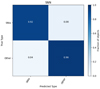 |
Fig. B.1. Confusion matrix for SNN classification for one LSST realization. |
Appendix C: Test of the likelihood method
In this section we describe the tests to check the reliability of the maximum likelihood method. Firstly, we test the method by changing the data vector (i.e. PVs). We perform different fits using the same SNe Ia but assigning different PVs. The results of these tests are shown in Figure C.1 in the case of the Spec-z sample in the redshift range 0.06 < z < 0.1, the results remain the same for all the redshift bins used in Sect. 4. The Figure shows that when we assign random PVs, with and without errors,16 the results are always compatible with zero. The results of this basic test are what we expect, since random PVs are not correlated, and hence have no information about the large-scale structure. We also run the test using the true PVs from the simulation, with and without errors. In both cases, we are always able to recover the input value for the growth-rate parameter. The results of these tests show that the maximum likelihood always behaves as expected. Figure C.1 shows also the result using PVs measured from SNe Ia from Eq.(10) for comparison.
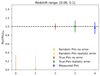 |
Fig. C.1. fσ8 results in the redshift range 0.06 < z < 0.1 for five different data vectors as defined in the legend. The colored points shows the averages over the eight LSST realizations with the average relative errors. |
Appendix D: Fit results of the Hubble diagram parameters
In this Appendix we show the fit results for the other parameters of the maximum likelihood method. We do not show the results on σu since those are prior dominated, see also Carreres et al. (2023) for detailed discussion about the prior on σu parameter.
Figure D.1 shows the fit results of the HD parameters and σv for the Full sample, Spec-z sample and Photo-typed sample in the same redshift bins as the ones used for fσ8 measurements. Figure D.1 shows that the results for α and β start to be biased as the redshift increases. A bias of ∼0.01 in α and ∼0.1 in β shifts the estimated PVs by ∼40 km/s at z = 0.1. This bias in the PVs is one order of magnitude smaller than the measurement errors at that redshift. Therefore, the bias in α and β is small and has no impact on the growth-rate measurements. The small bias in α and β results indicates the presence of Malmquist bias, as discussed in Sect. 4.1. Moreover, we notice that the mean M0 we recover in the lowest redshift bin is slightly higher than the input value, but still compatible within the error. This is the effect of PVs and is extensively discussed in Carreres et al. (2025b).
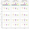 |
Fig. D.1. Result of HD parameter fits for all the scenarios in different redshift bins. Left: Full sample. Center: Spec-z sample. Right: Photo-typed sample. For each scenario, the top panel shows the results for α, then in order going down: β,M0, σM and σv. The results are shown for each of the eight LSST realizations together with the mean value. The averages are plotted at the mean redshift positions, while the results for the individual realizations are slightly shifted along the x-axis to improve the clarity of the figure. For each scenario, the black dotted line shows the value of the simulation input. The colored bars show the redshift range used for each fit, the bars have the same colors as the measurements. |
Appendix E: fσ8 forecast across the LSST years
Using the Photo-typed sample as our baseline, we produce forecasts for the expected error on the growth rate across the LSST survey years of observation. Figure E.1 shows the results of our forecast on the fσ8 uncertainty as a function of LSST years-of-observation, considering the rolling cadence, for the different redshift bins used in Sect.4. All the results shown in Fig. E.1 are the average over the eight LSST realizations. The cosmic variance limit shown in the Figure is computed using the Fisher Matrix formalism implemented in FLIP (see Ravoux et al. 2025). To compute the Fisher forecast we assume a density one million times the one shown in Fig. 4, and we fix σv = 300 km s−1, σM = 0.12 and σu = 15 h−1 Mpc. Figure E.1 shows that we have a great improvement on the precision passing from year 1 to year 5 reaching ∼20%, which is similar to the constraint from ZTF SNe Ia (19% at z < 0.06, see Carreres et al. (2023)). After 5 years of observations the precision continues to improve reaching 12% in the redshift range 0.02 < z < 0.14. We conclude that after 5 − 6 years of LSST we will be competitive in measuring the growth-rate parameter from SN Ia PVs.
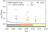 |
Fig. E.1. Error on the growth-rate parameter across the LSST duration in different redshift bins. The redshift bins are shown by the colored bars at the bottom of the figure. The points in the same redshift bin have the same color, but different sizes depending on the years. The dotted black line shows the cosmic variance limit. |
All Tables
All Figures
|
Fig. 1. LSST survey footprint showing the number of visits (Nvisits) in each sky location. The top panel shows the visits during the third year when the rolling cadence is active, and the bottom pabnel shows the survey as expected after completion (ten years of observations). |
| In the text | |
|
Fig. 2. SN-host redshift efficiencies, Rhost, as a function of redshift for each type of SN in the simulation. The top panel shows the efficiencies for DESI BGS survey, the central panel shows the ones for 4MOST CRS BG survey and the bottom panel shows the efficiencies for 4MOST 4HS surveys. The gray shaded area shows the redshift range of interest for LSST PV measurement. |
| In the text | |
|
Fig. 3. Density maps of the different SN Ia samples across the LSST footprint. SN density in the initial simulated sample (a), density of the Full sample (b), and density of the Spec-z sample (c). All the maps represent the average over the eight LSST realizations. |
| In the text | |
|
Fig. 4. Redshift distribution (top panel), comoving density (middle panel), and redshift completeness (bottom panel) for the Full and Spec-z samples. The Full sample detection and Spec-z sample detection show the results for the samples before running the SALT fit. The Full sample cosmology and Spec-z sample cosmology present the samples after the quality cuts on the SALT fit results. All the results are the average over the eight LSST realizations. The completeness distributions are computed with respect to the initial simulated sample (considering only the SNe Ia). |
| In the text | |
|
Fig. 5. Hubble diagram residuals as a function of the observed redshift (top panel) and cosmological redshift (bottom panel) for the Full sample. The solid gray lines show the residual for each of the eight LSST realizations, the red points show the mean of the eight mocks, and the blue points show the mean computed by stacking all the mocks. |
| In the text | |
|
Fig. 6. Difference between estimated PVs (vp) and true PVs (vp, true) as a function of the observed redshift for the Full sample. The solid gray lines shows the residual for each of the eight LSST realizations, the red points are the means over the eight mocks, and the blue points show the means computed by stacking all the mocks. |
| In the text | |
|
Fig. 7. Results of fσ8 measurements for all the scenarios in different redshift bins. Left: Full sample. Center: Spec-z sample. Right: Photo-typed sample. For each scenario, the top panel shows the results of the fit for each of the eight LSST realizations together with the mean value, and the bottom panel shows the mean values of σfσ8/fσ8, fid, which are the relative errors on the growth-rate measurements. The averages are plotted at the mean redshift positions, while the results for the individual realizations are slightly shifted along the abscissa for clarity. The colored bars show the redshift range used for each fσ8 measurement; the bars have the same colors as the measurements. |
| In the text | |
|
Fig. 8. HD residuals (top panel) and residuals of the estimated velocities (bottom panel), normalized by the errors, using the input HD parameters of the simulation. The plot shows the residuals for a random realization in the simulation in the redshift range 0.02 < z < 0.14. The different colors represent different SN samples with different levels of contamination, as shown in the legend. |
| In the text | |
|
Fig. 9. fσ8 fit results (top panel) and relative error (bottom panel) as a function of the sample contamination fraction for the redshift bin 0.02 < z < 0.14. The blue points show the results for the Spec-z sample, the orange points show the Photo-typed sample, and the red points show the different samples created using the cuts on the SALT fits as classification (SALT cuts). Every point is the average over the eight LSST realizations. |
| In the text | |
|
Fig. 10. Growth-rate parameter as a function of redshift. The solid black line shows the GR-ΛCDM prediction, and the gray lines present the predictions for alternative gravity theories. The points show different forecasts for future and current stage IV surveys. The orange points show the forecast for Euclid (Amendola et al. 2018), and the red circles show those for DESI (DESI Collaboration 2016). The forecasts from DESI and Euclid are derived from the analysis of the density field. The other forecasts come from the PV field: the green triangle from ZTF SNe Ia (Carreres et al. 2023), the cyan circles from the DESI PV survey (Saulder et al. 2023), and the blue crosses from LSST SNe Ia, which are the results from the Photo-typed sample in the tomographic bins. |
| In the text | |
|
Fig. B.1. Confusion matrix for SNN classification for one LSST realization. |
| In the text | |
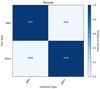 |
Fig. B.2. Confusion matrix for Parsnip classification for the same LSST realizations as Fig. B.1. |
| In the text | |
|
Fig. C.1. fσ8 results in the redshift range 0.06 < z < 0.1 for five different data vectors as defined in the legend. The colored points shows the averages over the eight LSST realizations with the average relative errors. |
| In the text | |
|
Fig. D.1. Result of HD parameter fits for all the scenarios in different redshift bins. Left: Full sample. Center: Spec-z sample. Right: Photo-typed sample. For each scenario, the top panel shows the results for α, then in order going down: β,M0, σM and σv. The results are shown for each of the eight LSST realizations together with the mean value. The averages are plotted at the mean redshift positions, while the results for the individual realizations are slightly shifted along the x-axis to improve the clarity of the figure. For each scenario, the black dotted line shows the value of the simulation input. The colored bars show the redshift range used for each fit, the bars have the same colors as the measurements. |
| In the text | |
|
Fig. E.1. Error on the growth-rate parameter across the LSST duration in different redshift bins. The redshift bins are shown by the colored bars at the bottom of the figure. The points in the same redshift bin have the same color, but different sizes depending on the years. The dotted black line shows the cosmic variance limit. |
| In the text | |
Current usage metrics show cumulative count of Article Views (full-text article views including HTML views, PDF and ePub downloads, according to the available data) and Abstracts Views on Vision4Press platform.
Data correspond to usage on the plateform after 2015. The current usage metrics is available 48-96 hours after online publication and is updated daily on week days.
Initial download of the metrics may take a while.