| Issue |
A&A
Volume 702, October 2025
|
|
|---|---|---|
| Article Number | A50 | |
| Number of page(s) | 20 | |
| Section | Extragalactic astronomy | |
| DOI | https://doi.org/10.1051/0004-6361/202452650 | |
| Published online | 06 October 2025 | |
GA-NIFS and EIGER: A merging quasar host at z = 7 with an overmassive black hole
1
Los Alamos National Laboratory, Los Alamos, NM, 87545, USA
2
MIT Kavli Institute for Astrophysics and Space Research, 77 Massachusetts Ave., Cambridge, MA, 02139, USA
3
Kavli Institute for Cosmology, University of Cambridge, Madingley Road, Cambridge, CB3 0HA, UK
4
Cavendish Laboratory – Astrophysics Group, University of Cambridge, 19 JJ Thomson Avenue, Cambridge, CB3 0HE, UK
5
Centro de Astrobiología (CAB), CSIC-INTA, Ctra. de Ajalvir km 4, Torrejón de Ardoz, E-28850 Madrid, Spain
6
National Research Council of Canada, Herzberg Astronomy & Astrophysics Research Centre, 5071 West Saanich Road, Victoria, BC, V9E 2E7, Canada
7
Department of Physics and Astronomy, University College London, Gower Street, London, WC1E 6BT, UK
8
Max-Planck-Institut für extraterrestrische Physik, Gießenbachstraße 1, 85748 Garching, Germany
9
University of Oxford, Department of Physics, Denys Wilkinson Building, Keble Road, Oxford, OX13RH, United Kingdom
10
Sorbonne Université, CNRS, UMR 7095, Institut d’Astrophysique de Paris, 98 bis bd Arago, 75014 Paris, France
11
European Space Agency, c/o STScI, 3700 San Martin Drive, Baltimore, MD, 21218, USA
12
Scuola Normale Superiore, Piazza dei Cavalieri 7, I-56126 Pisa, Italy
13
Institut de Radioastronomie Millimétrique (IRAM), 300 rue de la Piscine, 38400 Saint-Martin-d’Hères, France
14
INAF – Osservatorio Astrofisico di Arcetri, largo E. Fermi 5, 50127 Firenze, Italy
15
Department of Physics, North Carolina State University, Raleigh, NC, 27695-8202, USA
16
National Astronomical Observatory of Japan, 2-21-1 Osawa, Mitaka, Tokyo, 181-8588, Japan
17
Laboratoire d’astrophysique, Ecole Polytechnique Fédérale de Lausanne (EPFL), Observatoire, CH-1290 Versoix, Switzerland
18
Institute of Science and Technology Austria (ISTA), Am Campus 1, 3400 Klosterneuburg, Austria
⋆ Corresponding author: This email address is being protected from spambots. You need JavaScript enabled to view it.
Received:
17
October
2024
Accepted:
3
August
2025
Abstract
The James Webb Space Telescope is revolutionising our ability to understand the host galaxies and local environments of high-z quasars. Here we obtain a comprehensive understanding of the host galaxy of the z = 7.08 quasar J1120+0641 by combining NIRSpec integral field spectroscopy with NIRCam photometry of the host continuum emission. Our emission-line maps reveal that this quasar host is undergoing a merger with a bright companion galaxy. The quasar host and the companion have similar dynamical masses of ∼1010 M⊙, suggesting that this is a major galaxy interaction. Through detailed quasar subtraction and SED fitting using the NIRCam data, we obtained an estimate of the host stellar mass of M* = (3.0−1.4+2.5) × 109 M⊙, with M∗ = (2.7−0.5+0.5) × 109 M⊙ for the companion galaxy. Using the Hβ Balmer line, we estimated a virial black hole mass of MBH = (1.9−1.1+2.9) × 109 M⊙. Thus, J1120+0641 has an extreme black hole–stellar mass ratio of MBH/M* = 0.63−0.31+0.54, which is ∼3 dex larger than expected by the local scaling relations between black hole and stellar mass. J1120+0641 is powered by an overmassive black hole with the highest reported black hole–stellar mass ratio in a quasar host that is currently undergoing a major merger. These new insights highlight the power of JWST for measuring and understanding these extreme first quasars.
Key words: galaxies: high-redshift / galaxies: interactions / quasars: general / quasars: supermassive black holes
© The Authors 2025
 Open Access article, published by EDP Sciences, under the terms of the Creative Commons Attribution License (https://creativecommons.org/licenses/by/4.0), which permits unrestricted use, distribution, and reproduction in any medium, provided the original work is properly cited.
This article is published in open access under the Subscribe to Open model. This email address is being protected from spambots. You need JavaScript enabled to view it. to support open access publication.
1. Introduction
High-redshift quasars at z ≥ 6 powered by highly accreting supermassive black holes (BHs) with masses up to ∼109 M⊙ (e.g. Fan et al. 2000, 2001, 2003; Willott et al. 2009, 2010; Kashikawa et al. 2015; Bañados et al. 2016, 2018, 2022; Matsuoka et al. 2018; Wang et al. 2019; Yang et al. 2023a) are some of the most extreme objects in the Universe, and they raise serious questions about the nature of the first BH seeds and BH growth mechanisms. However, much is yet to be fully understood about these objects due to limitations in the ability to study their host galaxies, BH properties, and environments.
Prior to the launch of the James Webb Space Telescope (JWST; Gardner et al. 2006, 2023; McElwain et al. 2023), the host galaxies of these high-z quasars could only be seen in the rest-frame far-infrared (FIR), detected in the sub-millimetre with the Plateau de Bure Interferometer (PdBI; e.g. Bertoldi et al. 2003; Walter et al. 2003), later upgraded to the Northern Extended Millimetre Array (NOEMA; e.g. Bañados et al. 2015; Mazzucchelli et al. 2017), and the Atacama Large Millimeter Array (ALMA; e.g. Wang et al. 2013; Willott et al. 2013). This emission traces the cold gas and dust, allowing the host dynamical masses (1010–1011 M⊙), dust masses (107–109 M⊙), radii (∼1–5 kpc), obscured star-formation rates (SFRs; 10–2700 M⊙/yr), and their various morphologies to be measured (Walter et al. 2009; Wang et al. 2013; Venemans et al. 2015, 2017; Willott et al. 2017; Izumi et al. 2018; Pensabene et al. 2020; Neeleman et al. 2021; Salvestrini et al. 2025; Mazzucchelli et al. 2025). These observations have shown that there is a variety in high-z quasar host galaxy properties. For a more comprehensive understanding of the full picture of these host galaxies, however, observations of their stellar emission as well as other gas phase (i.e. ionised) components are required.
In the rest-frame ultraviolet (UV)–optical, where the majority of the stellar emission occurs, the bright quasar significantly outshines the host galaxy (e.g. Schmidt 1963; McLeod & Rieke 1994; Dunlop et al. 2003; Hutchings 2003; Floyd et al. 2013). At high-z, the size of the galaxies becomes small relative to the point spread function (PSF) of current telescopes, so the faint host galaxy emission is hidden underneath the bright quasar point source (e.g. Mechtley et al. 2012). Thus, to detect the host, deep imaging with sufficiently high spatial resolution to decompose the galaxy and quasar emission is required. However, even with the resolution of the Hubble Space Telescope (HST), this quasar subtraction process had been unsuccessful in obtaining any high-z host detections (Mechtley et al. 2012; Decarli et al. 2012; McGreer et al. 2014; Marshall et al. 2020).
With a spatial resolution of  at 1 μm, which is almost three times better than that of HST, JWST has provided the first rest-frame UV/optical high-z quasar host galaxy detections. Ding et al. (2023) detected the hosts of two low-luminosity (MUV ≃ −23.9 mag and −23.7 mag) quasars at z ≃ 6.4 by performing detailed PSF modelling and quasar removal from images from the Near-Infrared Camera (NIRCam; Rieke et al. 2023). Using a similar approach, Yue et al. (2024) detected the host galaxies of three of their sample of six luminous (MUV ≃ −29 to −26 mag) z ≳ 6 quasars. Stone et al. (2023) have also claimed a successful host detection of a quasar at z = 6.25. Thus, with JWST these host detections are now possible, and measurement of their stellar properties can begin.
Notably, by measuring the stellar continuum of these hosts, their stellar masses can be calculated. One key question is whether early BHs grew more efficiently than their hosts, in which case they should be comparatively more massive than their present day equivalents, and therefore they would fall above the local BH–stellar mass relation (e.g. Magorrian et al. 1998; Marconi & Hunt 2003; Häring & Rix 2004; Kormendy & Ho 2013; Reines & Volonteri 2015; Greene et al. 2020). Yue et al. (2024) measured their three quasars, finding them to have BH–stellar mass ratios of ∼0.15, 1–2 dex larger than expected from the local Reines & Volonteri (2015) and Kormendy & Ho (2013) BH–stellar mass relations; however, these BHs are overly massive, even when considering selection effects. The lower luminosity quasars presented in Ding et al. (2023) are consistent with the local BH–stellar mass relations of Häring & Rix (2004) and Bennert et al. (2011) when accounting for selection effects. Some observations of confirmed and candidate z > 3 active galactic nuclei (AGNs; not in the quasar regime) support the picture of overmassive BHs relative to the local relation (Übler et al. 2023; Harikane et al. 2023; Maiolino et al. 2024; Pacucci et al. 2023). However, Sun et al. (2025) found no evidence of the evolution of the BH–stellar mass relation up to z ≃ 4. Selection effects, measurement uncertainties, and low sample sizes make a redshift evolution of the BH–stellar mass relation difficult to confirm (Li et al. 2025).
Another key piece of this puzzle is obtaining accurate measurements of BH masses. Prior to JWST, all high-z quasar BH mass estimates relied on the Mg II and C IV emission lines. However, Mg II- and C IV-based reverberation mapping calibrations are more uncertain than those based on the broad hydrogen lines (e.g. Trevese et al. 2014; Kaspi et al. 2021) and therefore give less reliable single-epoch BH mass estimates (e.g. Shen et al. 2008; Shen & Kelly 2012; Peterson 2009; Coatman et al. 2016; Farina et al. 2022). The hydrogen lines from the quasar’s broad-line region (BLR) have previously been unobservable beyond z ≳ 4. With JWST, Hβ is now observable up to z = 9.8 and Hα up to z = 7.0 with the Near-Infrared Spectrograph (NIRSpec; Jakobsen et al. 2022; Böker et al. 2023) and to even higher redshifts with the Mid-Infrared Instrument (MIRI; Rieke et al. 2015). This allows us to determine the BH masses of these quasars more accurately (e.g. Eilers et al. 2023; Yang et al. 2023b; Marshall et al. 2023) and to obtain a clearer understanding of the BH growth history and ongoing accretion.
Alongside measuring the quasar host properties, for a full picture of this rapid early BH growth, we must understand their environments. Some theories have suggested that intense BH growth can be caused via galaxy–galaxy mergers and local kiloparsec-scale interactions (e.g. Sanders et al. 1988; Hopkins et al. 2006), which may be more prevalent in the early Universe. Mergers are also suggested to be a potential cause of the observed BH–host scaling relations (e.g. Di Matteo et al. 2005; Croton 2006). ALMA has uncovered major galaxy interactions around high-z quasars at rates of up to 50% (Trakhtenbrot et al. 2017), with companions found at ≃8–60 kpc separations (e.g. Wagg et al. 2012; Decarli et al. 2017; Venemans et al. 2020). These companions have been less frequently detected in the rest-frame UV (Willott et al. 2005), likely due to their dusty nature (Trakhtenbrot et al. 2017). With spatially resolved spectroscopic capabilities and coverage in the rest-frame optical where dust is less prevalent, JWST has the power to uncover the local environments of high-z quasars in greater detail than ever reported before.
The NIRSpec Integral Field Unit (IFU; Böker et al. 2022) can reveal detailed kinematics around quasars on the kiloparsec-scale (e.g. Perna et al. 2023; Marshall et al. 2023). Marshall et al. (2023) studied two z = 6.8 quasars and discovered three kiloparsec-scale companion galaxies; one companion is merging with one of the quasars, while two are merging with the other. The quasar–galaxy merger PJ308–21 at z ≃ 6.2 discovered with ALMA (Decarli et al. 2019) has been observed with the NIRSpec IFU to study the ionised gas and stellar emission (Loiacono et al. 2024) and the interplay of gas, dust, star formation, and nuclear activity (Decarli et al. 2024). Perna et al. (2023) used the IFU to investigate a quasar at z = 3.3 that lives in an extreme environment with multiple companion galaxies and found that one of these companions is hosting an obscured AGN. At z = 7.15, Übler et al. (2024) discovered an AGN within a galaxy–galaxy merger, with two BHs expected to merge in the future. After detailed quasar subtraction, NIRCam images from Yue et al. (2024) also revealed extended emission structures, companion galaxies, and/or potential merger signatures around the majority of their six z ≳ 6 quasars. NIRSpec IFU and NIRCam imaging of an AGN at z = 5.55 showed that the AGN has two faint nearby companions (Übler et al. 2023; Ji et al. 2024). The z = 8.7 AGN of Larson et al. (2023) appears asymmetric in their NIRCam images, with companion galaxies that imply a major merger. Matthee et al. (2024) found that around the faint (MUV ≃ −20 to −17 mag) AGNs at z ≃ 4–6 discovered with the NIRCam, the majority show at least one spatially separated companion, while similar AGNs in Maiolino et al. (2024) show evidence of two broad components of Hα, which they suggest could be signatures of merging BHs. Perna et al. (2025) found that companions are routinely observed around AGNs at 3 < z < 6 within a radius of ∼10 kpc and that a significant fraction of them could host accreting BHs. Thus, while companion galaxies are not observed around all high-z quasars, these observations support the picture of major mergers being potential drivers of rapid early BH growth.
At z = 7.08, ULAS J112001.48+064124.3 (hereafter J1120+0641) was the first quasar discovered at z > 7 (Mortlock et al. 2011). This was the highest-z quasar known until the 2018 discovery of ULAS J134208.10+092838.61, at z = 7.54 (Bañados et al. 2018), and it remains the fourth highest-z quasar known to date (after Yang et al. 2020; Wang et al. 2021), thus making it one of the most targeted high-z quasars with JWST so far. As part of the Emission-line galaxies and Intergalactic Gas in the Epoch of Reionization (EIGER) project, J1120+0641 was observed with the NIRCam with deep F115W, F200W, and F356W imaging and slitless F356W grism spectroscopy (Yue et al. 2024). J1120+0641 was also imaged with the NIRCam F210M, F360M, and F480M filters (Stone et al. 2024). Bosman et al. (2024) observed J1120+0641 with the MIRI Medium-Resolution Spectrometer (MRS), obtaining IFU spectra from 4.9–27.9 μm. These observations have led to two key results. Firstly, Yue et al. (2024) detected the stellar emission from the host of J1120+0641, providing the first stellar mass measurement of  . Secondly, with measurements of the broad hydrogen lines, we can be more confident in the BH mass estimates. Yue et al. (2024) measured MBH = (1.19 ± 0.08)×109 M⊙ from Hβ, and Bosman et al. (2024) measured MBH = (1.55 ± 0.22)×109 M⊙ from Hα. Accounting for the estimated 0.43 dex scatter in the hydrogen-based BH mass scaling relations (Vestergaard & Peterson 2006), these estimates become
  from Hβ and
  from Hα. With a BH mass of ∼10–25% of the stellar mass estimate, these measurements imply that J1120+0641 lies significantly above the local BH–host mass relation, which predicts ratios of only ∼0.1% (Greene et al. 2020).
Within the Galaxy Assembly with NIRSpec Integral Field Spectroscopy (GA-NIFS) programme, J1120+0641 was observed with the NIRSpec IFU, obtaining high-resolution (R ∼ 2700) spectra from 2.9–5.3 μm across the 3′′ × 3′′ field of view (FOV). In this paper, we present the GA-NIFS IFU data for J1120+0641, showing the detailed emission-line structures around the quasar. By combining this spatially resolved emission-line data with the detailed photometry from the EIGER NIRCam imaging, we are able to gain a much clearer picture of this system, discovering that it is undergoing a major merger with a companion galaxy and estimating the quasar host stellar mass more accurately. This paper is organised as follows. We discuss the observations, our data reduction, and analysis techniques in Section 2. In Section 3 we show the results from the NIRSpec IFU data, including the emission-line structure and kinematics, dynamical mass estimates, and BH mass measurements. In Section 4 we show updated results from the NIRCam data, including the resulting spectral energy distribution (SED) fitting when combining both the NIRSpec IFU and NIRCam imaging. We include a discussion in Section 5 and conclude in Section 6.
Throughout this work we adopt the WMAP9 cosmology (Hinshaw et al. 2013) as included in ASTROPY (Astropy Collaboration 2013), with H0 = 69.32 km /(Mpc s), Ωm = 0.2865, and ΩΛ = 0.7134. All magnitudes are on the AB system.
2. Observations and data analysis
2.1. NIRSpec IFU data reduction and analysis
For our NIRSpec IFU data, we follow the same reduction and analysis procedure as in Marshall et al. (2023), with several updates. Here we give an overview, but refer the reader to Marshall et al. (2023) for full details. To summarise our data analysis, once we have reduced the data, we first perform background and continuum subtraction. We then remove the point-source quasar line emission from the data cube via detailed PSF modelling. Using this quasar-subtracted cube we make Hβ and [O III] λλ4959,5007 emission-line maps to study the extended host kinematics. We separately integrate the original continuum-subtracted cube to obtain a quasar spectrum, which we fit with a detailed model in order to measure the BH mass.
2.1.1. NIRSpec IFU observations
The quasar J1120+0641 was observed as part of the GA-NIFS Guaranteed Time Observations (GTO) programme1. In order to save overhead time, the NIRSpec observations were combined with those using MIRI in programme #1263 (PI L. Colina). It was observed with the NIRSpec IFU, which provides spectroscopy over a 3″ × 3″ FOV in each of the  spatial elements, with a grating/filter pair of G395H/F290LP, giving a spectral resolution of R ∼ 2700 over the wavelength range 2.87–5.27 μm. The observations were taken with a NRSIRS2 readout pattern (Rauscher et al. 2017) with 25 groups per integration and one integration per exposure, using a 6-point medium cycling dither pattern, with a total on-source exposure time of 11 029 seconds.
J1120+0641 was observed on December 11, 2022, at a position angle (PA) of 70.97 degrees. We constrained the allowable PA window to minimise the leakage of light through the micro-shutter assembly (MSA) from bright sources. We also offset the quasar within the detector by  from the centre to ‘mind the gap’. The physical gap between the two NIRSpec detectors results in a range of unobservable wavelengths from ∼4.0–4.2 μm which varies with IFU slice (Böker et al. 2022). At this redshift, the quasar’s [O III] λλ4959,5007 fall around this detector gap, and so offsetting the quasar within the detector allowed these lines to be observed.
2.1.2. IFU data reduction
The IFU data was reduced with the JWST calibration pipeline version 1.8.2 (Bushouse et al. 2022), using the context file JWST_1068.PMAP. We applied additional corrections to improve the data quality: correcting the count-rate frames such that the background base-level is consistent with zero counts per second; subtracting the 1/f noise (Moseley et al. 2010), by modelling and then subtracting it from each column (i.e. along the spatial axis); and implementing a modified version of the LACOSMIC algorithm (van Dokkum 2001) in the JWST pipeline for outlier detection (details in D’Eugenio et al. 2024); full details of the data reduction process can be found in Perna et al. (2023).
In this work we used the CUBE_BUILD step in the pipeline to produce combined data from the various dithers. We created 0.05″/pixel cubes using the ‘drizzle’ weighting–this optimises the spatial resolution of the data. However, these cubes are affected by oscillations in the extracted spectra due to re-sampling effects (see Law et al. 2023; Perna et al. 2023). These oscillations (or ‘wiggles’) impact the accurate determination of the continuum and emission-line profiles at the spaxel level, which is crucial for both PSF modelling and subtraction, and consequently, for studying the quasar host galaxy. To address this, we applied the same method detailed in Perna et al. (2023), and subtracted the wiggles in each individual spaxel in the close surroundings of the quasar. The resulting integrated (background-subtracted) spectrum for J1120+0641 is shown in Figure 1, showing the full wavelength coverage from 2.87–5.27 μm, corresponding to rest-frame 3550–6520 Å at z = 7.085.
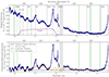 |
Fig. 1. Integrated spectrum of J1120+0641 from the IFU data (blue). The spectrum is integrated over an aperture of radius |

The noise estimation from the ‘ERR’ cube produced by the pipeline underestimates the actual noise in the data. We therefore rescaled the ERR cube to match the noise estimated from the continuum emission (as in e.g. Übler et al. 2023; Rodríguez Del Pino et al. 2024; Jones et al. 2024; Lamperti et al. 2024). For each spaxel we measured the root mean square (RMS) noise across 3.78–3.83 μm, just blueward of Hβ, and compare this to the mean ERR value across the same region. In spaxels where the ratio of RMS to the mean ERR is greater than 1, we multiplied the ERR spectrum by this fraction. This results in a final error spectrum that is a median of 50% larger than the original ERR array. However, we note that because of the uncertainty introduced via the wiggle subtraction, continuum subtraction, and various interpolations/re-samplings (i.e. smoothing the data), this will also be an under-estimate of the true noise.
Due to an uncertainty in the specified astrometry of our IFU observations, we astrometrically aligned our IFU data to the EIGER data. We integrated our cube across the wavelength range covered by the F356W filter, and matched the quasar location in the resulting image to that in the EIGER F356W image, which has been aligned to the Gaia DR2 catalogue (Gaia Collaboration 2018) with the quasar located at RA 11:20:1.464, Dec +6.41.23.783. In Figure 2 we show this quasar peak from the NIRCam data compared to the peak of the 158 μm FIR continuum emission from ALMA and the quasar position from its discovery with the UK Infrared Telescope (UKIRT) Infrared Deep Sky Survey (UKIDSS). In the ALMA study of Venemans et al. (2017), the FIR continuum emission was found to peak at RA 11:20:01.465; Dec +06:41:23.810, offset  to the south-west of the quoted quasar position from UKIDSS (Mortlock et al. 2011), RA 11:20:01.480; Dec +06:41:24.300. From the NIRCam imaging, the quasar location is consistent with the ALMA location, also offset from the UKIDSS location. UKIDSS is astrometrically aligned to 2MASS, with an astrometric accuracy of 0
 1 (Lawrence et al. 2007). The UKIDSS images have a pixel scale of 0
 4 (Lawrence et al. 2007), and so the coarse spatial resolution may also contribute to the large astrometric offset. ALMA is astrometrically aligned with the International Celestial Reference Frame to an accuracy of
  ; the astrometry of individual sources depends on frequency, baseline, and signal-to-noise ratio S/N, which for this target results in an expected position uncertainty of
  (ALMA Cycle 7 Technical Handbook2). The NIRCam images are aligned to Gaia DR2, with accuracy of 0
 0015 (Anderson et al. 2021). We conclude that the higher spatial resolution and more accurately aligned NIRCam and ALMA images give a more accurate position of the quasar, with the original UKIDSS quasar position offset 0
 5 to the north-east from its true location.
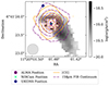 |
Fig. 2. Quasar-subtracted [O III] λ5007 emission map from the NIRSpec IFU (grey image) compared to the [C II] 158 μm emission map (orange contours) and the rest-frame 158 μm FIR continuum emission map (purple contours) from ALMA (see Section 5.2). The [C II] 158 μm contours are linearly spaced from 5σ to 26σ, where σ = 16 μJy. The FIR continuum contours are linearly spaced from 5σ to 42σ, where σ = 7 μJy/beam. The grey circle depicts the approximate PSF of the ALMA observations, with beam diameter |

2.1.3. Background and continuum subtraction
For our analysis, we first subtracted the background and continuum emission from our quasar cube in each spaxel. We selected a background region with circular aperture of radius 0 25 near a corner of the IFU FOV chosen to avoid the PSF of the quasar and the extended emission as well as the higher-noise pixels around the edge of the FOV. We measured the median spectrum across spaxels within this aperture and fit this spectrum with a polynomial function of fourth order. We then subtracted this polynomial curve from each spaxel to subtract the background.
For the continuum subtraction, we considered the flux in the emission-line- and iron-continuum-free windows at rest-frame 3790–3800 Å, 4200–4220 Å, 5630–5650 Å, and 5970–6000 Å, following Kuraszkiewicz et al. (2002) and Kovacevic et al. (2010), as well as additional windows near the blue and red edges of the spectral range at 3680–3700 Å and 6260–6280 Å to better constrain the continuum across the full wavelength range. For each spaxel we measured the S/N across these continuum windows and modelled and subtracted the continuum if the median S/N ≥ 1.5. We find that spaxels with median S/N < 1.5 across their continuum windows have negligible contribution to the continuum in the final integrated spectra. For spaxels with median S/N ≥ 1.5 in the continuum windows, we measured the mean flux and wavelength in each continuum window and interpolated between these means with SCIPY’s INTERP1D function using a spline interpolation of second order. We evaluated the interpolation function across the full wavelength range, producing a full continuum model in each spaxel that was then subtracted from the spectrum. Each spaxel was modelled independently, and this created a continuum-subtracted data cube. Figure 1 shows the quasar spectrum as integrated from the original cube as well as from the continuum-subtracted cube, for comparison. Throughout the remainder of this work, we only use the continuum-subtracted cube.
2.1.4. IFU quasar subtraction
To study the extended narrow-line emission from the host galaxy system, we must first subtract the quasar’s large contribution to the emission. The narrow-line emission can be emitted both by the quasar, photoionised by the AGN and shocks, and gas throughout the system that has been photoionised by star formation. We remove the bright unresolved narrow-line emission from the nucleus to study the spatial distribution and kinematics of the extended host system. The quasar BLR is spatially unresolved, and so its emission traces the PSF of the instrument; we use this fact to perform our quasar subtraction.
Step 1, Measuring the spatial PSF: We used QDeblend3D (Husemann et al. 2013, 2014), which uses the relative strength of quasar broad lines in each spaxel to determine the spatial PSF shape. After continuum subtraction (Section 2.1.3), in each spaxel we measured the mean of the broad-line flux between rest-frame 4800–4830 Å and 4880–4910 Å, on both sides of the peak of Hβ. These spectral windows cover the broad-line wings, and are free from any narrow lines that would bias the measurement. These broad-line wing fluxes were normalised to that of the central brightest quasar spaxel, giving the 2D PSF.
For our final PSF shape, we selected spaxels in which the S/N > 10 for at least three consecutive sampled wavelengths within the broad-line region, and then expanded this region spatially by selecting any adjacent spaxels with S/N > 2 at two consecutive wavelengths, following the FIND_SIGNAL_IN_CUBE algorithm of Sun (2020) (see also Sun et al. 2018). To reduce the effect of any artefacts and companion galaxies on the measured PSF shape, we then excluded any spaxels that are located more than 10σ from the quasar peak, where  and the full width at half maximum (FWHM) is the diffraction limit of the telescope at the observed wavelength of Hβ,
  . Our measured spatial PSF is shown in Figure A.1.
Step 2, Creating a 3D quasar model cube: For our 1D quasar spectral model, we used the spectrum of the brightest spaxel, the centre of the quasar emission, under the assumption that the host line emission in that spaxel is negligible relative to the dominant quasar emission. This spectrum includes both the narrow and broad-line quasar emission, and so both the unresolved quasar narrow and broad emission is subtracted. We created a 3D quasar cube by scaling the quasar spectrum by the 2D PSF, and subtracted this from our original continuum-subtracted cube to create our host galaxy cube. We are able to ignore the variation of the PSF with wavelength, because we only analyse the Hβ and nearby [O III] λλ4959,5007 lines.
To account for the additional uncertainty associated with the quasar subtraction, we created a new error cube (see Marshall et al. 2023, for more details). We generated 200 realisations of the continuum-subtracted cube with normally distributed noise, taken from the original noise cube. We then performed the quasar subtraction on each of the realisations. In each spaxel, we measured the standard deviation across the 200 realisations at each wavelength both before and after quasar subtraction. We then measured the mean standard deviation across the rest-frame 50 Å surrounding Hβ before and after quasar subtraction, σoriginal and σquasar subtracted. We multiplied the original noise cube by σquasar subtracted/σoriginal, in spaxels where σquasar subtracted > σoriginal; this results in a maximum increase of a factor of 2×.
2.1.5. Emission-line fitting for galaxy line maps
To create maps of the galaxy’s spatially resolved Hβ and [O III] λλ4959,5007 emission from the quasar-subtracted cube, we fit each spectrum as a series of Gaussians, with ASTROPY’S Levenberg-Marquardt algorithm. We fit the three narrow lines each as a single Gaussian, with their mean velocity and line widths constrained to be equal in velocity space, as we assume they arise from the same physical region with the same kinematics. We tied the [O III] λλ4959,5007 amplitudes to have the standard ratio of 1:2.98 (Storey & Zeippen 2000). The resulting line flux is taken to be the integrated Gaussian model. Our velocity maps show the median velocity v50, a non-parametric measure for the line centre, and the velocity dispersion w80, the width containing 80% of the line flux. The velocity dispersion maps are derived after removing the instrumental width in quadrature at each spaxel, where for NIRSpec in the G395H/F290LP configuration, the instrumental FWHM at Hβ is approximately 115 km/s at this redshift (Jakobsen et al. 2022).
Our [O III] λλ4959,5007 line maps include only spaxels with S/N > 10, and any subsequently adjacent spaxels with S/N > 1.5, following the FIND_SIGNAL_IN_CUBE algorithm of Sun (2020). Given the much lower S/N for Hβ, we included spaxels with S/N > 2, and any subsequently adjacent spaxels with S/N > 1; this Hβ flux map is only shown for visual reference and not used to infer any properties about the quasar system. For these measured line maps, we also need to exclude heavily corrupted spaxels caused by the quasar subtraction, with spaxels in which the quasar flux significantly dominated over the host galaxy having significant noise and artefacts. We therefore excluded the central 5 × 5 spaxels surrounding the quasar peak. We find an additional region of corrupted spaxels to the south-east of the quasar, within ≃7 spaxels of the peak. We find that in this region fits to the spurious spectra result in [O III] λ5007 velocity offset greater than 300 km/s from the quasar redshift, which are not seen throughout the rest of the quasar-subtracted cube. Thus, we also excluded spaxels with an [O III] λ5007 velocity offset greater than 300 km/s to excluded this region of significant contamination. The resulting quasar-subtracted emission-line maps are presented in Figure 3.
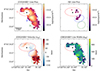 |
Fig. 3. Emission-line regions surrounding J1120+0641 showing flux and kinematic maps after the subtraction of the quasar emission. The top-left and -right panels show the flux of the [O III] λ5007 and Hβ lines, respectively, from the integrated flux of the fitted Gaussian in each spaxel. The bottom-left and -right panels show our [O III] λ5007 kinematic maps, depicting the non-parametric central velocity of the line (v50) relative to the quasar host redshift of z = 7.0804 ± 0.0028 and the line width (w80), respectively. Three emission-line regions are highlighted by coloured ellipses, and the crosses show the location of the quasar. |
2.1.6. Integrated emission-line fitting for quasar properties
To create an integrated quasar spectrum and fit a model, we used the Markov chain Monte Carlo (MCMC)-based technique of QUBESPEC3. First, we chose to integrate the continuum-subtracted data cube spatially across an aperture with radius  , centred on the peak of the quasar emission. This was chosen to maximise our S/N while containing the majority of the quasar flux, by containing the main core of the PSF, yet not including the ring of reduced flux that occurs prior to the second radial PSF peak (see Figure A.1). In Marshall et al. (2023) we found that for two quasars, the average fraction of the quasar flux contained within a
  radius aperture was 81.4% at similar wavelengths; we corrected our aperture flux by this same correction factor of 1.23× to maintain consistency.
With QubeSpec, we then fit this integrated spectrum around the Hβ line. The [O III] λλ4959,5007 lines are fit with two Gaussian components: one narrow ‘galaxy’ component, and one broader component from ionised galactic outflows. The Hβ line was also allowed to have both a narrow and outflow component; in our model the narrow and outflow components were tied to have the same redshift and line width across all three [O III] λλ4959,5007 and Hβ emission lines, as we assumed they arise from the same physical region with the same kinematics. While outflows are typically blue-shifted, we did not constrain this to be the case in our fit and allowed the narrow and outflow component fits to be completely independent. We constrained the amplitude of [O III] λ4959 to be 2.98 times less than that of [O III] λ5007 (Storey & Zeippen 2000) for both components.
For the Hβ BLR line component, we considered two separate models. For our first model, we followed the method of Marshall et al. (2023) by fitting the broad Hβ line as a broken power law (BPL) model:
 (1)
(1)
convolved with a Gaussian with standard deviation σ (as in e.g. Nagao et al. 2006; Cresci et al. 2015). Marshall et al. (2023) found that this model provided a better fit to the BLR signal of VDES J0020−3653 and DELS J0411−0907 than a single Gaussian, and so we used this BPL model for consistency. However, Yue et al. (2024) chose to fit their NIRCam grism Hβ spectroscopy of J1120+0641 with two Gaussian components, as did Bosman et al. (2024) for their MIRI spectrum. Thus, to provide a clearer comparison to these studies, we also included a model where the Hβ BLR is fit as two independent Gaussian components.
Finally, we also included a model for the iron emission blends by using templates from Boroson & Green (1992), Véron-Cetty et al. (2004), and Park et al. (2022). To choose a best-fitting iron model, we used QubeSpec to fit the integrated spectrum in the iron emission regions of rest-frame 4450–4650 Å and 5350–5600 Å with each of the different templates. We find that the Park et al. (2022) model provides the best fit to the spectrum in the main iron-continuum windows surrounding Hβ, at rest-frame ∼4400–4700 Å and ∼5200–5600 Å, with the other two models having a template shape that provides a much poorer match to the observed spectrum (see Park et al. 2022, for a comparison of the templates). Therefore, we chose to use this Park et al. (2022) iron template in our final model. We used the values of the peak flux and FWHM parameters from this Park et al. (2022) iron-only MCMC fit as constraints in the full fit to reduce the range of the free parameters. The iron emission was constrained to have the same velocity offset as the Hβ BLR in the full fit.
We ran our QubeSpec MCMC for 20 000 iterations. We have one model with a double Gaussian (DB) Hβ BLR and one model with a BPL Hβ BLR. We include results from these two similarly performing models in this work to show how the choice of model impacts the measured BH properties.
In this fitting of the integrated quasar spectrum, we measure the quasar [O III] λ5007 line to have a redshift of z = 7.0790 ± 0.0004, and the Hβ BLR component to have a redshift of z = 7.0949 ± 0.0002. We find that the [O III] λ5007 line from the integrated host galaxy spectrum, with the quasar removed, peaks at z = 7.0804 ± 0.0028. In the discovery spectrum, Mortlock et al. (2011) measured a redshift of z = 7.085 ± 0.003 from Si III], C III] and Mg II. From the ALMA [C II] 158 μm measurements of Venemans et al. (2017), the redshift is measured to be z = 7.0851 ± 0.0005. Bosman et al. (2024) measure a similar variety of redshifts depending on the specific emission line, with z = 7.092 ± 0.002 from Hα,  from Pa-α, z = 7.098 ± 0.003 from Pa-β,
  from Pa-δ, and z = 7.111 ± 0.003 from O I, excluding their estimates from blended lines. Because of this variation in redshift estimates, throughout this work we use the host galaxy [O III] λ5007 redshift of z = 7.0804 ± 0.0028 when we quote velocities and create our velocity maps.
2.2. NIRCam imaging
The NIRCam imaging of J1120+0641 used in this work was taken as part of the Emission-line galaxies and Intergalactic Gas in the Epoch of Reionization (EIGER) project (Proposal ID: 1243, PI: Lilly). We use the reduced NIRCam images of the quasar provided by Yue et al. (2024). The corresponding observations and data reduction have been described in Kashino et al. (2023), Matthee et al. (2023), Eilers et al. (2023) and Yue et al. (2024), which we briefly summarise here.
The EIGER observations of J1120+0641 contain four individual visits, which deliver NIRCam imaging in the F115W, F200W, and F356W bands, forming a 3′×6′ mosaic around the quasar. The quasar is covered by all of the four visits. Each visit consists of three dither positions following the INTRAMODULEX primary dither pattern. The exposure time per visit is 4381 s for the F115W imaging, 5959 s for the F200W imaging, and 1578 s for the F356W imaging.
The imaging data were reduced using the jwst pipeline version 1.8.4. We first ran Detector1Pipeline to generate the rate files, then ran Image2Pipeline to obtain calibrated images. For astrometry, we first aligned the calibrated images to each other using tweakwcs, then combined all the images and calibrate the absolute astrometry to the Gaia DR2 catalogue (Gaia Collaboration 2018). We corrected for 1/f noise, masked snowballs, subtracted the wisp patterns, and removed cosmic rays from the images using custom codes. We then ran Image3Pipeline to stack images within the same visit and the same module. We used a pixel size of  for the F356W images and
  for the F115W and the F200W images, which keep super-Nyquist sampling of the PSF (e.g. Zhuang & Shen 2024). The final product of the image reduction includes twelve images, corresponding to three filters and four visits.
In addition to the quasar images, we also used the NIRCam PSF models provided by Yue et al. (2024) (see their Figure 1). The PSF models were constructed using images of bright stars in EIGER observations. Yue et al. (2024) also provided the error maps of the PSF models, which reflect the spatial and temporal variations of the PSFs.
The NIRCam quasar images, PSFs, and PSF errors are used to perform quasar subtraction and reveal the quasar host emission in broad bands via image fitting in Section 4. We do this by fitting the NIRCam images with a point source (for the quasar) and two Sérsic profile models (one for the quasar host and one for the companion galaxy), using the MCMC-based technique of PSFMC (Mechtley et al. 2016), a 2D surface brightness modelling software designed for quasar–host decomposition. The detailed methods and results are described in Section 4.1.
Stone et al. (2023) reported NIRCam imaging for J1120+0641 in the F210M, F360M, and F480M bands, as part of the GTO program #1205. However, Stone et al. (2023) did not detect the host galaxy component of J1120+0641 in these bands, likely due to the limited depth of their observations. For this reason, we do not include the NIRCam images from Stone et al. (2023) in this work.
3. Spectral properties from the IFU
3.1. Emission-line structure and kinematics
In Figure 3 we present the quasar-subtracted [O III] λ5007 flux map of the J1120+0641 field. This shows two distinct peaks in the flux distribution, corresponding to the host galaxy Region 1, and a second emission-line structure Region 2 to the south-west of the quasar. There is also a much smaller and fainter region of flux further to the south-west, Region 3. This appears to have an asymmetric morphology, with a velocity that extends to higher velocities beyond the southern edge of Region 2. We define each of these three regions by elliptical apertures as shown in Figure 3. These apertures, with radius 0 2–0
2–0 5, are selected based on visual inspection of the [O III] λ5007 flux map to approximately encompass the S/N > 1.5 [O III] λ5007 flux. The edge between the Region 1 and 2 apertures is chosen to lie along the line of decreased flux between the two peaks, while the edge between Regions 2 and 3 is chosen to be where the velocity gradient in Region 2 transitions to an area of roughly constant velocity.
Based on the [O III] λ5007 map, Regions 1 and 2 are most likely two distinct galaxies. The flux in Region 1 is centrally concentrated around the quasar location (albeit corrupted by the quasar in the core). The flux in Region 2 peaks ∼0 42 to the south-west of the quasar, with a generally smooth flux profile decreasing radially from the peak. There is a noticeable decrease in [O III] λ5007 flux between these two peaks–Regions 1 and 2 are two physically distinct emission-line regions, albeit with very small spatial and velocity offset. Region 2 shows a smooth [O III] λ5007 velocity profile, from a negative velocity offset on the north-eastern edge to a positive velocity offset on the south-western edge. This indicates that Region 2 is a rotational structure. Region 2 is also clearly detected in NIRCam photometry in the F115W, F200W, and F356W filters (see Section 4.1) and thus must have moderate stellar continuum emission in the rest-frame UV–optical. This is not consistent with the properties of off-galaxy ‘Hα blobs’, clumps of gas with significant emission-line fluxes but weak or undetected optical continuum (Pan et al. 2020; Ji et al. 2021). The presence of stellar continuum, low offset velocities and line widths (Table 1), and the smooth flux and velocity structure are generally inconsistent with Region 2 being a clump of gas ejected or ionised by the central quasar. It also has significant line flux and physical size, comparable to that of the host galaxy, and so Region 2 is most likely to be a separate companion galaxy rather than a sub-clump of the host galaxy. We thus conclude that Region 2 is a companion galaxy near the quasar host. Further to the south-west, Region 3 may be a tail of extended gas emanating from Region 2, or it could be a second companion galaxy. Its irregular morphology may be physical, caused by the galaxy–galaxy interaction, or due to a lack of S/N in our observations for this faint region–deeper observations would be required to determine its physical nature.
We spatially integrated the spectra within the ellipses covering these regions, which are shown in Figure 4. These three regions are clearly at a very similar redshift to the quasar, as the doublet [O III] λλ4959,5007 lines are detected in all of the regions. We applied the same line fitting method to these integrated region spectra as we did for the individual spaxels in Section 2.1.5. The measured line properties are given in Table 1. In Figure 3 we also present the Hβ flux map, as well as a map of the [O III] λ5007 velocity v50 and velocity dispersion w80.
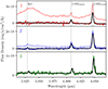 |
Fig. 4. Quasar-subtracted spectra integrated over the three spatial regions shown in Figure 3 (opaque coloured lines) along with our best-fit Gaussian models for the Hβ and [O III] λλ4959,5007 emission lines (black). The analogous spectra from the non-quasar-subtracted cube are also plotted for comparison (transparent coloured lines), showing the necessity of quasar subtraction to accurately measure the emission from Regions 1 and 2. All spectra have been continuum subtracted. The vertical lines mark the location of the Hβ and [O III] λλ4959,5007 lines at the redshift of the quasar host galaxy, Region 1, as measured from the fit to this spectrum, z = 7.0804 ± 0.0028. For the host Region 1, we exclude the central 5 × 5 pixels surrounding the quasar peak as well as nearby spaxels with [O III] λ5007 velocity offset > 300 km/s, as these are highly corrupted by the quasar subtraction and introduce significant noise and artefacts. This means that we slightly underestimate the total flux in this region; however, the fluxes are significantly more reliable than if these most corrupted spaxels were included. |
The host galaxy, Region 1, has the core region surrounding the quasar missing in the emission-line maps, with no narrow flux seen in this region of the quasar subtracted data cube. This is because the quasar subtraction technique is not capable of accurately recovering any host flux in this region, underneath the bright and dominant quasar. Realistically, the host galaxy will have narrow-line emission within this region, and so our integrated flux will underestimate the total flux due to this missing contaminated region. Inferring properties of the host is thus difficult due to this contamination. We measure that the quasar host is elongated in the east–west direction, extending across ∼1′′, where 1′′ corresponds to 5.33 kpc at z = 7.085, with the quasar located approximately in the middle along this axis. The velocity dispersion for the host from the integrated spectrum is measured to be 92 ± 49 km/s. To best estimate the properties of the host galaxy, we fit the [O III] λ5007 emission-line map with a Sérsic profile model with psfMC, using our IFU PSF estimate from our quasar subtraction as the PSF model. The best-fit Sérsic model for the host galaxy has effective radius  , axis ratio b/a = 0.41 ± 0.01, and position angle PA = 77.5 ± 0.6 deg defined counter-clockwise from north. We fixed the Sérsic index to be n = 1, as this parameter can only be poorly constrained in this difficult PSF subtraction process (see e.g. Ding et al. 2023; Yue et al. 2024).
We also fit a Sérsic model to the close companion galaxy Region 2. The best-fit Sérsic profile to the [O III] λ5007 emission of the companion galaxy with fixed n = 1 has  , b/a = 0.42 ± 0.01, and PA = 35.4 ± 0.5 deg, with the peak offset 0
 2355 or 1.25 kpc to the west and 0
 415 or 2.2 kpc to the south of the quasar host peak. The velocity map in Figure 3 clearly shows a velocity gradient across the companion, with the side closest to the quasar blueshifted relative to the far side with velocity difference ∼100 km/s. From the fit to the integrated region spectrum (Figure 4), the companion has a negligible velocity offset of only 32 ± 49 km/s from the quasar host, and a similar velocity dispersion of 104 ± 49 km/s. With this similar velocity, and the 2D sky offset of only 0
 477 corresponding to 2.5 kpc, this companion very easily satisfies the common merger criterion of having a projected distance of < 20/h kpc, where h is the dimensionless Hubble constant h = H0/(100 km/s/Mpc), and a velocity difference ΔV < 500 km/s (e.g. Patton et al. 2000; Conselice et al. 2009). The companion galaxy is measured to have very similar [O III] λλ4959,5007 and Hβ flux as the host galaxy (see Table 1)–quantifying this flux ratio more precisely is difficult due to the missing flux from the quasar core.
The third emission region directly to the south of Region 2 is four times fainter than the host and main companion, and it does not have a clear regular shape. The velocity is offset by 145 ± 49 km/s from the host galaxy, with a similarly narrow line width of 83 ± 49 km/s. As seen from the [O III] λ5007 velocity map in Figure 3, in the 2D plane of the sky this region extends spatially beyond the redshifted edge of the companion galaxy, and it has a velocity that extends gradually larger than that of the edge of the companion. This third region may be a tail of gas extending from the main companion or a third companiongalaxy.
To understand the excitation mechanisms, we considered the flux ratios of the narrow emission lines. From Table 1, the [O III] λ5007/Hβ flux ratio is 16.4 ± 4.6 for the main companion galaxy, with a limit of > 3.4 and > 7.0 for Regions 1 and 3 where Hβ was not detected. These cannot be easily classified using the traditional BPT diagram (Baldwin et al. 1981) with the existing data. Our spectra do not cover the Hα and [N II] λ6583 lines. With the spectral resolution of the MIRI data, the narrow Hα line could not be decomposed from the broad component, and [N II] λ6583 was not detected (Bosman et al. 2024). In Appendix B we plot the BPT diagram for the three regions, with horizontal ranges showing their [O III] λ5007/Hβ flux ratios. With such a high [O III] λ5007/Hβ ratio, the companion galaxy and Region 3 are likely photoionised by an AGN, lying above both the Kewley et al. (2001) and Kauffmann et al. (2003) demarcation curves. We saw no evidence of additional broad lines nor a separate point source out to ≲5.3 μm (≲6500 Å rest-frame) that would clearly indicate a secondary type 1 AGN. It is instead most likely that the quasar is photoionising the nearby regions (‘cross-ionisation’; e.g. Moran et al. 1992; da Silva et al. 2011; Merluzzi et al. 2018; Keel et al. 2019; Moiseev et al. 2023; Protušová et al. 2024). However, we cannot rule out the possibility of there being a faint reddened or obscured AGN in Region 2. The host galaxy could lie in the confusion region in the upper-left low-metallicity area of the star-forming branch, where both star-forming galaxies and AGNs lie at high-z (e.g. Cameron et al. 2023; Scholtz et al. 2025). However, given the presence of the bright quasar, AGN photoionisation is most likely dominant.
3.2. Dynamical mass
The [O III] λ5007 emission-line maps allowed us to estimate the dynamical mass of the host galaxy and the companion. Due to the contamination from the quasar resulting in a corrupted central host core, we cannot perform detailed dynamical modelling of the host. Instead, we follow the method from Decarli et al. (2018) used commonly in quasar host studies with ALMA. We considered three dynamical model assumptions for the galaxies:
dispersion dominated,
 (2)
(2)
rotation-dominated thin disc (see e.g. Willott et al. 2015),
 (3)
(3)
and the virial approximation (Cappellari et al. 2006; van der Wel et al. 2022),
 (4)
(4)
Here, R is the radius of the galaxy, σ the integrated velocity dispersion, which relates to the line FWHM as  , i is the inclination angle of the assumed thin disc, and G is the gravitational constant. For the radius R, we used the Sérsic half-light radius found in the best fit to the [O III] λ5007 emission from psfMC;
  or 1.92 kpc for the host and
  or 1.84 kpc for the companion. Given the irregular shape of the observed [O III] λ5007 emission from Region 3, we did not attempt to model its dynamical mass. The inclination i is calculated from the axis ratio, cos(i)=b/a. For the line width, we used the values measured from Table 1 for the [O III] λ5007 line. These quantities are all provided in Table 2, alongside the resulting dynamical masses.
Dynamical masses and values used in their calculation for the quasar host and companion galaxy.
For the quasar host galaxy, we estimate dynamical masses of Mdyn = 0.5–1.7 × 10¹⁰ M⊙ from the three assumptions. Most high-z quasar host studies assume a rotating disc geometry (e.g. Wang et al. 2013; Willott et al. 2015; Decarli et al. 2018), and so we adopt the rotation-dominated thin disc measurement using Equation (3) as our best estimate of the dynamical mass:  for the quasar host. The companion galaxy shows a clear velocity gradient in [O III] λ5007 (Figure 3), indicating a rotational velocity structure, and so we use the rotational estimate of
  for the companion. Our host dynamical mass estimate is consistent with the dynamical mass upper limit estimated from ALMA [C II] 158 μm observations, Mdyn < (4.3 ± 0.9)×1010 M⊙ (Venemans et al. 2017). These dynamical mass estimates indicate that this is a ‘major’ galaxy merger, between galaxies of similar mass.
3.3. Black hole properties
3.3.1. Black hole mass
In Figure 5 we show the integrated quasar spectrum around Hβ alongside the two best-fitting models: a BPL Hβ BLR model and a DG Hβ BLR model. For these two models, the average redshift of the narrow-line components of Hβ and [O III] λλ4959,5007 (which are constrained to have the same velocity) is z = 7.079 ± 0.001. Both models result in a similar fit, with the DG model performing slightly better with lower residuals in the left wing of the Hβ line and the region around [O III] λ4959. The poor residuals in the fits around rest-frame 4960 Å are likely due to the iron blend template imperfectly matching the true emission from this source; Figure 1 shows the iron emission model compared with the integrated quasar spectrum over the full wavelength range, which shows an imperfect match in some other regions of Fe II emission.
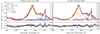 |
Fig. 5. Integrated quasar spectrum for J1120+0641 (black) showing the region around Hβ. The spectrum is integrated over a radius of |

Both models find a clear outflow component in the [O III] λλ4959,5007 and Hβ lines, fit by a Gaussian with velocity offset of  km/s (
 km/s) from the narrow-line component, and with
  km/s (
 km/s), for the DG (BPL) model. This outflow is spatially unresolved at the location of the quasar and is removed in the quasar subtraction process – from the low velocity offsets and velocity dispersions in the quasar-subtracted line maps (Figure 3) there is no signature of extended outflows or any indication that Regions 2 and 3 are outflowing gas. The quasar-driven outflow will be studied in depth alongside those of the full GA-NIFS quasar sample (Venturi et al., in prep.).
To calculate the BH mass, we used the commonly employed scaling relation
 (5)
(5)
which uses the continuum luminosity of the AGN at rest-frame λ = 5100 Å, L5100, the line width of the Hβ BLR component, FWHMHβ, and the constants a and b that are calibrated empirically from reverberation mapping studies. We consider the calibration a = (4.4 ± 0.2)×106, b = 0.64 ± 0.02 from Greene & Ho (2005), and alternatively a = (8.1 ± 0.4)×106, b = 0.50 ± 0.06 from Vestergaard & Peterson (2006). We could not measure L5100, as at the quasar redshift 5100 Å rest-frame falls into the gap between the two detectors. We instead used the value measured from the NIRCam grism spectra, of λL5100 = 1.76 × 1046 erg/s (Yue et al. 2024).
Alternatively, we considered the pure-Hβ scaling relation, which uses the Hβ BLR luminosity LHβ instead of the continuum luminosity:
 (6)
(6)
Again a and b are calibrated from low-z reverberation mapping studies; we considered both a = (3.6 ± 0.2)×106, b = 0.56 ± 0.02 from Greene & Ho (2005), and a = (4.7 ± 0.3) × 106, b = 0.63 ± 0.06 from Vestergaard & Peterson (2006). These scaling relations Equations (5) and (6) have an estimated scatter of 0.43 dex (Vestergaard & Peterson 2006).
The resulting Hβ BH mass estimates are given in Table 3, alongside the luminosities and FWHMs used in the calculations. We find that for the two BLR models (BPL and DG), the median 5100 Å-based measurement from Equation (5) is  . For the Greene & Ho (2005) Hβ-only based measurement from Equation (6), the median for the two models is
  . However, the Vestergaard & Peterson (2006) Hβ-only based measurements from Equation (6) are significantly larger, with median
  . Both of these empirical relations are based on low-z AGNs, and not high-z luminous quasars; these sources require extrapolation beyond the luminosity range of the observed low-z calibration sample. Thus, it seems likely that the disagreement of the Vestergaard & Peterson (2006) Hβ-only masses is due to this relation diverging from the Greene & Ho (2005) relation at AGN luminosities beyond the observed regime. Because three of the four relations produce BH masses that are in close agreement, we decide to disregard the Vestergaard & Peterson (2006) Hβ-only masses as outliers.
Estimated BH masses (MBH), Eddington ratios (λEdd), and the FWHMs and luminosities used in their calculation for the quasar J1120+0641.
We now compare how the different modelling assumptions alter the measured BH mass. Both the DG and BPL models provide very similar mass estimates, with the BPL model producing slightly larger estimates but being consistent within 1σ. The DG model measures a slightly larger Hβ luminosity than the BPL model, while the FWHM of the line is slightly lower for the DG model, although these estimates agree to within 1σ. The quoted uncertainties for each parameter are lower for the DG model, which has lower residuals around the Hβ line.
Taking the median of the BPL and DG masses over each of the three estimates per model, we obtain a best estimate BH mass of  . These uncertainties include only observational errors and do not include the scatter in the scaling relations Equations (5) and (6), estimated to be 0.43 dex from Vestergaard & Peterson (2006). Including the scaling relation uncertainties, we estimate
  .
.
Finally, we consider the effect of the host galaxy emission on the measured BH mass. We performed the same QubeSpec fitting process on the quasar model spectrum – the spectrum from the brightest spaxel in the cube, where the host contribution is negligible – with appropriate flux scaling correction. We also performed the QubeSpec fitting on an approximate host-subtracted spectrum – we integrated the quasar-subtracted cube over the same 0 35 aperture, and measured and removed its [O III] λλ4959,5007 line profile from the full integrated spectrum. We find that the BH masses measured from these spectra are 0.3 and 0.1 dex lower than our best estimate, respectively, although they are consistent within the 1σ measurement uncertainties; we conclude that the host galaxy emission does not significantly impact our BH mass measurement.
In Yue et al. (2024), the Hβ BH mass is measured from NIRCam grism spectra as MBH = (1.19 ± 0.08)×109 M⊙. Since we assume the same L5100, this lower estimate occurs due to their lower Hβ FWHM, which is  km/s, relative to our
  km/s from the DG model. While our BH mass and FWHM estimates are slightly larger, these are consistent within 2σ. Their NIRCam grism spectra has a spectral resolution of ∼1600 at 4 μm. In comparison, our IFU observations have a spectral resolution of ∼2700, which allowed us to conduct more detailed modelling. Our observations also include the [O III] λλ4959,5007 lines, while in the NIRCam grism these fall on the edge of the detector and cannot be well measured; these lines play a large role in constraining our MCMC fit, particularly with the iron template parameters. Yue et al. (2024) assumed a Hβ model composed of two Gaussians, which should be most consistent with our DG model. However, we also allowed a narrow and an outflow component to the Hβ line, but they did not, and this choice will make a small difference. Overall, with these differences in the measured spectra and modelling approaches, it is reasonable that we are measuring slightly different BH masses for the same Hβ line, although we reiterate that our masses are consistent within 2σ, and well below the systematic uncertainties (i.e. 0.43 dex).
With MIRI’s MRS, Bosman et al. (2024) obtained a spectrum of J1120+0641 that covers the Hα, Pa-α, Pa-β and Pa-γ emission lines. Using similar scaling relations to Equation (6), these lines were used to calculate BH masses that are: MBH, Hα = (1.55 ± 0.22)×109 M⊙,  , and
, and  . They also measured the BH mass using the combined Paschen-series lines and the rest-frame infrared continuum to be MBH, IR = (0.89 ± 0.14)×109 M⊙. These measurements have not been corrected for dust extinction, as they found by comparing the Hα and Paschen-series lines that minimal BLR extinction is present, of order E(B − V)≲0.1 (Bosman et al. 2024). The Hα BH mass is similar to our Hβ BH mass estimate, which we have also not corrected for dust attenuation; this is consistent with the quasar emission being minimally affected by dust. The Paschen-based BH masses are lower than our Hβ mass, although they are all consistent within 1σ when considering the additional uncertainty from the scaling relations. Overall, we conclude that the BH mass measurements measured by Bosman et al. (2024) with MIRI MRS are consistent with our Hβ BH mass measurement.
Finally, we compare the JWST BH mass estimates to the previous estimates from ground-based telescopes. From the Mg II emission line, the BH mass was measured to be  (Yang et al. 2021), which is consistent with our estimates. We note that the scaling relations for Mg II BH mass estimates have a scatter of ∼0.55 dex (Vestergaard & Osmer 2009), which is not included in the quoted uncertainties. From the C IV emission line, Farina et al. (2022) measured a BH mass of
  . Bosman et al. (2024) found that this C IV BH mass is not consistent with their Paschen-based BH masses, although it is consistent with their Hα mass. However, when considering that there is a scatter in the C IV scaling relations of ∼0.36–0.40 dex (Vestergaard & Peterson 2006; Shen & Liu 2012), this C IV BH mass is consistent with all of the above quoted BH masses.
Combining all of these independent observations and methods to estimate BH mass, we can be confident that the BH mass of J1120+0641 is generally in the range of ∼1–2 × 10⁹ M⊙, with the best estimate from this work being  .
.
3.3.2. Eddington ratio
To estimate the Eddington ratio λEdd = LBol/LEdd, we use the bolometric luminosity from Yue et al. (2024),  , as calculated from the rest-frame 5100 Å luminosity using the conversion LBol = 9.26 × λL5100 (Shen et al. 2011). We calculated the Eddington luminosity using
 (7)
(7)
where G is the gravitational constant, mp the proton mass, and σT the Thomson scattering cross-section. The Eddington ratios for each of our BH mass estimates are given in Table 3. For our 5100 Å Greene & Ho (2005) and Vestergaard & Peterson (2006), and Hβ-only Greene & Ho (2005) BH mass estimates, the Eddington ratio ranges from 0.6–0.8 for each of the models. For our best BH mass estimate of  , we estimate λEdd = 0.7 ± 0.1, or
  when including the 0.43 dex scatter in the BH scaling relations. Bosman et al. (2024) estimate λEdd = 0.9 ± 0.1 from Hα, using a slightly larger bolometric luminosity of
  from Farina et al. (2022), and Yue et al. (2024) estimate λEdd = 1.08 from Hβ, using the same LBol and a lower MBH; both are consistent with our measurement.
4. Host galaxy properties from NIRCam
4.1. Quasar subtraction and host modelling
From the [O III] λλ4959,5007 emission-line maps we discovered that the J1120+0641 system is comprised of both a quasar host galaxy and a merging companion galaxy. When Yue et al. (2024) performed their detailed quasar subtraction on NIRCam images, they modelled this host system with only one Sérsic profile. They were able to reveal the continuum emission surrounding J1120+0641, with clear detections in F356W and F200W, and a tentative detection in F115W. They found mF200W = 24.43 ± 0.10 mag and mF356W = 24.45 ± 0.20 mag, which resulted in a stellar mass estimate of  from SED fitting. The peak of this F200W and F356W continuum emission was offset by
  from the quasar–consistent with the location of the companion galaxy. These initial magnitude and mass estimates from Yue et al. (2024) included both of the host and companion components. In this work, we use the structure found from the IFU to improve the modelling of the system and the subsequent measured host stellar mass.
We used PSFMC to fit the NIRCam images of J1120+0641. We used a point source to describe the emission from the quasar, and used two exponential disks (Sérsic profiles with indices n = 1) to describe the extended emission from the quasar host galaxy (Region 1) and the close companion (Region 2). We note that J1120+0641 was visited four times in the EIGER program; following the method in Yue et al. (2024) we fit the images from the four visits individually, and take the mean and standard deviation of all of the MCMC samples from the four visits as the best-values and uncertainties of the model parameters. This approach allowed us to take into account the systematic uncertainties caused by inter-visit differences (e.g. the changes of PSF between the different pointings, which each have the quasar in a different detector location). If the magnitude error of the component is smaller than 0.3 mag, we consider the component to be detected in the image.
We first tried to fit the NIRCam images with all parameters allowed to vary (point source position and magnitude, Sérsic positions, magnitudes, major axis radii ra, minor axis radii rb, and position angles, with fixed Sérsic indices n = 1). However, the parameters related to Regions 1 and 2 (e.g. their sizes and ellipticities) did not converge to physical values. We thus fixed the spatial positions and morphological parameters of Regions 1 and 2 to the values measured in Section 3.1 from running psfMC on our [O III] λ5007 emission-line maps. In Figure 6 we show the F200W PSF-subtracted image overlaid with the [O III] λ5007 line map. The PSF-subtracted [O III] λ5007 and F200W maps largely overlap with each other, confirming that the extended continuum and line emission in J1120+0641 come from the same sources, the host galaxy and the close companion. The residual images also show faint positive flux in the north and south-west; the south-west structure corresponds to Region 3 seen in the IFU images, while the northern structure is not covered by the IFU. Additional residuals are most likely due to the host and companion not being ideally modelled by these Sérsic profiles.
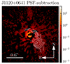 |
Fig. 6. Overlay plot of the F200W PSF-subtracted image (background image with colour bar) and the [O III] λ5007 map (white contour). The emission in the PSF-subtracted F200W image largely overlaps with the [O III] λ5007 line map, indicating that the continuum and line emission originate from the same objects, i.e. the quasar host and the close companion. The marked scale of 0 |

The full results of the image fitting are shown in Figure 7, with the extracted magnitudes given in Table 4. The PSF-subtracted images clearly show extended emission in all three bands, confirming the results from Yue et al. (2024). For the host galaxy (Region 1), the image fitting gives mF115W = 25.94 ± 0.20 mag, mF200W = 25.48 ± 0.37 mag and mF356W = 25.72 ± 0.47 mag. Given the above-mentioned detection criteria, Region 1 is only detected in F115W and has non-detections in F200W and F356W. For the companion (Region 2), we measure mF115W = 25.32 ± 0.12 mag, mF200W = 24.95 ± 0.11 mag and mF356W = 25.11 ± 0.18 mag, and so the companion is detected in all three bands. The quasar (i.e. the point source) has mF115W = 20.366 ± 0.003 mag, mF200W = 19.886 ± 0.002 mag and mF356W = 19.632 ± 0.003 mag. The host and the companion are ∼5 magnitudes fainter than the quasar. While their magnitudes are difficult to measure relative to the bright flux of the quasar, Yue et al. (2024) tested this methodology on mock quasar host observations and found that biases from this fitting process are low, smaller than the random error, providing confidence in these magnitude measurements.
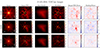 |
Fig. 7. Results from the NIRCam PSF subtraction for J1120+0641. From left to right, the original NIRCam images, the PSF-subtracted images, the model for the host and the companion, the image fitting residual (i.e. the subtraction of the full model from the original image), the PSF-subtracted images divided by the error images, and the residual images divided by the error images. The extended emission is modelled as two Sérsic profiles using the positions and morphologies as measured from the [O III] λ5007 maps (Section 3.1). The PSF-subtracted images clearly show the extended emission around the quasar. |
4.2. Spectral energy distribution fitting: Stellar population properties
We fit the SEDs of the quasar host and the companion using Prospector (Johnson et al. 2021) to constrain their stellar masses and other properties. Prospector is based on Flexible Stellar Population Synthesis (FSPS) and uses photoionisation predictions for nebular emission from Cloudy (e.g. Byler et al. 2017). The input observations are the host and companion Hβ, [O III] λ4959, and [O III] λ5007 line fluxes from Table 1, as well as their F115W, F200W, and F356W magnitudes from Table 4. We fit the SEDs of Region 1 (the host galaxy) and Region 2 (the companion) separately. Although we report non-detections for Region 1 in the F200W and the F356W bands, we still included these magnitudes and their errors when performing SED fitting for Region 1. This is because measurements with large uncertainties are preferred over upper limits in Prospector, as recommended in their documentation4.
Extracted NIRCam magnitudes for the quasar host and companion galaxy, and their stellar mass (M*), fraction of stars formed in the recent starburst (fstarburst), and metallicity (Z) measured from the subsequent SED fitting.
We used a Chabrier initial mass function (Chabrier 2003) and assumed a dust attenuation following the Calzetti et al. (2000) law. We considered two star-formation history (SFH) models when fitting the SED, namely, a delayed-τ model (SFR(t)∝te−t/τ), and a delayed-τ plus a starburst model. We also included an empirical template for emission-line flux produced by AGNs as included in Prospector, which is based on the observations of Richardson et al. (2014). The free parameters and their priors of this SED model include: (1) the stellar mass M* with a log-uniform prior at [108 M⊙, 1012 M⊙]; (2) the stellar metallicity log(Z/Z⊙) with a uniform prior at [ − 2, 0.2]; (3) the starting time of the star formation tage with a uniform prior at [0, t(z)], where t(z) is the age of the universe at the quasar’s redshift; (4) the exponential decay timescale τ with a uniform prior at [0.01 Myr, 20 Myr]; (5) the dust attenuation (quantified as the optical depth at 5500 Å, τ5500) with a uniform prior at [0, 2]; (6) the gas-phase metallicity log(Zg/Z⊙) with a uniform prior at [ − 2, 0.5]; (7) the ionisation parameter logU with a uniform prior at [ − 3, 1], and; (8) the flux scaling factor applied to the AGN emission-line template, with a uniform prior at [10−6, 10−2]. For the delayed-τ plus starburst SFH, there are two additional parameters: (9) the fraction of stellar mass produced by the starburst, fburst, with a uniform prior at [0, 1], and (10) the time of the starburst, tburst, with a uniform prior at [0, t(z)], which is also required to be later than tage.
The result of the SED fitting is shown in Figure 8. For both Region 1 and Region 2, the delayed-τ plus a starburst SFH gives the best description to the observed fluxes. We therefore used the delayed-τ plus a starburst SFH to infer the properties of the quasar host and its companion. The estimated physical parameters are listed in Table 4. The results of the SED fitting suggest that J1120+0641 might have a complex SFH that cannot be well-described by a single SFH component. For example, Figure 8 shows that the Hβ line is overestimated for both Regions 1 and 2 in both the delayed-τ and delayed-τ plus starburst models. The F200W fluxes for both regions are underestimated in both SFH models. This is likely due to an overestimation of the measured F200W flux in the quasar subtraction process, likely caused by slight inaccuracies in the PSF models, and the galaxies not being perfectly modelled by Sérsic profiles.
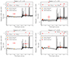 |
Fig. 8. Spectral energy distribution fitting for the host galaxy Region 1 (upper panels) and for the companion galaxy Region 2 (lower panels). The left and right columns correspond to a single delayed-τ SFH and a delayed-τ plus a starburst SFH, respectively. The red circles represent the NIRCam broad-band fluxes from image fitting, and the red triangles represent the observed Hβ and [O III] λλ4959,5007 line fluxes. The solid black line and the gray shaded region mark the Prospector modelled spectrum and its 1σ error, while the orange squares show the resulting model photometry. |
According to the SED models, the inferred stellar mass is  for Region 1 and
  for Region 2. The fraction of stellar mass formed by the starburst component is
  for Region 1 and is 0.99 ± 0.01 for Region 2. This suggests that the majority of the stars in the companion galaxy formed in a single past starburst, with little recent star formation. The SED models also provide constraints on the stellar metallicities, which are based on FSPS stellar population models. The metallicity of Region 1 is estimated to be log(Z/Z⊙)= − 0.50 ± 0.24, and the metallicity for Region 2 is
  . Our analysis demonstrates how we can constrain the SFH of quasar host galaxies by combining the broad-band fluxes from NIRCam imaging and emission-line fluxes from NIRSpec IFU.
As discussed in Section 3.1, both Regions 1 and 2 are likely photoionised by the central quasar based on the BPT diagnostic (Appendix B). Including the AGN emission-line template in our SED fitting allowed us to account for this excess non-star-formation photoionisation, in order to more accurately model the stellar population. If we exclude the AGN emission-line template and re-fit the SED models, assuming that the emission lines are entirely from star formation, we obtain slightly larger stellar masses of  for Region 1 and
  for Region 2. These estimates are consistent within our uncertainties (within 1σ for Region 1 and 2σ for Region 2), and the slight differences do not affect our conclusions. We can be confident that the host galaxy stellar mass is
  , with a broadly similar mass for the companion galaxy.
We end this section by comparing the results from this work and that from Yue et al. (2024). Yue et al. (2024) performed SED fitting using only the F200W and F356W magnitudes of the entire extended emission, which included both the quasar host and the companion. They assumed a delayed-τ SFH and inferred a stellar mass of  . Our host galaxy stellar mass estimate
  , and the combined total system mass
  are consistent with this original estimate, although our measurements have lower uncertainty due to the improved SED fitting from the addition of the NIRSpec IFU data. In this work, we show that a single delayed-τ model does not adequately describe the observations when we combine broad-band photometry and emission-line fluxes, and demonstrate that the SFH likely contains a starburst component. We are also able to constrain the metallicities of the quasar host galaxy and its companion. These comparisons emphasise the importance of emission-line measurements in understanding the co-evolution of high-redshift BHs and their host galaxies.
5. Discussion
5.1. Mass distribution in the system: Presence of an overmassive black hole
Using the PdBI, Venemans et al. (2012) detected the [C II] 158 μm emission-line and FIR-continuum luminosity of the host of J1120+0641, unresolved at the 2′′ resolution. They estimated a SFR between 160–440 M⊙/yr, a total dust mass of 0.67–5.7 × 10⁸ M⊙, and a dynamical mass of Mdyn < 3.6 × 10¹⁰sin(i)−2 M⊙. ALMA observations at higher  resolution improved on these measurements, although the emission is still only marginally resolved (Venemans et al. 2017). They estimated a SFR of 105–340 M⊙/yr, a dust mass of (0.8–4)×108 M⊙, and an upper limit of the dynamical mass of Mdyn < (4.3 ± 0.9)×1010 M⊙. From upper limits on the CO(2–1) and CO(7–6) lines, Venemans et al. (2017) estimate upper limits of the molecular gas mass of Mgas < 4 × 10¹⁰ M⊙. With higher resolution observations allowing for more accurate dynamical modelling, these mass estimates could likely be improved. However, it is reasonable to conservatively assume that the host total gas mass and dynamical mass are < 4 × 10¹⁰ M⊙, with a dust mass of Mdust < 109 M⊙. As we show in Section 5.2, the majority of the [C II] 158 μm and FIR continuum emission is from the host galaxy and not the companion, and so these measurements are unlikely to be significantly biased by the presence of the previously unknown companion. From our [O III] λλ4959,5007 emission-line maps, we estimate the quasar host to have a dynamical mass of
  , with the companion galaxy having
  . These are consistent with the dynamical mass and gas mass upper limits from ALMA.
From this work we estimate a stellar mass for the host galaxy of  . In the original Yue et al. (2024) work, they estimated a host stellar mass of
  . The primary differences in these estimations are due to an improved understanding of the system morphology (i.e. the presence of two separate galaxies instead of a single host), and an improved exponential decay plus starburst SFH model in the SED fitting. Overall, we can be confident that the host stellar mass is 109 ≲ M* ≲ 1010 M⊙. Thus, the stellar mass is greater than the dust mass of Mdust < 109 M⊙, and less than our best dynamical mass estimate of
  . If we assume that the gas mass can be estimated as Mgas = Mdyn − M*, we estimate
  , consistent with the upper limit of the gas mass from ALMA of Mgas < 4 × 10¹⁰ M⊙. This gives an estimate of the gas fraction of Mgas/Mdyn ≃ 0.76, while the dust fraction is Mdust/Mdyn < 0.08.
For J1120+0641, we can now be confident in the accuracy of the measured BH mass, with many independent estimates including three studies based on the broad hydrogen lines from the JWST observations of Yue et al. (2024), Bosman et al. (2024) and this work. As discussed in Section 3.3.1, we conclude that MBH ≃ 1–2 × 10⁹ M⊙. The estimates based on hydrogen lines are MBH = (0.87–1.9)×109 M⊙, including our best estimate  . The largest estimate is from C IV,
  (Farina et al. 2022).
With a stellar mass estimate of  , and hydrogen-based BH mass estimates of MBH = (0.87–1.9)×109 M⊙, the BH–stellar mass ratio for J1120+0641 is very high. For the minimum BH mass of
  from Paschen-β (Bosman et al. 2024),
  . The estimate of MBH = (1.55 ± 0.22)×109 M⊙ from Bosman et al. (2024), the largest hydrogen-based estimate excluding our measurement, corresponds to a ratio of
  . For our Hβ BH mass estimate of
  , we get a ratio of
  . Including the uncertainty in the BH mass scaling relations of 0.43 dex, which is not included in the Bosman et al. (2024) measurements, we obtain a ratio of
  .
.
We plot the BH–stellar mass relation in Figure 9, showing this best estimate for J1120+0641, alongside a range of data for comparison. The BH–stellar mass ratio is clearly much larger than expected from the local BH-stellar mass relations of Reines & Volonteri (2015) and Greene et al. (2020). Applying the Greene et al. (2020) scaling relation of MBH–M* to a stellar mass of  , the BH mass would be estimated as
  , with
  . Instead applying the Reines & Volonteri (2015)MBH–M* scaling relation, the BH mass would be estimated as
  , with
  . Clearly, our BH–stellar mass ratio of
  is much larger than these values, by order ∼3 dex, indicating that J1120+0641 has a very overmassive BH. There is significant scatter in the Reines & Volonteri (2015) and Greene et al. (2020) relations. Given the conservative uncertainty in our measured stellar and BH mass measurements, we find that J1120+0641 is 2.7σ above the Greene et al. (2020) relation, and 3.8σ above the Reines & Volonteri (2015) relation.
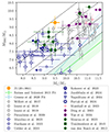 |
Fig. 9. Black hole–stellar mass relation showing the overmassive BH in J1120+0641 (gold). Purple points show z ≳ 6 quasars with stellar mass estimates from JWST (Ding et al. 2023; Yue et al. 2024). Pink points show dynamical mass measurements for z ≃ 6 quasars as measured with JWST (Marshall et al. 2023), while grey points show dynamical mass measurements as measured with ALMA (Willott et al. 2017; Izumi et al. 2018, 2019; Pensabene et al. 2020). Blue points show measurements for high-z AGNs discovered with JWST (Maiolino et al. 2024; Harikane et al. 2023; Übler et al. 2023; Kokorev et al. 2023; Juodžbalis et al. 2024; Furtak et al. 2024; Napolitano et al. 2024). Green points show samples of low-z sources with large MBH/M* ratios (Mezcua et al. 2023; Trakhtenbrot et al. 2015; van den Bosch et al. 2012). The grey dashed lines depict MBH/M* ratios of 0.1%, 1%, 10%, and 100%. The coloured curves show the local Reines & Volonteri (2015) and Greene et al. (2020) relations, with the shaded regions showing the ±1σ scatter in the relations, for comparison. |
Such an overmassive BH relative to its host galaxy is not unprecedented at high-z, as seen in Figure 9. Observations with JWST have been finding overmassive BHs at high-z. The quasar J0148+0600 at z = 5.98 has a BH–stellar mass ratio of ∼0.18 (Yue et al. 2024). Kokorev et al. (2023) discovered an AGN at z = 8.50 with a BH–stellar mass ratio of > 0.3. A z = 6.68 AGN was measured to have an extreme BH–stellar mass ratio of ∼0.4 (Juodžbalis et al. 2024). Maiolino et al. (2024) have found a range of low BH-mass (MBH < 107.5 M⊙) 4 < z < 11 sources with BH–stellar mass ratios of > 0.1. At lower redshifts, Trakhtenbrot et al. (2015) found an AGN in a typical star-forming galaxy at z = 3.3 with MBH/M* = 0.12. Mezcua et al. (2023) found that multiple broad-line AGNs in dwarf galaxies at z < 1 have MBH/M* > 0.1, with the largest two in the sample having MBH/M* = 0.32. van den Bosch et al. (2012) measured the local disc galaxy NGC 1277 to have MBH/M* = 0.14. Objects with such large MBH/M* are rare, and so while J1120+0641 may have the largest reported MBH/M* ratio to date of ≃0.63, this extreme ratio is not unprecedented.
Given the number of independent observations finding that MBH ≃ (1 − 2)×109 M⊙, the most likely way for us to have overestimated the BH–stellar mass ratio is if we have significantly underestimated the stellar mass. The bright quasar makes it significantly difficult to observe the host galaxy, with some non-detections in the NIRCam photometry. If the quasar was hiding a very bright, massive galaxy that was undetectable due to the difficulty in quasar subtraction, this could alleviate the very high BH–stellar mass ratio measured here. However, we would not expect a larger stellar mass than the dynamical mass we have measured,  . Thus the ratio
  , which further supports the BH being overmassive relative to its host. If we assume that our dynamical mass estimate is also biased due to the difficulty of the quasar subtraction, and instead use the ALMA dynamical mass estimate, at wavelengths where the quasar contribution is negligible, we have M* < Mdyn, ALMA < (4.3 ± 0.9)×1010 M⊙, or MBH/M* > 0.044. This would be a very conservative underestimate, as the dynamical mass has a significant contribution from the gas component of the galaxy. We could also consider the ‘galaxy stellar mass’ to be that of the host and companion galaxy combined:
  , and so
  . These various host mass estimates all support this being an overmassive BH. An alternative way for these ratios to be overestimated is if the BH masses are systematically overestimated. The BH mass scaling relations Equations (5) and (6) are calibrated using low-z AGNs, and so these may not accurately describe high-z sources; if these scaling relations overestimate BH mass at high-z, this could also reduce the BH–stellar mass ratio for this system. A recent dynamical BH mass measurement at z = 2.3 found that the Hα-based scaling relation overestimated the BH mass by 0.43 dex (Abuter et al. 2024), however, this is consistent with the known scatter in the relation that our uncertainties account for.
5.2. Comparison with emission seen with ALMA
We obtained the archival data from the Venemans et al. (2017) ALMA observations (ALMA project code 2012.1.00882.S) to compare their [C II] 158 μm properties to our measurements. We made a [C II] 158 μm integrated intensity (moment 0) map with a natural weighting and resolution of 0 3 as well as a FIR continuum intensity map of the 158 μm rest-frame dust emission. These are overlaid onto our [O III] λ5007 map in Figure 2. This [C II] 158 μm emission matches the spatial location of the [O III] λ5007 emission from the host galaxy well, although shows a more symmetrical, round structure than the elongated [O III] λ5007 system. No [C II] 158 μm emission is seen from the companion galaxy at this sensitivity. The FIR continuum emission follows a very similar shape, with no emission from the companion galaxy detected.
Based on the [C II] 158 μm line detection of the quasar host, with flux F[CII] = 1.11 ± 0.1 Jy km/s and L[CII] = (1.5 ± 0.1)×109 L⊙, Venemans et al. (2017) derive a SFR of 80–500 M⊙/yr. This uses the high-redshift L[CII]–SFR scaling relation of De Looze et al. (2014). Given the non-detection of the companion in the ALMA data, the companion galaxy must have a lower SFR than the quasar host. Following the Venemans et al. (2017) methodology, and using their quoted RMS noise level of 0.042 Jy km/s, for the companion galaxy we estimate L[CII] < 1.75 × 10⁸ L⊙ at the 3σ level, which corresponds to SFR < 40 M⊙/yr. If the companion galaxy is on the star forming main sequence, with stellar mass  it would have a SFR of
  /yr (Popesso et al. 2023), below the ALMA detection limit. Thus the ALMA non-detection only confirms that, unlike the quasar host, the companion galaxy is not an extreme star forming galaxy above the main sequence.
We also estimated the SFRs from the integrated flux of the narrow Hβ line (Table 1) using
 (8)
(8)
(Kennicutt & Evans 2012). This conversion assumes no dust extinction, a solar abundance, and a Kroupa IMF, and uses the theoretical conversion from Hα to Hβ flux of FHα/FHβ = 2.86, which assumes a temperature T = 104 K and an electron density  for Case B recombination (Osterbrock 1989; Domínguez et al. 2013). If we assume that all of the quasar-subtracted Hβ narrow-line flux measured in Table 1 is from star formation, with no contribution from quasar photoionisation, we obtain SFRs of < 20 M⊙/yr for the host galaxy, and 3.6 M⊙/yr for the companion galaxy. For the quasar host, the Hβ SFR is much lower than the [C II] 158 μm-estimated value of 80–500 M⊙/yr. Some of this discrepancy is likely explained by Hβ and [C II] 158 μm tracing star formation on different time scales. In addition, Hβ will be affected by dust-attenuation, which we have not corrected for–Hβ would give a lower estimate of the SFR as the [C II] 158 μm measure includes dust-obscured star formation. With a very low Hβ SFR of 3.6 M⊙/yr, the companion galaxy is either significantly below the star forming main sequence or has substantial dust-obscured star formation. The ALMA limit of < 40 M⊙/yr does not differentiate between these two possibilities.
This major merger may be triggering both a starburst and AGN activity in the quasar host galaxy. Theory predicts that galaxy mergers can induce AGN activity, due to torques funnelling gas into the centre of the galaxy (Hernquist & Mihos 1995), as well as star formation episodes (e.g. Doyon et al. 1994; Mihos & Hernquist 1996). In gas-rich mergers, an AGN phase followed by a starburst is a common evolutionary sequence (Hopkins et al. 2006; Melnick et al. 2015).
5.3. Location of the black hole relative to the gas and stellar components
When comparing the spatial location of the quasar to the full structure of this system from PSF-subtracted emission maps in Figures 2 and 3, the quasar is offset to the north-east of the centre of the emission. However, the detail of the IFU observations reveals that this is because there is a separate companion galaxy in the south-west, and that the quasar is indeed at the centre of its host galaxy, as typically expected. From the NIRCam imaging the quasar similarly appeared offset from the peak of the continuum emission; without the information gained from the IFU, this could be incorrectly interpreted as the quasar being offset from the centre of its host galaxy.
GA-NIFS observations of DELS J0411−0907 and VDES J0020−3653 at z = 6.8 also revealed that these quasars are undergoing mergers (Marshall et al. 2023). For DELS J0411−0907 there are emission-line structures on both sides of the quasar host, meaning that the quasar still appears in the centre of the structure by chance. The companion galaxies around VDES J0020−3653 appear only to its south and west, and so without the detail of the IFU observations this quasar would appear to be offset from the centre of the system. Crucially, the detailed spectral decomposition provided by the IFU reveals that all of the GA-NIFS quasars analysed so far are located approximately at the centre of their host galaxies.
In general, a physical offset of the BH from the galaxy centre is possible. Observations have found a range of AGNs that are offset from their host’s centres on scales of up to tens of kiloparsecs (e.g. Clements et al. 2009; Koss et al. 2014; Liu et al. 2024). These offset BHs may be in the process of merging into the central nucleus (e.g. Übler et al. 2024) or may be recoiling, due to the emission of gravitational waves or a slingshot effect from triple BH systems (e.g. Komossa et al. 2008; Civano et al. 2010; Chiaberge et al. 2025). However, if a high-z quasar has an apparent spatial offset from the peak of observed galaxy emission, we caution this from being attributed to a potential offset BH from the centre of its host; the presence of close companions and irregular galaxy structures due to interactions may be a more likely option given the quasars observed with the IFU so far.
6. Conclusions
In this paper we have presented the GA-NIFS NIRSpec IFU observations of the z = 7.08 quasar J1120+0641. This gives spatially resolved imaging spectroscopy covering the 3′′ × 3′′ FOV around the quasar from 2.9–5.3 μm, which covers the key emission lines Hβ and [O III] λλ4959,5007 for this system. From the integrated quasar spectrum, we measured the BH mass and Eddington ratio from the broad Hβ line to be  and λEdd = 0.7 ± 0.1. These values are
  and
and  when considering the scatter in the BH scaling relations, which are consistent with previous JWST-based estimates.
We studied the extended host galaxy emission in [O III] λλ4959,5007 and Hβ by removing the quasar emission from the data cube. We discovered a companion galaxy interacting with the quasar host, ∼0 5 south-west of the quasar, with a velocity offset of 21 ± 49 km/s. The small projected distance to the quasar host and the low relative velocity imply that both galaxies form a merging system. Assuming a rotating disc geometry for both galaxies, we estimate dynamical masses of
  for the quasar host and
  for the companion galaxy. These estimates indicate that both galaxies have similar masses, and therefore they will experience a ‘major’ merger event.
By combining the IFU data with NIRCam imaging from the EIGER programme (Yue et al. 2024), we re-estimated the stellar mass of the host galaxy. We fixed the modelled continuum morphology to match the separate host and companion galaxy morphologies measured from our [O III] λ5007 map, and we used the measured Hβ and [O III] λλ4959,5007 line fluxes in the SED fitting. We estimate the host stellar mass to be  , with
  for the companion galaxy, which is consistent with this being a major merger system. The SED fitting favours a model where both galaxies have undergone a recent starburst. The addition of the IFU data provides a more accurate host stellar mass measurement than the original Yue et al. (2024) estimate of
  .
.
With a stellar mass estimate of  and our Hβ BH mass estimate of
  , we measure an extreme BH–stellar mass ratio of
  . J1120+0641 has an overmassive BH relative to its host galaxy. Notably, it is the largest BH–stellar mass ratio measured to date. This ratio is ∼3 dex larger than expected from the local Reines & Volonteri (2015) and Greene et al. (2020) scaling relations, but such an overmassive BH is not unprecedented at these redshifts (Yue et al. 2024; Kokorev et al. 2023; Maiolino et al. 2024; Juodžbalis et al. 2024).
Overall, this work highlights the power of using both NIRSpec IFU and NIRCam imaging together to understand high-z quasars, their host galaxies, and local environments. The IFU allows for measurements of BH mass as well as key galaxy emission lines. While the spatial sampling is coarser than that of NIRCam images, the relative ease of IFU quasar subtraction makes it easier to see the structure of the host galaxy and any companion galaxies, and it also provides kinematics. However, the high spectral resolution IFU mode is not sensitive to the faint continuum emission of most high-redshift systems. In such cases, NIRCam imaging can detect the continuum emission, which can be used to determine the host stellar mass. With the NIRSpec IFU providing the spatial structure and emission-line fluxes to improve the SED fitting, combining these observations gives more accurate stellar mass estimates. Used in this way, the two JWST instruments can work in synergy to provide a deeper understanding of high-z quasar hosts.
Acknowledgments
This work is based on observations made with the NASA/ESA/CSA James Webb Space Telescope. The data were obtained from the Mikulski Archive for Space Telescopes at the Space Telescope Science Institute, which is operated by the Association of Universities for Research in Astronomy, Inc., under NASA contract NAS 5-03127 for JWST. These observations are associated with program #1263, as part of the Galaxy Assembly with NIRSpec Integral Field Spectroscopy GTO program, and program #1243, as part of the Emission-line galaxies and Intergalactic Gas in the Epoch of Reionization GTO program. We thank Ignas Juodžbalis for helping with the compilation of BH–stellar mass measurements from the literature. We thank the referee for their helpful feedback. MAM acknowledges support by the Laboratory Directed Research and Development program of Los Alamos National Laboratory under project number 20240752PRD1. The project leading to this publication has received support from ORP, that is funded by the European Union’s Horizon 2020 research and innovation programme under grant agreement No 101004719 [ORP]. MP, SA and BRdP acknowledge grant PID2021-127718NB-I00 funded by the Spanish Ministry of Science and Innovation/State Agency of Research (MICIN/AEI/ 10.13039/501100011033). JS, RM and FDE acknowledge support by the Science and Technology Facilities Council (STFC), from the ERC Advanced Grant 695671 “QUENCH”. JS and FDE acknowledge the UKRI Frontier Research grant RISEandFALL. RM acknowledges funding from a research professorship from the Royal Society. HÜ acknowledges funding by the European Union (ERC APEX, 101164796). Views and opinions expressed are however those of the authors only and do not necessarily reflect those of the European Union or the European Research Council Executive Agency. Neither the European Union nor the granting authority can be held responsible for them. SC and GV acknowledge support from the European Union (ERC, WINGS,101040227). AJB and GCJ acknowledge funding from the “FirstGalaxies” Advanced Grant from the European Research Council (ERC) under the European Union’s Horizon 2020 research and innovation programme (Grant agreement No. 789056). DK acknowledges funding from JSPS KAKENHI Grant Number JP21K13956. This research has made use of the Astrophysics Data System, funded by NASA under Cooperative Agreement 80NSSC21M00561, QFitsView (Ott 2012), and SAOImageDS9, developed by Smithsonian Astrophysical Observatory. This paper made use of Python packages and software AstroPy (Astropy Collaboration 2013), jwst (Bushouse et al. 2022), Matplotlib (Hunter 2007), NumPy (van der Walt et al. 2011), Pandas (Pandas Development Team 2020), Photutils (Bradley et al. 2018), Prospector (Johnson et al. 2021), psfMC (Mechtley 2019), Regions (Bradley et al. 2022), SciPy (Virtanen et al. 2020), Seaborn (Waskom 2021), Spectral Cube (Ginsburg et al. 2019), QDeblend3D (Husemann et al. 2013, 2014), QubeSpec (https://github.com/honzascholtz/Qubespec), and WebbPSF (Perrin et al. 2015).
References
- Abazajian, K. N., Adelman-McCarthy, J. K., Agüeros, M. A., et al. 2009, ApJS, 182, 543 [Google Scholar]
- Abuter, R., Allouche, F., Amorim, A., et al. 2024, Nature, 627, 281 [NASA ADS] [CrossRef] [Google Scholar]
- Anderson, J., Fall, S. M., & Astrometry Working Group 2021, The JWST Calibration Field: Absolute Astrometry and Proper Motions with GAIA and a Second HST Epoch, Technical Report JWST-STScI-007716 [Google Scholar]
- Astropy Collaboration (Robitaille, T. P., et al.) 2013, A&A, 558, A33 [NASA ADS] [CrossRef] [EDP Sciences] [Google Scholar]
- Baldwin, J. A., Phillips, M. M., & Terlevich, R. 1981, PASP, 93, 5 [Google Scholar]
- Bañados, E., Decarli, R., Walter, F., et al. 2015, ApJ, 805, L8 [CrossRef] [Google Scholar]
- Bañados, E., Venemans, B. P., Decarli, R., et al. 2016, ApJS, 227, 11 [Google Scholar]
- Bañados, E., Venemans, B. P., Mazzucchelli, C., et al. 2018, Nature, 553, 473 [Google Scholar]
- Bañados, E., Schindler, J.-T., Venemans, B. P., et al. 2022, ApJS, 265, 29 [Google Scholar]
- Bennert, V. N., Auger, M. W., Treu, T., Woo, J.-H., & Malkan, M. A. 2011, ApJ, 726, 59 [NASA ADS] [CrossRef] [Google Scholar]
- Bertoldi, F., Cox, P., Neri, R., et al. 2003, A&A, 409, L47 [NASA ADS] [CrossRef] [EDP Sciences] [Google Scholar]
- Böker, T., Arribas, S., Lützgendorf, N., et al. 2022, A&A, 661, A82 [NASA ADS] [CrossRef] [EDP Sciences] [Google Scholar]
- Böker, T., Beck, T. L., Birkmann, S. M., et al. 2023, PASP, 135, 038001 [CrossRef] [Google Scholar]
- Boroson, T. A., & Green, R. F. 1992, ApJS, 80, 109 [Google Scholar]
- Bosman, S. E. I., Álvarez-Márquez, J., Colina, L., et al. 2024, Nat. Astron., 8, 1054 [NASA ADS] [CrossRef] [Google Scholar]
- Bradley, L., Sipocz, B., Robitaille, T., et al. 2018, https://doi.org/10.5281/zenodo.1340699 [Google Scholar]
- Bradley, L., Deil, C., Ginsburg, A., et al. 2022, https://doi.org/10.5281/zenodo.7259631 [Google Scholar]
- Bushouse, H., Eisenhamer, J., Dencheva, N., et al. 2022, https://doi.org/10.5281/zenodo.7229890 [Google Scholar]
- Byler, N., Dalcanton, J. J., Conroy, C., & Johnson, B. D. 2017, ApJ, 840, 44 [Google Scholar]
- Calzetti, D., Armus, L., Bohlin, R. C., et al. 2000, ApJ, 533, 682 [NASA ADS] [CrossRef] [Google Scholar]
- Cameron, A. J., Saxena, A., Bunker, A. J., et al. 2023, A&A, 677, A115 [NASA ADS] [CrossRef] [EDP Sciences] [Google Scholar]
- Cappellari, M., Bacon, R., Bureau, M., et al. 2006, MNRAS, 366, 1126 [Google Scholar]
- Chabrier, G. 2003, PASP, 115, 763 [Google Scholar]
- Chiaberge, M., Morishita, T., Boschini, M., et al. 2025, ArXiv e-prints [arXiv:2501.18730] [Google Scholar]
- Civano, F., Elvis, M., Lanzuisi, G., et al. 2010, ApJ, 717, 209 [NASA ADS] [CrossRef] [Google Scholar]
- Clements, D. L., Petitpas, G., Farrah, D., et al. 2009, ApJ, 698, L188 [NASA ADS] [CrossRef] [Google Scholar]
- Coatman, L., Hewett, P. C., Banerji, M., & Richards, G. T. 2016, MNRAS, 461, 647 [NASA ADS] [CrossRef] [Google Scholar]
- Conselice, C. J., Yang, C., & Bluck, A. F. L. 2009, MNRAS, 394, 1956 [NASA ADS] [CrossRef] [Google Scholar]
- Cresci, G., Mainieri, V., Brusa, M., et al. 2015, ApJ, 799, 82 [Google Scholar]
- Croton, D. J. 2006, MNRAS, 369, 1808 [NASA ADS] [CrossRef] [Google Scholar]
- da Silva, R. L., Prochaska, J. X., Rosario, D., Tumlinson, J., & Tripp, T. M. 2011, ApJ, 735, 54 [Google Scholar]
- De Looze, I., Cormier, D., Lebouteiller, V., et al. 2014, A&A, 568, A62 [NASA ADS] [CrossRef] [EDP Sciences] [Google Scholar]
- Decarli, R., Walter, F., Yang, Y., et al. 2012, ApJ, 756, 150 [NASA ADS] [CrossRef] [Google Scholar]
- Decarli, R., Walter, F., Venemans, B. P., et al. 2017, Nature, 545, 457 [Google Scholar]
- Decarli, R., Walter, F., Venemans, B. P., et al. 2018, ApJ, 854, 97 [Google Scholar]
- Decarli, R., Dotti, M., Bañados, E., et al. 2019, ApJ, 880, 157 [Google Scholar]
- Decarli, R., Loiacono, F., Farina, E. P., et al. 2024, A&A, 689, A219 [NASA ADS] [CrossRef] [EDP Sciences] [Google Scholar]
- D’Eugenio, F., Pérez-González, P. G., Maiolino, R., et al. 2024, Nat. Astron., 8, 1443 [CrossRef] [Google Scholar]
- Di Matteo, T., Springel, V., & Hernquist, L. 2005, Nature, 433, 604 [NASA ADS] [CrossRef] [Google Scholar]
- Ding, X., Onoue, M., Silverman, J. D., et al. 2023, Nature, 621, 51 [NASA ADS] [CrossRef] [Google Scholar]
- Domínguez, A., Siana, B., Henry, A. L., et al. 2013, ApJ, 763, 145 [CrossRef] [Google Scholar]
- Doyon, R., Joseph, R. D., & Wright, G. S. 1994, ApJ, 421, 101 [Google Scholar]
- Dunlop, J. S., McLure, R. J., Kukula, M. J., et al. 2003, MNRAS, 340, 1095 [NASA ADS] [CrossRef] [Google Scholar]
- Eilers, A.-C., Simcoe, R. A., Yue, M., et al. 2023, ApJ, 950, 68 [CrossRef] [Google Scholar]
- Fan, X., White, R. L., Davis, M., et al. 2000, AJ, 120, 1167 [NASA ADS] [CrossRef] [Google Scholar]
- Fan, X., Narayanan, V. K., Lupton, R. H., et al. 2001, AJ, 122, 2833 [Google Scholar]
- Fan, X., Strauss, M. A., Schneider, D. P., et al. 2003, AJ, 125, 1649 [Google Scholar]
- Farina, E. P., Schindler, J.-T., Walter, F., et al. 2022, ApJ, 941, 106 [NASA ADS] [CrossRef] [Google Scholar]
- Floyd, D. J. E., Dunlop, J. S., Kukula, M. J., et al. 2013, MNRAS, 429, 2 [NASA ADS] [CrossRef] [Google Scholar]
- Furtak, L. J., Labbé, I., Zitrin, A., et al. 2024, Nature, 628, 57 [NASA ADS] [CrossRef] [Google Scholar]
- Gaia Collaboration (Brown, A. G. A., et al.) 2018, A&A, 616, A1 [NASA ADS] [CrossRef] [EDP Sciences] [Google Scholar]
- Gardner, J. P., Mather, J. C., Clampin, M., et al. 2006, SSRv, 123, 485 [NASA ADS] [Google Scholar]
- Gardner, J. P., Mather, J. C., Abbott, R., et al. 2023, PASP, 135, 068001 [NASA ADS] [CrossRef] [Google Scholar]
- Ginsburg, A., Koch, E., Robitaille, T., et al. 2019, https://doi.org/10.5281/zenodo.3558614 [Google Scholar]
- Greene, J. E., & Ho, L. C. 2005, ApJ, 630, 122 [NASA ADS] [CrossRef] [Google Scholar]
- Greene, J. E., Strader, J., & Ho, L. C. 2020, ARA&A, 58, 257 [Google Scholar]
- Harikane, Y., Zhang, Y., Nakajima, K., et al. 2023, ApJ, 959, 39 [NASA ADS] [CrossRef] [Google Scholar]
- Häring, N., & Rix, H.-W. 2004, ApJ, 604, L89 [Google Scholar]
- Hernquist, L., & Mihos, J. C. 1995, ApJ, 448, 41 [NASA ADS] [CrossRef] [Google Scholar]
- Hinshaw, G., Larson, D., Komatsu, E., et al. 2013, ApJS, 208, 19 [Google Scholar]
- Hopkins, P. F., Hernquist, L., Cox, T. J., et al. 2006, ApJS, 163, 1 [Google Scholar]
- Hunter, J. D. 2007, CiSE, 9, 90 [Google Scholar]
- Husemann, B., Wisotzki, L., Sánchez, S. F., & Jahnke, K. 2013, A&A, 549, A43 [NASA ADS] [CrossRef] [EDP Sciences] [Google Scholar]
- Husemann, B., Jahnke, K., Sánchez, S. F., et al. 2014, MNRAS, 443, 755 [NASA ADS] [CrossRef] [Google Scholar]
- Hutchings, J. B. 2003, AJ, 125, 1053 [NASA ADS] [CrossRef] [Google Scholar]
- Izumi, T., Onoue, M., Shirakata, H., et al. 2018, PASJ, 70, 36 [NASA ADS] [Google Scholar]
- Izumi, T., Onoue, M., Matsuoka, Y., et al. 2019, PASJ, 71, 111 [CrossRef] [Google Scholar]
- Jakobsen, P., Ferruit, P., de Oliveira, C. A., et al. 2022, A&A, 661, A80 [NASA ADS] [CrossRef] [EDP Sciences] [Google Scholar]
- Ji, X., Li, C., Yan, R., et al. 2021, MNRAS, 508, 3943 [Google Scholar]
- Ji, X., Übler, H., Maiolino, R., et al. 2024, MNRAS, 535, 881 [NASA ADS] [CrossRef] [Google Scholar]
- Johnson, B. D., Leja, J., Conroy, C., & Speagle, J. S. 2021, ApJS, 254, 22 [NASA ADS] [CrossRef] [Google Scholar]
- Jones, G. C., Übler, H., Perna, M., et al. 2024, A&A, 682, A122 [NASA ADS] [CrossRef] [EDP Sciences] [Google Scholar]
- Juodžbalis, I., Maiolino, R., Baker, W. M., et al. 2024, Nature, 636, 594 [CrossRef] [Google Scholar]
- Kashikawa, N., Ishizaki, Y., Willott, C. J., et al. 2015, ApJ, 798, 28 [Google Scholar]
- Kashino, D., Lilly, S. J., Matthee, J., et al. 2023, ApJ, 950, 66 [CrossRef] [Google Scholar]
- Kaspi, S., Brandt, W. N., Maoz, D., et al. 2021, ApJ, 915, 129 [NASA ADS] [CrossRef] [Google Scholar]
- Kauffmann, G., Heckman, T. M., Tremonti, C., et al. 2003, MNRAS, 346, 1055 [Google Scholar]
- Keel, W. C., Bennert, V. N., Pancoast, A., et al. 2019, MNRAS, 483, 4847 [NASA ADS] [Google Scholar]
- Kennicutt, R. C., & Evans, N. J. 2012, ARA&A, 50, 531 [NASA ADS] [CrossRef] [Google Scholar]
- Kewley, L. J., Dopita, M. A., Sutherland, R. S., Heisler, C. A., & Trevena, J. 2001, ApJ, 556, 121 [Google Scholar]
- Kokorev, V., Fujimoto, S., Labbe, I., et al. 2023, ApJ, 957, L7 [NASA ADS] [CrossRef] [Google Scholar]
- Komossa, S., Zhou, H., & Lu, H. 2008, ApJ, 678, L81 [CrossRef] [Google Scholar]
- Kormendy, J., & Ho, L. C. 2013, ARA&A, 51, 511 [Google Scholar]
- Koss, M., Blecha, L., Mushotzky, R., et al. 2014, MNRAS, 445, 515 [NASA ADS] [CrossRef] [Google Scholar]
- Kovacevic, J., Popovic, L. C., & Dimitrijevic, M. S. 2010, ApJS, 189, 15 [CrossRef] [Google Scholar]
- Kuraszkiewicz, J. K., Green, P. J., Forster, K., et al. 2002, ApJS, 143, 257 [NASA ADS] [CrossRef] [Google Scholar]
- Lamperti, I., Arribas, S., Perna, M., et al. 2024, A&A, 691, A153 [NASA ADS] [CrossRef] [EDP Sciences] [Google Scholar]
- Larson, R. L., Finkelstein, S. L., Kocevski, D. D., et al. 2023, ApJ, 953, L29 [NASA ADS] [CrossRef] [Google Scholar]
- Law, D. D., Morrison, J. E., Argyriou, I., et al. 2023, AJ, 166, 45 [NASA ADS] [CrossRef] [Google Scholar]
- Lawrence, A., Warren, S. J., Almaini, O., et al. 2007, MNRAS, 379, 1599 [Google Scholar]
- Li, J., Silverman, J. D., Shen, Y., et al. 2025, ApJ, 981, 19 [Google Scholar]
- Liu, F.-Y., Dai, Y. S., Omont, A., et al. 2024, ApJ, 964, 136 [Google Scholar]
- Loiacono, F., Decarli, R., Mignoli, M., et al. 2024, A&A, 685, A121 [NASA ADS] [CrossRef] [EDP Sciences] [Google Scholar]
- Magorrian, J., Tremaine, S., Richstone, D., et al. 1998, AJ, 115, 2285 [Google Scholar]
- Maiolino, R., Scholtz, J., Curtis-Lake, E., et al. 2024, A&A, 691, A145 [NASA ADS] [CrossRef] [EDP Sciences] [Google Scholar]
- Marconi, A., & Hunt, L. K. 2003, ApJ, 589, L21 [Google Scholar]
- Marshall, M. A., Mechtley, M., Windhorst, R. A., et al. 2020, ApJ, 900, 21 [NASA ADS] [CrossRef] [Google Scholar]
- Marshall, M. A., Perna, M., Willott, C. J., et al. 2023, A&A, 678, A191 [NASA ADS] [CrossRef] [EDP Sciences] [Google Scholar]
- Matsuoka, Y., Onoue, M., Kashikawa, N., et al. 2018, PASJ, 70, S35 [Google Scholar]
- Matthee, J., Mackenzie, R., Simcoe, R. A., et al. 2023, ApJ, 950, 67 [NASA ADS] [CrossRef] [Google Scholar]
- Matthee, J., Naidu, R. P., Brammer, G., et al. 2024, ApJ, 963, 129 [NASA ADS] [CrossRef] [Google Scholar]
- Mazzucchelli, C., Bañados, E., Venemans, B. P., et al. 2017, ApJ, 849, 91 [Google Scholar]
- Mazzucchelli, C., Decarli, R., Belladitta, S., et al. 2025, A&A, 694, A171 [NASA ADS] [CrossRef] [EDP Sciences] [Google Scholar]
- McElwain, M. W., Feinberg, L. D., Perrin, M. D., et al. 2023, PASP, 135, 058001 [NASA ADS] [CrossRef] [Google Scholar]
- McGreer, I. D., Fan, X., Strauss, M. A., et al. 2014, AJ, 148, 73 [NASA ADS] [CrossRef] [Google Scholar]
- McLeod, K. K., & Rieke, G. H. 1994, ApJ, 420, 58 [CrossRef] [Google Scholar]
- Mechtley, M. 2019, psfMC https://github.com/mmechtley/psfMC [Google Scholar]
- Mechtley, M., Windhorst, R. A., Ryan, R. E., et al. 2012, ApJ, 756, L38 [NASA ADS] [CrossRef] [Google Scholar]
- Mechtley, M., Jahnke, K., Windhorst, R. A., et al. 2016, ApJ, 830, 156 [NASA ADS] [CrossRef] [Google Scholar]
- Melnick, J., Telles, E., De Propris, R., & Chu, Z.-H. 2015, A&A, 582, A37 [NASA ADS] [CrossRef] [EDP Sciences] [Google Scholar]
- Merluzzi, P., Busarello, G., Dopita, M. A., et al. 2018, ApJ, 852, 113 [Google Scholar]
- Mezcua, M., Siudek, M., Suh, H., et al. 2023, ApJ, 943, L5 [NASA ADS] [CrossRef] [Google Scholar]
- Mihos, J. C., & Hernquist, L. 1996, ApJ, 464, 641 [Google Scholar]
- Moiseev, A. V., Smirnova, A. A., & Movsessian, T. A. 2023, Universe, 9, 493 [Google Scholar]
- Moran, E. C., Halpern, J. P., Bothun, G. D., & Becker, R. H. 1992, AJ, 104, 990 [Google Scholar]
- Mortlock, D. J., Warren, S. J., Venemans, B. P., et al. 2011, Nature, 474, 616 [Google Scholar]
- Moseley, S. H., Arendt, R. G., Fixsen, D. J., et al. 2010, Proc. SPIE, 7742, 77421B [NASA ADS] [CrossRef] [Google Scholar]
- Nagao, T., Marconi, A., & Maiolino, R. 2006, A&A, 447, 157 [NASA ADS] [CrossRef] [EDP Sciences] [Google Scholar]
- Napolitano, L., Castellano, M., Pentericci, L., et al. 2024, ApJ, accepted [arXiv:2410.18763] [Google Scholar]
- Neeleman, M., Novak, M., Venemans, B. P., et al. 2021, ApJ, 911, 141 [NASA ADS] [CrossRef] [Google Scholar]
- Osterbrock, D. E. 1989, Astrophysics of Gaseous Nebulae and Active Galactic Nuclei (University Science Books) [Google Scholar]
- Ott, T. 2012, Astrophysics Source Code Library [record ascl:1210.019] [Google Scholar]
- Pacucci, F., Nguyen, B., Carniani, S., Maiolino, R., & Fan, X. 2023, ApJ, 957, L3 [CrossRef] [Google Scholar]
- Pan, H.-A., Lin, L., Hsieh, B.-C., et al. 2020, ApJ, 903, 16 [Google Scholar]
- Pandas Development Team. 2020, https://doi.org/10.5281/zenodo.3509134 [Google Scholar]
- Park, D., Barth, A. J., Ho, L. C., & Laor, A. 2022, ApJS, 258, 38 [NASA ADS] [CrossRef] [Google Scholar]
- Patton, D. R., Carlberg, R. G., Marzke, R. O., et al. 2000, ApJ, 536, 153 [NASA ADS] [CrossRef] [Google Scholar]
- Pensabene, A., Carniani, S., Perna, M., et al. 2020, A&A, 637, A84 [NASA ADS] [CrossRef] [EDP Sciences] [Google Scholar]
- Perna, M., Arribas, S., Marshall, M., et al. 2023, A&A, 679, A89 [NASA ADS] [CrossRef] [EDP Sciences] [Google Scholar]
- Perna, M., Arribas, S., Lamperti, I., et al. 2025, A&A, 696, A59 [NASA ADS] [CrossRef] [EDP Sciences] [Google Scholar]
- Perrin, M. D., Long, J., Sivaramakrishnan, A., et al. 2015, WebbPSF: James Webb Space Telescope PSF Simulation Tool [record ascl:1504.007] [Google Scholar]
- Peterson, B. M. 2009, Proc. Int. Astron. Union, 5, 151 [CrossRef] [Google Scholar]
- Popesso, P., Concas, A., Cresci, G., et al. 2023, MNRAS, 519, 1526 [Google Scholar]
- Protušová, K., Bosman, S. E. I., Wang, F., et al. 2024, A&A, 700, A218 [Google Scholar]
- Rauscher, B. J., Arendt, R. G., Fixsen, D. J., et al. 2017, PASP, 129, 105003 [NASA ADS] [CrossRef] [Google Scholar]
- Reines, A. E., & Volonteri, M. 2015, ApJ, 813, 82 [NASA ADS] [CrossRef] [Google Scholar]
- Richardson, C. T., Allen, J. T., Baldwin, J. A., Hewett, P. C., & Ferland, G. J. 2014, MNRAS, 437, 2376 [NASA ADS] [CrossRef] [Google Scholar]
- Rieke, G. H., Wright, G. S., Böker, T., et al. 2015, PASP, 127, 584 [NASA ADS] [CrossRef] [Google Scholar]
- Rieke, M. J., Kelly, D. M., Misselt, K., et al. 2023, PASP, 135, 028001 [CrossRef] [Google Scholar]
- Rodríguez Del Pino, B., Perna, M., Arribas, S., et al. 2024, A&A, 684, A187 [NASA ADS] [CrossRef] [EDP Sciences] [Google Scholar]
- Salvestrini, F., Feruglio, C., Tripodi, R., et al. 2025, A&A, 695, A23 [NASA ADS] [CrossRef] [EDP Sciences] [Google Scholar]
- Sanders, D. B., Soifer, B. T., Elias, J. H., et al. 1988, ApJ, 325, 74 [Google Scholar]
- Schmidt, M. 1963, Nature, 197, 1040 [Google Scholar]
- Scholtz, J., Maiolino, R., D’Eugenio, F., et al. 2025, A&A, 697, A175 [NASA ADS] [CrossRef] [EDP Sciences] [Google Scholar]
- Shen, Y., & Kelly, B. C. 2012, ApJ, 746, 169 [NASA ADS] [CrossRef] [Google Scholar]
- Shen, Y., & Liu, X. 2012, ApJ, 753, 125 [NASA ADS] [CrossRef] [Google Scholar]
- Shen, Y., Greene, J. E., Strauss, M. A., Richards, G. T., & Schneider, D. P. 2008, ApJ, 680, 169 [Google Scholar]
- Shen, Y., Richards, G. T., Strauss, M. A., et al. 2011, ApJS, 194, 45 [Google Scholar]
- Stone, M. A., Lyu, J., Rieke, G. H., & Alberts, S. 2023, ApJ, 953, 180 [NASA ADS] [CrossRef] [Google Scholar]
- Stone, M. A., Lyu, J., Rieke, G. H., Alberts, S., & Hainline, K. N. 2024, ApJ, 964, 90 [NASA ADS] [CrossRef] [Google Scholar]
- Storey, P. J., & Zeippen, C. J. 2000, MNRAS, 312, 813 [NASA ADS] [CrossRef] [Google Scholar]
- Sun, J. 2020, Sun_Astro_Tools, https://github.com/astrojysun/Sun_Astro_Tools/blob/master/sun_astro_tools/ [Google Scholar]
- Sun, J., Leroy, A. K., Schruba, A., et al. 2018, ApJ, 860, 172 [NASA ADS] [CrossRef] [Google Scholar]
- Sun, Y., Lyu, J., Rieke, G. H., et al. 2025, ApJ, 978, 98 [Google Scholar]
- Trakhtenbrot, B., Urry, C. M., Civano, F., et al. 2015, Science, 349, 168 [Google Scholar]
- Trakhtenbrot, B., Lira, P., Netzer, H., et al. 2017, ApJ, 836, 8 [NASA ADS] [CrossRef] [Google Scholar]
- Trevese, D., Perna, M., Vagnetti, F., Saturni, F. G., & Dadina, M. 2014, ApJ, 795, 164 [NASA ADS] [CrossRef] [Google Scholar]
- Übler, H., Maiolino, R., Curtis-Lake, E., et al. 2023, A&A, 677, A145 [NASA ADS] [CrossRef] [EDP Sciences] [Google Scholar]
- Übler, H., Maiolino, R., Pérez-González, P. G., et al. 2024, MNRAS, 531, 355 [CrossRef] [Google Scholar]
- van den Bosch, R. C. E., Gebhardt, K., Gültekin, K., et al. 2012, Nature, 491, 729 [NASA ADS] [CrossRef] [Google Scholar]
- van der Walt, S., Colbert, S. C., & Varoquaux, G. 2011, CiSE, 13, 22 [Google Scholar]
- van der Wel, A., van Houdt, J., Bezanson, R., et al. 2022, ApJ, 936, 9 [NASA ADS] [CrossRef] [Google Scholar]
- van Dokkum, P. G. 2001, PASP, 113, 1420 [Google Scholar]
- Venemans, B. P., McMahon, R. G., Walter, F., et al. 2012, ApJ, 751, L25 [NASA ADS] [CrossRef] [Google Scholar]
- Venemans, B. P., Walter, F., Zschaechner, L., et al. 2015, ApJ, 816, 37 [CrossRef] [Google Scholar]
- Venemans, B. P., Walter, F., Decarli, R., et al. 2017, ApJ, 837, 146 [NASA ADS] [CrossRef] [Google Scholar]
- Venemans, B. P., Walter, F., Neeleman, M., et al. 2020, ApJ, 904, 130 [Google Scholar]
- Véron-Cetty, M. P., Joly, M., & Véron, P. 2004, A&A, 417, 515 [NASA ADS] [CrossRef] [EDP Sciences] [Google Scholar]
- Vestergaard, M., & Osmer, P. S. 2009, ApJ, 699, 800 [Google Scholar]
- Vestergaard, M., & Peterson, B. M. 2006, ApJ, 641, 689 [Google Scholar]
- Virtanen, P., Gommers, R., Oliphant, T. E., et al. 2020, Nat. Methods, 17, 261 [Google Scholar]
- Wagg, J., Wiklind, T., Carilli, C. L., et al. 2012, ApJ, 752, L30 [NASA ADS] [CrossRef] [Google Scholar]
- Walter, F., Bertoldi, F., Carilli, C., et al. 2003, Nature, 424, 406 [Google Scholar]
- Walter, F., Riechers, D., Cox, P., et al. 2009, Nature, 457, 699 [NASA ADS] [CrossRef] [Google Scholar]
- Wang, R., Wagg, J., Carilli, C. L., et al. 2013, ApJ, 773, 44 [Google Scholar]
- Wang, F., Yang, J., Fan, X., et al. 2019, ApJ, 884, 30 [Google Scholar]
- Wang, F., Yang, J., Fan, X., et al. 2021, ApJ, 907, L1 [Google Scholar]
- Waskom, M. 2021, JOSS, 6, 3021 [NASA ADS] [CrossRef] [Google Scholar]
- Willott, C. J., Percival, W. J., McLure, R. J., et al. 2005, ApJ, 626, 657 [NASA ADS] [CrossRef] [Google Scholar]
- Willott, C. J., Delorme, P., Reylé, C., et al. 2009, AJ, 137, 3541 [Google Scholar]
- Willott, C. J., Albert, L., Arzoumanian, D., et al. 2010, AJ, 140, 546 [NASA ADS] [CrossRef] [Google Scholar]
- Willott, C. J., Omont, A., & Bergeron, J. 2013, ApJ, 770, 13 [NASA ADS] [CrossRef] [Google Scholar]
- Willott, C. J., Bergeron, J., & Omont, A. 2015, ApJ, 801, 123 [NASA ADS] [CrossRef] [Google Scholar]
- Willott, C. J., Bergeron, J., & Omont, A. 2017, ApJ, 850, 108 [Google Scholar]
- Yang, J., Wang, F., Fan, X., et al. 2020, ApJ, 897, L14 [Google Scholar]
- Yang, J., Wang, F., Fan, X., et al. 2021, ApJ, 923, 262 [NASA ADS] [CrossRef] [Google Scholar]
- Yang, J., Fan, X., Gupta, A., et al. 2023a, ApJS, 269, 27 [NASA ADS] [CrossRef] [Google Scholar]
- Yang, J., Wang, F., Fan, X., et al. 2023b, ApJ, 951, L5 [NASA ADS] [CrossRef] [Google Scholar]
- Yue, M., Eilers, A.-C., Simcoe, R. A., et al. 2024, ApJ, 966, 176 [NASA ADS] [CrossRef] [Google Scholar]
- Zhuang, M.-Y., & Shen, Y. 2024, ApJ, 962, 139 [NASA ADS] [CrossRef] [Google Scholar]
Appendix A: PSF estimate
Using QDeblend3D (Husemann et al. 2013, 2014), we estimated the NIRSpec IFU PSF at 4μm by tracing the relative strength of the quasar Hβ broad line across each spaxel, as discussed in Section 2.1.4. We plot this spatial PSF in Figure A.1, for reference. Figure A.1 also shows our integration aperture of radius  , centred on the peak of the quasar emission, selected to maximise the S/N while containing the majority of the quasar flux. This contains the main core of the PSF, yet not the ring of reduced flux that occurs prior to the second radial PSF peak.
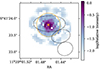 |
Fig. A.1. NIRSpec IFU PSF at 4μm as traced by the quasar Hβ broad-line flux. The location of the peak of the quasar is marked as an orange cross, with the 0 |

Appendix B: BPT diagnostics
Using our measured Hβ and [O III] λ5007 flux values and limits from Table 1, we place the emission-line regions on a BPT diagram (Baldwin et al. 1981), which we show in Figure B.1. This diagnostic aims to characterise the main photoionisation source based on the narrow-line flux; we use the fluxes measured from the quasar-subtracted cube, where the narrow-line flux is emitted by the extended galaxy component and the point source quasar contribution has been removed. As there are no existing measurements of [N II] λ6583 we can only constrain the location of these galaxies on the vertical [O III] λ5007/Hβ axis.
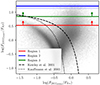 |
Fig. B.1. BPT diagnostic diagram showing the [O III] λ5007/Hβ flux ratio measured for the companion galaxy (Region 2), and the lower limits for the host galaxy (Region 1) and Region 3, as listed in Table 1. For reference, we show the Kauffmann et al. (2003) (black dotted) and Kewley et al. (2001) (black dashed) curves which attempt to differentiate between galaxies primarily ionised by star formation (lower left) and AGN (upper right) at low-z. We also show local sources from the SDSS (Abazajian et al. 2009, 2D histogram) for comparison. |
All Tables
Dynamical masses and values used in their calculation for the quasar host and companion galaxy.
Estimated BH masses (MBH), Eddington ratios (λEdd), and the FWHMs and luminosities used in their calculation for the quasar J1120+0641.
Extracted NIRCam magnitudes for the quasar host and companion galaxy, and their stellar mass (M*), fraction of stars formed in the recent starburst (fstarburst), and metallicity (Z) measured from the subsequent SED fitting.
All Figures
|
Fig. 1. Integrated spectrum of J1120+0641 from the IFU data (blue). The spectrum is integrated over an aperture of radius |
| In the text | |
|
Fig. 2. Quasar-subtracted [O III] λ5007 emission map from the NIRSpec IFU (grey image) compared to the [C II] 158 μm emission map (orange contours) and the rest-frame 158 μm FIR continuum emission map (purple contours) from ALMA (see Section 5.2). The [C II] 158 μm contours are linearly spaced from 5σ to 26σ, where σ = 16 μJy. The FIR continuum contours are linearly spaced from 5σ to 42σ, where σ = 7 μJy/beam. The grey circle depicts the approximate PSF of the ALMA observations, with beam diameter |
| In the text | |
|
Fig. 3. Emission-line regions surrounding J1120+0641 showing flux and kinematic maps after the subtraction of the quasar emission. The top-left and -right panels show the flux of the [O III] λ5007 and Hβ lines, respectively, from the integrated flux of the fitted Gaussian in each spaxel. The bottom-left and -right panels show our [O III] λ5007 kinematic maps, depicting the non-parametric central velocity of the line (v50) relative to the quasar host redshift of z = 7.0804 ± 0.0028 and the line width (w80), respectively. Three emission-line regions are highlighted by coloured ellipses, and the crosses show the location of the quasar. |
| In the text | |
|
Fig. 4. Quasar-subtracted spectra integrated over the three spatial regions shown in Figure 3 (opaque coloured lines) along with our best-fit Gaussian models for the Hβ and [O III] λλ4959,5007 emission lines (black). The analogous spectra from the non-quasar-subtracted cube are also plotted for comparison (transparent coloured lines), showing the necessity of quasar subtraction to accurately measure the emission from Regions 1 and 2. All spectra have been continuum subtracted. The vertical lines mark the location of the Hβ and [O III] λλ4959,5007 lines at the redshift of the quasar host galaxy, Region 1, as measured from the fit to this spectrum, z = 7.0804 ± 0.0028. For the host Region 1, we exclude the central 5 × 5 pixels surrounding the quasar peak as well as nearby spaxels with [O III] λ5007 velocity offset > 300 km/s, as these are highly corrupted by the quasar subtraction and introduce significant noise and artefacts. This means that we slightly underestimate the total flux in this region; however, the fluxes are significantly more reliable than if these most corrupted spaxels were included. |
| In the text | |
|
Fig. 5. Integrated quasar spectrum for J1120+0641 (black) showing the region around Hβ. The spectrum is integrated over a radius of |
| In the text | |
|
Fig. 6. Overlay plot of the F200W PSF-subtracted image (background image with colour bar) and the [O III] λ5007 map (white contour). The emission in the PSF-subtracted F200W image largely overlaps with the [O III] λ5007 line map, indicating that the continuum and line emission originate from the same objects, i.e. the quasar host and the close companion. The marked scale of 0 |
| In the text | |
|
Fig. 7. Results from the NIRCam PSF subtraction for J1120+0641. From left to right, the original NIRCam images, the PSF-subtracted images, the model for the host and the companion, the image fitting residual (i.e. the subtraction of the full model from the original image), the PSF-subtracted images divided by the error images, and the residual images divided by the error images. The extended emission is modelled as two Sérsic profiles using the positions and morphologies as measured from the [O III] λ5007 maps (Section 3.1). The PSF-subtracted images clearly show the extended emission around the quasar. |
| In the text | |
|
Fig. 8. Spectral energy distribution fitting for the host galaxy Region 1 (upper panels) and for the companion galaxy Region 2 (lower panels). The left and right columns correspond to a single delayed-τ SFH and a delayed-τ plus a starburst SFH, respectively. The red circles represent the NIRCam broad-band fluxes from image fitting, and the red triangles represent the observed Hβ and [O III] λλ4959,5007 line fluxes. The solid black line and the gray shaded region mark the Prospector modelled spectrum and its 1σ error, while the orange squares show the resulting model photometry. |
| In the text | |
|
Fig. 9. Black hole–stellar mass relation showing the overmassive BH in J1120+0641 (gold). Purple points show z ≳ 6 quasars with stellar mass estimates from JWST (Ding et al. 2023; Yue et al. 2024). Pink points show dynamical mass measurements for z ≃ 6 quasars as measured with JWST (Marshall et al. 2023), while grey points show dynamical mass measurements as measured with ALMA (Willott et al. 2017; Izumi et al. 2018, 2019; Pensabene et al. 2020). Blue points show measurements for high-z AGNs discovered with JWST (Maiolino et al. 2024; Harikane et al. 2023; Übler et al. 2023; Kokorev et al. 2023; Juodžbalis et al. 2024; Furtak et al. 2024; Napolitano et al. 2024). Green points show samples of low-z sources with large MBH/M* ratios (Mezcua et al. 2023; Trakhtenbrot et al. 2015; van den Bosch et al. 2012). The grey dashed lines depict MBH/M* ratios of 0.1%, 1%, 10%, and 100%. The coloured curves show the local Reines & Volonteri (2015) and Greene et al. (2020) relations, with the shaded regions showing the ±1σ scatter in the relations, for comparison. |
| In the text | |
|
Fig. A.1. NIRSpec IFU PSF at 4μm as traced by the quasar Hβ broad-line flux. The location of the peak of the quasar is marked as an orange cross, with the 0 |
| In the text | |
|
Fig. B.1. BPT diagnostic diagram showing the [O III] λ5007/Hβ flux ratio measured for the companion galaxy (Region 2), and the lower limits for the host galaxy (Region 1) and Region 3, as listed in Table 1. For reference, we show the Kauffmann et al. (2003) (black dotted) and Kewley et al. (2001) (black dashed) curves which attempt to differentiate between galaxies primarily ionised by star formation (lower left) and AGN (upper right) at low-z. We also show local sources from the SDSS (Abazajian et al. 2009, 2D histogram) for comparison. |
| In the text | |
Current usage metrics show cumulative count of Article Views (full-text article views including HTML views, PDF and ePub downloads, according to the available data) and Abstracts Views on Vision4Press platform.
Data correspond to usage on the plateform after 2015. The current usage metrics is available 48-96 hours after online publication and is updated daily on week days.
Initial download of the metrics may take a while.