| Issue |
A&A
Volume 702, October 2025
|
|
|---|---|---|
| Article Number | A59 | |
| Number of page(s) | 14 | |
| Section | Extragalactic astronomy | |
| DOI | https://doi.org/10.1051/0004-6361/202555465 | |
| Published online | 07 October 2025 | |
Globular clusters in M 104: Tracing kinematics and metallicities from the centre to the halo
1
Department of Astrophysics, University of Vienna, Türkenschanzstraße 17, 1180 Wien, Austria
2
Instituto de Astrofísica de Canarias, Calle Vía Láctea, E-38206 La Laguna, Spain
3
Departamento de Astrofísica, Universidad de La Laguna, E-38206 La Laguna, Spain
4
Centre for Astrophysics and Supercomputing, Swinburne University, John Street, Hawthorn VIC 3122, Australia
5
European Southern Observatory, Karl-Schwarzschild-Straße 2, 85748 Garching bei München, Germany
6
Department of Physics, Centre for Extragalactic Astronomy, Durham University, South Road, Durham DH1 3LE, UK
7
Institute of Physics, Laboratory of Astrophysics, Ecole Polytechnique Fédérale de Lausanne (EPFL), 1290 Sauverny, Switzerland
8
Institute of Astronomy, Madingley Rd, Cambridge CB3 0HA, UK
9
Visiting Fellow, Clare Hall, University of Cambridge, Cambridge, UK
10
Instituto de Física, Universidade Federal do Rio Grande do Sul (UFRGS), Av. Bento Gonçalves, 9500, Porto Alegre RS 91501-970, Brazil
⋆ Corresponding author: This email address is being protected from spambots. You need JavaScript enabled to view it.
Received:
9
May
2025
Accepted:
12
August
2025
Abstract
As ancient star clusters, globular clusters (GCs) are regarded as powerful tracers of galaxy evolution and assembly. Due to their brightness and compact sizes, GCs are employed to probe the kinematics and stellar population properties of galaxies, from the central regions out into the halo where the underlying stellar light becomes too faint for spectroscopic studies. In this work, we present a comprehensive study of the GC system of M 104 (NGC 4594, also known as the Sombrero galaxy) based on literature spectroscopic catalogues and newly collected data from Very Large Telescope (VLT) MUSE integral-field spectroscopy combined with multi-object spectroscopy from VLT FLAMES and OSIRIS at the Gran Telescopio de Canarias (GTC). We present a new catalogue of 499 GCs with radial velocity measurements that span from the inner disc region out to ∼70 kpc (24′). In addition to velocities, we measured metallicities from the MUSE, OSIRIS, and FLAMES spectra of 190 GCs. Together with literature values, we collected a sample of 278 metallicities. We found good agreement between the velocity and metallicity measurements of GCs observed with multiple instruments. Studying GC kinematics with a simple model confirms a decreasing velocity dispersion profile and low rotation velocities. The blue GCs appear to be more dispersion-dominated, while the red GCs follow the kinematics of the stars more closely. We find a large scatter of GC metallicities with distance from the centre, and metal-rich GCs are found over all radii. We discuss how the GC metallicity distribution with a broad metal-poor component likely reflects the complex assembly history of M 104.
Key words: galaxies: individual: M 104 / galaxies: star clusters: general
© The Authors 2025
 Open Access article, published by EDP Sciences, under the terms of the Creative Commons Attribution License (https://creativecommons.org/licenses/by/4.0), which permits unrestricted use, distribution, and reproduction in any medium, provided the original work is properly cited.
This article is published in open access under the Subscribe to Open model. This email address is being protected from spambots. You need JavaScript enabled to view it. to support open access publication.
1. Introduction
As ancient star clusters with typical ages well above 10 Gyr, globular clusters (GCs) have long been regarded as powerful tracers of galaxy formation and assembly (see Forbes et al. 2018 or Beasley 2020 for reviews). With their masses on the higher end of the stellar cluster population (104–106 M⊙) and compact sizes (Reff ∼ 3 pc), GCs are observable in the halo regions of distant galaxies. High-quality photometric GC catalogues from space-based imaging or multi-band ground-based observations are available for hundreds of galaxies (e.g. Le & Cooper 2025; Lim et al. 2025), providing luminosities, sizes, and colours for thousands of GCs (see Jordán et al. 2007; Harris et al. 2013, 2017). Complementary spectroscopy is required to use GCs as tracers of galaxy properties and mass assembly since it enables measurement of line-of-sight (LOS) velocities and stellar population properties such as metallicities or light element abundances (e.g. Pota et al. 2013; Forbes et al. 2017; Chaturvedi et al. 2022).
In this paper, we revisit the GC system of M 104 (NGC 4594), also known as the Sombrero galaxy. At a distance of D = 9.55 ± 0.13 ± 0.31 Mpc (McQuinn et al. 2016), M 104 has been studied extensively due to its peculiar morphology with a nearly edge-on orientation and prominent dust lane (Emsellem 1995; Sutter & Fadda 2022). M 104 is traditionally classified as an Sa galaxy; however given its prominent spheroidal component (Gadotti & Sánchez-Janssen 2012), metal-rich halo (Cohen et al. 2020), and high specific frequency of GCs (SN ∼ 2; Rhode & Zepf 2004; Kang et al. 2022), there is growing evidence that M 104 is a lenticular early-type galaxy (see Kang et al. 2022). With a stellar mass of M* ∼ 2 × 10¹¹ M⊙ (Jardel et al. 2011; Karachentsev et al. 2020), it is the brightest and most massive member of its group. Based on radial velocities of dwarf galaxies, the total mass of the group is Mtot = (1.24 ± 0.65)×1013 M⊙ (Crosby et al. 2025).
The rich GC system of M 104 has been extensively studied for many decades using both imaging and spectroscopy (e.g. Wakamatsu 1977; Harris et al. 1984; Bridges & Hanes 1992; Bridges et al. 1997, 2007; Forbes et al. 1997). The total number of GCs is estimated to be around 1500–2000 (Harris et al. 1984; Rhode & Zepf 2004; Kang et al. 2022), which is about an order of magnitude more than the number of GCs around the Milky Way or M 31. The GC colour distribution of M 104 was found to be bimodal, with a large fraction of red metal-rich GCs (Larsen et al. 2001, 2002; Alves-Brito et al. 2011). In 2003, M 104 was observed with multiple pointings of the Advanced Camera for Surveys (ACS) on board the Hubble Space Telescope (HST), enabling a 600″ × 400″ mosaic to be constructed. In these data, 659 GCs were identified (Spitler et al. 2006), and Harris et al. (2010) presented updated photometry and size measurements for 652 GCs in the inner region of M 104. More recently, Kang et al. (2022) used ground-based imaging with the MegaCam instrument at the Canada-France-Hawaii Telescope and presented a catalogue of ∼2900 candidates out to 35′ (∼100 kpc). They estimated a total number of GCs of 1610 ± 30 based on the number of candidates above the turn-over magnitude.
The most recent spectroscopic catalogue of GCs around the Sombrero galaxy was compiled by Dowell et al. (2014). They combined their own observations of 51 GCs with the sample of 108 GCs from Bridges et al. (2007) and the catalogue of 259 sources from Alves-Brito et al. (2011). The catalogue of Dowell et al. (2014) lists 579 unique sources, about 360 of them are confirmed GCs of M 104 based on their radial velocities.
In this paper, we aim to build on the above mentioned works to present the largest catalogue of spectroscopically confirmed GCs around the Sombrero galaxy to date. Combining the literature compilation from Dowell et al. (2014) with new observations from the Multi Unit Spectroscopic Explorer (MUSE; Bacon et al. 2014) instrument at the Very Large Telescope (VLT), the Fibre Large Array Multi Element Spectrograph (FLAMES; Pasquini et al. 2002) instrument at the VLT, and the Optical System for Imaging and low-Intermediate-Resolution Integrated Spectroscopy (OSIRIS; Cepa 1998) instrument at the Gran Telescopio Canarias (GTC), we report on a catalogue of 499 GCs. Section 2 describes those datasets, and we present our analysis methods in Sect. 3. Results are presented and discussed in Sect. 5. We conclude in Sect. 6.
2. Data
In this work, we collected a new large sample of spectroscopically confirmed GCs using MUSE integral field spectroscopic data, FLAMES high resolution multi-object spectroscopy, and deep OSIRIS multi-object spectroscopy of bright GCs. This section describes the data reduction methods and Fig. 1 shows the observation footprints.
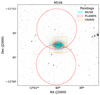 |
Fig. 1. Footprints of the different datasets on a greyscale DSS2 image of M 104. MUSE pointings are shown in cyan squares, each with a field of view of 1′×1′. The red circles indicate the field of view of the FLAMES GIRAFFE instrument, with a diameter of 25′, and the orange rectangles show the field of view of OSIRIS, which spans 7.5′×6′. The full greyscale image is 40′ × 40′ (110 kpc × 110 kpc). |
2.1. MUSE data
M 104 was observed with MUSE as part of the science verification run (programme ID 60.A-9303, PI: Emsellem) in 2014 after MUSE was commissioned at the VLT. The MUSE data consist of 15 unique pointing positions covered by two exposures each along the disc as well as above and below around the central part of M 104. The exposure time varies between 210 and 600 seconds per exposure, with shorter exposure times on the bright galaxy centre. The total exposure times increase outwards with the central exposure cumulating 420 seconds, while the two surroundings disc fields have 600 seconds. The next set of 8 fields (in the disc and off-plane) have 900 seconds, while the 4 most outer pointings have 1200 seconds. The average seeing was 1.2″, with some exposures reaching 0.45″ and others > 2.0″.
All data were reduced following a standard process and making use of python scripts wrapping around ESOREX commands and the Data Reduction Software developed by the MUSE consortium (Weilbacher et al. 2020). The relative alignment of individual exposure was performed using the reference HST F625W mosaic. Individual dedicated sky pointings were used to remove the background contribution after renormalisation of the derived sky spectrum. The final MUSE mosaic was assembled using the ESOREX MUSE_EXP_COMBINE command. We only considered the bluer part of the data cube up to 7400 Å due to stronger sky residuals at longer wavelengths. The spectra are sampled at 1.25 Å pix−1 and with an instrumental resolution of ∼2.5 Å.
To detect the spectra of GCs in the MUSE data, we followed the methods described in Fahrion et al. (2020). As first step, we created a white light image using the median of 1000 wavelength slices from the MUSE data cube. Then, the bright galaxy background was removed using a median filter based on PHOTUTILS’ background subtraction functions. We chose a box size of 5 × 5 pixels with a filtersize of 3 × 3 pixels. In the background subtracted image, all sources 2σ above the background rms were detected using PHOTUTILS SEGMENTATION detection routines with a FWHM of 4 pixels. To remove resolved background galaxies, only sources with eccentricity < 0.7 were kept, yielding 488 initial sources.
In the second step, we extracted the spectra of those sources using a Gaussian-weighted aperture with a FWHM of 4 pixels (0.8″). We also tested other values, but found that the influence on the final spectrum is minimal. For each source, a background spectrum was extracted using an annulus with inner radius of 8 (1.6″) and outer radius of 13 pixels (2.6″). Subtracting the background spectrum, we obtained 258 GC candidates with signal-to-noise (S/N) > 2.5 pix−1, as derived from the ESTIMATESNR function of PYASTRONOMY (Czesla et al. 2019) in a wavelength region between 6400 and 6500 Å. Of those, 139 sources could be matched to the photometric GC catalogue of Harris et al. (2010) based on HST data. In the last step, the spectra were fitted with PPXF as described in Sect. 3.1 to confirm membership to M 104.
2.2. FLAMES data
The extensive GC system of M 104 was observed with FLAMES GIRAFFE in MEDUSA mode (multi-object spectroscopy, programme ID 114.274W, PI: Fahrion) in January and February 2025 in two pointings, one to the north of the disc and one to the south. Each pointing has a diameter of 25′ and the FLAMES fibers were placed on 221 GC candidates derived from the HST catalogues (Spitler et al. 2006; Harris et al. 2010) and the catalogue from Kang et al. (2022) based on ground-based imaging. Additionally, 12 fibers were placed on empty sky regions. The HR21 (875 nm) grating was used, which provides coverage of the calcium triplet region from 8483 to 8900 Å at a resolution of R = 18 000 with a sampling of 0.05 Å pix−1. Each pointing was covered in ten exposures of 1365 seconds each, distributed over five observing blocks.
The FLAMES data were reduced using a custom wrapper around the data reduction scripts of the FLAMES ESOREX pipeline1. We followed mainly the standard processing steps according to the manual, including bias and flat fielding corrections, followed by a wavelength calibration. As recommended in the manual, we ran the wavelength calibration twice to obtain a custom slit geometry table and an improved wavelength solution. Afterwards, the science reduction is completed for each exposure. We chose the extraction method ‘OPTIMAL’, which gives an improved spectral extraction (Horne 1986).
In a second step of the data reduction, the sky was subtracted. In the ESOREFLEX pipeline, a master sky is created from all sky fibers and then subtracted. For bright sources, this approach is sufficient, but we chose to implement an improved approach to further reduce residuals for also fainter objects. Individual sky fibers were used to create a library of sky templates for each exposure. Then, we used the penalized pixel fitting method (PPXF; Cappellari & Emsellem 2004; Cappellari 2017, 2023), a full spectrum fitting method to fit spectra with user-supplied models, to fit each spectrum with a stellar model from the PHOENIX library (Husser et al. 2013) and the sky templates as sky input. The PHOENIX models give synthetic stellar atmosphere spectra, provided at a spectral resolution of R = 500 000, which we brought to the FLAMES resolution by convolution with a Gaussian. The full library covers a large range of stellar parameters, but we selected red giant stars with effective temperature between 4500 and 5000 K, surface gravity between log(g) = 2.0 and 4.0, and a range of metallicities between –1.5 and 0 dex. We note here that we only used the PHOENIX stellar spectra for the sky subtraction and did not consider the fits further. The best-fitting combination of sky templates are then subtracted and the spectra are saved. Compared with the master sky subtraction approach, the fitting with PPXF allows us to accurately scale the sky spectra and further reduce the sky line residuals. In addition to the sky subtraction, we also used the sky observations to measure the spectral resolution. For this, we fitted the strong sky lines in each sky fiber of each exposure, testing if the spectral resolution is stable across exposure and fibers. As also described in Beasley et al. (2025), we did not find a trend with wavelength or exposure. The median FWHM of the sky lines is 0.54 ± 0.04 Å across the different exposures.
In the final step of the data reduction, the exposures for each individual source were combined, accounting for the barycentric velocity of each exposure and resampling all spectra on a common wavelength array. To get an improved combination, we used a median, weighted by the S/N in each exposure. We also kept a version of the spectra without sky subtraction and used those to mask regions of strong sky contamination in the fits (see Sect. 3.3)
2.3. GTC data
75 GCs of M 104 were observed with the GTC using the OSIRIS instrument in multi-object spectroscopy mode (programme IDs GTC24-19A, GTC89-20A, PI: Beasley). Three fields were covered (Field 2: RA: 12:39:52.31, Dec: –11:35:15.7; Field 3 : RA: 12:40:06.02, Dec: –11:39:07.5; Field 4: RA: 12:39:52.16, Dec: –11:38:59.8; J2000), using exposure times of 3–3.75 hours in 900 s individual exposures. Targets were selected from the HST ACS catalogue of Spitler et al. (2006) augmented with candidates from Rhode & Zepf (2004). The R1000B grating was used with a 0.6″ slit, giving a wavelength range of 3700–7500 Å and spectral resolution with a FWHM of ∼5 Å.
Data were reduced using the GTC OSIRIS spectrograph package implemented in PYPEIT2 (Prochaska et al. 2020a,b). Standard data reduction procedures were followed, and the individual spectra were wavelength calibrated (in vacuum wavelengths), optimally extracted, corrected to the barycentric frame, and combined. The one dimensional spectra were flux- and extinction calibrated based on long-slit observations of the standard star HD289002 (Hiltner 600) observed in the same setup but with a 1.0″ slit. We note that the flux calibration applied is only approximate – mainly to correct the continuum shape – due to the problem of precise calibrations of multi-slit spectra. The final S/N ratio of the spectra are high, with median S/N = 74 pix−1.
3. Spectroscopic analysis
We fit all GC spectra with PPXF and tested different models. Figure 2 shows the MUSE, OSIRIS, and FLAMES spectra a GC for which spectra from all three instruments are available as illustration of the different datasets. In this figure, the different spectral resolutions becomes evident, as well as the imperfect flux calibration of the OSIRIS spectra.
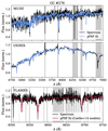 |
Fig. 2. Spectra of GC #276 for which spectra from MUSE (top), OSIRIS (middle), and FLAMES (bottom) are available. The black lines show the data, and the blue and red lines are the fits with PPXF. Shaded regions were excluded due to sky line residuals. The MUSE and OSIRIS spectra were fitted with XSL SSPs, while we used high resolution stellar models from Coelho (2014) to fit the FLAMES spectrum shown here. |
3.1. Fitting MUSE spectra
For fitting the MUSE spectra, we used the E-MILES3 single stellar population (SSP) models (Vazdekis et al. 2010, 2016). Those are SSP models based on the empirical MILES stellar spectra, combined with BaSTI isochrones (Pietrinferni et al. 2004, 2006) and a double power-law initial mass function with a high mass slope of 1.30 (Vazdekis et al. 1996). The models span an age range between 30 Myr and 14 Gyr and have total metallicities between [M/H] = –2.27 dex and +0.40 dex. For comparison purposes, we also fitted the spectra with SSPs based on the X-Shooter spectral library (XSL)4 presented in Verro et al. (2022). We chose the models based on the PARSEC/COLIBRI isochrones (Bressan et al. 2012; Marigo et al. 2013; Chen et al. 2015) using the initial mass function from Kroupa (2001). The models have ages above 50 Myr, and iron metallicities between [Fe/H] = –2.2 and +0.2 dex.
While the E-MILES models reach up to [M/H] = +0.4 dex, the XSL SSPs give models up to [Fe/H] = +0.2 dex, which artificially decreases the metallicities derived from the XSL models at high metallicities. Additional differences might be caused by light element abundances. The E-MILES models assume [M/H] = [Fe/H]; however, this is only strictly true at high metallicities due to empirical MILES spectra that were used to construct the models that follow the abundance pattern of the solar neighbourhood. The E-MILES models are sampled at 1.25 Å pix−1 with a spectral resolution of 2.5 Å, while the XSL SSPs have a resolution of R ∼ 10 000 (σ = 16 km s−1). When fitting MUSE spectra, we considered the wavelength-dependent line spread function description from Guérou et al. (2017).
When fitting the GC candidate spectra, we took a two step approach. Firstly, we fitted for the LOS velocities using additive polynomials of degree 12. Then, all candidates with S/N > 7.5 were fitted with fixed velocities and no additive polynomials. Multiplicative polynomials of degree 8 were used to minimise template mismatch. As PPXF returns the weights of the best-fitting combination of models, we can reconstruct the best-fitting age and metallicity from the fit. Sky residual lines were masked and we only considered the wavelength range between 4700 and 7100 Å. While we left the velocity dispersion as a free parameter in the fitting, we did not attempt to constrain it as the expected velocity dispersions of GCs (< 20 km s−1) is significantly lower than the MUSE instrumental resolution (∼80 km s−1).
After performing initial fits for all 258 GC candidates from the MUSE data, we inspected the fits and removed obvious contaminants such as foreground stars and background galaxies from the sample. The remaining 179 spectra are then fitted again with a Monte Carlo (MC) approach to derive statistical uncertainties on the parameters. Here, the best-fitting spectrum is perturbed using the residual of the initial fit to randomly draw noise in each wavelength. This creates 100 realisations of the spectrum that are then fitted to obtain distributions of the velocity, age, and metallicity. The reported values refer to the mean and standard deviation of the fits. To speed up the fitting procedure, we restricted the model library to SSPs with ages > 5 Gyr, as we do not see any indication of younger ages from the initial fits.
Of the full sample, we kept 152 GC candidates that have velocity uncertainties < 100 km s−1, 114 of them are matched to the HST catalogues. Of those, 126 have uncertainties < 50 km s−1 (98 matched to HST). Most of the GCs without a match to the HST catalogues are in the disc region M 104 and might therefore be clumps embedded in the dust lanes rather than genuine GCs. To remove those, we inspected all GCs without match to the HST catalogue (Harris 2010) on the HST colour image and kept only those with clear cluster-like morphology. This leaves us with a final sample of GCs with MUSE spectra of 139 GCs with velocity uncertainties lower than 100 km s−1 (118 with uncertainties smaller than 50 km s−1). The MUSE sample is shown in Fig. 3 on top of a white-light image of the MUSE data. We discuss the completeness of the MUSE sample in Appendix A.
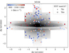 |
Fig. 3. Distribution of GCs extracted from MUSE data. Individual GCs are marked with dots colour-coded according to their LOS velocity. Small dots are GC candidates without match to the HST catalogue from Spitler et al. (2006) and Harris et al. (2010). The greyscale image shows the white light image from MUSE. |
In addition to the GCs, we also used the MUSE data to investigate the stellar light of M 104. We binned the data cube using a Voronoi binning scheme with the VORBIN package (Cappellari & Copin 2003) to a signal-to-noise of 300, resulting in 626 bins. Those binned spectra were fitted with the same PPXF setup to obtain velocities, velocity dispersions, and stellar population properties. While a full analysis of the stellar component of M 104 is beyond the scope of this work, we used these properties for comparison against the GC sample.
3.2. Fitting OSIRIS spectra
To fit the GTC/OSIRIS spectra, we chose the same setup for PPXF as for the MUSE spectra, except for adapting the E-MILES and XSL SSP models to the OSIRIS resolution of FWHM = ∼5 Å. Due to the decreasing sensitivity in the blue and prominence of sky line residuals in the red, we chose a wavelength range between 4550 and 7100 Å. Before fitting the GTC spectra, we rebinned them to a common wavelength array with a sampling of 2.0 Å.
As for the MUSE spectra, we first fitted all spectra and then did a visual inspection of the fits to remove five low S/N spectra and one background galaxy. In a second step, we used an MC approach to derive mean velocities, ages, and metallicities for a final sample of 69 GCs.
3.3. Fitting FLAMES spectra
Due to the significantly higher spectral resolution of FLAMES, we used the stellar atmosphere models from Coelho (2014)5 to obtain radial velocities with PPXF. Those models have a sampling of 0.02 Å pix−1 at a spectral resolution of R = 20 000, which we match to the FLAMES resolution (FWHM = 0.54 Å) by convolution with a Gaussian kernel. To fit the velocities of GCs, which are dominated by the light from red giant branch stars in the wavelength range of the FLAMES spectra, we selected stars with 4000 < Teff < 5000 and 0.5 < log(g) < 3. Velocity dispersions obtained from the high resolution FLAMES spectra will be presented in a future work.
Similar to the other datasets, we first fitted all FLAMES spectra to obtain initial estimates of the LOS velocities. Then, we removed those sources with velocities < 200 km s−1, which are foreground stars rather than GCs belonging to M 104, and those that did not show absorption lines in the spectrum, leaving 110 GCs. In the second step, we performed MC fitting with 100 iterations to obtain statistical uncertainties on the velocities. Due to the high resolution of FLAMES, we found typical velocity uncertainties of the order of 0.5–2 km s−1.
To measure metallicities from the FLAMES spectra, we also fit the spectra with the XSL and E-MILES SSP models. Due to the lower spectral resolution of the models compared with the data, we convolved the FLAMES spectra to match that of the models, and then repeated the fitting to obtain also metallicities in a similar approach as for the MUSE and OSIRIS spectra. We restricted the SSPs to ages > 10 Gyr to limit the age-metallicity degeneracy. As the calcium triplet is rather insensitive to age (e.g. Sakari & Wallerstein 2016), we do not expect that this impacts our results, also because there are no indications of young ages from the MUSE or OSIRIS GCs.
4. Catalogue of GCs around the Sombrero galaxy
In this section, we describe the final GC samples from the different datasets and compare their velocities and metallicities. The final catalogue is then also described in Appendix D.
4.1. Removing contaminants
Collecting the objects with successful fits from MUSE, OSIRIS, and FLAMES results in 302 sources. Together with the full catalogue of 579 sources from Dowell et al. (2014), we have collected 881 radial velocity measurements of objects around M 104. Before removing contaminants such as foreground stars and unbound GCs, we cross-matched the different catalogues to identify duplicates. Using a matching radius of 1″, we could identify 721 unique sources. Figure 4 shows the LOS velocities of these sources as a function of the projected distance from the galaxy centre. In case a source is contained in more than one of the samples, we show here the velocity with the smallest uncertainty. As shown in Sect. 4.2, the velocities between the different samples agree.
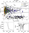 |
Fig. 4. Outlier removal based on GC velocities and projected distances. Top: Line-of-sight velocities as a function of projected galactocentric distance for the full sample of 721 unique sources. Different colours refer to different samples. In case a source is found in multiple samples, only the velocity with the smallest uncertainty is shown. Bottom: Difference between mN and mN − 1 as a function of GC number N (left, see Eq. (1)) and the derivative (right). The vertical grey line indicates our chosen cut-off Ncut = 222, right after the last big jump as seen in the derivative. From this value, the corresponding vmax(R) curve was derived, which is shown as the grey dashed line in the top panel. The shaded regions show the curves when assuming Ncut ± 5. |
Overview of GC samples.
As can be seen in Fig. 4, the samples span over different regions, with the MUSE sample tracing the innermost GCs and the FLAMES sample reaching out to 20′. While we already removed obvious contaminants such as background galaxies and foreground stars with v < 200 km s−1, Fig. 4 shows that there is a population of foreground stars, as also described in Dowell et al. (2014), with small LOS velocities, as well as possible intra-group GCs with high velocities.
To remove contaminants from the sample, we followed the approach described in Dowell et al. (2014), which is based on the method from Schuberth et al. (2010, 2012). The approach is based on a tracer mass estimator from Evans et al. (2003) that can be applied when the distribution of tracers is different from the overall mass distribution, as for the case of GCs. For this, the quantity mN of N GCs is calculated as
 (1)
(1)
where vi and Ri are the velocity relative to the systemic velocity and projected radius of the ith GC. We assume here a systemic velocity of 1089.1 km s−1 as derived by Sutter & Fadda (2022) from the MUSE data. We verified this velocity with our binned stellar kinematic analysis. mN is proportional to the tracer mass estimate, but if all GCs including outliers are considered, this estimate is very large. Therefore, to probe where the tracer mass estimates starts to converge, the source with the largest vi2Ri is removed from the sample and mN is recomputed. This is repeated for all objects, and since the GCs belonging to M 104 should trace the same underlying mass, mN should converge when all outliers are removed. Consequently, the cut-off value Ncut is identified as the point when the curve mN–mN − 1 as a function of N begins to flatten (Fig. 4). As this choice is somewhat subjective, we followed here Dowell et al. (2014) and Schuberth et al. (2010), and set Ncut as the point after the last large jump in the mN–mN − 1 curve. This jump was identified from the derivative (bottom right panel in Fig. 8). We used Ncut = 222 to balance between removing clear outliers and still retaining a large GC sample. Other choices that are within Ncut = 222 ± 5 also seem reasonable, but for lower values, some of the foreground stars would be kept in the sample, and for higher values of Ncut, GCs would be removed.
In the last step of the outlier removal, Cmax = vNcut + 12RNcut + 1, is derived as the v2R value of the first non-removed GC. Based on this, the  curve is obtained to select the final GC sample (dashed line in the top panel of Fig. 4). Using this selection, we obtained a sample of 499 GCs, which we use in the following. We note that a different choice for Ncut does not alter the results significantly. Compared to the estimated total number of GCs (1500–2000, Rhode & Zepf 2004; Kang et al. 2022), this constitutes a significant fraction (∼25 − 30%) of all GCs.
To visualise this sample, we show the distribution of 499 GC velocities and 278 metallicities (190 of those were not yet reported in Alves-Brito et al. 2011) in Fig. 5. In Appendix B, we show a zoom into the central 5″ × 5″. Due to the two FLAMES pointings north and south of the disc, the distribution is asymmetric, but reaches out to ∼25′ from the centre of M 104. In addition to GCs, we also added the coordinates of dwarf galaxy candidates near M 104 marked as crosses (Crosby et al. 2024). Interestingly, one GC from the Dowell et al. (2014) catalogue can be associated with the dwarf galaxy dw1239-1143. Inspecting the imaging presented in Crosby et al. (2024) of this dwarf suggests that the corresponding GC is the nuclear star cluster of this dwarf. Additionally, we note that we covered SUCD1 (Hau et al. 2009), an ultra-compact dwarf (UCD) galaxy in our sample with a FLAMES spectrum. As discussed in Hau et al. (2009), this object has similar properties as other UCDs or massive GCs. They discussed that its elevated velocity dispersion and brightness might indicate that it is the remnant nucleus of a disrupted dwarf galaxy rather than a dwarf galaxy itself. This interpretation might also be supported by the discovery of a stellar stream around M 104 that could be connected to this UCD (Martínez-Delgado et al. 2021).
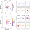 |
Fig. 5. Spatial distribution of GC velocities (top) and metallicities (bottom). The large panels on the left show the full distribution of velocities and metallicities, respectively. Circles refer to this work; triangles refer to GCs listed in the Dowell et al. (2014) and Alves-Brito et al. (2011). Black crosses show dwarf galaxy candidates near M 104 from Crosby et al. (2024). The smaller panels on the right side show the velocities and metallicities in different bins, as indicated in the panel titles. Fig. B.1 shows a zoom-in of the central 5′ × 5′. |
Inspecting the spatial distributions of velocities and metallicities in Fig. 5, we see that GCs with more extreme relative velocities tend to be centrally concentrated. This is a direct effect of the gravitational potential of M 104, which dictates the escape velocity, as also visible in the declining vmax(R) curve in Fig. 4. While overall, no clear rotation signature is visible, there might be a trend of higher relative velocities to the east side of the centre than to the west within the inner ∼3′, which would follow the rotation of the disc. The most metal-rich GCs are found close to the centre, while lower metallicities dominate at larger separations, as is further discussed in Sect. 5. A small population of extremely metal-poor GCs with [M/H] < − 2 dex is found to be also centrally concentrated, but the low numbers hinder any conclusion about their spatial distribution.
4.2. Comparing GC samples
In the final sample of 499 GCs, 365 were listed by Dowell et al. (2014), 139 have velocities from MUSE, 94 from FLAMES, and 69 from OSIRIS. Table 1 gives an overview of the different samples, including the numbers, median velocity uncertainties, and S/N values. As can be seen, the high resolution FLAMES spectra give by far the most precise velocity measurements. Due to the large field of view of FLAMES, this sample also probes the largest galactocentric distances, whereas MUSE allowed us to probe the central regions.
In Fig. 6, we compare the velocities of the different samples using the GCs that are listed in more than one catalogue. The large dots in the figure refer to GCs with velocity uncertainties < 20 km s−1 in the corresponding catalogues and we use those to test whether there are significant offsets between the samples using paired t-tests. The p-values are reported in the bottom left corners of the panels in Fig. 6. We find no significant offsets with p-values > 0.05 in most cases, except when comparing the catalogue from Dowell et al. (2014) with MUSE and when comparing FLAMES and OSIRIS measurements. In the latter case, the comparison is only based on a few GCs with a large scatter in the velocity differences, which makes it difficult to assess if there is a systematic offset, especially since the two instruments have very different velocity resolutions. The mean difference between the MUSE and the matched velocities from Dowell et al. (2014) is ⟨vDowell+14 − vMUSE⟩ = 15.2 km s−1 with a standard error of the mean of 5.9 km s−1. We chose not to apply this offset because the comparisons between the heterogenous Dowell et al. (2014) sample and velocities from FLAMES and OSIRIS do not show a similar consistent offset. Additionally, the few matches between MUSE and FLAMES show a very good agreement (⟨vMUSE − vFLAMES⟩ = 3.0 km s−1 with a standard error of 2.5 km s−1). However, we note that applying such an offset to the MUSE velocities (or the velocities from Dowell et al. 2014) does not significantly affect our results.
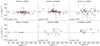 |
Fig. 6. Comparison of LOS velocities. Black dots are all the GCs found in both samples as indicated by the titles of the panels. Large pink circles are GCs where the velocity uncertainty in both samples is less than 20 km s−1. In the bottom-left corner, we report the p-value of a paired t-test. |
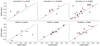 |
Fig. 7. Comparison of GC metallicities. The first sample reference in the panel title refers to the x-axis and the second to the y-axis. The grey dashed line is the one-to-one relation. We note that the literature metallicities from Alves-Brito et al. (2011) refer to iron metallicities, while we show here the total metallicities inferred from the E-MILES SSP models. |
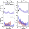 |
Fig. 8. Results of the simple kinematic model as a function of radius. Top left: GC system rotation amplitude vrot for all GCs in purple. The black line shows the LOS velocities of the stellar component, taken along a slit 0.4′ above the plane of the disc. Top right: Velocity dispersion of the full GC sample σGCS in purple. Within the rotation-dominated disc, the dispersion is significantly lower than off-plane. Bottom panels: GC rotation amplitude and dispersion for the red and blue GC subpopulations, separately. |
4.3. Comparing metallicities
In Fig. 7, we compare the metallicities of GCs listed in at least two of the samples. For the MUSE and OSIRIS samples, we used here the total metallicities as obtained with the E-MILES SSP models. As a literature comparison, we used the mean metallicities from Alves-Brito et al. (2011), who used line index measurements to estimate iron metallicities. While there can be differences between iron and total metallicities, for example depending on the light element abundance ratio, we show in Appendix C that the iron metallicities obtained when fitting with the XSL SSPs agree very well with the total metallicities from the E-MILES models. However, as the XSL SSPs only reach up to +0.2 dex, we chose to use the total metallicities from the E-MILES SSPs, as many of the GCs reach high metallicities.
Overall, the metallicities obtained here agree reasonably well with the results from Alves-Brito et al. (2011), even though we used full spectrum fitting. In addition, the metallicities from the different instruments (MUSE, FLAMES, OSIRIS), also agree with each other. The best match is found between the MUSE and OSIRIS metallicities, which is expected because both instruments cover the same optical wavelength range and the same fitting approach was taken. Interestingly, also the metallicities obtained from fitting the narrow calcium triplet region of the FLAMES spectra agree with the optical measurements, as especially the comparison between FLAMES and OSIRIS metallicities shows. While there seems to be indications that the metallicities from FLAMES might saturate at the highest metallicities ([M/H] > 0 dex, see also Usher et al. 2015; Sakari & Wallerstein 2016; Chung et al. 2016), this is encouraging because it allowed us to trust the FLAMES metallicities at larger galactocentric distances, where no optical spectra are available and GC metallicities are expected to be lower than in the central region (see Sect. 5.2).
5. Kinematics and metallicities of the GC system of M 104
In the following section, we use our collected catalogue of GC velocities and metallicities for an initial exploration of M 104’s GC system. We focus on a simple kinematic model describing the rotation and velocity dispersion of the GC system and investigate the GC metallicity distribution of M 104.
5.1. Simple kinematic model
We modelled the kinematics of the GC system with a simple sinusoidal model to constrain the rotation and velocity dispersion of the GC system as a function of radius from the galaxy centre. We followed the approach described in Fahrion et al. (2020, 2025), which is similar to the method described in Dowell et al. (2014) for M 104. In this sinusoidal model, the rotation of the GC system is described as
 (2)
(2)
where vrot describes the rotation amplitude around the systemic velocity vsys with θ0 denoting the angle of the rotation axis (maximum rotation is found at θ0 + 90°). vGC,i is the velocity of the ith GC at position angle θi, which is used as input to the model. In this model, only the global rotation and dispersion is considered, and any change with radius has to be implemented by choosing GCs at different radii.
The likelihood function is then given as
 (3)
(3)
where σobs2 = (δvGC,i)2 + (σGCS)2 describes the velocity dispersion σGCS under the assumption that the observed dispersion has contributions from the intrinsic GC system dispersion and the velocity uncertainty δvGC,i of the ith GC.
We used the python module EMCEE6 (Foreman-Mackey et al. 2013) to implement the model using a Markov chain Monte Carlo sampler in a Bayesian framework. As described in Sect. 4.1, we used the value with the lowest velocity uncertainty for GCs listed in two or more of the samples. When modelling the full GC system using all 499 GC velocities, we used flat priors on all parameters. For the rotation amplitude, we allowed positive values up to 400 km s−1 and constrained the position angle between −180° and 180°. The velocity dispersion prior ranges between 0 and 500 km s−1 and for the systemic velocity, we used a range between 800 and 1500 km s−1. For the full GC system, we find a dispersion of  km s−1, a low rotation amplitude of
  km s−1, a position angle of
  degrees, and a systemic velocity of
  km s−1, very similar to the systemic velocity of the galaxy as reported in Sutter & Fadda (2022) based optical emission lines in the MUSE data.
Due to the large number of GCs available, we were able to constrain the parameters at different radii, choosing radial bins out to 18′. The resulting profiles of rotation amplitude and dispersion are shown in the top panel of Fig. 8. We fixed the systemic velocity to the systemic velocity of the galaxy (vsys = 1089.1 km s−1, Sutter & Fadda 2022) to avoid effects from the inhomogeneous spatial coverage of the velocity measurements at larger radii. For the same reason, we also constrained the position angle with a Gaussian prior using a mean of 0° and a standard deviation of 10° to fix the angle of maximum rotation to a similar angle as the disc (∼90°).
In addition to fitting the full sample of GCs, we separated them into blue and red GCs. For GCs with B, V, and R magnitudes available (from Rhode & Zepf 2004 and Harris et al. 2010), we used a separation in colour of B − V = 0.8 mag. For GCs with g − i colours from Kang et al. (2022), we used a separation of g − i = 1.0 mag. We adapted the radial bins to ensure that at least ten GCs are in each radial bin. The rotation velocity and dispersion of the red and blue GC subpopulations are shown in the bottom panels of Fig. 8.
Similar to Dowell et al. (2014), we find low rotation velocities except for the innermost bin (< 1′) where the rotation velocity reaches above 100 km s−1. To compare this with the stellar component, we took an average LOS velocity profile along a slit 0.4′ above the disc shown as the black line in the top left panel of Fig. 8. We find that the disc itself reaches velocities ±350 km s−1 at low velocity dispersions of σ* ∼ 60 km s−1 (see also Sutter & Fadda 2022 for a description of the gas kinematics within the disc), so this off-plane slit was chosen to trace the spheroid component of M 104. In this central, off-plane region covered by the MUSE data, the stars show also high dispersions between 200–250 km s−1, while the GCs show even higher dispersions of  km s−1. At larger radii, the GC system velocity dispersion drops to
  km s−1 in the outermost bin (10 < R < 30′, ∼42 kpc).
Using the LOS velocities of nine dwarf galaxies within 420 kpc of M 104, Crosby et al. (2025) find a comparable velocity dispersion of σ = 138 ± 36 km s−1. Using 15 dwarfs, some of which reach out to ∼1 Mpc, Karachentsev et al. (2020) find a dispersion of σ = 204 km s−1, possibly indicating that the velocity dispersion profile rises again at larger radii when the potential of the group becomes dominant. Alternatively, dwarfs at very large separations might no longer be bound to the system.
Splitting the GC sample into red and blue subpopulations shows that the red GCs show very little rotation within the central bins, but the rotation might pick up at larger separations. In contrast, the blue GCs show larger rotation velocities and dispersions in the central region. Over all radii, the red GCs have lower velocity dispersions then the blue subpopulation, and within the region covered by MUSE, the dispersion profile of the red GCs closely follows that of the stars. Also in other galaxies, it is often found that the red GCs closely follow the stellar kinematics, whereas the blue GCs are more dominated by random motions (e.g. Schuberth et al. 2010; Pota et al. 2013; Fahrion et al. 2019). With the higher dispersion for the blue GCs in M 104, we see here the same trend, except for the very inner regions where the blue GCs seem to be rotating while the red ones do not. We note that also the stellar rotation in the innermost region does not yet reach large amplitudes, so this low rotation in the red population is perhaps not too surprising, especially since the rotation amplitude of the red GCs then rises with radius.
In future work, we plan to explore the dynamics of M 104 and its GC system with a more rigorous dynamical model to provide also an updated measurement of the enclosed mass. In this paper, we only employ the simple mass estimator from Errani et al. (2018) to provide an estimate of the dynamical mass of M 104 within 1.8 effective radii based on the GCs:
 (4)
(4)
Using the effective radius of the GC system of Reff, GCS = 7.59 ± 0.72′(21 ± 2 kpc; Kang et al. 2022) and the velocity dispersion when modelling the full system, we derived a mass estimate of Mdyn(< 1.8Reff, GCS) = (1.6 ± 0.2)×1012 M⊙. Despite being only a simple estimate, this value is in good agreement with the Jeans model presented in Dowell et al. (2014). At an enclosed radius of 41 kpc (1.95 effective radii of the GC system), they found a total mass of Mdyn(< 41 kpc) = 1.3 × 10¹² M⊙.
5.2. Radial metallicity profile
We show the GC metallicities as a function of galactocentric distance in Fig. 9. For GCs that are in multiple samples we prefered OSIRIS metallicities over MUSE over FLAMES over the line-index based metallicities from Alves-Brito et al. (2011) due to the high S/N in the OSIRIS spectra. As this figure shows, the GCs of M 104 cover a large range of metallicities at all radii. In the central region covered by MUSE, values from [M/H] = –2 dex to supersolar metallicities are found and this continues for larger radii. We note here that there are GCs that hit the edges of the metallicity grids of the E-MILES SSPs, so their true metallicities likely are even higher. The cyan dashed line in Fig. 9 shows the mean metallicity profile, indicating that the mean metallicity shows a mild negative trend. In addition, we show with a black line the metallicity of the galaxy in a slit along the major axis of the disc, where the highest metallicities are reached.
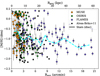 |
Fig. 9. Globular cluster metallicities as a function of galactocentric distance. Different coloured dots indicate metallicities from different instruments. Smaller back dots refer to metallicities from Alves-Brito et al. (2011). In case multiple metallicities are available, preference is given to OSIRIS over MUSE over FLAMES. The cyan dashed line shows the mean metallicity profile. The black line shows the metallicity of the stellar disc. |
Within one effective radius (Reff = 1.7′ = 4.9 kpc, Kormendy & Westpfahl 1989)7, we find a mean GC metallicity of [M/H] ∼ –0.7 dex, which decreases to ∼ − 1 dex above 3′ (∼ 2 Reff) and stays relatively flat out to ∼12′ (∼ 7 Reff). At larger radii (> 12′), the mean metallicity then drops to [M/H] ∼ − 1.3 dex. The stellar metallicity within the disc also shows a gradient towards lower metallicities at larger separations, but overall the stellar metallicity is higher than that of most GCs (e.g. see also Lamers et al. 2017). Nonetheless, there are a few GCs as metal-rich as the galaxy disc.
While we only have a few metallicities from FLAMES available at large separations, the decrease in the mean GC metallicity with radius is expected as also the mean colour of GCs decreases with radius (Kang et al. 2022). On the other hand, the rather flat profile and the presence of metal-rich GCs out to large separations is observed around other massive galaxies (Usher et al. 2012; Pastorello et al. 2014). For example, Villaume et al. (2020) reported a flat mean metallicity profile for GCs around M 87 out to 8 effective radii with a large scatter of metallicity at all radii, similar to our findings.
5.3. GC metallicity distribution
We show the GC metallicities as binned histograms in Fig. 10. In top panels, we show the full sample of GC metallicities in the grey histograms. As described before, we chose OSIRIS metallicities where available over MUSE over FLAMES over the literature sample of Alves-Brito et al. (2011). Based on index-based measurements, Alves-Brito et al. (2011) suggested that the GC metallicity distribution of M 104 is bimodal with peaks at [Fe/H] = −1.44 and −0.66 dex (black histogram in the top left panel). However, we cannot confirm this from our sample as shown in Fig. 10 in the blue histogram in the second panel. Instead, we find a metallicity distribution that is dominated by a broad peak at [M/H] = ∼–1.1 dex and a smaller population of metal-rich GCs. A two-sample Kolmogorov-Smirnov test comparing our sample and that of Alves-Brito et al. (2011) finds a p-value < 0.05, suggesting different distributions, likely because of the different spatial distributions between the samples. Our sample contains many central, metal-rich GCs in the MUSE and OSIRIS samples, which are not as prominent in the sample from Alves-Brito et al. (2011). On the other hand, the FLAMES sample contains many more metal-poor GCs, likely because the FLAMES footprint covers more of the outer GC system.
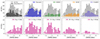 |
Fig. 10. Distribution of GC metallicities. Top row: Full sample of GC metallicities (shown in grey) combining the measurements from Alves-Brito et al. (2011) (black, first panel) and the ones presented here (blue, second panel). Third to fifth panel: GC metallicities from OSIRIS (green), MUSE (orange), and FLAMES (purple). Bottom: GC metallicities in different radial bins. The lines show kernel density estimations scaled to match the counts. The small vertical lines near zero indicate the individual metallicity measurements. |
To explore this in more detail, the bottom panels of Fig. 10 show the GC metallicities in different radial bins, from the centre out to ∼70 kpc (see also Fig. 9). In these histograms, the decreasing mean metallicity becomes evident, as fraction of metal-poor GCs increases with increasing radius. We caution here again that this decrease might also be influenced by a possible saturation of the FLAMES metallicity measurement from the calcium triplet region (Usher et al. 2012). Nevertheless, a decrease in mean metallicity is expected at larger radii due to the increasing fraction of accreted material stemming from metal-poor dwarf galaxies (e.g. Forbes & Remus 2018).
5.4. The formation history of M 104
With their old ages, GCs are often regarded as powerful probes of galaxy evolution. In the traditional picture, metal-poor GCs are thought to originate from accreted low-mass, metal-poor systems. However, since metal-poor GCs can also form in-situ in the host galaxy, either at earlier times or in less enriched regions, assigning individual GCs to either population is a complex problem as simulations suggest (Forbes & Remus 2018; Pfeffer et al. 2023). Likely only GCs with extreme metallicities – either very metal-rich or very metal-poor – can be assigned to either category with confidence.
Comparing the stellar metallicity from the MUSE data (see Fig. 9) shows that M 104 is a metal-rich galaxy, as also found in previous studies (Mould & Spitler 2010). While the MUSE data only probes the inner regions, Cohen et al. (2020) used resolved stellar populations from HST imaging out to almost 40 kpc to study the stellar metallicity. They reported only a negligible fraction of stars below [Z/H] < − 1 dex. Consequently, metal-rich GCs appear to be good tracers of this metal-rich component out to several effective radii, as was also found for other massive galaxies (e.g. Beasley et al. 2008; Peacock et al. 2015; Harris et al. 2016; Fahrion et al. 2020; Villaume et al. 2020). Another indication of this is seen in the different kinematics between the red and blue GCs (Fig. 8), where the red GCs more closely follow the kinematics of the galaxy. Consequently, there are indications that the red GCs are good tracers of the metal-rich spheroid of M 104, which might have been built in-situ of from the accretion of massive, metal-rich satellites. For example, Cohen et al. (2020) proposed that the high metallicity in the far halo of M 104 could be explained by a recent major merger with another massive galaxy (M* ∼ 1011 M⊙). Such a massive galaxy would then also bring in GCs with a broad range of metallicities.
On the other hand, the high velocity dispersion and low rotation at large radii of the blue GCs suggest that at least some of them they were accreted from lower mass systems, building a dynamically hot halo component. The presence of a large range of GC metallicities, including very metal-poor ones, together with an extended number density profile of blue GCs (Kang et al. 2022) implies a rich formation history of M 104 including also minor mergers.
6. Conclusions
In this work, we have presented a new spectroscopic GC catalogue of 499 GCs based on previous works (Dowell et al. 2014; Alves-Brito et al. 2011) and new spectra from OSIRIS, MUSE, and FLAMES. We summarise our main findings as follows:
-
Extracting GC spectra from MUSE integral-field spectroscopy allowed us to probe the inner GC system of M 104. From the MUSE data, we extracted the spectra of 139 GCs, including a few that are located within the disc. In addition, 69 GCs were observed with OSIRIS, yielding high S/N spectra, and 94 GCs have high spectral resolution spectra from FLAMES.
-
Combined with the GC catalogue presented by Dowell et al. (2014), we obtained a GC sample of 499 GCs around M 104. Given that the total number of GCs is estimated at 1600–2000, this spectroscopic GC sample constitutes a significant fraction (∼25–30%) of all GCs of M 104.
-
We find good agreement among the velocity measurements of GCs present in multiple samples. Similarly, when comparing the metallicity measurements, we found excellent agreement between metallicities measured from MUSE and OSIRIS. The metallicities obtained by using full spectrum fitting to the FLAMES calcium triplet region spectra show good agreement with other estimates, highlighting the potential of using those spectra for stellar population studies.
-
We modelled the GC velocities with a simple sinusoidal model, and the model suggests that the velocity dispersion decreases with radius. The rotation amplitude is low, illustrating that the GC system is dispersion-dominated, and it traces the enclosed mass, which is also consistent with previous studies. When separating red and blue GCs, we found that the red GCs have lower dispersions and more closely follow the stellar light, while the blue GCs show rotation only in the very inner region and are more dispersion-dominated. A more detailed discrete dynamical model will be subject of a future project.
-
Based on metallicity measurements of 278 GCs (190 from MUSE, OSIRIS, and FLAMES), we find that the GC system of M 104 shows a large scatter in metallicity, and this scatter persists out to the halo region. Within one effective radius (Reff = 1.7′ = 4.9 kpc), the mean GC metallicity is [M/H] = –0.7 dex, while it decreases to ∼ − 1 dex beyond 3 Reff (15 kpc) and remains at that level out to ∼50 kpc. The metal-rich GCs are as metal-rich as the disc of M 104.
-
We find a complex GC metallicity distribution from the spectroscopic measurements. The total distribution has a broad metal-poor peak at [M/H] = –1 dex and a smaller population of more metal-rich GCs. Exploring the distribution as a function of projected distance shows broad GC metallicity distributions at all radii with a mild trend towards lower metallicities at larger radii, as also seen in the radial metallicity profile. The presence of metal-rich GCs are found at all radii indicates a metal-rich halo, while the broad range of GC metallicities is likely a consequence of the rich formation history of M 104.
Data availability
Full Table D is available at the CDS via https://cdsarc.cds.unistra.fr/viz-bin/cat/J/A+A/702/A59
We note that the effective radius of M 104 has been measured several times using different approaches (e.g. Gadotti & Sánchez-Janssen 2012) with varying results depending on whether the disc and bulge are considered separately. We used the same value as Dowell et al. (2014).
Acknowledgments
We thank the referee for a constructive report that has helped to improve this manuscript. KF acknowledges funding from the European Union’s Horizon 2020 research and innovation programme under the Marie Skłodowska-Curie grant agreement No 101103830. O.M. is grateful to the Swiss National Science Foundation for financial support under the grant number PZ00P2_202104. This work made use of Astropy (http://www.astropy.org): a community-developed core Python package and an ecosystem of tools and resources for astronomy (Astropy Collaboration 2013, 2018, 2022). Based on observations collected at the European Southern Observatory under ESO programmes 60.A-9303 and 114.274W, and at the Gran Telescopio Canarias under programmes GTC24-19A and GTC89-20A. ACS acknowledges support from FAPERGS (grants 23/2551-0001832-2 and 24/2551-0001548-5), CNPq (grants 314301/2021-6, 312940/2025-4, 445231/2024-6, and 404233/2024-4), and CAPES (grant 88887.004427/2024-00).
References
- Alves-Brito, A., Hau, G. K. T., Forbes, D. A., et al. 2011, MNRAS, 417, 1823 [Google Scholar]
- Astropy Collaboration (Robitaille, T. P., et al.) 2013, A&A, 558, A33 [NASA ADS] [CrossRef] [EDP Sciences] [Google Scholar]
- Astropy Collaboration (Price-Whelan, A. M., et al.) 2018, AJ, 156, 123 [Google Scholar]
- Astropy Collaboration (Price-Whelan, A. M., et al.) 2022, ApJ, 935, 167 [NASA ADS] [CrossRef] [Google Scholar]
- Bacon, R., Vernet, J., Borisova, E., et al. 2014, Messenger, 157, 13 [Google Scholar]
- Beasley, M. A. 2020, in Reviews in Frontiers of Modern Astrophysics; From Space Debris to Cosmology (Springer International Publishing: Cham), 245 [Google Scholar]
- Beasley, M. A., Bridges, T., Peng, E., et al. 2008, MNRAS, 386, 1443 [NASA ADS] [CrossRef] [Google Scholar]
- Beasley, M. A., Fahrion, K., Guerra Arencibia, S., Gvozdenko, A., & Montes, M. 2025, A&A, 697, A144 [NASA ADS] [CrossRef] [EDP Sciences] [Google Scholar]
- Bressan, A., Marigo, P., Girardi, L., et al. 2012, MNRAS, 427, 127 [NASA ADS] [CrossRef] [Google Scholar]
- Bridges, T. J., & Hanes, D. A. 1992, AJ, 103, 800 [Google Scholar]
- Bridges, T. J., Ashman, K. M., Zepf, S. E., et al. 1997, MNRAS, 284, 376 [Google Scholar]
- Bridges, T. J., Rhode, K. L., Zepf, S. E., & Freeman, K. C. 2007, ApJ, 658, 980 [Google Scholar]
- Cappellari, M. 2017, MNRAS, 466, 798 [Google Scholar]
- Cappellari, M. 2023, MNRAS, 526, 3273 [NASA ADS] [CrossRef] [Google Scholar]
- Cappellari, M., & Copin, Y. 2003, MNRAS, 342, 345 [Google Scholar]
- Cappellari, M., & Emsellem, E. 2004, PASP, 116, 138 [Google Scholar]
- Cepa, J. 1998, Ap&SS, 263, 369 [Google Scholar]
- Chaturvedi, A., Hilker, M., Cantiello, M., et al. 2022, A&A, 657, A93 [NASA ADS] [CrossRef] [EDP Sciences] [Google Scholar]
- Chen, Y., Bressan, A., Girardi, L., et al. 2015, MNRAS, 452, 1068 [Google Scholar]
- Chung, C., Yoon, S.-J., Lee, S.-Y., & Lee, Y.-W. 2016, ApJ, 818, 201 [NASA ADS] [CrossRef] [Google Scholar]
- Coelho, P. R. T. 2014, MNRAS, 440, 1027 [Google Scholar]
- Cohen, R. E., Goudfrooij, P., Correnti, M., et al. 2020, ApJ, 890, 52 [NASA ADS] [CrossRef] [Google Scholar]
- Crosby, E., Jerjen, H., Müller, O., et al. 2024, MNRAS, 527, 9118 [Google Scholar]
- Crosby, E., Mateo, M., Escala, I., et al. 2025, MNRAS, 536, 2072 [Google Scholar]
- Czesla, S., Schröter, S., Schneider, C. P., et al. 2019, Astrophysics Source Code Library [record ascl:1906.010] [Google Scholar]
- Dowell, J. L., Rhode, K. L., Bridges, T. J., et al. 2014, AJ, 147, 150 [Google Scholar]
- Emsellem, E. 1995, A&A, 303, 673 [NASA ADS] [Google Scholar]
- Errani, R., Peñarrubia, J., & Walker, M. G. 2018, MNRAS, 481, 5073 [CrossRef] [Google Scholar]
- Evans, N. W., Wilkinson, M. I., Perrett, K. M., & Bridges, T. J. 2003, ApJ, 583, 752 [NASA ADS] [CrossRef] [Google Scholar]
- Fahrion, K., Lyubenova, M., van de Ven, G., et al. 2019, A&A, 628, A92 [NASA ADS] [CrossRef] [EDP Sciences] [Google Scholar]
- Fahrion, K., Lyubenova, M., Hilker, M., et al. 2020, A&A, 637, A26 [NASA ADS] [CrossRef] [EDP Sciences] [Google Scholar]
- Fahrion, K., Beasley, M. A., Gvozdenko, A., et al. 2025, A&A, 697, A145 [NASA ADS] [CrossRef] [EDP Sciences] [Google Scholar]
- Forbes, D. A., & Remus, R.-S. 2018, MNRAS, 479, 4760 [Google Scholar]
- Forbes, D. A., Grillmair, C. J., & Smith, R. C. 1997, AJ, 113, 1648 [Google Scholar]
- Forbes, D. A., Alabi, A., Brodie, J. P., et al. 2017, AJ, 153, 114 [Google Scholar]
- Forbes, D. A., Read, J. I., Gieles, M., & Collins, M. L. M. 2018, MNRAS, 481, 5592 [NASA ADS] [CrossRef] [Google Scholar]
- Foreman-Mackey, D., Hogg, D. W., Lang, D., & Goodman, J. 2013, PASP, 125, 306 [Google Scholar]
- Gadotti, D. A., & Sánchez-Janssen, R. 2012, MNRAS, 423, 877 [NASA ADS] [CrossRef] [Google Scholar]
- Grasser, N., Arnaboldi, M., Barbosa, C. E., et al. 2024, A&A, 683, A8 [NASA ADS] [CrossRef] [EDP Sciences] [Google Scholar]
- Guérou, A., Krajnović, D., Epinat, B., et al. 2017, A&A, 608, A5 [Google Scholar]
- Harris, W. E. 2010, arXiv e-prints [arXiv:1012.3224] [Google Scholar]
- Harris, W. E., Harris, H. C., & Harris, G. L. H. 1984, AJ, 89, 216 [Google Scholar]
- Harris, W. E., Spitler, L. R., Forbes, D. A., & Bailin, J. 2010, MNRAS, 401, 1965 [Google Scholar]
- Harris, W. E., Harris, G. L. H., & Alessi, M. 2013, ApJ, 772, 82 [Google Scholar]
- Harris, W. E., Blakeslee, J. P., Whitmore, B. C., et al. 2016, ApJ, 817, 58 [NASA ADS] [CrossRef] [Google Scholar]
- Harris, W. E., Blakeslee, J. P., & Harris, G. L. H. 2017, ApJ, 836, 67 [Google Scholar]
- Hau, G. K. T., Spitler, L. R., Forbes, D. A., et al. 2009, MNRAS, 394, L97 [NASA ADS] [Google Scholar]
- Horne, K. 1986, PASP, 98, 609 [Google Scholar]
- Husser, T. O., Wende-von Berg, S., Dreizler, S., et al. 2013, A&A, 553, A6 [NASA ADS] [CrossRef] [EDP Sciences] [Google Scholar]
- Jardel, J. R., Gebhardt, K., Shen, J., et al. 2011, ApJ, 739, 21 [NASA ADS] [CrossRef] [Google Scholar]
- Jordán, A., McLaughlin, D. E., Côté, P., et al. 2007, ApJS, 171, 101 [CrossRef] [Google Scholar]
- Kang, J., Lee, M. G., Jang, I. S., et al. 2022, ApJ, 939, 74 [Google Scholar]
- Karachentsev, I. D., Makarova, L. N., Brent Tully, R., et al. 2020, A&A, 643, A124 [NASA ADS] [CrossRef] [EDP Sciences] [Google Scholar]
- Kormendy, J., & Westpfahl, D. J. 1989, ApJ, 338, 752 [Google Scholar]
- Kroupa, P. 2001, MNRAS, 322, 231 [NASA ADS] [CrossRef] [Google Scholar]
- Lamers, H. J. G. L. M., Kruijssen, J. M. D., Bastian, N., et al. 2017, A&A, 606, A85 [NASA ADS] [CrossRef] [EDP Sciences] [Google Scholar]
- Larsen, S. S., Forbes, D. A., & Brodie, J. P. 2001, MNRAS, 327, 1116 [Google Scholar]
- Larsen, S. S., Brodie, J. P., Beasley, M. A., & Forbes, D. A. 2002, AJ, 124, 828 [NASA ADS] [CrossRef] [Google Scholar]
- Le, M. N., & Cooper, A. P. 2025, ApJ, 978, 33 [Google Scholar]
- Lim, S., Peng, E. W., Côté, P., et al. 2025, ApJS, 276, 34 [Google Scholar]
- Marigo, P., Bressan, A., Nanni, A., Girardi, L., & Pumo, M. L. 2013, MNRAS, 434, 488 [Google Scholar]
- Martínez-Delgado, D., Román, J., Erkal, D., et al. 2021, MNRAS, 506, 5030 [CrossRef] [Google Scholar]
- McQuinn, K. B. W., Skillman, E. D., Dolphin, A. E., Berg, D., & Kennicutt, R. 2016, AJ, 152, 144 [Google Scholar]
- Mould, J., & Spitler, L. 2010, ApJ, 722, 721 [Google Scholar]
- Pasquini, L., Avila, G., Blecha, A., et al. 2002, Messenger, 110, 1 [NASA ADS] [Google Scholar]
- Pastorello, N., Forbes, D. A., Foster, C., et al. 2014, MNRAS, 442, 1003 [Google Scholar]
- Peacock, M. B., Strader, J., Romanowsky, A. J., & Brodie, J. P. 2015, ApJ, 800, 13 [Google Scholar]
- Pfeffer, J., Kruijssen, J. M. D., Bastian, N., Crain, R. A., & Trujillo-Gomez, S. 2023, MNRAS, 519, 5384 [Google Scholar]
- Pietrinferni, A., Cassisi, S., Salaris, M., & Castelli, F. 2004, ApJ, 612, 168 [Google Scholar]
- Pietrinferni, A., Cassisi, S., Salaris, M., & Castelli, F. 2006, ApJ, 642, 797 [Google Scholar]
- Pota, V., Forbes, D. A., Romanowsky, A. J., et al. 2013, MNRAS, 428, 389 [NASA ADS] [CrossRef] [Google Scholar]
- Prochaska, J., Hennawi, J., Westfall, K., et al. 2020a, J. Open Source Softw., 5, 2308 [NASA ADS] [CrossRef] [Google Scholar]
- Prochaska, J. X., Hennawi, J., Cooke, R., et al. 2020b, https://doi.org/10.5281/zenodo.3743493 [Google Scholar]
- Rhode, K. L., & Zepf, S. E. 2004, AJ, 127, 302 [Google Scholar]
- Sakari, C. M., & Wallerstein, G. 2016, MNRAS, 456, 831 [Google Scholar]
- Schuberth, Y., Richtler, T., Hilker, M., et al. 2010, A&A, 513, A52 [NASA ADS] [CrossRef] [EDP Sciences] [Google Scholar]
- Schuberth, Y., Richtler, T., Hilker, M., et al. 2012, A&A, 544, A115 [NASA ADS] [CrossRef] [EDP Sciences] [Google Scholar]
- Spitler, L. R., Larsen, S. S., Strader, J., et al. 2006, AJ, 132, 1593 [Google Scholar]
- Sutter, J., & Fadda, D. 2022, ApJ, 941, 47 [NASA ADS] [CrossRef] [Google Scholar]
- Usher, C., Forbes, D. A., Brodie, J. P., et al. 2012, MNRAS, 426, 1475 [Google Scholar]
- Usher, C., Forbes, D. A., Brodie, J. P., et al. 2015, MNRAS, 446, 369 [NASA ADS] [CrossRef] [Google Scholar]
- Vazdekis, A., Casuso, E., Peletier, R. F., & Beckman, J. E. 1996, ApJS, 106, 307 [Google Scholar]
- Vazdekis, A., Sánchez-Blázquez, P., Falcón-Barroso, J., et al. 2010, MNRAS, 404, 1639 [NASA ADS] [Google Scholar]
- Vazdekis, A., Koleva, M., Ricciardelli, E., Röck, B., & Falcón-Barroso, J. 2016, MNRAS, 463, 3409 [Google Scholar]
- Verro, K., Trager, S. C., Peletier, R. F., et al. 2022, A&A, 661, A50 [NASA ADS] [CrossRef] [EDP Sciences] [Google Scholar]
- Villaume, A., Foreman-Mackey, D., Romanowsky, A. J., Brodie, J., & Strader, J. 2020, ApJ, 900, 95 [Google Scholar]
- Wakamatsu, K. I. 1977, PASP, 89, 267 [Google Scholar]
- Weilbacher, P. M., Palsa, R., Streicher, O., et al. 2020, A&A, 641, A28 [NASA ADS] [CrossRef] [EDP Sciences] [Google Scholar]
Appendix A: Completeness of MUSE data
While multi-object spectroscopy has long been used to derive spectroscopic GC catalogues around galaxies, using MUSE integral field spectroscopy to probe the more central regions is a more recent approach (e.g. Fahrion et al. 2019, 2020; Grasser et al. 2024). To illustrate the capabilities this approach offers in obtaining high quality spectra even in the crowded and bright inner regions of massive galaxies, we briefly explore here the completeness of the MUSE data.
To check how well our approach performed in extracting GC spectra from MUSE data, we compared the V-band magnitudes of MUSE GCs with HST match with all GCs located in the MUSE field of view from the HST catalogues in the top panel of Fig. A.1. As the two histograms show, we can recover all of the GCs brighter than V < 21 mag from the MUSE data. As a measure of completeness, we show also the fraction of GCs in MUSE over all GCs listed in the HST catalogue (a measure of the completeness). Based on this, we find a completeness of 50% at V ≈ 21.5 mag.
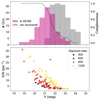 |
Fig. A.1. Completeness and signal-to-noise of the GCs recovered in the MUSE data. Top: Histogram showing the V-band magnitudes of the GCs in MUSE (pink) that have been cross-matched with the HST ACS catalogue (Spitler et al. 2006; Harris et al. 2010). GCs listed in the HST catalogue that were not recovered in MUSE are shown in the grey histogram. The black dashed line shows the fraction of recovered over all HST ACS GCs as a measure of completeness (right y-axis). Bottom: Signal-to-noise ratio of the MUSE GCs as a function of V-band magnitude. The total exposure time of the corresponding MUSE pointing is shown by the colour. |
In the bottom panel of Fig. A.1, we show the S/N of the MUSE GCs as a function of their V-band magnitude. The points are colour-coded by the total exposure time of the MUSE pointing position in which the GCs are located, showing that the GCs in the fields with larger exposure times consistently have higher S/N values, as expected. However, there is considerable scatter, likely due to the varying galaxy background brightness. Consequently, also the completeness shown in the top panel is a complex function of intrinsic GC brightness, exposure time, and galaxy background brightness.
Appendix B: Velocity and metallicity distributions in the central region
As an addition to Fig. 5, Fig. B.1 shows the spatial distributions of velocities and metallicities in the central 5′× 5′.
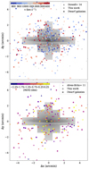 |
Fig. B.1. Spatial distribution of GC velocities (left) and metallicities (right), in the central 5′× 5′. The MUSE white light image is shown in grey. Circles refer to this work, triangles refer to GCs listed in the Dowell et al. 2014 and Alves-Brito et al. 2011. The black cross marks the position of SUCD1 (Hau et al. 2009). |
Appendix C: Iron versus total metallicities
As described in Sect. 3.1, we used both the E-MILES and the XSL SSPs to fit the spectra from MUSE, OSIRIS, and FLAMES for testing purposes. In Fig. C.1, we show a comparison between the derived total metallicities from the E-MILES models and the iron metallicities from the XSL SSPs. As this figure shows, the two models agree very well, especially when considering the uncertainties. Only for high metallicities did we observe deviations, and those are likely caused by the differences in the given metallicity grids.
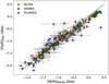 |
Fig. C.1. Total metallicities from fitting the spectra with E-MILES SSPs versus iron metallicities from the XSL SSPs. The different colours show GCs from OSIRIS, MUSE, and FLAMES. The dashed line is the one-to-one relation. |
Appendix D: An updated catalogue of spectroscopically confirmed GCs around M 104
Building on the extensive collection reported in Dowell et al. (2014), we provide here an updated spectroscopic catalogue of GCs around M 104 available combining literature GCs with our measurements from MUSE, FLAMES, and OSIRIS. Table D.1 shows an excerpt of the full catalogue that will be available in machine-readable form on CDS. For illustration purposes, we show here a handful of GCs that are at least in two of our three samples.
Here we briefly review the references that have contributed to this catalogue. As described before, we based our catalogue on the one presented in Dowell et al. (2014). In their work, they presented spectroscopy for 152 unique objects based on spectra from the AAOmega spectrograph on the Anglo-Australian Telescope (AAT) and the Hydra spectrograph at the WIYN telescope at Kitt Peak National Observatory. The remaining sample stems from various sources including 46 velocity measurements from Bridges et al. (1997) based on spectra from the Low Dispersion Survey Spectrograph at the William Herschel Telescope, 16 from Larsen et al. (2002) using Keck Low Resolution Imaging Spectrometer observations, 170 from Bridges et al. (2007) based on data from the Two-Degree Field (2dF) spectrograph at the ATT and WIYN/Hydra data, and 259 from Alves-Brito et al. (2011) that are based on data from the DEep Imaging Multi-Object Spectrograph (DEIMOS) data on Keck. Removing duplicates, the final catalogue of Dowell et al. (2014) lists 579 unique objects. Based on their contamination analysis, they estimated that about 360 of those are genuine GCs of M 104.
In addition to velocities and associated uncertainties, the Dowell et al. (2014) catalogue also lists photometric measurements in V as well as B − V and B − R colours from Rhode & Zepf (2004) based on B, V, and R imaging with Mosaic detector on the Kitt Peak 4m telescope. We adopt those photometric measurements, but combined them with the HST ACS B, V, and R photometry described in Spitler et al. (2006) and Harris et al. (2010) where available. Additionally, we matched our catalogue to the photometric catalogue from Kang et al. (2022) that provides u, g, and i-band magnitudes obtained with MegaCam at the Canada-France-Hawaii Telescope.
Globular cluster catalogue. The full version is available at the CDS.
All Tables
All Figures
|
Fig. 1. Footprints of the different datasets on a greyscale DSS2 image of M 104. MUSE pointings are shown in cyan squares, each with a field of view of 1′×1′. The red circles indicate the field of view of the FLAMES GIRAFFE instrument, with a diameter of 25′, and the orange rectangles show the field of view of OSIRIS, which spans 7.5′×6′. The full greyscale image is 40′ × 40′ (110 kpc × 110 kpc). |
| In the text | |
|
Fig. 2. Spectra of GC #276 for which spectra from MUSE (top), OSIRIS (middle), and FLAMES (bottom) are available. The black lines show the data, and the blue and red lines are the fits with PPXF. Shaded regions were excluded due to sky line residuals. The MUSE and OSIRIS spectra were fitted with XSL SSPs, while we used high resolution stellar models from Coelho (2014) to fit the FLAMES spectrum shown here. |
| In the text | |
|
Fig. 3. Distribution of GCs extracted from MUSE data. Individual GCs are marked with dots colour-coded according to their LOS velocity. Small dots are GC candidates without match to the HST catalogue from Spitler et al. (2006) and Harris et al. (2010). The greyscale image shows the white light image from MUSE. |
| In the text | |
|
Fig. 4. Outlier removal based on GC velocities and projected distances. Top: Line-of-sight velocities as a function of projected galactocentric distance for the full sample of 721 unique sources. Different colours refer to different samples. In case a source is found in multiple samples, only the velocity with the smallest uncertainty is shown. Bottom: Difference between mN and mN − 1 as a function of GC number N (left, see Eq. (1)) and the derivative (right). The vertical grey line indicates our chosen cut-off Ncut = 222, right after the last big jump as seen in the derivative. From this value, the corresponding vmax(R) curve was derived, which is shown as the grey dashed line in the top panel. The shaded regions show the curves when assuming Ncut ± 5. |
| In the text | |
|
Fig. 5. Spatial distribution of GC velocities (top) and metallicities (bottom). The large panels on the left show the full distribution of velocities and metallicities, respectively. Circles refer to this work; triangles refer to GCs listed in the Dowell et al. (2014) and Alves-Brito et al. (2011). Black crosses show dwarf galaxy candidates near M 104 from Crosby et al. (2024). The smaller panels on the right side show the velocities and metallicities in different bins, as indicated in the panel titles. Fig. B.1 shows a zoom-in of the central 5′ × 5′. |
| In the text | |
|
Fig. 6. Comparison of LOS velocities. Black dots are all the GCs found in both samples as indicated by the titles of the panels. Large pink circles are GCs where the velocity uncertainty in both samples is less than 20 km s−1. In the bottom-left corner, we report the p-value of a paired t-test. |
| In the text | |
|
Fig. 7. Comparison of GC metallicities. The first sample reference in the panel title refers to the x-axis and the second to the y-axis. The grey dashed line is the one-to-one relation. We note that the literature metallicities from Alves-Brito et al. (2011) refer to iron metallicities, while we show here the total metallicities inferred from the E-MILES SSP models. |
| In the text | |
|
Fig. 8. Results of the simple kinematic model as a function of radius. Top left: GC system rotation amplitude vrot for all GCs in purple. The black line shows the LOS velocities of the stellar component, taken along a slit 0.4′ above the plane of the disc. Top right: Velocity dispersion of the full GC sample σGCS in purple. Within the rotation-dominated disc, the dispersion is significantly lower than off-plane. Bottom panels: GC rotation amplitude and dispersion for the red and blue GC subpopulations, separately. |
| In the text | |
|
Fig. 9. Globular cluster metallicities as a function of galactocentric distance. Different coloured dots indicate metallicities from different instruments. Smaller back dots refer to metallicities from Alves-Brito et al. (2011). In case multiple metallicities are available, preference is given to OSIRIS over MUSE over FLAMES. The cyan dashed line shows the mean metallicity profile. The black line shows the metallicity of the stellar disc. |
| In the text | |
|
Fig. 10. Distribution of GC metallicities. Top row: Full sample of GC metallicities (shown in grey) combining the measurements from Alves-Brito et al. (2011) (black, first panel) and the ones presented here (blue, second panel). Third to fifth panel: GC metallicities from OSIRIS (green), MUSE (orange), and FLAMES (purple). Bottom: GC metallicities in different radial bins. The lines show kernel density estimations scaled to match the counts. The small vertical lines near zero indicate the individual metallicity measurements. |
| In the text | |
|
Fig. A.1. Completeness and signal-to-noise of the GCs recovered in the MUSE data. Top: Histogram showing the V-band magnitudes of the GCs in MUSE (pink) that have been cross-matched with the HST ACS catalogue (Spitler et al. 2006; Harris et al. 2010). GCs listed in the HST catalogue that were not recovered in MUSE are shown in the grey histogram. The black dashed line shows the fraction of recovered over all HST ACS GCs as a measure of completeness (right y-axis). Bottom: Signal-to-noise ratio of the MUSE GCs as a function of V-band magnitude. The total exposure time of the corresponding MUSE pointing is shown by the colour. |
| In the text | |
|
Fig. B.1. Spatial distribution of GC velocities (left) and metallicities (right), in the central 5′× 5′. The MUSE white light image is shown in grey. Circles refer to this work, triangles refer to GCs listed in the Dowell et al. 2014 and Alves-Brito et al. 2011. The black cross marks the position of SUCD1 (Hau et al. 2009). |
| In the text | |
|
Fig. C.1. Total metallicities from fitting the spectra with E-MILES SSPs versus iron metallicities from the XSL SSPs. The different colours show GCs from OSIRIS, MUSE, and FLAMES. The dashed line is the one-to-one relation. |
| In the text | |
Current usage metrics show cumulative count of Article Views (full-text article views including HTML views, PDF and ePub downloads, according to the available data) and Abstracts Views on Vision4Press platform.
Data correspond to usage on the plateform after 2015. The current usage metrics is available 48-96 hours after online publication and is updated daily on week days.
Initial download of the metrics may take a while.