© The Authors 2025

1 Introduction

Interstellar ices are a key component of the coldest and densest phases of the interstellar medium, profoundly influencing both the physical and chemical evolution of molecular clouds and the processes of star and planet formation (Boogert et al. 2015). One of the most prominent tracers of these ices is the broad 3 μm absorption feature, which arises primarily from the O–H stretching mode in solid H₂O, but whose profile is shaped by additional constituents such as CH₃OH and NH₃·H₂O and by the physical structure of icy grain mantles (e.g., Tielens et al. 1984; Baratta & Strazzulla 1990; Boogert et al. 2011; Noble et al. 2013; McClure et al. 2023). This feature not only signals the presence of water ice but also encodes information about the composition, environment, and evolutionary history of dust grains in molecular clouds.

Over the past decades, tremendous observational and theoretical efforts have been devoted to unraveling the complexity of interstellar ices and their composition (see, e.g., Hudgins et al. 1993; Boogert et al. 2015; Dartois et al. 2024, and references therein). Laboratory experiments and astrochemical modeling have revealed that interstellar ices are not simple, pure substances but rather complex mixtures whose spectral features are sensitive to temperature, composition, and grain morphology (Hudgins et al. 1993; Baratta & Strazzulla 1990; Smith et al. 1993). Observationally, the 3 μm feature has been a cornerstone for tracing ice in the Galaxy, but its study has been hindered by significant technical challenges. Ground-based observations in this wavelength regime are hampered by strong telluric absorption, requiring exceptionally careful calibration and data reduction (e.g., Danielson et al. 1965; Knacke et al. 1969; Gillett & Forrest 1973; Murakawa et al. 2000; Chiar et al. 2011). Even when high-quality spectra can be obtained, deriving accurate optical depths for the 3 μm feature is complicated by uncertainties in the underlying dust extinction law, the spectral type of the background star, and the presence of overlapping features from other species (e.g., Boogert et al. 2011, 2013; Madden et al. 2022).

The advent of space-based observatories has dramatically advanced the field. The Spitzer Space Telescope (Werner et al. 2004; Fazio et al. 2004), with its Infrared Spectrograph (IRS; Houck et al. 2004), has enabled systematic studies of ice absorption features in a wide range of environments, providing a wealth of high-quality spectra that have shaped our current understanding of ice chemistry and distribution (e.g., Boogert et al. 2011, 2013; Madden et al. 2022). More recently, the James Webb Space Telescope (JWST; Gardner et al. 2006; Greene et al. 2017; Jakobsen et al. 2022) has begun to deliver unprecedented sensitivity and spectral resolution in the mid-infrared, revealing new details in the structure and composition of interstellar ices and enabling studies of even fainter and more embedded sources (McClure et al. 2023; Dartois et al. 2024; Rocha et al. 2025; Smith et al. 2025).

Looking ahead, the Spectro-Photometer for the History of the Universe, Epoch of Reionization, and Ices Explorer mission (SPHEREx; Crill et al. 2020) will provide the first all-sky near-infrared spectral survey, systematically mapping ice absorption features such as H₂O, CO, and CO₂. This promises a statistical revolution in our understanding of the Galactic ice reservoir and its environmental dependence.

Despite these advances, most current approaches to ice mapping rely on spectroscopic data for individual sources, which can be observationally expensive and limited in spatial coverage or depth. In this manuscript, in anticipation of results from SPHEREx, I present a new approach: a parameterization of the peak optical depth of the 3 μm ice absorption feature (hereinafter referred to as ${\tau }_{3.0}^{max}$) based on broadband infrared photometry. By leveraging photometric data archives from surveys such as the Wide-Field Infrared Survey Explorer (WISE; Wright et al. 2010) and Spitzer and by calibrating the method with a carefully constructed literature sample, I demonstrate that it is possible to robustly and efficiently trace interstellar ices on Galactic scales.

2 The ice color excess

The presence of water ice and other frozen constituents on dust grains introduces absorption features into the infrared spectra of background stars. Quantifying the additional extinction caused by these icy grains – beyond common dust extinction – is essential for tracing the distribution and abundance of interstellar ices. In this section, I introduce the concept of the ice color excess method ICE, review its physical basis and observational motivation, and present two definitions used to isolate and measure the contribution of ices to the observed extinction.

2.1 Physical background and motivation

The O–H stretch in H₂O and CH₃OH, as well as the N–H stretch in the NH₃·H₂O hydrate, produce a broad absorption band approximately 1 μm wide, peaking at around 3 μm. Consequently, and similar to dust extinction, this additional absorption component significantly affects photometric measurements at these wavelengths.

Figure 1 presents a selection of infrared passbands (see Sect. 5 for further details) and spectral energy distributions (SEDs) for three distinct stellar sources. The upper panel displays the transmission curves of widely used passbands¹, ordered by increasing effective wavelength: K_S, W₁, I₁, L′, I₂, and W₂. The K_S passband (Persson et al. 1998) is widely used in ground-based surveys such as the Two Micron All Sky Survey (2MASS; Skrutskie et al. 2006), while the L′ filter (e.g., Simons & Tokunaga 2002) is also employed in ground-based observations, though it is less commonly available. The W₁ and W₂ passbands were used by the Wide-field Infrared Survey Explorer (WISE; Wright et al. 2010), and I₁ and I₂ by the Spitzer Space Telescope.

Specifically, three passbands cover (parts of) the broad absorption profile: W₁ covers wavelengths from approximately 2.75 to 3.87 μm, with an effective wavelength of 3.35 μm. Similarly, the I₁ passband covers wavelengths from 3.13 μm–3.96 μm, with an effective wavelength of 3.51 μm. The L′ passband, as for example used in the (now decommissioned) VLT NACO instrument, ranges from approximately 3.4 to 4.3 μm and has an effective wavelength of 3.8 μm.

The lower panel of Fig. 1 shows SEDs – specifically the flux density as a function of wavelength – for three stellar sources, each rescaled for visualization. The spectrum of NIR38, a star in the background of the Chamaeleon I molecular cloud observed with JWST (McClure et al. 2023), is shown in red, rescaled to a median flux density of 1 mJy between 4.8 and 5.2 μm. The black line represents the spectrum of Vega from the STScI CALSPEC database (Bohlin et al. 2014), rescaled in the same way as NIR38. The light blue line shows the spectrum of source 15 (see Table A.2), obtained with the X-shooter instrument (Vernet et al. 2011) under ESO program ID 090.C-0050(A), and rescaled to match Vega between 2.0 and 2.4 μm. Among all sources in the final selection (see Sect. 5.2), this was the only one with a NIR spectrum available in the ESO Science Portal².

Given the broad 3 μm absorption feature, it is evident that photometric measurements of sources in the background of ice-rich dust clouds are strongly affected by its presence. In particular, the W₁ and I₁ passbands coincide with the deepest parts of the absorption feature. However, only the W₁ filter fully covers the peak of the optical depth spectrum located at about 3.0 μm. The W₂ and I₂ passbands are influenced by absorption from icy grain constituents such as ¹²CO₂ and ¹²CO (e.g., McClure et al. 2023). In contrast, the K_S passband remains unaffected by ice-related extinction, making it a robust tracer for extinction caused by dust grains at these wavelengths, independent of the presence of ices.

Given the characteristics of these passbands, Fig. 1 demonstrates that photometric measurements with filters covering the broad 3 μm ice absorption profile are significantly affected by an ice extinction component in addition to dust attenuation. Consequently, the ice extinction component – superimposed on dust extinction – can theoretically be measured in a manner analogous to established dust extinction techniques.

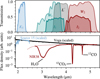Fig. 1 Infrared passbands and SEDs. The upper panel illustrates transmission curves for the infrared passbands KS, W1, I1, L′, I2, and W2. The lower panel presents the SEDs of three distinct sources: the light blue line represents an X-shooter spectrum of source 15 (refer to Table A.2), the solid red line corresponds to the source NIR38, and the black line depicts Vega. All spectra have been rescaled to facilitate a better comparison.

2.2 Color excess approach

Arguably, the most popular method to map dust extinction in the Galaxy is the Near-Infrared Color Excess (NICE) method (Lada et al. 1994). This method, along with its successors NICER (Lombardi & Alves 2001), PNICER (Meingast et al. 2017), and XNICER (Lombardi 2018), relates the measured photometric color excess of stars to the column density of (molecular) hydrogen. In general, the color excess is defined as $$E(m_1-m_2)=(m_1-m_2)-{(m_1-m_2)}_0=A_{m_1}-A_{m_2},$$(1)

where m₁ and m₂ refer to flux measurements in magnitudes in two passbands, (m₁ − m₂)₀ denotes the intrinsic color of a source and A_m1 and A_m2 refer to the amount of extinction in these passbands also in magnitudes. Since their inception and through subsequent advancements, the methods to determine dust extinction have proven to be robust estimators of density information in the interstellar medium (e.g., Goodman et al. 2009; Lombardi et al. 2014; Meingast et al. 2018; Zhang & Kainulainen 2022).

In the context of extinction by icy grains, this concept can be extended further. Given an observed color $$(m_1-m_2)={(m_1-m_2)}_0+E(m_1-m_2),$$(2)

the color excess can be decomposed into distinct dust and ice components: $$(m_1-m_2)={(m_1-m_2)}_0+E{(m_1-m_2)}_{\mathrm{d}\mathrm{u}\mathrm{s}\mathrm{t}}+E{(m_1-m_2)}_{\mathrm{i}\mathrm{c}\mathrm{e}}.$$(3)

This equation defines the principal observable of the ICE method: $$\mathrm{\Lambda }(m_1-m_2)\equiv E{(m_1-m_2)}_{\mathrm{i}\mathrm{c}\mathrm{e}}$$(4) $$=(m_1-m_2)-{(m_1-m_2)}_0-E{(m_1-m_2)}_{\text{dust\hspace{0.17em}}}.$$(5)

This formulation shows that the color excess due to ices can be measured if both the intrinsic color of the star and the extinction caused by dust along the line of sight can be independently determined.

However, both dust and ice extinction are encoded in the single observed color value. Therefore, it becomes necessary to estimate the dust extinction using passbands that are not affected by absorption arising from the presence of ices. Given the well-established dust extinction techniques at near-infrared wavelengths and the absence of significant ice absorption features in the K_S passband (see Fig. 1), E(m₁ − m₂)_dust at wavelengths affected by ice can be estimated by extrapolating the extinction law. A practical implementation for measuring Λ is given by $$\mathrm{\Lambda }(m_1-m_2)=(m_1-m_2)-{(m_1-m_2)}_0-A_{K_S}\cdot \mathrm{\Psi }(m_1,m_2),$$(6)

where Ψ can be determined from the shape of the extinction law: $$\mathrm{\Psi }(m_1,m_2)=\frac{E{(m_1-m_2)}_{\mathrm{d}\mathrm{u}\mathrm{s}\mathrm{t}}}{A_{K_S}}.$$(7)

The term (m₁ − m₂) can be obtained from photometric measurements, the intrinsic color (m₁ − m₂)₀ must be measured or modeled, A_KS can be computed from passbands unaffected by ice extinction (a practical example is near-infrared JHK_S photometry), and Ψ(m₁, m₂) can be derived from theoretical or empirically deduced extinction curves.

2.3 Reddening-free index approach

The procedure described in the preceding section for measuring the ice color excess requires knowledge of the absolute extinction caused by interstellar dust. Alternatively, it is theoretically possible to define a reddening-free color metric that does not rely on a direct measurement of dust extinction. This concept originates from the work of Johnson & Morgan (1953), who introduced the quantity $$Q=(U-B)-\frac{E(U-B)}{E(B-V)}\cdot (B-V),$$(8)

where Q is constructed to be independent of dust reddening. However, this definition does not account for intrinsic stellar colors.

Expanding on this idea, one can define a dust-reddening-free index, Q′, that also removes the dependence on intrinsic colors: $$Q^{\mathrm{\prime }}\equiv E(m_1-m_2)-\frac{E{(m_1-m_2)}_{\mathrm{d}\mathrm{u}\mathrm{s}\mathrm{t}}}{E{(m_2-m_3)}_{\mathrm{d}\mathrm{u}\mathrm{s}\mathrm{t}}}\cdot E(m_2-m_3),$$(9)

where m₁, m₂, and m₃ are magnitudes in three different passbands.

For notational simplicity, let E(m₁ − m₂) = E₁₂ and recall that E₁₂ = A_m1 − A_m2, with A representing extinction in magnitudes. Equation (9) can then be rearranged as: $$Q^{\mathrm{\prime }}=E_{12,\text{dust}}+E_{12,\text{ice}}-\frac{E_{12,\text{dust}}}{E_{23,\text{dust}}}\cdot (E_{23,\text{dust}}+E_{23,\text{ice}})$$(10) $$=E_{12,\mathrm{d}\mathrm{u}\mathrm{s}\mathrm{t}}-\frac{E_{12,\mathrm{d}\mathrm{u}\mathrm{s}\mathrm{t}}}{E_{23,\mathrm{d}\mathrm{u}\mathrm{s}\mathrm{t}}}\cdot E_{23,\mathrm{d}\mathrm{u}\mathrm{s}\mathrm{t}}+E_{12,\mathrm{i}\mathrm{c}\mathrm{e}}-\frac{E_{12,\mathrm{d}\mathrm{u}\mathrm{s}\mathrm{t}}}{E_{23,\mathrm{d}\mathrm{u}\mathrm{s}\mathrm{t}}}\cdot E_{23,\mathrm{i}\mathrm{c}\mathrm{e}}$$(11) $$=A_{m_1,\text{ice}}-A_{m_2,\text{ice}}-\frac{E_{12,\text{dust}}}{E_{23,\text{dust}}}\cdot (A_{m_2,\text{ice}}-A_{m_3,\text{ice}}).$$(12)

In the optimal case – where the passbands m₁ and m₃ do not overlap with any extinction features originating from ices – Eq. (12) reduces to $$Q^{\mathrm{\prime }}=-A_{m_2,\text{\hspace{0.17em}ice\hspace{0.17em}}}\cdot [1+\frac{E{(m_1-m_2)}_{\text{dust\hspace{0.17em}}}}{E{(m_2-m_3)}_{\text{dust\hspace{0.17em}}}}].$$(13)

For a case where passband m₃ also covers the 3 μm feature Eq. (12) becomes $$Q^{\mathrm{\prime }}=A_{m_3,\text{ice}}\cdot \frac{E{(m_1-m_2)}_{\text{dust}}}{E{(m_2-m_3)}_{\text{dust}}}-A_{m_2,\text{ice}}\cdot [1+\frac{E{(m_1-m_2)}_{\text{dust}}}{E{(m_2-m_3)}_{\text{dust}}}],$$(14)

dampening the signal strength.

Similar to the color excess approach, the practical implementation can follow a relatively straightforward approach: Q′ can be determined using Eq. (9), given that intrinsic colors and the dust extinction law are known.

3 Sources of uncertainty

Having outlined the methodology for the ICE method in Sects. 2.2 and 2.3 with two separate approaches, it is essential to consider the various sources of error that affect measurements in practice. Random errors are primarily associated with the precision of stellar flux measurements. In this regard, advances in instrumentation and the advent of large-scale surveys and homogeneous data processing techniques have reduced these uncertainties to the millimagnitude level for millions of sources across the sky. As a result, the dominant sources of uncertainty in measuring the ice color excess are systematic in nature.

The following sections address the most significant systematic error sources: uncertainties in the dust extinction law, intrinsic stellar colors, source variability, and variations in the shape of the 3 μm ice absorption profile.

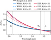Fig. 2 Extinction curves normalized to their value at the effective wavelength of the W1 passband. The different lines correspond to various dust models and R(V) values, as indicated in the legend. WD01 refers to the models of Weingartner & Draine (2001), and D03 to those of Draine (2003). The curves illustrate how both the choice of dust model and R(V) parameter affect the wavelength dependence of extinction.

3.1 Dust extinction law

To accurately determine the color excess attributable to interstellar ices, it is essential to disentangle the extinction caused by ices from that produced by dust. As discussed in Sect. 2, this process requires adopting a dust extinction law that characterizes the relative contributions to extinction across different passbands. However, the precise form of the extinction law is often uncertain and can vary not only between different lines of sight, but also along a single line of sight. To assess the systematic impact of this uncertainty on ice color excess measurements, I compare several commonly used extinction laws, examining how their variations affect the results. The dust extinction laws considered here are those of Weingartner & Draine (2001, WD01), Draine (2003, D03), and Boogert et al. (2011). For both WD01 and D03, I include curves corresponding to R(V) = A_V/E(B − V) values of 3.1, 4.0, and 5.5.

Figure 2 displays these extinction laws over the wavelength range from 1.9 to 3.8 μm, normalized to their values at the effective wavelength of the W₁ passband. The plot demonstrates that the extinction law flattens toward the mid-infrared. This is because, for dust grains much smaller than the wavelength of light, extinction is dominated by absorption. As grains grow to micron-scale sizes, however, scattering becomes increasingly important in the infrared, resulting in a noticeable flattening of the extinction curve at wavelengths greater than about 3 μm (e.g., Dartois et al. 2024). Consequently, the difference between extinction laws in the W₁ and I₁ passbands is much smaller than for pairs involving, for example, the K_S band at about 2.2 μm. For instance – given the set of extinction laws listed above – A_KS/A_W1 ranges from 1.6 to 2.3 – a difference of about 40% between the various curves – whereas A_W1/A_I1 varies by only about 6%, from 1.04 to 1.1.

More specifically, among the extinction laws considered, the factor Ψ(K_S, W₁) – as defined in Eq. (7) – ranges from 0.37 to 0.56, representing a variation of approximately 50%. In contrast, Ψ(W₁, I₁) exhibits a smaller variation of about 30%, ranging from 0.03 to 0.039. These substantial uncertainties highlight the importance of the absolute values of Ψ(m₁, m₂) in the error budget. For a given value of A_KS, the final term in Eq. (6) will have a larger impact on Λ when passbands with greater wavelength separations are used. Similarly, for the dust-reddening-free index Q′ (see Sect. 2.3), the ratio E(m₁ − m₂)/E(m₂ − m₃) can significantly influence the total uncertainty. For the specific case of m₁ = K_S, m₂ = W₁, and m₃ = I₁, the different extinction laws yield absolute values between 13.2 and 16.8 (a difference of roughly 30%), thus contributing notably to the uncertainty in Eq. (9). For m₁ = K_S, m₂ = W₁, and m₃ = L′, the corresponding values range from 5.7 to 7.6 (a difference of about 35%).

This analysis demonstrates that the choice of passband combination plays a crucial role in mitigating these uncertainties: selecting filters with closely spaced wavelengths, such as W₁ and I₁, substantially reduces the impact of extinction law variations on the error budget. Conversely, using passbands that are widely separated in wavelength can lead to much larger systematic uncertainties. Careful selection of filter pairs is therefore essential for robust measurements, particularly when the extinction law is not well constrained. The choice of passbands will be discussed in more detail in Sect. 4.

3.2 Intrinsic colors

Another critical aspect of measuring color excess is the accurate determination of intrinsic stellar colors. Fortunately, the spectral energy distribution of stars is relatively flat at infrared wavelengths, as this part of the spectrum lies in the Rayleigh-Jeans regime. As a result, the intrinsic colors of stars in infrared passbands exhibit a much narrower distribution compared to optical wavelengths. This characteristic is one of the main reasons why dust extinction measurements are particularly effective in the infrared (e.g., Majewski et al. 2011).

Nevertheless, determining intrinsic colors remains a challenge, especially in the context of deep, modern surveys. In particular, contamination from extragalactic sources can complicate the color distribution and must be carefully addressed when developing methods to compute color excess (e.g., Meingast et al. 2017). For extinction mapping based on large samples, a rough estimate of the intrinsic color distribution is often sufficient, as the results are averaged over many sources. However, in this work I aim to parametrize ${\tau }_{3.0}^{max}$ using individual stellar colors. Consequently, it is essential to determine the intrinsic color for each star in the sample with high accuracy, and to quantify how uncertainties in intrinsic colors contribute to the overall error budget.

To assess the impact of intrinsic color uncertainties for known spectral types, I computed intrinsic colors using observed stellar spectra from the IRTF Spectral Library³. Synthetic photometry was performed with the PYPHOT package (Fouesneau 2025) on IRTF spectra spanning spectral types F0 to M9, for both dwarfs and giants. The analysis focused on the color indices most relevant to this study: (K_S − W₁)₀ and (W₁ − I₁)₀. Figure 3 visualizes the results: the top panel shows (K_S − W₁)₀ as a function of spectral type, while the bottom panel displays (W₁ − I₁)₀. Results for dwarfs and giants are indicated by blue and red filled circles, respectively. To mitigate noise and systematic errors in individual spectra, I applied least-squares power-law fits of the form (m₁ − m₂)₀ = a · x^b + c, where x denotes the spectral type sequence from F0 to M9. The figure demonstrates that intrinsic colors remain close to zero for most spectral types, with significant deviations appearing only for late-type stars. This is particularly relevant, as M-type stars are the most numerous in the Galaxy, and late-type giants are often targeted in studies of background stars behind molecular clouds due to their high intrinsic luminosity, which enables detection through large amounts of extinction. I note that the apparent deviation for spectral type M8 for the giant sequence in (K_S − W₁)₀ does not affect the analysis, as this color is not used in subsequent steps. The smoothed intrinsic color values derived from the fits are listed in Table A.1, including values for the (W₁ − L′)₀ color for future reference. I use the values obtained from the power-law fits for each spectral type to determine intrinsic colors for individual stars during the calibration of the method in Sect. 6.

To validate the synthetic photometry on IRTF spectra with observational data, I also extracted spectral type information from Simbad⁴. To minimize the effects of extinction, I queried for all sources with Gaia (specifically data release 3; Gaia Collaboration 2016, 2023) parallaxes greater than 1 mas, while young stellar objects, variable stars, and binaries (as identified in Simbad) were excluded. Moreover, I required a cross-match with the unWISE and SESNA datasets (see Sect. 5.1). Due to these selection criteria, the sample of stars with luminosity class III was too small to yield statistically significant results, and the comparison is therefore restricted to dwarfs (n = 733 for K_S − W₁ and n = 462 for W₁ − I₁). In the same way as described above, I determined power-law fits to colors for these stars as a function of listed spectral type and compared the result to the synthetic photometry. My findings from this experiment are in excellent agreement with those derived from the IRTF spectra: the mean deviation is only 0.02 mag in K_S − W₁ and at the mmag level for W₁ − I₁. Only for very late spectral types (later than approximately M5) does the comparison in W₁ − I₁ reveal a systematic deviation of about 0.05 mag. The comparison for dwarfs between the synthetic photometry from IRTF spectra and the Simbad database is visualized in Fig. A.1.

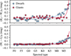Fig. 3 Intrinsic colors for dwarfs (blue symbols) and giants (red symbols) as a function of spectral type, derived from synthetic photometry of IRTF spectra. Solid lines indicate power-law fits to the intrinsic colors for dwarfs (blue) and giants (red), respectively. The upper panel shows intrinsic KS − W1 color, while the lower panel displays W1 − I1. For both color indices, significant deviations from 0 mag are observed only for late spectral types (later than approximately M0).

3.3 Source variability

Another source of systematic uncertainty is the intrinsic variability of stars. In this study, the photometry used to compute color excesses is derived from observations taken at different epochs, sometimes separated by more than a decade. For example, the 2MASS survey collected data between 1997 and 2001, the c2d survey lists I₁ recording dates from 2003 to 2005, and WISE observed from 2009 to 2024 (including NEOWISE; Mainzer et al. 2011). Additionally, some targeted observations of sources to measure the depth of the 3 μm ice feature even predate the 2MASS survey. Since nearly all stars discussed in this paper are giants – stellar types that are often long-period variables with timescales of several years – long-term variability and its potential impact on the results must be carefully considered.

For ensembles of stars, variability is generally less problematic, as the sample mean flux averages out individual stellar fluctuations. However, for individual sources, it is essential to account for variability explicitly. To assess the impact of source variability, I utilize the unTimely source catalog (Meisner et al. 2023), which was constructed by measuring fluxes on a series of unWISE coadds in the W₁ and W₂ passbands, each corresponding to a biannual WISE sky pass. With data spanning from 2010 to 2020, unTimely provides up to 16 measurements per detected source. Given only two data points per year, short-term variations are not well sampled, but the decade-long baseline is well suited to reveal long-term or large-amplitude variability. For the calibration of the method, I use the obtained information on variability from unWISE to construct a quality filter and to add an additional systematic error term in regard to photometric parameters.

3.4 Shape of the absorption profile

Any variation in the shape of the 3 μm ice absorption profile will naturally be reflected in the measured color excess. Several studies have reported that the detailed structure of this absorption feature can vary across different environments (see, e.g., Boogert et al. 2015). In particular, the composition of the ice mixture has a pronounced effect on the red wing of the profile, with species such as NH₃·H₂O and CH₃OH contributing significantly (e.g., Hudgins et al. 1993; Chiar et al. 2011; McClure et al. 2023; Rocha et al. 2025). More recently, Noble et al. (2024) used JWST observations to reveal minor contributions from so-called dangling OH groups on the blue side of the feature, near 2.7 μm.

Despite these variations, there is also evidence that the overall shape of the 3 μm absorption profile toward background stars is relatively stable (Boogert et al. 2011; Madden et al. 2022). To further investigate this, I present in Fig. 4 a comparison of three measured absorption profiles, together with selected laboratory spectra from Hudgins et al. (1993). The red profile corresponds to the star 2MASS J17112005-2727131, a background giant behind the B59 core in the Pipe Nebula. The blue line shows the JWST spectrum for NIR38 (McClure et al. 2023), a background giant behind the Chamaeleon I molecular cloud, while the green line represents Ced 110 IRS4 (2MASS J11064638-7722287; Rocha et al. 2025), a binary protostellar system in Chamaeleon I. Because the optical depth profiles for these sources are not publicly available, I used WebPlotDigitizer⁵ to extract the data from published figures, manually tracing each spectrum and interpolating the results onto a regular wavelength grid with minimal smoothing. Any gaps in the measured spectra were interpolated, and all curves were renormalized to a peak optical depth of 1. For the laboratory data, I selected two mixtures: the dotted black line shows pure water ice (100% H₂O), while the solid black line represents a strong ice mixture (H₂O:CH₃OH:CO:NH₃ = 100:10:1:1), both at a temperature of 10 K.

Figure 4 reveals an apparent similarity among the observed absorption profiles, which also closely match the laboratory spectrum for the strong ice mixture. To quantify how variations in the absorption profile affect the measured color excess, I simulated the impact of each profile on broadband photometry. Specifically, I calculated the fluxes through different passbands as a function of the peak optical depth and derived the resulting color indices. The results are presented in Fig. 5, which shows the standard deviation (solid lines) and maximum difference (dashed lines) in measured colors for all five absorption profiles as a function of optical depth. The black curves correspond to the K_S − W₁ color, while the red curves represent W₁ − I₁.

These simulations demonstrate that the K_S − W₁ color is much more sensitive to variations in the absorption profile than W₁ − I₁. This is because only the W₁ band is affected by ice extinction in the former case, while the K_S band remains unaffected. In contrast, both W₁ and I₁ are affected in the latter, leading to a partial cancellation of profile-dependent effects. Even at large optical depths, the standard deviation in W₁ − I₁ remains at only a few percent. If the pure ice mixture is excluded from this test, the variation in both color indices decreases further: for a peak optical depth of 5, the standard deviation in K_S − W₁ drops to about 10%, and in W₁ − I₁ to approximately 3%.

These findings demonstrate that, depending on the chosen color metric, the ice color excess method can be tuned to either enhance sensitivity to profile shape – potentially enabling the detection of differences in ice composition – or to minimize such sensitivity, thereby providing a robust measurement of ${\tau }_{3.0}^{max}$.

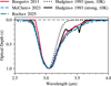Fig. 4 Normalized absorption profiles of the 3 μm feature toward two background stars published by Boogert et al. (2011) and McClure et al. (2023) and one protostar (Rocha et al. 2025) compared with laboratory ice spectra from Hudgins et al. (1993). The observed profiles (red, blue, and green) were extracted from published data and interpolated onto a common wavelength grid. Laboratory spectra correspond to pure water ice (dotted black) and a strong ice mixture (solid black) at 10 K. All profiles are normalized to a peak optical depth of 1 for a direct comparison of the profile shape.

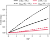Fig. 5 Standard deviation (solid lines) and maximum difference (dashed lines) in KS − W1 (black) and W1 − I1 (red) colors as a function of the peak optical depth of the 3 μm feature, calculated for five absorption profiles (see Fig. 4). The KS − W1 color is significantly more sensitive to variations in the absorption profile, while W1 − I1 remains comparatively stable, enabling robust measurements of ${\tau }_{3.0}^{max}$.

4 Selection of optimal passbands

The selection of suitable photometric passbands is a critical step in reliably measuring ${\tau }_{3.0}^{max}$. The broad 3 μm ice feature, spanning roughly from 2.7 to 3.7 μm, is sampled by a limited set of widely available filters. As shown in Fig. 1, any practical combination for computing the ice color excess will necessarily include W₁, I₁, or, in rare cases, L′. Among these, L′ only covers the red wing of the feature and does not sample the peak of the absorption feature near 3 μm. Moreover, L′ photometry is not broadly available and is typically restricted to small observing programs with specific targets. While such data may still be valuable for probing the red wing of the feature, large-scale studies must rely on the more widely available W₁ and I₁ passbands.

The options for constructing reliable color excess measurements are further constrained by the properties of other available bands. Both W₂ and I₂ are affected by additional ice absorption features and are therefore unsuitable for any color combination described in Sect. 2. The only realistic choices for pairing with W₁ or I₁ are near-infrared passbands such as K_S, which are accessible through large-area surveys like 2MASS, VVV(X), and VISIONS. This leaves three main configurations for calculating the ice color excess: Λ(K_S − W₁), Λ(K_S − I₁), and Λ(W₁ − I₁), as well as their use in the dust-reddening-free index Q′.

The optimal choice of passbands is governed by two main factors: (a) the systematic error budget – dominated by uncertainties in the extinction law – and (b) the availability and quality of the photometric data. Pairing K_S with W₁ offers the advantage of all-sky coverage, but it is limited by the sensitivity of 2MASS and is subject to large systematic uncertainties due to the significant wavelength separation, which amplifies errors related to the extinction law. The same applies to K_S with I₁, with the added limitation that I₁ data do not cover the entire sky. The alternative approach, involving K_S, W₁, and I₁ for Q′, also suffers from large systematic uncertainties for the same reason.

To quantify how the choice of passbands and the underlying uncertainties affect measurements of Λ and Q′, I performed a Monte Carlo simulation that incorporates the various error sources discussed above. For each realization, random errors were assigned to the observed stellar magnitudes (0.01 mag), intrinsic stellar color (0.05 mag), and the measured dust extinction in the K_S passband (0.1 mag). Additionally, one of the seven extinction laws discussed above was randomly selected for each trial. Furthermore, a linear relation between extinction and the peak optical depth of the 3 μm feature was assumed (${\tau }_{3.0}^{max}$ = 0.5A_KS), consistent with literature findings and omitting an explicit ice formation threshold (e.g., Boogert et al. 2011, 2013; Madden et al. 2022). This process was repeated one million times for ${\tau }_{3.0}^{max}$ values ranging from 0 to 5 in steps of 0.05. The results of this experiment are presented in Fig. 6, which displays the standard deviation in the measured ice color excess metrics as a function of ${\tau }_{3.0}^{max}$ for several band combinations. Specifically, the figure shows Λ(K_S − W₁) (solid black line), Λ(W₁ − I₁) (solid red line), Λ(W₁ − L′) (solid blue line), Q′(K_S, W₁, I₁) (gray dashed line), and Q′(K_S, W₁, L′) (dark blue dashed line).

Several key trends emerge from the simulation. Both Q′ metrics exhibit relatively large but almost constant uncertainties across the full range of optical depths. This is because the error budget for Q′ is dominated by uncertainties in the shape of the extinction law or, more specifically, the ratio of color excesses (see Eq. (9)). In contrast, the various definitions of Λ generally yield smaller errors, with the uncertainty increasing nearly linearly with optical depth. The magnitude of this error is strongly dependent on the choice of band combination: Λ(K_S − W₁) shows large uncertainties, reflecting the greater impact of extinction law uncertainties when the wavelength separation between bands is large. Most notably, Λ(W₁ − I₁) and Λ(W₁ − L′) stand out for their remarkably small total error budgets, even at high optical depths. This is a direct consequence of the small wavelength separation between W₁ and I₁ (or L′).

These findings demonstrate that – when considering both the error budget and data availability – the combination of W₁ and I₁ in measuring Λ(W₁ − I₁) provides the most robust and reliable measurement of the ice color excess. The results of the above described simulation highlight that systematic errors remain well controlled for this passband pair, even at high optical depths, due to the small wavelength separation and the resulting reduced sensitivity to extinction law uncertainties. Furthermore, both W₁ and I₁ offer high-precision photometry in key nearby star-forming regions, where future applications of this method are particularly effective thanks to the abundance of background stars and minimal confusion from overlapping clouds along the line of sight. For these reasons, the following analysis focuses on the application of the ICE using the W₁ − I₁ color: $$\mathrm{\Lambda }(W_1-I_1)=(W_1-I_1)-{(W_1-I_1)}_0-A_{K_S}\cdot \mathrm{\Psi }(W_1,I_1).$$(15)

Future studies may extend this approach to other band combinations as our understanding of the dust extinction law improves.

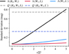Fig. 6 Standard deviation of Λ and Q′ color excess measurements as a function of the peak optical depth of the 3 μm feature, derived from randomly sampling uncertainties in the photometric parameters and the extinction law. Solid lines represent Λ for different band combinations: Λ(KS − W1) in black, Λ(W1 − I1) in red, and Λ(W1 − L′) in blue. Dashed lines show Q′ for the combinations Q′(KS, W1, I1) (gray) and Q′(KS, W1, L′) (dark blue). The simulation demonstrates that Λ(W1 − I1) and Λ(W1 − L′) maintain the lowest total uncertainties, even at high optical depths, due to the small wavelength separation between the bands.

5 Data and observational resources

To calibrate a parametrization for ${\tau }_{3.0}^{max}$ as a function of Λ(W₁ − I₁), I utilize multiple data sources to obtain infrared photometry and spectroscopically measured optical depths. This section provides an overview of the data archives employed and the specific quality criteria used for source selection.

5.1 Infrared photometry

Infrared broadband photometry covering the 3 μm absorption feature is the basis for the computation of the color excess caused by icy grains. In this wavelength range, two major data sources are available, each providing access to millions of individual measurements: data collected by the Spitzer Space Telescope and data from the WISE allsky survey. Both missions provide data for a set of passbands, including the filters W₁ and I₁ that nearly completely cover the broad ice absorption feature at 3 μm (see Fig. 1).

Both WISE and Spitzer provide multiple data releases, including versions tailored to specific sub-surveys conducted by the astronomical community, each of which may itself have several data releases. For WISE, in this manuscript I use the unWISE catalog (Schlafly et al. 2019), which is based on coadds of all publicly available WISE images in the W₁ and W₂ passbands. The unWISE data processing methodology improves the sensitivity limit by approximately 0.7 mag compared to the AllWISE data release (Cutri et al. 2021).

For Spitzer data, several catalogs are accessible via the NASA/IPAC Infrared Science Archive⁶ (IRSA). Among these, the most relevant are those covering prominent, nearby, and actively star-forming molecular clouds, such as Orion, Taurus, Perseus, Ophiuchus, Lupus, Chamaeleon, and Corona Australis. However, data processing methods – and thus data quality – vary across Spitzer products due to the use of diverse pipelines and reduction techniques. To mitigate potential systematic differences, I adopt the Spitzer Extended Solar Neighborhood Archive (SESNA; see Pokhrel et al. 2020 for an overview and a forthcoming publication by Gutermuth et al. for details) as the primary source of Spitzer photometry. SESNA provides a uniformly reduced catalog for several dozen nearby molecular cloud complexes observed during the operational lifetime of Spitzer.

Some regions, however, are not included in SESNA. Notably, the Taurus star-forming complex (Rebull et al. 2010) has not yet been reprocessed in the context of the SESNA project, but catalog data for this region are available through IRSA (Taurus Team 2020). For all remaining lines of sight not covered by SESNA or the Taurus data release, I use data from the Spitzer survey “From Molecular Cores to Planet-Forming Disks” (c2d; Evans et al. 2003).

Near-infrared K_S-band photometry is sourced exclusively from the Two Micron All Sky Survey (Skrutskie et al. 2006). For future applications of the technique presented in this manuscript, more recent wide-field NIR surveys – such as the VISTA Variables in the Via Láctea (VVV; Minniti et al. 2010), its extension VVVX, and especially the VISTA Star Formation Atlas (VISIONS; Meingast et al. 2023) – will be of increasing relevance. The VVV and VVVX surveys cover the Galactic bulge and approximately 150 deg in Galactic longitude along the Milky Way plane. In contrast, VISIONS targets five nearby (d ≲ 500 pc) star-forming regions, providing ideal coverage for future measurements of the ice color excess.

5.2 Optical depth sample

To construct a robust parametrization of ${\tau }_{3.0}^{max}$, I conducted an extensive literature search for spectroscopic measurements of this feature toward stars in the background of molecular clouds. This search identified nine major sources, encompassing a broad range of observing facilities, data quality, and target environments. A summary of the literature sources, telescope facilities, and corresponding symbols used in subsequent plots is provided in Table 1. A detailed overview of the final source list, including adopted spectral types, photometric parameters, extinction, and measured ice color excesses, is given in Table A.2.

Murakawa et al. (2000) used the Wyoming Infrared Observatory (WIRO)⁷ and the Mt. Lemmon Observing Facility (MLFO)⁸ to observe 61 background stars in the Taurus Molecular Cloud. Out of the 61 observed sources, the authors report ${\tau }_{3.0}^{max}$ values for 55 sources, including many cases where the feature was not detected (${\tau }_{3.0}^{max}$ = 0). Boogert et al. (2011) combined Spitzer IRS spectra with ground-based Keck data to observe 33 sources across regions such as Ophiuchus, Serpens, Aquila, and Taurus, thereby sampling a variety of astrophysical environments. For two of these sources, only upper limits of ${\tau }_{3.0}^{max}$ were reported. Chiar et al. (2011) used IRTF and Spitzer/IRS to obtain spectra for ten sources in the IC 5146 (Barnard 168) cloud, with the SpeX instrument (Rayner et al. 2003). Of these, for seven sources ${\tau }_{3.0}^{max}$ was measured. Boogert et al. (2013) presented Spitzer/IRS observations of 32 sources in the Lupus cloud complex. Of these, for 11 sources the ${\tau }_{3.0}^{max}$ measurement corresponds to an upper limit. Noble et al. (2013) provided 30 AKARI (Onaka et al. 2007; Ohyama et al. 2007) spectra, covering regions such as Ophiuchus, Lupus, and Taurus. In this publication, explicit values for ${\tau }_{3.0}^{max}$ were not reported. Hence, I estimated values by eye from the published plots for 13 sources with unambiguous features. Goto et al. (2018) used IRTF/SpeX to observe 21 sources, providing usable ${\tau }_{3.0}^{max}$ values for seven sources in the Pipe Nebula, with the remaining measurements being upper limits. Madden et al. (2022) recorded 49 spectra projected against Perseus and Serpens using Spitzer/IRS and IRTF/SpeX, with 28 ${\tau }_{3.0}^{max}$ measurements in Perseus and 21 in Serpens. In more recent work, McClure et al. (2023) used JWST to observe two highly obscured sources behind the Chamaeleon I cloud, and Smith et al. (2025) expanded this with JWST spectra for 44 background sources in the same region.

For all data sources, I applied a consistent workflow. First, I extracted coordinates, ${\tau }_{3.0}^{max}$ (excluding upper limits), and extinction measurements from the original publications, converting all coordinates to the ICRS reference frame as needed. For the earliest published data from Murakawa et al. (2000), for which coordinates were published in J1950, I visually inspected 2MASS images using Aladin and manually corrected mismatches resulting from imperfect coordinate transformations. For all literature sources reporting individual extinction values in the V passband, these were converted to A_KS using the extinction law of Boogert et al. (2011). Next, I cross-matched the compiled catalogs with the above-listed infrared datasets, including unWISE, c2d, SESNA, and Spitzer Taurus, using a matching radius of 2 arcsec. In all cases, unWISE source coordinates were used as the reference. For Spitzer photometry, I preferred SESNA data, using Taurus and c2d as fallback options in this order.

To ensure high data quality, I imposed a series of strict selection criteria. Foremost, I required an unambiguous cross-match with the unWISE catalog. Additional requirements included an unWISE quality factor on W₁ (qfW1) greater than 0.99, a W₁ magnitude error less than 2 mmag, unWISE Coadd Flags at the central pixel less than or equal to 1, and a W₁ inter-quartile range from unTimely time series below 0.04 mag. For sources with I₁ data from c2d, I required IR1_Q_DET_C = A, IR1_Q_FLUX_M = A, and 10 < IR1_FLUX_C < 100. Moreover, for all sources, the spectral type had to be listed in the corresponding reference.

After cross-matching and applying these quality criteria, the initial set of 282 unique sources was reduced to a final sample of 56 sources suitable for analysis. Notably, none of the JWST measurements could be included, primarily because these sources are too faint to be reliably detected by both Spitzer or WISE. Specifically, for the prominent source NIR 38 first investigated by McClure et al. (2023) both Spitzer and WISE measurements are available, but the source was excluded from subsequent analysis due to significant photometric variability (unWISE peak-to-peak amplitude of 0.31 mag). Conversely, many targets from the earlier publications were removed for being too bright for these satellites. In addition, none of the AKARI measurements from Noble et al. (2013) passed the quality cuts, primarily due to missing quality flags for the flux measurements in the c2d catalog.

Figure 7 shows the positions of the final source selection overlaid on a view of the Milky Way as observed by Planck (Planck Collaboration I 2011) at 857 GHz (350 μm). Different symbols (colors and shapes) represent different literature sources as listed in Table 1. The selected sources span galactic longitudes over more than 180 deg, sampling a wide variety of nearby star-forming regions and providing representative coverage of astrophysical conditions.

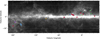Fig. 7 Positions of the final literature sample of background stars with spectroscopically measured 3 μm optical depths, overlaid on a Planck 857 GHz (350 μm) image of the Milky Way. Different symbols (colors and shapes) indicate the data source, as detailed in Table 1. The sample spans more than 180 deg in Galactic longitude, covering a diverse set of nearby star-forming regions.

6 Empirical calibration

With the mathematical framework, the choice of passbands, and the selection of calibration sources from the literature in place, in this section, I present the empirical parametrization for fitting the peak optical depth of the 3 μm ice feature, ${\tau }_{3.0}^{max}$, as a function of the ice color excess Λ(W₁ − I₁). Since the relationship between ${\tau }_{3.0}^{max}$ and any passband combination for Λ is generally non-linear, I adopted a function of the form $${\tau }_{3.0}^{max}=a\cdot \ln (1+b\cdot \mathrm{\Lambda }),$$(16)

with a and b being the free parameters. Furthermore, the form of this equation is physically motivated to pass through the origin: an ice color excess of Λ = 0 must correspond to zero optical depth.

To accurately represent measurement errors in both Λ and ${\tau }_{3.0}^{max}$, several factors are considered. The error on ${\tau }_{3.0}^{max}$ is not always reported in the literature; when missing, I assume a standard deviation of 10% of the value itself. The error budget for Λ is more complex (see Sect. 3). Photometric errors are taken directly from the source catalogs (unWISE, SESNA, Spitzer Taurus, or c2d). For intrinsic colors, I use the smoothed fit from Fig. 3 and adopt a fixed error of 0.02 mag. Errors on extinction (A_KS) are taken from the literature when available, or otherwise set to 0.1 mag. Additionally, I include a systematic error term to account for stellar variability, using the inter-quartile range from unWISE time series photometry, which is typically 0.01 mag. All values for ${\tau }_{3.0}^{max}$ and Λ(W₁ − I₁) used for the fit, and their associated uncertainties are listed in Table A.2 for the final source selection.

The choice of the specific extinction law is a critical aspect of the calibration. Since most high-optical-depth sources in the final sample (${\tau }_{3.0}^{max}$ ≳ 0.5) are from Boogert et al. (2011), I adopt the extinction law published in that work. As discussed in Sect. 3.1, using Λ(W₁ − I₁) minimizes sensitivity to the extinction law, but I emphasize that this calibration is only strictly valid when used with this specific law; caution is required when applying it to other datasets.

To fit the data and account for measurement errors in both variables, I perform the fit using the SciPy curve_fit function, repeating the procedure 100 000 times. In each iteration, I randomly sample all input data (${\tau }_{3.0}^{max}$ and Λ(W₁ − I₁)) from normal distributions defined by the calculated mean value and the propagated uncertainties. This yields a distribution of possible fits and allows for robust estimation of uncertainties in both the a and b parameters in Eq. (16). Given the non-linear parameter space, I report the geometric median as the best-fit solution, i.e., the point minimizing the sum of Euclidean distances to all sampled points. The resulting fit is shown in Fig. 8, where individual data points correspond to literature measurements, the dashed black line shows the best-fit relation, and gray thin solid lines represent 500 random samples from the parameter space. Gray dashed lines mark ${\tau }_{3.0}^{max}$ = 0 and Λ(W₁ − I₁) = 0, the physically meaningful boundaries. The non-linear distribution of a and b values from the sampling is shown in Fig. A.2.

Figure 8 reveals a strikingly tight relation between the peak optical depth ${\tau }_{3.0}^{max}$ and the computed ice color excess Λ(W₁ − I₁) across the entire range of presented optical depths. Only one clear outlier is present, corresponding to a source from Murakawa et al. (2000) (source 14 in Table A.2), which is likely affected by contamination from a nearby bright star. All other measurements fall along a well-constrained relation, resulting in a robust fit. The best-fitting solution is $${\tau }_{3.0}^{max}=-3.51\cdot \ln [1-0.92\cdot \mathrm{\Lambda }(W_1-I_1)].$$(17)

This tight correlation is all the more remarkable given that the data are drawn from a diverse set of sources, each often relying on different telescope facilities, instrumentation, and data processing pipelines, including the methods used to estimate line-of-sight extinction, approaches to continuum fitting, and techniques for measuring ${\tau }_{3.0}^{max}$. The consistency observed here serves as a strong testament to the robustness and general applicability of the ice color excess method.

For error propagation in the derived equation, it is advisable to sample the parameters a and b in logarithmic space, given the non-linearity of the parameter space; specifically, ln(−a) = 1.36 ± 0.5 and ln(−b) = −0.21 ± 0.43. These large 1-σ uncertainties in the logarithmic fit parameters primarily arise from the degeneracy between a and b in the fit function, rather than from scatter in the input data. This degeneracy allows for a broad range of parameter combinations to provide acceptable fits, as illustrated in Fig. A.2. I note that these quoted mean values are intended solely for sampling and do not correspond to the reported best-fit values (i.e., the geometric median).

In Sect. 3.1, I extensively discussed the systematic effect of the shape of the extinction law on the applicability of the method. For reference, I present in Fig. 9 the fits for the relation between ${\tau }_{3.0}^{max}$ and Λ(W₁ − I₁), when different extinction laws are used for the determination of the factor Ψ in Eq. (15). The considered extinction laws are those published by Weingartner & Draine (2001) (blue lines), Draine (2003) (red lines), and Boogert et al. (2011) (black line). The thin black lines correspond to 500 random samples of the fit with the Boogert et al. (2011) extinction law.

The figure demonstrates that even in the case of choosing Λ(W₁ − I₁), which minimizes the impact of the extinction law, significant differences between the fits become visible. However, in the case of using Λ(W₁ − I₁), the presented curves are still within the typical range of uncertainties in the adopted fit of Eq. (17).

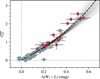Fig. 8 Peak optical depth of the 3 μm ice absorption feature (${\tau }_{3.0}^{max}$) as a function of the ice color excess Λ(W1 − I1) for the calibration sample. The various symbols represent the different literature sources listed in Table 1. Each point represents a literature measurement with propagated uncertainties. The black dashed line shows the best-fit relation, while thin solid lines represent 500 random samples from the fit parameter space. Gray dashed lines mark ${\tau }_{3.0}^{max}$ = 0 and Λ(W1 − I1) = 0.

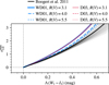Fig. 9 Relation between the peak optical depth of the 3.0 μm ice feature (${\tau }_{3.0}^{max}$) and the ice color excess Λ(W1 − I1) for different assumptions about the extinction law. The fitted curves correspond to extinction laws from Weingartner & Draine (2001) (blue), Draine (2003) (red), and Boogert et al. (2011) (black). While the use of the Λ(W1 − I1) metric minimizes the impact of extinction law uncertainties, systematic differences between the fits remain visible. However, these differences are generally within the typical measurement uncertainties of the calibration. This highlights the importance of adopting a consistent extinction law or recalibrating the method when applying it to different environments.

7 Discussion

The ICE technique presented in this work demonstrates considerable promise for mapping and quantifying the distribution of interstellar ices using widely available infrared broadband photometry. In the formulation presented in this manuscript, the calibration of the method benefits from well-characterized samples where the intrinsic colors of background stars are known – typically through accurate spectral typing. Moreover, for the individual sources, the extinction along the line of sight has been independently determined from spectroscopic measurements. This controlled scenario allows for a robust calibration of the ice color excess and the parameterization of ${\tau }_{3.0}^{max}$. However, scaling this approach to larger and more diverse samples introduces new challenges. In particular, variations in intrinsic stellar colors and uncertainties in extinction estimates become increasingly important when dealing with heterogeneous stellar populations. Future applications will need to address these issues, for example by employing probabilistic methods for stellar classification or leveraging Gaia parallaxes and multi-band photometry to better constrain stellar parameters and extinction.

In particular, the ability to generate spatially resolved ice maps at (sub-)arcminute scales in nearby star-forming regions represents a significant advance over existing techniques, which are often limited by the depth or coverage of spectroscopic surveys. The prospects for applying this technique on a Galactic scale are exceptionally promising. The SESNA catalog alone contains over eight million sources with high-quality infrared photometry, many of which have direct counterparts in the WISE all-sky survey. Even more, the Spitzer program Galactic Legacy Infrared Midplane Survey Extraordinaire (GLIMPSE; Benjamin et al. 2003) contains about 50 million sources, enabling ice mapping in the Galactic Plane. However, similar to dust extinction mapping techniques, multiple overlapping clouds along the line of sight create another challenge to address in constructing ${\tau }_{3.0}^{max}$ maps (Zhang & Kainulainen 2022). Nevertheless, applying the presented method on such scales opens the door to constructing high-resolution, wide-area maps of ${\tau }_{3.0}^{max}$. Such maps would enable detailed studies of the relationship between ice formation, dust properties, and the local interstellar environment.

Moreover, expanding and recalibrating the method to incorporate near-infrared data from 2MASS, VVV(X), and VISIONS increases the number of usable sources by an order of magnitude. In this regard, particularly the 2MASS and unWISE datasets enable an all-sky application of the method. However, a key challenge in extending the ICE method to NIR photometry is the selection of the extinction law, as the conversion from color excess to ${\tau }_{3.0}^{max}$ is highly sensitive to the adopted extinction curve. The extinction law is known to vary significantly, even on relatively small spatial scales (e.g., Green et al. 2025; Zhang & Green 2025), and the ICE method is especially sensitive when combining K_S-band photometry with W₁ data (see Sect. 4). Therefore, it is crucial to employ a standardized approach and, where feasible, recalibrate the method to account for different extinction law characteristics or at least incorporate this systematic effect into the error estimation. The compiled source catalog provided in this work (Table A.2) can act as a valuable resource for such recalibrations, enabling users to tailor the technique to their specific datasets and scientific objectives.

Further, it is instructive to compare the capabilities of this photometric approach with those of JWST, which has rapidly established itself as a premier facility for ice chemistry studies. JWST’s unparalleled sensitivity and spectral resolution in the mid-infrared have revealed exquisite detail in the absorption features of interstellar ices, uncovering subtle compositional variations and previously unknown molecular species (e.g., McClure et al. 2023; Dartois et al. 2024; Rocha et al. 2025). While the ICE method cannot provide the same level of chemical detail or resolve fine spectral structure, it serves as a powerful tool for parameterizing the peak optical depth of the main ice features across large samples and broad spatial scales. In this way, the technique complements the detailed, small-area studies enabled by JWST (Smith et al. 2025), allowing localized chemical findings to be placed into a global Galactic context. Photometric ice maps can be used to investigate ice formation thresholds as reported by, for example, Chiar et al. (2011); Boogert et al. (2011, 2013); Madden et al. (2022). However, the sample sizes in these studies have been too limited to report these findings in the context of the greater galactic environment and to investigate the relation of ice properties to, for instance, the star-formation history of local cloud complexes (e.g., Posch et al. 2023; Ratzenböck et al. 2023; Swiggum et al. 2024) and the impact of OB associations on nearby dust clouds (e.g., Alves et al. 2025). For instance, with the presented method it will become possible to correlate ice abundance with the radiative influence of massive stars and the dust temperature distributions measured by the Planck and Herschel (Pilbratt et al. 2010) missions and published by, for example Lombardi et al. (2014), Zari et al. (2016), Lada et al. (2017), and Hasenberger et al. (2018), or those available in the Herschel Gould Belt Survey Archive⁹.

8 Summary

This study presents the ICE method, a new, scalable technique for quantifying the peak optical depth of the 3 μm ice absorption feature (${\tau }_{3.0}^{max}$). The primary goal was to develop and empirically calibrate this procedure, which leverages data from publicly available photometric surveys. The method is based on the concept of the ice color excess, which quantifies the amount of reddening caused by absorption features of icy dust grains, and is calibrated using a carefully selected sample of literature sources with spectroscopically measured optical depths. The main findings of this work are the following:

• I developed two techniques for parameterizing ${\tau }_{3.0}^{max}$: (a) the color excess method (index Λ; Sect. 2.2), and (b) the reddening-free index method (index Q′; Sect. 2.3). The practical application of these quantities is formalized in Eq. (6) for the color excess approach, and in Eq. (9) for the reddening-free index approach. The indices Λ and Q′ can be constructed with a diverse set of infrared passbands.

• All approaches, and especially the selection of passbands, require careful consideration of systematic uncertainties, including the adopted extinction law, intrinsic stellar colors, source variability, and the optical depth profile of the ice absorption feature (Sect. 3). Among these, the choice of extinction law (Sect. 3.1) is the most significant source of systematic error.

• Through a detailed analysis of error propagation and data availability (Sect. 4), I identified the combination of the WISE W₁ and Spitzer I₁ passbands as the optimal metric to measure Λ in the form of Λ(W₁ − I₁). This choice minimizes systematic uncertainties due to the small wavelength separation of the passbands and leverages the high-quality and high-precision photometry available in the most relevant nearby star-forming regions. All suitable passband combinations for constructing Q′ result in large uncertainties due to unknown specifics of the extinction law (Fig. 6).

• I compiled a literature sample of spectroscopically measured optical depths. These sources largely used different telescopes, instruments, and data processing methods to measure ${\tau }_{3.0}^{max}$. To search for counterparts in infrared data archives, I queried the unWISE, SESNA, c2d, and Spitzer Taurus source catalogs (Sect. 5.2, Table 1). Further, I applied stringent quality criteria to ensure a robust calibration, leaving a total of 56 sources to fit ${\tau }_{3.0}^{max}$ as a function of Λ(W₁ − I₁).

• I presented an empirical calibration of the ice color excess method, finding a remarkably tight and well-determined correlation between ${\tau }_{3.0}^{max}$ and Λ(W₁ − I₁) (Sect. 6, Fig. 8). The best-fitting relation, using the Boogert et al. (2011) extinction law is given by Eq. (17).

The ICE method developed here enables efficient, large-scale mapping of interstellar ices across the Milky Way. By combining archival photometric data with a robust empirical calibration, this approach enables mapping of the distribution and environmental dependence of the occurrence of icy dust grains in Galactic molecular clouds and star-forming regions.

Acknowledgements

I thank the anonymous referee for the useful comments that helped to improve this publication. This work made use of Astropy¹⁰: a community-developed core Python package and an ecosystem of tools and resources for astronomy (Astropy Collaboration 2013, 2018, 2022). This research has made use of the SIMBAD database operated at CDS, Strasbourg, France (Wenger et al. 2000). This research has made use of the VizieR catalogue access tool, CDS, Strasbourg, France (Ochsenbein 1996). The original description of the VizieR service was published in Ochsenbein et al. (2000). This research has made use of “Aladin sky atlas” developed at CDS, Strasbourg Observatory, France (Bonnarel et al. 2000). This research made use of hips2fits¹¹, a service provided by CDS. This research has made use of the SVO Filter Profile Service (Rodrigo et al. 2012; Rodrigo & Solano 2020). This research has made use of the NASA/IPAC Infrared Science Archive, which is funded by the National Aeronautics and Space Administration and operated by the California Institute of Technology. This research has made use of the Planck Legacy Archive¹². I also acknowledge usage of other various Python packages in the data analysis of this work, including astroquery (Ginsburg et al. 2019), Matplotlib (Hunter 2007), NumPy (Harris et al. 2020), Pandas (Pandas Development Team 2020; McKinney 2010), scikit-learn (Pedregosa et al. 2011), and SciPy (Virtanen et al. 2020).

Appendix A Supplementary figures and tables

In this Appendix, I provide supplementary material that supports and extends the analysis presented in the main body of the manuscript. I include additional figures that illustrate key methodological details, data quality assessments, and aspects of the empirical calibration of the ICE method. Furthermore, I also include supplementary tables with reference values for intrinsic stellar colors and the full calibration sample used in this study.

Figure A.1 compares intrinsic color indices derived from synthetic photometry of IRTF spectra with those obtained from the Simbad database for dwarf stars with Gaia parallaxes limited to ϖ > 1 mas to mitigate reddening from dust extinction. The figure shows K_S − W₁ colors in the top panel and W₁ − I₁ colors in the bottom panel. Red filled circles represent stellar colors obtained from querying spectral types of dwarf stars as listed in the Simbad database and cross-matching with unWISE, SESNA, and 2MASS. Blue circles denote colors obtained from synthetic photometry on spectra obtained from the IRTF spectral library. Additionally, I computed power-law fits, displayed as red and blue solid lines, to interpolate colors for each spectral type. The excellent agreement between these two approaches validates the use of synthetic colors as intrinsic references for the ice color excess method and supports the robustness of the calibration across a range of spectral types.

Figure A.2 presents the distribution of best-fit parameters obtained from 10⁵ Monte Carlo realizations of the empirical calibration procedure for fitting ${\tau }_{3.0}^{max}$ as a function of Λ(W₁ − I₁). This was achieved by randomly sampling normal distributions for the input data points, where the shape of each normal distribution was given by the individual mean and error values for ${\tau }_{3.0}^{max}$ and Λ(W₁ − I₁). The results for individual realizations are plotted as small blue dots where darker shades of blue correspond to larger local densities in the displayed parameter space. The geometric median, indicated by a red cross, is adopted as the best-fit solution and demonstrates the stability of the fit against input uncertainties.

Figure A.3 displays all unWISE W₁ light curves for all 56 sources in the calibration sample used to perform the fit between ${\tau }_{3.0}^{max}$ and Λ(W₁ − I₁). In each panel, the source identification number (as listed in Table A.2) is indicated in the top left. Data points are represented by their literature-specific colors and symbols as listed in Table. 1. The inter-quartile range (IQR), shown as a shaded region, is used as a quantitative quality criterion to exclude variable sources from the calibration sample.

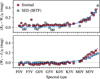Fig. A.1 Comparison of intrinsic color indices derived from synthetic photometry of IRTF spectra (blue points) and from the Simbad database (red points) for dwarf stars. The upper panel shows KS − W1 and the lower panel W1 − I1 as a function of spectral type. The solid lines indicate power-law fits to the distributions.

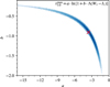Fig. A.2 Distribution of best-fit parameters a and b in the empirical calibration of the ice color excess method, specifically Λ(W1 − I1) (see Eq. (16)), based on 105 random fitting realizations. The color scale indicates the density of solutions with darker shades of blue indicating higher density. The geometric median is marked by a red cross and is adopted as the best-fit solution.

Table A.1 lists the intrinsic infrared colors for a range of spectral types, derived from synthetic photometry of IRTF spectra. These values are crucial for accurately determining the color excess attributable to interstellar ices, as discussed in Sect. 3.2. The table lists intrinsic colors for spectral type F0 through M9 for the colors K_S − W₁, W₁ − I₁, and W₁ − L′. Each color is divided into two sub-columns where the left value corresponds to colors for dwarfs (luminosity class V) and the value on the right corresponds to giants (luminosity class III).

Table A.2 presents the master calibration sample which contains information for the 56 sources used to fit ${\tau }_{3.0}^{max}$ as a function of Λ(W₁ − I₁). For each star, the table provides coordinates, photometric measurements, adopted spectral type, extinction values, measured ice color excess, and literature references.

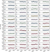Fig. A.3 Time series light curves in the unWISE W1 band for all 56 sources in the calibration sample. Each panel shows the difference between the unTimely and the unWISE mean magnitude in the W1 filter as a function of the observing date, demonstrating the photometric variability over the decade-long baseline. The shaded region indicates the inter-quartile range used for the variability quality cut. The source identification number in the top left of each subplot refers to Table A.2 and the symbol colors and shapes are those listed in Table 1.

A.1 Rotated long tables in appendices

References

All Tables

All Figures

Fig. 1 Infrared passbands and SEDs. The upper panel illustrates transmission curves for the infrared passbands KS, W1, I1, L′, I2, and W2. The lower panel presents the SEDs of three distinct sources: the light blue line represents an X-shooter spectrum of source 15 (refer to Table A.2), the solid red line corresponds to the source NIR38, and the black line depicts Vega. All spectra have been rescaled to facilitate a better comparison.

In the text

Fig. 2 Extinction curves normalized to their value at the effective wavelength of the W1 passband. The different lines correspond to various dust models and R(V) values, as indicated in the legend. WD01 refers to the models of Weingartner & Draine (2001), and D03 to those of Draine (2003). The curves illustrate how both the choice of dust model and R(V) parameter affect the wavelength dependence of extinction.

In the text

Fig. 3 Intrinsic colors for dwarfs (blue symbols) and giants (red symbols) as a function of spectral type, derived from synthetic photometry of IRTF spectra. Solid lines indicate power-law fits to the intrinsic colors for dwarfs (blue) and giants (red), respectively. The upper panel shows intrinsic KS − W1 color, while the lower panel displays W1 − I1. For both color indices, significant deviations from 0 mag are observed only for late spectral types (later than approximately M0).

In the text

Fig. 4 Normalized absorption profiles of the 3 μm feature toward two background stars published by Boogert et al. (2011) and McClure et al. (2023) and one protostar (Rocha et al. 2025) compared with laboratory ice spectra from Hudgins et al. (1993). The observed profiles (red, blue, and green) were extracted from published data and interpolated onto a common wavelength grid. Laboratory spectra correspond to pure water ice (dotted black) and a strong ice mixture (solid black) at 10 K. All profiles are normalized to a peak optical depth of 1 for a direct comparison of the profile shape.

In the text

Fig. 5 Standard deviation (solid lines) and maximum difference (dashed lines) in KS − W1 (black) and W1 − I1 (red) colors as a function of the peak optical depth of the 3 μm feature, calculated for five absorption profiles (see Fig. 4). The KS − W1 color is significantly more sensitive to variations in the absorption profile, while W1 − I1 remains comparatively stable, enabling robust measurements of ${\tau }_{3.0}^{max}$.

In the text

Fig. 6 Standard deviation of Λ and Q′ color excess measurements as a function of the peak optical depth of the 3 μm feature, derived from randomly sampling uncertainties in the photometric parameters and the extinction law. Solid lines represent Λ for different band combinations: Λ(KS − W1) in black, Λ(W1 − I1) in red, and Λ(W1 − L′) in blue. Dashed lines show Q′ for the combinations Q′(KS, W1, I1) (gray) and Q′(KS, W1, L′) (dark blue). The simulation demonstrates that Λ(W1 − I1) and Λ(W1 − L′) maintain the lowest total uncertainties, even at high optical depths, due to the small wavelength separation between the bands.

In the text

	Fig. 7 Positions of the final literature sample of background stars with spectroscopically measured 3 μm optical depths, overlaid on a Planck 857 GHz (350 μm) image of the Milky Way. Different symbols (colors and shapes) indicate the data source, as detailed in Table 1. The sample spans more than 180 deg in Galactic longitude, covering a diverse set of nearby star-forming regions.
In the text

Fig. 8 Peak optical depth of the 3 μm ice absorption feature (${\tau }_{3.0}^{max}$) as a function of the ice color excess Λ(W1 − I1) for the calibration sample. The various symbols represent the different literature sources listed in Table 1. Each point represents a literature measurement with propagated uncertainties. The black dashed line shows the best-fit relation, while thin solid lines represent 500 random samples from the fit parameter space. Gray dashed lines mark ${\tau }_{3.0}^{max}$ = 0 and Λ(W1 − I1) = 0.

In the text

Fig. 9 Relation between the peak optical depth of the 3.0 μm ice feature (${\tau }_{3.0}^{max}$) and the ice color excess Λ(W1 − I1) for different assumptions about the extinction law. The fitted curves correspond to extinction laws from Weingartner & Draine (2001) (blue), Draine (2003) (red), and Boogert et al. (2011) (black). While the use of the Λ(W1 − I1) metric minimizes the impact of extinction law uncertainties, systematic differences between the fits remain visible. However, these differences are generally within the typical measurement uncertainties of the calibration. This highlights the importance of adopting a consistent extinction law or recalibrating the method when applying it to different environments.

In the text

	Fig. A.1 Comparison of intrinsic color indices derived from synthetic photometry of IRTF spectra (blue points) and from the Simbad database (red points) for dwarf stars. The upper panel shows KS − W1 and the lower panel W1 − I1 as a function of spectral type. The solid lines indicate power-law fits to the distributions.
In the text

	Fig. A.2 Distribution of best-fit parameters a and b in the empirical calibration of the ice color excess method, specifically Λ(W1 − I1) (see Eq. (16)), based on 105 random fitting realizations. The color scale indicates the density of solutions with darker shades of blue indicating higher density. The geometric median is marked by a red cross and is adopted as the best-fit solution.
In the text

Fig. A.3 Time series light curves in the unWISE W1 band for all 56 sources in the calibration sample. Each panel shows the difference between the unTimely and the unWISE mean magnitude in the W1 filter as a function of the observing date, demonstrating the photometric variability over the decade-long baseline. The shaded region indicates the inter-quartile range used for the variability quality cut. The source identification number in the top left of each subplot refers to Table A.2 and the symbol colors and shapes are those listed in Table 1.

In the text

References

- Alves, J., Lombardi, M., & Lada, C. J. 2025, A&A, 697, A208 [NASA ADS] [CrossRef] [EDP Sciences] [Google Scholar]
- Astropy Collaboration (Robitaille, T. P., et al.) 2013, A&A, 558, A33 [NASA ADS] [CrossRef] [EDP Sciences] [Google Scholar]
- Astropy Collaboration (Price-Whelan, A. M., et al.) 2018, AJ, 156, 123 [Google Scholar]
- Astropy Collaboration (Price-Whelan, A. M., et al.) 2022, ApJ, 935, 167 [NASA ADS] [CrossRef] [Google Scholar]
- Baratta, G. A., & Strazzulla, G. 1990, A&A, 240, 429 [Google Scholar]
- Benjamin, R. A., Churchwell, E., Babler, B. L., et al. 2003, PASP, 115, 953 [Google Scholar]
- Bohlin, R. C., Gordon, K. D., & Tremblay, P. E. 2014, PASP, 126, 711 [NASA ADS] [Google Scholar]
- Bonnarel, F., Fernique, P., Bienaymé, O., et al. 2000, A&AS, 143, 33 [NASA ADS] [CrossRef] [EDP Sciences] [Google Scholar]
- Boogert, A. C. A., Huard, T. L., Cook, A. M., et al. 2011, ApJ, 729, 92 [NASA ADS] [CrossRef] [Google Scholar]
- Boogert, A. C. A., Chiar, J. E., Knez, C., et al. 2013, ApJ, 777, 73 [NASA ADS] [CrossRef] [Google Scholar]
- Boogert, A. C. A., Gerakines, P. A., & Whittet, D. C. B. 2015, ARA&A, 53, 541 [Google Scholar]
- Chiar, J. E., Pendleton, Y. J., Allamandola, L. J., et al. 2011, ApJ, 731, 9 [NASA ADS] [CrossRef] [Google Scholar]
- Crill, B. P., Werner, M., Akeson, R., et al. 2020, SPIE Conf. Ser., 11443, 114430I [Google Scholar]
- Cutri, R. M., Wright, E. L., VizieR On-line Data Catalog: II/328 [Google Scholar]
- Danielson, R. E., Woolf, N. J., & Gaustad, J. E. 1965, ApJ, 141, 116 [Google Scholar]
- Dartois, E., Noble, J. A., Caselli, P., et al. 2024, Nat. Astron., 8, 359 [NASA ADS] [CrossRef] [Google Scholar]
- Draine, B. T. 2003, ARA&A, 41, 241 [NASA ADS] [CrossRef] [Google Scholar]
- Evans, II, N. J., Allen, L. E., Blake, G. A., et al. 2003, PASP, 115, 965 [CrossRef] [Google Scholar]
- Fazio, G. G., Hora, J. L., Allen, L. E., et al. 2004, ApJS, 154, 10 [Google Scholar]
- Fouesneau, M. 2025, pyphot, Zenodo, Version pyphot_v1.6.0 [Google Scholar]
- Gaia Collaboration (Prusti, T., et al.) 2016, A&A, 595, A1 [NASA ADS] [CrossRef] [EDP Sciences] [Google Scholar]
- Gaia Collaboration (Vallenari, A., et al.) 2023, A&A, 674, A1 [NASA ADS] [CrossRef] [EDP Sciences] [Google Scholar]
- Gardner, J. P., Mather, J. C., Clampin, M., et al. 2006, Space Sci. Rev., 123, 485 [Google Scholar]
- Gillett, F. C., & Forrest, W. J. 1973, ApJ, 179, 483 [NASA ADS] [CrossRef] [Google Scholar]
- Ginsburg, A., Sipőcz, B. M., Brasseur, C. E., et al. 2019, AJ, 157, 98 [Google Scholar]
- Goodman, A. A., Pineda, J. E., & Schnee, S. L. 2009, ApJ, 692, 91 [Google Scholar]
- Goto, M., Bailey, J. D., Hocuk, S., et al. 2018, A&A, 610, A9 [EDP Sciences] [Google Scholar]
- Green, G. M., Zhang, X., & Zhang, R. 2025, ApJ, 988, 5 [Google Scholar]
- Greene, T. P., Kelly, D. M., Stansberry, J., et al. 2017, J. Astron. Teles. Instrum. Syst., 3, 035001 [Google Scholar]
- Harris, C. R., Millman, K. J., van der Walt, S. J., et al. 2020, Nature, 585, 357 [NASA ADS] [CrossRef] [Google Scholar]
- Hasenberger, B., Lombardi, M., Alves, J., et al. 2018, A&A, 620, A24 [NASA ADS] [CrossRef] [EDP Sciences] [Google Scholar]
- Houck, J. R., Roellig, T. L., van Cleve, J., et al. 2004, ApJS, 154, 18 [NASA ADS] [CrossRef] [Google Scholar]
- Hudgins, D. M., Sandford, S. A., Allamandola, L. J., & Tielens, A. G. G. M. 1993, ApJS, 86, 713 [NASA ADS] [CrossRef] [Google Scholar]
- Hunter, J. D. 2007, Comput. Sci. Eng., 9, 90 [NASA ADS] [CrossRef] [Google Scholar]
- Jakobsen, P., Ferruit, P., Alves de Oliveira, C., et al. 2022, A&A, 661, A80 [NASA ADS] [CrossRef] [EDP Sciences] [Google Scholar]
- Johnson, H. L., & Morgan, W. W. 1953, ApJ, 117, 313 [NASA ADS] [CrossRef] [Google Scholar]
- Knacke, R. F., Cudaback, D. D., & Gaustad, J. E. 1969, ApJ, 158, 151 [Google Scholar]
- Lada, C. J., Lada, E. A., Clemens, D. P., & Bally, J. 1994, ApJ, 429, 694 [NASA ADS] [CrossRef] [Google Scholar]
- Lada, C. J., Lewis, J. A., Lombardi, M., & Alves, J. 2017, A&A, 606, A100 [NASA ADS] [CrossRef] [EDP Sciences] [Google Scholar]
- Lombardi, M. 2018, A&A, 615, A174 [NASA ADS] [CrossRef] [EDP Sciences] [Google Scholar]
- Lombardi, M., & Alves, J. 2001, A&A, 377, 1023 [NASA ADS] [CrossRef] [EDP Sciences] [Google Scholar]
- Lombardi, M., Bouy, H., Alves, J., & Lada, C. J. 2014, A&A, 566, A45 [NASA ADS] [CrossRef] [EDP Sciences] [Google Scholar]
- Madden, M. C. L., Boogert, A. C. A., Chiar, J. E., et al. 2022, ApJ, 930, 2 [NASA ADS] [CrossRef] [Google Scholar]
- Mainzer, A., Bauer, J., Grav, T., et al. 2011, ApJ, 731, 53 [Google Scholar]
- Majewski, S. R., Zasowski, G., & Nidever, D. L. 2011, ApJ, 739, 25 [Google Scholar]
- McClure, M. K., Rocha, W. R. M., Pontoppidan, K. M., et al. 2023, Nat. Astron., 7, 431 [NASA ADS] [CrossRef] [Google Scholar]
- McKinney, W. 2010, in Proceedings of the 9th Python in Science Conference, eds. S. van der Walt, & J. Millman, 56 [Google Scholar]
- Meingast, S., Lombardi, M., & Alves, J. 2017, A&A, 601, A137 [NASA ADS] [CrossRef] [EDP Sciences] [Google Scholar]
- Meingast, S., Alves, J., & Lombardi, M. 2018, A&A, 614, A65 [NASA ADS] [CrossRef] [EDP Sciences] [Google Scholar]
- Meingast, S., Alves, J., Bouy, H., et al. 2023, A&A, 673, A58 [NASA ADS] [CrossRef] [EDP Sciences] [Google Scholar]
- Meisner, A. M., Caselden, D., Schlafly, E. F., & Kiwy, F. 2023, AJ, 165, 36 [NASA ADS] [CrossRef] [Google Scholar]
- Minniti, D., Lucas, P. W., Emerson, J. P., et al. 2010, New A, 15, 433 [Google Scholar]
- Murakawa, K., Tamura, M., & Nagata, T. 2000, ApJS, 128, 603 [Google Scholar]
- Noble, J. A., Fraser, H. J., Aikawa, Y., Pontoppidan, K. M., & Sakon, I. 2013, ApJ, 775, 85 [Google Scholar]
- Noble, J. A., Fraser, H. J., Smith, Z. L., et al. 2024, Nat. Astron., 8, 1169 [NASA ADS] [CrossRef] [Google Scholar]
- Ochsenbein, F. 1996, The VizieR database of astronomical catalogues [Google Scholar]
- Ochsenbein, F., Bauer, P., & Marcout, J. 2000, A&AS, 143, 23 [NASA ADS] [CrossRef] [EDP Sciences] [Google Scholar]
- Ohyama, Y., Onaka, T., Matsuhara, H., et al. 2007, PASJ, 59, S411 [Google Scholar]
- Onaka, T., Matsuhara, H., Wada, T., et al. 2007, PASJ, 59, S401 [Google Scholar]
- Pandas Development Team 2020, https://doi.org/10.5281/zenodo.3509134 [Google Scholar]
- Pedregosa, F., Varoquaux, G., Gramfort, A., et al. 2011, J. Mach. Learn. Res., 12, 2825 [Google Scholar]
- Persson, S. E., Murphy, D. C., Krzeminski, W., Roth, M., & Rieke, M. J. 1998, AJ, 116, 2475 [NASA ADS] [CrossRef] [Google Scholar]
- Pilbratt, G. L., Riedinger, J. R., Passvogel, T., et al. 2010, A&A, 518, L1 [NASA ADS] [CrossRef] [EDP Sciences] [Google Scholar]
- Planck Collaboration I. 2011, A&A, 536, A1 [NASA ADS] [CrossRef] [EDP Sciences] [Google Scholar]
- Pokhrel, R., Gutermuth, R. A., Betti, S. K., et al. 2020, ApJ, 896, 60 [NASA ADS] [CrossRef] [Google Scholar]
- Posch, L., Miret-Roig, N., Alves, J., et al. 2023, A&A, 679, L10 [NASA ADS] [CrossRef] [EDP Sciences] [Google Scholar]
- Ratzenböck, S., Großschedl, J. E., Alves, J., et al. 2023, A&A, 678, A71 [NASA ADS] [CrossRef] [EDP Sciences] [Google Scholar]
- Rayner, J. T., Toomey, D. W., Onaka, P. M., et al. 2003, PASP, 115, 362 [NASA ADS] [CrossRef] [Google Scholar]
- Rebull, L. M., Padgett, D. L., McCabe, C. E., et al. 2010, ApJS, 186, 259 [NASA ADS] [CrossRef] [Google Scholar]
- Rocha, W. R. M., McClure, M. K., Sturm, J. A., et al. 2025, A&A, 693, A288 [NASA ADS] [CrossRef] [EDP Sciences] [Google Scholar]
- Rodrigo, C., & Solano, E. 2020, in XIV. 0 Scientific Meeting (virtual) of the Spanish Astronomical Society, 182 [Google Scholar]
- Rodrigo, C., Solano, E., & Bayo, A. 2012, SVO Filter Profile Service Version 1.0, IVOA Working Draft 15 October 2012 [Google Scholar]
- Schlafly, E. F., Meisner, A. M., & Green, G. M. 2019, ApJS, 240, 30 [Google Scholar]
- Simons, D. A., & Tokunaga, A. 2002, PASP, 114, 169 [Google Scholar]
- Skrutskie, M. F., Cutri, R. M., Stiening, R., et al. 2006, AJ, 131, 1163 [NASA ADS] [CrossRef] [Google Scholar]
- Smith, R. G., Sellgren, K., & Brooke, T. Y. 1993, MNRAS, 263, 749 [NASA ADS] [CrossRef] [Google Scholar]
- Smith, Z. L., Dickinson, H. J., Fraser, H. J., et al. 2025, Nature Astronomy, 9, 883 [Google Scholar]
- Swiggum, C., Alves, J., Benjamin, R., et al. 2024, Nature, 631, 49 [NASA ADS] [CrossRef] [Google Scholar]
- Taurus Team 2020, Taurus 2: Finishing the Spitzer Map of the Taurus Molecular Clouds, NASA IPAC DataSet, IRSA434 [Google Scholar]
- Tielens, A. G. G. M., Allamandola, L. J., Bregman, J., et al. 1984, ApJ, 287, 697 [Google Scholar]
- Vernet, J., Dekker, H., D’Odorico, S., et al. 2011, A&A, 536, A105 [NASA ADS] [CrossRef] [EDP Sciences] [Google Scholar]
- Virtanen, P., Gommers, R., Oliphant, T. E., et al. 2020, Nat. Methods, 17, 261 [Google Scholar]
- Weingartner, J. C., & Draine, B. T. 2001, ApJ, 548, 296 [Google Scholar]
- Wenger, M., Ochsenbein, F., Egret, D., et al. 2000, A&AS, 143, 9 [NASA ADS] [CrossRef] [EDP Sciences] [Google Scholar]
- Werner, M. W., Roellig, T. L., Low, F. J., et al. 2004, ApJS, 154, 1 [NASA ADS] [CrossRef] [Google Scholar]
- Wright, E. L., Eisenhardt, P. R. M., Mainzer, A. K., et al. 2010, AJ, 140, 1868 [Google Scholar]
- Zari, E., Lombardi, M., Alves, J., Lada, C. J., & Bouy, H. 2016, A&A, 587, A106 [NASA ADS] [CrossRef] [EDP Sciences] [Google Scholar]
- Zhang, X., & Green, G. M. 2025, Science, 387, 1209 [Google Scholar]
- Zhang, M., & Kainulainen, J. 2022, MNRAS, 517, 5180 [NASA ADS] [CrossRef] [Google Scholar]
In this manuscript, I refer to the first (i.e., bluest) passbands of the WISE and Spitzer missions as W1 and I1, corresponding to the WISE1 and IRAC1 filters, respectively. Details on passbands and transmission curves are taken from the Spanish Virtual Observatory (SVO) Filter Profile Service (Rodrigo et al. 2012; Rodrigo & Solano 2020).