| Issue |
A&A
Volume 702, October 2025
|
|
|---|---|---|
| Article Number | A126 | |
| Number of page(s) | 15 | |
| Section | Interstellar and circumstellar matter | |
| DOI | https://doi.org/10.1051/0004-6361/202555862 | |
| Published online | 10 October 2025 | |
MINDS: A transition from H2O to C2H2 dominated disk spectra with decreasing stellar luminosity
1
Max-Planck-Institut für Extraterrestrische Physik,
Giessenbachstrasse 1,
85748
Garching,
Germany
2
Earth and Planets Laboratory, Carnegie Institution for Science,
5241 Broad Branch Road,
NW,
Washington,
DC 20015,
USA
3
Leiden Observatory, Leiden University,
PO Box 9513,
2300 RA
Leiden,
The Netherlands
4
Institute of Astronomy, KU Leuven,
Celestijnenlaan 200D,
3001
Leuven,
Belgium
5
Kapteyn Astronomical Institute, Rijksuniversiteit Groningen,
Postbus 800,
9700AV
Groningen,
The Netherlands
6
Université Paris-Saclay, CNRS, Institut d’Astrophysique Spatiale,
91405
Orsay,
France
7
Max-Planck-Institut für Astronomie (MPIA),
Königstuhl 17,
69117
Heidelberg,
Germany
8
INAF – Osservatorio Astronomico di Capodimonte,
Salita Moiariello 16,
80131
Napoli,
Italy
9
Dublin Institute for Advanced Studies,
31 Fitzwilliam Place,
D02 XF86
Dublin,
Ireland
10
STAR Institute, Université de Liège,
Allée du Six Août 19c,
4000
Liège,
Belgium
11
Dept. of Astrophysics, University of Vienna,
Türkenschanzstr. 17,
1180
Vienna,
Austria
12
ETH Zürich, Institute for Particle Physics and Astrophysics,
Wolfgang-Pauli-Str. 27,
8093
Zürich,
Switzerland
13
Department of Astrophysics/IMAPP, Radboud University,
PO Box 9010,
6500 GL
Nijmegen,
The Netherlands
14
Department of Physics and Astronomy, University of Exeter,
Exeter
EX4 4QL,
UK
15
Centro de Astrobiología (CAB), CSIC-INTA, ESAC Campus, Camino Bajo del Castillo s/n, 28692 Villanueva de la Cañada,
Madrid,
Spain
16
Niels Bohr Institute, University of Copenhagen,
NBB BA2, Jagtvej 155A,
2200
Copenhagen,
Denmark
17
SRON Netherlands Institute for Space Research,
Niels Bohrweg 4,
2333 CA
Leiden,
The Netherlands
★ Corresponding author: This email address is being protected from spambots. You need JavaScript enabled to view it.
Received:
7
June
2025
Accepted:
5
August
2025
Abstract
Context. The chemical composition of the inner regions of disks around young stars will largely determine the properties of planets that form in these regions. Many physical processes in the disks drive their chemical evolution, and some of them depend on and/or correlate with the stellar properties.
Aims. We explore the connection between stellar properties and the chemistry of the inner disk in protoplanetary disks as traced by mid-infrared spectroscopy.
Methods. We used JWST-MIRI observations of a large diverse sample of sources to explore trends between the carbon-bearing molecule C2H2 and the oxygen-bearing molecule H2O. Additionally, we calculated the average spectrum for the T Tauri (M*>0.2 M⊙) and very low-mass star (VLMS; M*,≤0.2 M⊙) samples from JWST-MIRI MRS data and used slab models to determine the properties of the average spectra in each subsample.
Results. We find a significant anticorrelation between the flux ratio of C2H2/H2O and the stellar luminosity. The FC2H2/FH2O flux ratios of disks around VLMSs are significantly higher than the fluxes in their higher-mass counterparts. This is driven by the generally weak H2O and strong C2H2 in disks around low-mass hosts. We also explored trends with the strength of the 10 µm silicate feature, the stellar accretion rate, and the disk dust mass. They are all correlated with FC2H2/FH2O, which may be related to processes that drive the carbon enrichment in disks around VLMSs, but are also degenerate with the system properties (i.e., the M*−Ṁ and M*−Mdisk relations). Slab model fits to the average spectra show that H2O emission in the VLMS sample is quite similar in temperature and column density to a warm (~600 K) H2O component in the T Tauri spectrum. This indicates that the high C/O gas-phase ratio in these disks is not due to oxygen depletion alone. Instead, the many hydrocarbons, including some with high column densities, suggest that carbon enhancement occurs in the disks around VLMSs.
Conclusions. The observed differences in the chemistry of the inner disk as a function of host properties are likely to be accounted for by differences in the disk temperatures, stellar radiation field, and the evolution of dust grains.
Key words: planets and satellites: formation / protoplanetary disks / stars: pre-main sequence
© The Authors 2025
 Open Access article, published by EDP Sciences, under the terms of the Creative Commons Attribution License (https://creativecommons.org/licenses/by/4.0), which permits unrestricted use, distribution, and reproduction in any medium, provided the original work is properly cited.
This article is published in open access under the Subscribe to Open model.
Open Access funding provided by Max Planck Society.
1 Introduction
Understanding the main factors that affect the chemistry of a protoplanetary disk is very important for understanding the conditions during planet formation, and therefore, for constraining the available material for nascent rocky and giant planets (e.g., Öberg & Bergin 2021). The vertical and radial evolution and structure of the dust disk and the stellar luminosity, which controls the disk temperature, are expected to strongly affect the gaseous composition of the inner regions of disks in which terrestrial planets form. Infrared spectroscopy is a critical tool for determining the molecules in these inner few au of proto-planetary disks, but also for determining the conditions of the gas and the processes that set the chemistry. Observations with the Infrared Space Observatory Spitzer and now with the James Webb Space Telescope (JWST) provide a unique window into these inner disk regions, and the sensitivity and spectral resolution of JWST grants us new understandings of the first stages of planet formation.
Large and diverse samples of protoplanetary disks have been observed in the mid-infrared, and trends between the chemistry and the physical properties of these systems can be investigated. This provides a way to determine the factors that drive the chemistry. Large samples observed with Spitzer using the Infrared Spectrograph (IRS) provided great insight into the links between the inner disk chemistry with overall disk properties (e.g., Pontoppidan et al. 2014). For instance, a trend was found between the flux ratio of HCN/H2O and the disk mass, which might indicate that more massive disks lock up oxygen-rich ices in the cold outer regions and deprive the inner disk of H2O enrichment (Najita et al. 2013). This conclusion was reinforced by trends found between the H2O/HCN flux ratio and the disk dust radius, with smaller disks having more H2O than HCN (Banzatti et al. 2020). Trends were also found as a function of the stellar properties, largely the stellar mass and luminosity. Pascucci et al. (2009, 2013) found that cool stars (spectral type later than M5) have very different chemical signatures in the mid-infrared than earlier-type stars (spectral type between K1 and M5), with the cool stars having higher C2H2 fluxes than HCN, where the opposite is true for earlier-type stars. These trends provided key insights into the impact of disk evolution and stellar properties on setting the chemistry of the inner disk and were only possible by access to large diverse observational samples.
The results from the JWST build on the legacy of Spitzer in the study of the inner regions of protoplanetary disks. The increased sensitivity and spectral resolution of JWST-MIRI compared to Spitzer-IRS allows us to detect isotopologs (e.g., Grant et al. 2023; Tabone et al. 2023; Salyk et al. 2025), to de-blend rovibrational and pure rotational H2O lines (e.g., Pontoppidan et al. 2024; Gasman et al. 2023), and to detect very weak emission to reveal previously unknown molecular content (e.g., Perotti et al. 2023; Arabhavi et al. 2024, 2025b). These advancements, along with the analysis of increasingly large samples (e.g., Romero-Mirza et al. 2024; Arabhavi et al. 2025a; Arulanantham et al. 2025; Banzatti et al. 2025), transform our understanding of the chemistry in the inner disk by allowing us to account better for the chemical complexity. This provides tighter constraints on the gas properties. We can also explore the relations with the system properties.
We studied a large sample of disks observed with JWST-MIRI MRS and determined a strong anti-correlation between the C2H2/H2O flux ratio and the stellar luminosity that spans three orders of magnitude in stellar luminosity (and two orders of magnitude in stellar mass, including the transition from the stellar to substellar regimes) and over three orders of magnitude in flux ratio. In Section 2 we present the sample, observations, and methods we used to calculate the line fluxes and dust properties. In Section 3 we present the anticorrelations between  and the stellar luminosity, accretion rate, disk dust mass, and the strength of the 10 µm silicate feature and the average spectrum for the T Tauri and VLMS samples, as well as a slab model fit to these average spectra. We discuss these results and the degeneracies between many of the system parameters in Section 4. We provide a summary of our findings in Section 5.
2 Sample, observations, and methods
2.1 Sample
Our sample comes from the Mid-INfrared Disk Survey (MINDS) JWST guaranteed time program (PID 1282, PI: Henning, Henning et al. 2024; Kamp et al. 2023). The entire MINDS sample consists of 52 targets that span stellar masses from the substellar brown dwarf regime to Herbig Ae stars and five debris disks. We did not include debris disks, highly inclined sources, Herbig Ae/Be systems, or sources dominated by polycyclic aromatic hydrocarbon emission in our analysis. We also included the brown dwarf system TWA 27A/2MASS J12073346-3932539 from PID 1270 (PI: Birkmann; see Patapis et al. 2025). For this work, the T Tauri sample is taken to be objects with a stellar mass above 0.2 M⊙, while the VLMS sample is taken as objects with host masses of 0.2 M⊙ and below, including objects in the brown dwarf regime. Our sample thus consists of nine very low-mass stars and brown dwarfs (M* ~ 0.02 to 0.16 M⊙, SpT from M4.5 to M9; see Arabhavi et al. 2025a for more details on this sample) and 25 T Tauri stars (M* ~ 0.25 to 1.5 M⊙, SpT from M4 to G8). All of these sources were observed with the Mid-Infrared Instrument (MIRI) in the medium-resolution mode (MRS; Wright et al. 2023). This provided spectra from 4.9 to 28 µm at a resolving power of R ~ 1500–3500.
The stellar and disk properties for our sample were collected from the literature and are provided in Table 1. The accretion rate and disk dust masses were taken from the compilation of Manara et al. (2023).
2.2 JWST observations and data reduction
The entire sample was reduced using the standard pipeline reduction (version 1.16.1; Bushouse et al. 2024) and pmap 1315. Aperture photometry with an aperture size of twice the full width at half maximum was used to extract the spectra. Residual fringes were removed using the default pipeline. The reduced spectra for all of the targets analyzed in this work are made publicly available1.
Continuum-subtraction was made following the methods of Temmink et al. (2024b). Briefly, this was done via an iterative fitting in which the continuum was fit using a Savitzky-Golay filter with a third-order polynomial. Emission lines above 2σ above the continuum were masked to avoid skewing the continuum estimation. The continuum was then subtracted, and all downward spikes more than 3σ below the continuum were masked. Finally, the baseline was determined using PyBaselines (Erb 2022). Molecular pseudo-continuum is present in all of the VLMSs. For these sources, the wavelength ranges where the pseudo-continua were clearly present were masked by eye from the continuum determination.
2.3 Line fluxes
The H2O flux was determined by integrating the spectrum over three windows centered on lines with upper energy levels of 2400 to 6000 K and Einstein A coefficients of 1 to 42 s−1 in the 17 µm range: 17.09-17.15 µm, 17.2–17.245 µm, and 17.3–17.42 µm. These transitions, and thus the integrated flux that we measured, largely trace a warm H2O component, with a temperature of ~400 K. However, H2O has been found to have gradients in temperature in disks (e.g., Temmink et al. 2024a; Gasman et al. 2023; Banzatti et al. 2023; Grant et al. 2024; Muñoz-Romero et al. 2024), and we therefore only trace a portion of the H2O in these systems. Some may have different reservoirs of hot and cold water. These lines are more commonly detected for the VLMS sample than hot ro-vibrational lines at shorter wavelengths, however, and are less strongly blended with hydrocarbon features between ~12 and 16 µm. Finally, the noise level is too high to access the very cold components at ~24 µm (Arabhavi et al. 2025b).
In H2O-rich spectra, H2O lines can contaminate the C2H2 Q-branch at 13.7 µm. We therefore followed the methods of Banzatti et al. (2020) to remove the H2O contribution before we determined the C2H2 flux. We took a local thermodynamic equilibrium H2O slab model with a temperature of 600 K and a column density of 1018 cm−2 (properties that were found for H2O lines near the C2H2 feature; e.g., Grant et al. 2023; Gasman et al. 2023), and we scaled it to match the continuum and peak fluxes of the water lines in two windows (13.415–513.445 µm and 14.19–14.35 µm) close in wavelength to the C2H2 Q-branch peak. This H2O model was then subtracted from the observed spectrum before the integrated C2H2 flux was measured. We note that it was not necessary to remove the H2O emission for the VLMSs because the H2O emission is very weak, if present at all. Any fit for H2O will be greatly contaminated by the strong C2H2 and HCN emission. The C2H2 flux was integrated from 13.60 to 13.72 µm.
To determine whether H2O and C2H2 are detected requires understanding the noise level in the spectrum. This can be very challenging in the line-rich MIRI spectra because there is little pure continuum on which to measure the noise level. Based on model spectra of the common molecular species found in the 13 to 18 µm wavelength range, we selected wavelength regions that contained the least molecular emission in which to determine the noise (from 15.895 to 15.91 µm for the T Tauris and 16.375 and 16.395 µm for the VLMSs). The species was considered detected when the line flux was greater than 3σ. In several cases, the spectra are very line rich or are noisy, however, which led to 3σ detections that were not reliable when inspected by eye. For instance, the integrated flux over the C2H2 feature is high, but the region has residual water lines and/or no discernible C2H2 Q-branch. In these cases, we considered these nondetections, but provide the 3σ upper limits in Table 1. Finally, while we used the 3σ threshold, confirmed by visual inspection, to determine whether the emission was detected in this work, H2O was detected in most of the VLMSs through a cross-correlation, either at shorter wavelengths or in the rotational lines that we analyzed here. We refer to Arabhavi et al. (2025b) for details on these H2O detections in the VLMS sample.
Stellar properties and line fluxes.
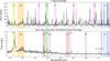 |
Fig. 1 Average T Tauri (top) and VLMS (bottom) sample JWST spectra. The detected molecular species are highlighted. The C2H2 and H2O regions (yellow and blue, respectively) show the regions over which the fluxes were integrated. Most of the unlabeled lines in the T Tauri average are various H2O transitions. |
2.4 10 µm silicate feature strength
In order to investigate the connection between the gas properties and the (infrared) dust properties, we calculated the strength of the 10 µm silicate feature following the methods of van Boekel et al. (2003); Kessler-Silacci et al. (2006), for example. F9.8 = 1 + (f9.8,cs/ < fc >), where f9.8,cs is the spectrum after subtracting the continuum that is determined by two anchor points, one point from 6.8 to 7.5 µm and the other point from 12.5 to 13.5 µm, and < fc > is the mean of the continuum. For four of the VLMSs (2MASS J16053215-1933159, 2MASS J11071860-7732516, 2MASS J11082650-7715550, and 2MASS J12073346-3932539), there is either no 10 µm emission or any emission around 10 µm comes at least partially from optically thick C2H4 (Arabhavi et al. 2024, 2025a). For these sources, we therefore adopted a band strength of one, which is representative of no silicate emission.
3 Results
3.1 Average spectrum
To explore the properties of the T Tauri and VLMS samples, we took the average spectrum of each sample to perform a spectral fit. Each spectrum was scaled to a common distance of 120 pc before the spectra were averaged in each wavelength bin. The average spectra of the T Tauri and VLMS samples are presented in Figure 1. This figure clearly highlights the difference in the molecular emission between the two samples. The H2O lines are the strongest features in the averaged T Tauri spectrum, followed by the CO2 and HCN Q-branches, OH, and finally, C2H2. By comparison, the averaged VLMS spectrum is dominated by the bright C2H2 Q-branch, followed by C6H6, HCN, CO2, C4H2, HC3N, 13CO2, and finally, H2O is the weakest feature.
3.2 The flux ratio of C2H2 and H2O
The anticorrelation between  (identically
  ) and the stellar luminosity is shown in Figure 2. This correlation spans over three orders of magnitude in stellar luminosity (almost two orders of magnitude in stellar mass) and over three orders of magnitude in
  . The absolute flux of H2O decreases with decreasing stellar luminosity (Pearson correlation coefficient, PCC=0.84, p-value=6×10⁻¹⁰), but the C2H2 flux does not; instead, the C2H2 line-to-continuum ratio increases with decreasing stellar luminosity (PCC=−0.65, p-value=2.7×10⁻⁵; see Figure A.1 in Appendix A and also Figure 8 in Arabhavi et al. 2025b). Therefore, the strong correlation we found between
  and L* (PCC=−0.77, p-value=1.3×10⁻⁷) is due to a combination of weak H2O and strong C2H2 features in the very low-mass objects and vice versa for the T Tauri stars. While
  decrease overall with increasing stellar luminosity, even at a given stellar luminosity in the T Tauri sample, the spread in line flux ratio is ~50. We did not include the accretion luminosity in the luminosity plotted in Figure 2 because the stellar luminosity is much higher (Lacc≲0.1L* or even Lacc≲0.01* for the range of stellar luminosities in our sample; e.g., Mendigutía et al. 2015; Alcalá et al. 2017; Manara et al. 2017). We note, however, that this would only strengthen the correlation, if only modestly.
Additional correlations are seen with other system properties, including the stellar mass, accretion rate, and disk dust mass (the latter two are presented in Figure 3). Given the correlations between stellar luminosity and mass and the correlations of the other properties with stellar mass (M*,−Ṁ as in, e.g., Hillenbrand et al. 1992; Hartmann et al. 2016; Grant et al. 2022; Manara et al. 2023 and M*−Mdust as in, e.g., Andrews et al. 2013; Pascucci et al. 2016; Manara et al. 2023), this is not surprising. The trends seen with these system parameters are not as strong as the trend with stellar luminosity. It would also be interesting to place the JWST results into context with the outer disk information, but high-resolution (sub-)millimeter observations of the VLMS sample are currently lacking, and we therefore cannot explore any potential correlations with Rdisk (but see Arulanantham et al. 2025 for the JWST Disk Infrared Spectral Chemistry Survey sample of T Tauri objects). We discuss the potential role of radial drift further in Section 4.
In Figure 3 we also show the relation between  and the strength of the 10 µm silicate feature. An overall negative correlation is observed, that is, targets with weaker silicate features are more likely to have stronger C2H2 emission relative to H2O. Interestingly, none of the sources with a 10 µm band strength greater than 1.85 have C2H2 detections. The potential underlying connection is discussed in Section 4.3. Correlations between the parameters discussed above are also provided relative to the absolute fluxes and to the line-to-continuum ratios in Appendix A, where the strongest correlation is between the H2O flux and the accretion rate, as was found previously (e.g., Banzatti et al. 2020).
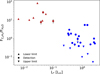 |
Fig. 2 Relation between the flux ratio of C2H2 to H2O as a function of stellar luminosity. Objects with M*>0.2 M⊙ are shown in blue and represent our T Tauri sample, and those with stellar masses below 0.2 M⊙ are our VLMS sample and are shown in red. The two outliers around L* ~ 1 L⊙ are DL Tau and V1094 Sco, which will be analyzed in detail in Tabone et al. (in prep.). This trend is statistically significant with a p-value of 1.3×10⁻⁷ and a correlation coefficient of −0.77. 3σ upper and lower limits are the downward and upward triangles, respectively. The error bars are smaller than the points for most targets. |
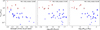 |
Fig. 3 Left: |


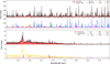 |
Fig. 4 Average spectra for disks in our T Tauri sample (top) and VLMS sample (bottom) in black, compared to the best-fit model in red. The model components are shown below each for reference. |
3.3 Fitting the average spectra
In order to interpret the average properties, we used 0D LTE slab models (see Grant et al. 2023; Tabone et al. 2023 for details) to reproduce the average spectra using only three free parameters: the column density (N), the temperature (T), and the emitting area, which is characterized by a disk with an emitting radius (R). In order to fit each spectrum, we followed the method of Grant et al. (2023). Briefly, the slab model spectra were calculated with a Gaussian line profile with a full width at half maximum of ΔV = 4.7 km s−1 (σ = 2 km s−1) at a spectral resolving power of 2300 to match the resolution of MIRI MRS in the ~ 13 to 17 µm wavelength region. Then, the model was sampled on the same wavelength grid as the data using SpectRes (Carnall 2017). A grid of models was calculated for each molecular species, with N from 1014 to 1022 cm−2 in steps of 0.166 in log10-space, T from 100 to 1500 K in steps of 25 K, and the emitting area was varied by changing the radius from 0.001 to 10 au in steps of 0.02 in log10-space. One molecule was fit at a time in wavelength regions that were relatively devoid of emission from other species. Then, the best-fit model was subtracted, and the next species was fit. This iterative approach has been shown to produce consistent results with an analysis performed by simultaneously fitting all molecular species (e.g., Grant et al. 2023 and Kaeufer et al. 2024a). Two H2O components, one hot component with T>1000 K and one intermediate component with T ~ 600 K, were needed to reproduce the lines in the 13–17.5 µm wavelength range for the average T Tauri spectrum, which agrees with works on individual sources (e.g., Grant et al. 2024; Temmink et al. 2024a; Romero-Mirza et al. 2024; Banzatti et al. 2025). Similarly, two components were needed to fit the C2H2 in the VLMS spectrum in order to reproduce the molecular pseudo-continuum (Tabone et al. 2023; Arabhavi et al. 2024; Kanwar et al. 2024). The best-fit model is shown in Figure 4, and the best-fit properties for the molecules that are present in the average VLMS and T Tauri spectra are presented in Figure 5. The χ2 maps are presented in Figures B.1 and B.2 for the T Tauri and VLMS spectra, respectively.
While some of the molecules are only poorly constrained, we drew some interesting conclusions from the average-fit properties. Notably, the column densities for HCN, CO2, and H2O (the intermediate component for the T Tauri spectrum) are consistent between the VLMS and the T Tauri objects. While the equivalent emitting radii are largely unconstrained because the radii and column density are degenerate in the optically thin regime, the radii tend to lower values in the VLMSs than in the T Tauris stars. The locations of the snowline in the disks around VLMSs are different from those in T Tauri stars. We therefore determined the location of the water snowline for each subsample in order to normalize the emitting radii in the bottom right panel of Figure 5. We used Equation (2) in Mulders et al. (2015) to determine the snowline location, which is based on the 3D radiative transfer models of Min et al. (2011), using the average stellar mass and accretion rate for each subsample (M* ~ 0.6 M⊙ and Ṁ ~ 10−7.75 M⊙ yr−1 for the T Tauri sample and M* ~ 0.08 M⊙ and Ṁ ~ 10¯10 M⊙ yr−1 for the VLMS sample). This resulted in a location of the H2O snowline of 2.25 and 0.12 au for the T Tauris and VLMS stars, respectively. With this normalization, the gas properties of the VLMS tend to have larger emitting radii than their higher-mass counterparts. One of the most well-constrained molecules in each case is CO2 which is optically thick for both samples and has a cooler temperature than the other molecules. Our CO2 and C2H2 temperatures are colder than what was found in the JDISCS sample of Arulanantham et al. (2025). Although it will be necessary to model each spectrum to obtain a more global picture of the diversity in the molecular properties (as was done in Arulanantham et al. 2025), the average fit already provides interesting initial clues for the similarities and differences between the two samples.
While not shown in Figure 5, the hydrocarbons in addition to C2H2 in the VLMS spectra tend to be cold (<300 K) and in the optically thin regime, with column densities ≲10−17.5 cm−2 (see Figure B.2). The difference in temperature between C2H2 and the other hydrocarbons is likely due at least in part to the high abundances of C2H2. The optically thick component likely originates in the very inner disk, given its small emitting area, as recently observed in several sources (Tabone et al. 2023; Arabhavi et al. 2024; Kanwar et al. 2024; Long et al. 2025). Based on the 1σ contours for the equivalent emitting radius, the maximum radius for the optically thick C2H2 component is 2.5 times smaller than the minimum radius for the optically thin component (0.027 versus 0.067 au, respectively). Although we cannot place good constraints on the emitting area of the optically thin hydrocarbon emission (see Figure B.2), the higher temperature of the optically thin C2H2 component compared to the other more complex hydrocarbons might arise because it emits at higher layers in the disk atmosphere (see Appendix D in Kanwar et al. 2024) or because it lies slightly closer to the star at higher temperatures. If it is hotter because it is located closer to the star, it might indicate a radial change in the ratio of the gas phase C/O, wherein C2H2 can form at lower C/O ratios, but the more complex hydrocarbons need higher values to form. Additional 2D thermochemical modeling that includes non-LTE effects will be useful to investigate the temperatures determined from the observations.
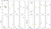 |
Fig. 5 Best-fit slab model parameters for the average VLMS spectrum (left circles) and T Tauri spectrum (right squares) for the different molecules. The H2O component for the T Tauri spectrum is the intermediate (T ~ 600) component. Temperature and column density are shown at the top on the left and right, respectively. The equivalent emitting radius is shown in the bottom left corner, and this radius normalized to the H2O snowline for each subsample is shown in the bottom right corner. Only the optically thick C2H2 component is shown for the VLMS in the radii plots because the radius is unconstrained in the optically thin case. The error bars were determined from the 1σ confidence intervals and in some cases are degenerate between parameters. For example, in the case of optically thin emission, the column density and equivalent emitting radii are degenerate. See Figures B.1 and B.2 for the χ2 maps for the T Tauri and VLMS fits, respectively. |
4 Discussion
We found a strong anticorrelation between the flux ratio of C2H2 to H2O and the stellar luminosity. Most of the targets fall within the  ratio found from the T Tauri modeling work of Anderson et al. (2021) (see their Figure 11, although we note that we did not use the same wavelength range to determine the fluxes). T Tauri objects with an observed
  would be most consistent with an oxygen-rich volatile content and a C/O ratio lower than 0.57, based on the models by Anderson et al. (2021). On the other hand, objects with host masses lower than ~0.2 M⊙ have significantly higher
  ratios than their higher-mass counterparts, which stems from their decreased H2O fluxes and increased C2H2 fluxes. This work builds upon trends seen with Spitzer observations by Pascucci et al. (2013) and initial results with JWST (see, e.g., Kamp et al. 2023; Long et al. 2025; Arabhavi et al. 2025a).
Many factors can affect the composition of disks and how much of the composition can be observed. Additionally, many of these factors can be related, which means that it the driver of the observed correlations in these samples is hard to determine. With this in mind, we explored the correlations we found and discuss the physical processes that might dominate the large difference in chemical signatures between VLMS and T Tauris stars.
4.1 Carbon enrichment or oxygen depletion in the VLMS disks
The hydrocarbon-dominated average VLMS spectrum in Figure 4 highlights the rich carbon chemistry that has been found in other VLMS with JWST thus far (e.g., Tabone et al. 2023; Arabhavi et al. 2024; Kanwar et al. 2024; Long et al. 2025; Morales-Calderón et al. 2025). Long et al. (2025) used the models of Najita et al. (2011), paired with the column density ratio of C2H2 to CO2, to determine the C/O ratio in their carbon-rich disk. We repeated this for the average fit spectra and found that the average VLMS has a C/O of ~1. It is worth investigating whether the high C/O ratio inferred for these disks is due to carbon enhancement and/or oxygen depletion.
The high derived C2H2 column densities (e.g., Tabone et al. 2023 and upper right panel of Figure 5) and the C2H2/HCN findings of Pascucci et al. (2009) indicate carbon enhancement in the VLMS disks. Additionally, the large hydrocarbon chains that include C2H6, C3H4, C4H2, and C6H6 indicate very abundant gas-phase carbon and a gas-phase C/O>1. We note that C2H4 and C2H6 are present in a few sources, but at shorter wave-lengths than we analyzed here (see Arabhavi et al. (2025a) for more details).
An interesting finding that discredits at least some oxygen depletion as the cause of the high C/O is the common presence of CO2 and 13CO2 in these disks (e.g., Tabone et al. 2023; Arabhavi et al. 2024, 2025a). Additionally, it has now been found that H2O is in fact present in these disks, albeit at very low flux levels (Arabhavi et al. 2025b). This agrees with the decrease in stellar luminosity (Figure A.1) and therefore emitting area, especially because the H2O snowline is very close to the central object in these disks. This will particularly affect the hottest H2O, mostly in the ro-vibrational lines at shorter wavelengths because the emitting area is very radially compact (see Figure 9 in Arabhavi et al. 2025b for a schematic). Another key oxygen tracer is CO because it locks up the bulk of the free oxygen when C/O>1. Interestingly, CO, at least the high Eup lines of the P-branch that is covered by MIRI MRS, is not frequently detected in disks around VLMSs: CO is in emission for only two of the ten VLMS sources in the MINDS program (Arabhavi et al. 2025a). It is unclear why oxygen is present in CO2 but only weakly in H2O or CO in these disks. Perhaps H2O and CO are present, but not readily observable, either due to the relative strength of the hydrocarbon Q-branches relative to the H2O lines and/or due to photospheric absorption that complicates the detection of disk CO emission (see Arabhavi et al. 2025a).
4.2 Stellar luminosity and the radiation field
The stellar luminosity is the main heating source for protoplanetary disks. This energy input drives the chemical evolution and equilibrium in the disks. The much lower luminosities of low-mass stars and brown dwarfs (L*~0.015 to 0.1 L⊙ for the sample we explored here) mean that their disks are much colder and the snowlines are much closer to the central hosts. The flux of the H2O lines follows the stellar luminosity and likely largely traces a change in emitting area (Salyk et al. 2011 and Figure A.1). On the other hand, the C2H2 flux does not follow this trend to the very low-mass parameter space, which indicates that the C2H2 flux is driven by something else besides the emitting area (see Appendix D in Arabhavi et al. 2025b for further discussion).
Young low-mass stars and brown dwarfs have different UV radiation spectra than Sun-like stars. Young M dwarfs are also known to be very active, however, and X-rays and extreme-UV from flares can affect the chemical evolution significantly (Feinstein et al. 2020). All of these differences in the radiation that impinges on the protoplanetary disk will affect the disk chemistry. The 2D thermochemical modeling by Walsh et al. (2015) showed that disks around M dwarfs are more molecule rich than their higher-mass counterparts. This is due at least in part to the weaker far-UV radiation for these low-mass stars. Similarly, the models of Woitke et al. (2024) showed that UV fluxes correlate with the line luminosities of OH and H2O, but the correlation with C2H2 and HCN is negative due to photodis-sociation. The two modeling works reported that X-ray-induced chemistry is important in setting the molecular complexity, in particular, for C2H2 and HCN, via the destruction of CO, N2, and H2. Therefore, the strong C2H2 emission in the VLMS disks may at least partially be caused by the weak UV fields of low-mass stars, paired with their still moderate X-ray fluxes. Sellek & van Dishoeck (2025) explored the effect of ionization on the disk chemistry, in particular, the destruction of CO by He+, and reported that the C that is liberated from CO can then go into the formation of hydrocarbons. This destruction pathway, paired with rapid radial transport, can result in high C/O in the inner disks of VLMSs at relatively young ages. For this scenario to work, relatively high ionization rates are needed for the VLMSs, which might be due to weaker shielding of the disks from cosmic rays by the stellar magnetic fields and/or to higher ionization from the central stars.
The UV emission that is generated by accretion of material from the disk onto the star will also be different between the T Tauris and VLMS stars. While the accretion mechanism is likely the same (i.e., magnetospheric accretion), the absolute accretion rate will decrease with decreasing stellar mass, and it might decrease even more rapidly below M*,<0.3 M⊙ (Manara et al. 2017). Colmenares et al. (2024) argued that the carbon-rich disk around a solar-type star they studied might be due to a combination of carbon grain destruction and an unusually low accretion rate that allows the carbon-rich gas to persist in the disk. As we showed in Figure 3,  and the accretion rate onto the star are related in our sample. While the degeneracies between the stellar mass and accretion rate make it difficult to determine what truly drives the correlation, however, we found that while
  decreases with decreasing accretion rate, the relation between accretion rate and
  is weaker (see Appendix A, Figure A.2). The low accretion rate of very low-mass objects might therefore contribute to the high observed
  in two ways: by keeping the H2O emitting area very small, and by not removing all of the carbon-rich gas quickly. We note, however, that stars with a mass lower than 0.3 M⊙ have been found to have a steeper Lacc/L* relation than higher-mass sources, which may come from their initially faster evolution (Manara et al. 2017). Thus, oxygen-rich gas may have been accreted fast at earlier ages, and carbon-rich gas accretes slowly by the age we observe these objects (see discussion in 4.3.2).
4.3 Dust evolution
4.3.1 Vertical dust settling
Dust is the main opacity source in protoplanetary disks. At the earliest stages, the submicron-sized particles are held aloft in the disk atmosphere, but these grains eventually grow from submicron particles into millimeter-sized grains to pebbles, protoplanets, and the cores of giant planets.
Spitzer-IRS observations provided unique insights into the compositions and properties of dust in the inner disk for systems with a wide diversity of properties, including central hosts from the brown dwarf to Herbig Ae/Be regime. These works found that disks around low-mass stars and brown dwarfs show 10 µm silicate emission features, which trace micron-sized dust grains in the disk atmosphere that are weaker than their more massive counterparts and features that show fairly high levels of crystallinity (Apai et al. 2005; Kessler-Silacci et al. 2007; Pascucci et al. 2009). This was now also found for objects with JWST (Kanwar et al. 2024; Kaeufer et al. 2024b). The radial location in the disk from which the 10 µm feature emits depends on the stellar luminosity, however, such that the emitting radius for brown dwarfs is much closer to the central object than for Herbig Ae/Be stars (≤0.001−0.1 au versus ≥0.5−50 au; Kessler-Silacci et al. 2007). Therefore, changes in the vertical dust scale, structure, or grain size distribution might therefore just reflect differences in the probed emitting region and not differences caused by the stellar influence or disk evolution. The 10 µm silicate features are generally weaker in disks around VLMS, and their strength might even be overestimated in some cases. Recent JWST observations have shown that broad features from 8.5 to 12.5 µm can in fact come at least partially from the high column densities of C2H4 (Arabhavi et al. 2024), which means that some of the already weak silicate features seen in low-mass objects with Spitzer might not even be due to dust emission. When they are present, however, the VLMS dust features in our sample are similar in strength to those in T Tauri systems with weak features. This supports the hypothesis that we see deeper into these disks. Further investigation of the dust properties in our VLMS sample will be included in separate work (Jang et al. 2025).
If the disks around low-mass hosts have undergone more efficient dust settling, this lack of small dust grains in the disk atmosphere means that these disks are subject to more stellar irradiation than those around their higher-mass counterparts, where the disk atmospheres are still relatively dust rich. This might lead to additional chemical reactions. The strongest implication of dust settling in low-mass sources is that mid-infrared observations probe more gas before it hits the τMIR=1 surface, however. This means that we are able to observe deeper into the disk than would otherwise be the case (see, e.g., the case of J160532, Tabone et al. 2023; Franceschi et al. 2024, and the modeling work of Greenwood et al. 2019; Antonellini et al. 2023; Houge et al. 2025b). We might thus be witnessing chemistry that may even be common in higher-mass systems, but is usually hidden from view. If this is the case, the optically thinner disks around low-mass sources may offer us a clearer picture of the midplane chemistry, where planet formation may be taking place. 2D thermochemical models found that the mid-infrared C2H2 emitting region is located deeper in the disk than H2O (e.g., Woitke et al. 2018). Paired with the high columns of carbon-rich gas we observe, this supports the idea that we probe closer to the disk midplane in disks around lower-mass objects (see Figure 9 in Arabhavi et al. 2025a for a schematic).
4.3.2 Radial dust drift
The inward drift of dust grains from the outer to the inner disk affects the chemical composition in the inner disk. These dust grains begin their journey in the cold outer disk, coated in various molecular ices. As they travel inward, they pass snowlines of different molecular species, which liberates their icy mantles as they pass and enriches the gas along the way. This drift can then supply the inner disk with, for instance, an increase in H2O vapor (Banzatti et al. 2020; Kalyaan et al. 2021; Banzatti et al. 2023). This drift will also increase the amount of dust in the inner disk, however, which can also shield the inner disk gas (e.g., Sellek et al. 2025; Houge et al. 2025b). Banzatti et al. (2020) found an anti-correlation between  and Rdust (in our formulation with C2H2 in the numerator, this would be a positive correlation: smaller disks have less C2H2 than H2O). In their sample of T Tauri stars, this indicated that dust drift might be shrinking the dust disks and enriching the inner regions in H2O. Conversely, if this drift is halted through a gap opening by a giant planet, for example, this can result in a relatively dry inner disk that lacks this additional oxygen enrichment (Najita et al. 2013).
Based on this expectation that drift-dominated disks are enriched in H2O vapor, we might expect that disks around VLMS are rich in H2O because their dust drift is efficient (e.g., Pinilla et al. 2013; Pinilla 2022). Mah et al. (2023) used disk evolution models to investigate this hypothesis and concluded that this enrichment might be so efficient and so rapid in low-mass systems that this occurs very early in the disk lifetime. If this oxygen-enriched gas were to then accrete onto the central star/brown dwarf, in particular, if accretion evolution occurs faster in these sources (Manara et al. 2017), this would leave only carbon-rich gas to advect inward later and more slowly from the outer disk (e.g., Miotello et al. 2019; Bosman et al. 2021). This might result in a time-dependent change in the disk C/O ratio, where C/O in disks around low-mass hosts decreases rapidly, followed by a gradual increase (see also Sellek et al. 2025). This might also explain the 30 Myr evolved carbon-rich disk analyzed by Long et al. (2025). The modeling work of Sellek & van Dishoeck (2025) showed that disks that are initially compact, as might generally be the case for disks around VLMSs, high C/O in the inner disk can be reached at young ages. If sub-structures were simply to slow down but not halt radial drift, however, this might prolong H2O enrichment (e.g., Kalyaan et al. 2023; Mah et al. 2024), which is the proposed explanation for the H2O-rich spectrum of a disk around a VLMS analyzed by Xie et al. (2023). Although we cannot explore any correlations with dust radius for the VLMS sample because only a few observations with a high angular resolution are available for these sources in general and in our sample particularly, we explored the relation between  and the disk dust mass (Figure 3). As with the accretion rate, the trend here might be driven by the correlation between M*, and Mdisk (Pascucci et al. 2016), and therefore, by the correlation with the stellar luminosity. The disk mass might in fact be a driving factor in setting the inner disk chemistry, however. More massive disks, which exist around more massive stars, will be able to form giant planets that are capable of forming traps that will halt radial drift (e.g., van der Marel & Mulders 2021). The low-mass disks around low-mass stars, on the other hand, might be (generally) incapable of forming these deep substructures, which would allow radial drift to occur efficiently and bring in ice-rich material quickly.
In order to observationally test the predicted connection between the drift and the inner disk chemistry in disks around very low-mass hosts, two steps are paramount: 1) Observations of disks around VLMSs at very young ages (≲0.5 Myr) to determine whether the gas is oxygen rich, and 2) high-resolution observations with ALMA to determine the outer radii and overall dust structure in disks around low-mass stars and brown dwarfs. The first can be accomplished with JWST observations of younger star-forming regions, and this is currently being investigated (e.g., PID 3886, PI: S. Grant), although observations of even younger sources (i.e., embedded Class I sources) might be required (e.g., PID 7890, PI: L. Tychoniec and PID 7135, PI: K. Zhang). The second step, that is, the connection between outer disk substructures and inner disk chemistry in VLMS disks, is challenging because the disks around very low-mass stars and brown dwarfs are faint. ALMA observations have only been made for a handful of sources at a high enough angular resolution and sensitivity in the gas and dust to determine the Rgas/Rdust ratio, which is expected to be high in the case of drift-dominated disks (Trapman et al. 2019; Toci et al. 2021). In shallow surveys, these disks are often undetected, let alone resolved spatially. Based on the small sample of resolved sources, however, drift indeed appears to be quite efficient in disks around these objects (Kurtovic et al. 2021). The overlap between the samples with JWST data and the high-resolution ALMA data is too small, however to characterize the outer disks in these exceptionally faint objects. Efforts to correct this lacking overlap are crucial to link the processes in outer disks to the chemistry in the inner disk in these systems (Xie et al. 2023). Some programs to do this are underway (e.g., 2024.1.00361.S, PI: F. Long). Finally, while the focus of our discussion here was on the early increase in C/O in low-mass systems, it should be noted that this scenario indicates that disks around T Tauri stars are expected to show an increase in C/O at later times. Therefore, the chemistry in the inner disk in T Tauri systems should be investigated across a range of ages to determine whether this an increase in the C/O ratio is seen on the timescales that are indicated by the models.
4.3.3 Carbon-grain destruction
Carbon-grain destruction is another viable method of increasing the gaseous C/O ratio in the inner disk (see the recent work of Houge et al. 2025a). While the sublimation temperature of refractory carbon species is debated in the literature, some estimates place the temperature as low as ~500 K (Li et al. 2021). If this so-called soot line were present in the disks around low-mass stars, the increase in gaseous carbon would allow for the formation of the carbon-rich gas species that are now observed (Tabone et al. 2023; Arabhavi et al. 2024). While the average fit parameters of the hydrocarbons in the VLMSs indicate low temperatures (the temperatures of CO2, HC3N, and C6H6 are all lower than 250 K), which might mean that this mechanism is not the dominant factor in enhancing the carbon in these disks. The grains might instead not be entirely destroyed and might simply be eroded by high-energy radiation or H atoms. If destruction/erosion like this occurs in these disks, the same effects might not be observed in most T Tauri disks because the higher dust opacities block the C-rich gas from being observed, and/or because the level of X-ray/cosmic-ray ionization is different. While this might be generally true, the carbon-rich spectrum of DoAr 33 has been analyzed in this context by Colmenares et al. (2024), who suggested that the low accretion rate of this object might allow the carbon-rich material to burn and linger. This might also explain our VLMS sources, which have low accretion rates. We note, however, that the correlation with the accretion rate (Figure 3) is weaker than the correlation with stellar luminosity (see also Figure A.2).
5 Summary and conclusions
We explored the transition from H2O-rich spectra to C2H2-dominated spectra with decreasing stellar luminosity using JWST-MIRI MRS observations from the MINDS collaboration that span (sub-)stellar masses from 0.02 to 1.5 M⊙. We list our results below.
The flux of H2O drops with decreasing stellar luminosity and accretion rate, as expected. Conversely, the C2H2 flux increases at the lowest host masses with an increase in the line-to-continuum ratio with decreasing L*. This is driven by the strong C2H2 features in the disks around low-mass stars and brown dwarfs.
We found a strong anticorrelation between
 and stellar luminosity. An anticorrelations also exist between this flux ratio and the strength of the 10 µm silicate feature, the accretion rate, and the disk mass. This might all be due in part to strong correlations with the stellar mass and luminosity, but it might be related to disk evolution processes that result in the abundant observed carbon-bearing species.
We computed the average spectra for the very low-mass sample (VLMS, M* ≤ 0.2 M⊙) and the T Tauri sample (M*, >0.2 M⊙). The average T Tauri spectrum is dominated by the forest of H2O lines, but features from C2H2, HCN, CO2, and OH are present. The average VLMS spectrum is dominated by the strong C2H2 Q-branch, with a molecular pseudo-continuum, with features from 13CCH2, HCN, C6H6, CO2, HC3N, C3H4, C4H2, CH3, and finally, weak H2O lines.
We used slab models to fit the average spectra for the T Tauri sample and the VLMS sample. We found that one component of the H2O emission in the T Tauri average has similar properties as the H2O in the average VLMS spectrum, although the VLMS H2O has a smaller emitting area, albeit in the optically thin regime, where the column density and emitting area are degenerate. One optically thick and one optically thin component are needed to reproduce the C2H2 emission in the VLMS spectrum, similar to what was found in individual VLMS spectra analyzed thus far. The hydrocarbon gas is generally quite cold, and the temperatures of CH3, HC3N, C3H4, C4H2 and C6H6 are lower than ~300 K.
We suggest that the
 correlation is driven by an increase in the volatile C/O ratio in the disks around very low-mass stars and brown dwarfs. More modeling work is needed to explore exactly how
  and C/O are connected, however, especially in low-mass systems, and extended carbon chemistry networks are required. If the high
  ratios for VLMS are due to a high gas phase C/O in the inner disk, this is likely driven by an enhancement in carbon-rich gas, rather than oxygen depletion alone. This carbon enrichment might be caused by the weaker UV radiation and/or X-ray/cosmic-ray ionization from very low-mass objects or by the different evolutionary timescales of their disks, in particular, the fast dust evolution that takes place in disks around VLMS, or some combination of multiple processes acting in concert. The latter can alter the chemistry via radial drift and/or by vertical dust settling. Vertical dust settling allows stellar radiation to penetrate closer to the disk midplane and means that our infrared observations probe deeper into the disk because the opacity is lower. Some of these potential processes are tightly linked to the age of the systems, which necessitates further exploration across a range of ages and evolutionary states in both stellar mass regimes.
By analyzing large samples of disks with a wide range of parameter space, we were able to investigate trends with system properties. Because many physical and chemical processes are correlated and in some cases, interconnected, however, it is crucial to scrutinize the samples over multiple axes to collect complementary data and to compare the observations to models in order to determine the driving processes.
Data availability
These observations are associated with program #1282 and can be accessed via DOI: https://archive.stsci.edu/doi/resolve/resolve.html?doi=10.17909/jeat-c950.
Acknowledgements
We thank the referee for constructive comments that improved the manuscript. This work is based on observations made with the NASA/ESA/CSA James Webb Space Telescope. The data were obtained from the Mikulski Archive for Space Telescopes at the Space Telescope Science Institute, which is operated by the Association of Universities for Research in Astronomy, Inc., under NASA contract NAS 5-03127 for JWST. The following National and International Funding Agencies funded and supported the MIRI development: NASA; ESA; Belgian Science Policy Office (BELSPO); Centre Nationale d'Etudes Spatiales (CNES); Danish National Space Centre; Deutsches Zentrum fur Luft- und Raumfahrt (DLR); Enterprise Ireland; Ministerio De Economía y Competividad; Netherlands Research School for Astronomy (NOVA); Netherlands Organisation for Scientific Research (NWO); Science and Technology Facilities Council; Swiss Space Office; Swedish National Space Agency; and UK Space Agency. E.v.D. acknowledges support from the ERC grant 101019751 MOLDISK and the Danish National Research Foundation through the Center of Excellence “InterCat” (DNRF150). M.T. and M.V. acknowledge support from the ERC grant 101019751 MOLDISK. A.M.A., I.K., and E.v.D. acknowledge support from grant TOP-1614.001.751 from the Dutch Research Council (NWO). B.T. is a Laureate of the Paris Region fellowship program (which is supported by the Ile-de-France Region) and has received funding under the Marie Sklodowska-Curie grant agreement No. 945298. T.H. and K.S. acknowledge support from the ERC Advanced Grant Origins 83 24 28. I.K. acknowledges funding from H2020-MSCA-ITN-2019, grant no. 860470 (CHAMELEON). A.C.G. has been supported by PRIN-INAF MAIN-STREAM 2017 and from PRIN-INAF 2019 (STRADE). V.C. acknowledges funding from the Belgian F.R.S.-FNRS. D.G. would like to thank the Research Foundation Flanders for co-financing the present research (grant number V435622N) and the European Space Agency (ESA) and the Belgian Federal Science Policy Office (BELSPO) for their support in the framework of the PRODEX Programme. T.K. acknowledges support from STFC Grant ST/Y002415/1. N.K. thanks the Deutsche Forschungsgemeinschaft (DFG) - grant 138 325594231, FOR 2634/2. M.M.C. has been funded by Spanish MCIN/AEI/10.13039/501100011033 grants PID2019-107061GB-C61 and No. MDM-2017-0737. G.P. gratefully acknowledges support from the Max Planck Society. L.M.S. has received funding from the European Research Council (ERC) under the European Union’s Horizon 2020 research and innovation programme (PROTOPLANETS, grant agreement No. 101002188).
References
- Alcalá, J. M., Manara, C. F., Natta, A., et al. 2017, A&A, 600, A20 [NASA ADS] [CrossRef] [EDP Sciences] [Google Scholar]
- Anderson, D. E., Blake, G. A., Cleeves, L. I., et al. 2021, ApJ, 909, 55 [NASA ADS] [CrossRef] [Google Scholar]
- Andrews, S. M., Rosenfeld, K. A., Kraus, A. L., & Wilner, D. J. 2013, ApJ, 771, 129 [Google Scholar]
- Antonellini, S., Kamp, I., & Waters, L. B. F. M. 2023, A&A, 672, A92 [NASA ADS] [CrossRef] [EDP Sciences] [Google Scholar]
- Apai, D., Pascucci, I., Bouwman, J., et al. 2005, Science, 310, 834 [NASA ADS] [CrossRef] [Google Scholar]
- Arabhavi, A. M., Kamp, I., Henning, T., et al. 2024, Science, 384, 1086 [NASA ADS] [CrossRef] [Google Scholar]
- Arabhavi, A. M., Kamp, I., Henning, T., et al. 2025a, A&A, 699, A194 [NASA ADS] [CrossRef] [EDP Sciences] [Google Scholar]
- Arabhavi, A. M., Kamp, I., van Dishoeck, E. F., et al. 2025b, ApJ, 984, L62 [Google Scholar]
- Arulanantham, N., Salyk, C., Pontoppidan, K., et al. 2025, AJ, 170, 67 [Google Scholar]
- Banzatti, A., Pascucci, I., Bosman, A. D., et al. 2020, ApJ, 903, 124 [NASA ADS] [CrossRef] [Google Scholar]
- Banzatti, A., Pontoppidan, K. M., Carr, J. S., et al. 2023, ApJ, 957, L22 [NASA ADS] [CrossRef] [Google Scholar]
- Banzatti, A., Salyk, C., Pontoppidan, K. M., et al. 2025, AJ, 169, 165 [Google Scholar]
- Bosman, A. D., Alarcón, F., Bergin, E. A., et al. 2021, ApJS, 257, 7 [NASA ADS] [CrossRef] [Google Scholar]
- Brown-Sevilla, S. B., Keppler, M., Barraza-Alfaro, M., et al. 2021, A&A, 654, A35 [NASA ADS] [CrossRef] [EDP Sciences] [Google Scholar]
- Bushouse, H., Eisenhamer, J., Dencheva, N., et al. 2024, JWST Calibration Pipeline (USA: NASA) [Google Scholar]
- Carnall, A. C. 2017, arXiv e-prints [arXiv:1705.05165] [Google Scholar]
- Colmenares, M. J., Bergin, E. A., Salyk, C., et al. 2024, ApJ, 977, 173 [NASA ADS] [CrossRef] [Google Scholar]
- Das, S., Kurtovic, N. T., & Flock, M. 2024, A&A, 689, A104 [NASA ADS] [CrossRef] [EDP Sciences] [Google Scholar]
- Erb, D. 2022, https://doi.org/10.5281/zenodo.7255880 [Google Scholar]
- Facchini, S., Teague, R., Bae, J., et al. 2021, AJ, 162, 99 [NASA ADS] [CrossRef] [Google Scholar]
- Fang, M., Pascucci, I., Edwards, S., et al. 2023, ApJ, 945, 112 [NASA ADS] [CrossRef] [Google Scholar]
- Feinstein, A. D., Montet, B. T., Ansdell, M., et al. 2020, AJ, 160, 219 [Google Scholar]
- Franceschi, R., Henning, T., Tabone, B., et al. 2024, A&A, 687, A96 [NASA ADS] [CrossRef] [EDP Sciences] [Google Scholar]
- Gangi, M., Antoniucci, S., Biazzo, K., et al. 2022, A&A, 667, A124 [NASA ADS] [CrossRef] [EDP Sciences] [Google Scholar]
- Gasman, D., van Dishoeck, E. F., Grant, S. L., et al. 2023, A&A, 679, A117 [NASA ADS] [CrossRef] [EDP Sciences] [Google Scholar]
- Grant, S. L., Espaillat, C. C., Brittain, S., Scott-Joseph, C., & Calvet, N. 2022, ApJ, 926, 229 [NASA ADS] [CrossRef] [Google Scholar]
- Grant, S. L., van Dishoeck, E. F., Tabone, B., et al. 2023, ApJ, 947, L6 [NASA ADS] [CrossRef] [Google Scholar]
- Grant, S. L., Kurtovic, N. T., van Dishoeck, E. F., et al. 2024, A&A, 689, A85 [NASA ADS] [CrossRef] [EDP Sciences] [Google Scholar]
- Greenwood, A. J., Kamp, I., Waters, L. B. F. M., Woitke, P., & Thi, W. F. 2019, A&A, 626, A6 [NASA ADS] [CrossRef] [EDP Sciences] [Google Scholar]
- Haffert, S. Y., Bohn, A. J., de Boer, J., et al. 2019, Nat. Astron., 3, 749 [Google Scholar]
- Hartmann, L., Herczeg, G., & Calvet, N. 2016, ARA&A, 54, 135 [Google Scholar]
- Henning, T., Kamp, I., Samland, M., et al. 2024, PASP, 136, 054302 [NASA ADS] [CrossRef] [Google Scholar]
- Herczeg, G. J., & Hillenbrand, L. A. 2014, ApJ, 786, 97 [Google Scholar]
- Hillenbrand, L. A., Strom, S. E., Vrba, F. J., & Keene, J. 1992, ApJ, 397, 613 [CrossRef] [Google Scholar]
- Houge, A., Johansen, A., Bergin, E., et al. 2025a, A&A, 699, A227 [NASA ADS] [CrossRef] [EDP Sciences] [Google Scholar]
- Houge, A., Krijt, S., Banzatti, A., et al. 2025b, MNRAS, 537, 691 [CrossRef] [Google Scholar]
- Jang, H., Arabhavi, A. M., Kaeufer, T., et al. 2025, A&A, in press, https://doi.org/10.1051/0004-6361/202556193 [Google Scholar]
- Kaeufer, T., Min, M., Woitke, P., Kamp, I., & Arabhavi, A. M. 2024a, A&A, 687, A209 [NASA ADS] [CrossRef] [EDP Sciences] [Google Scholar]
- Kaeufer, T., Woitke, P., Kamp, I., Kanwar, J., & Min, M. 2024b, A&A, 690, A100 [NASA ADS] [CrossRef] [EDP Sciences] [Google Scholar]
- Kalyaan, A., Pinilla, P., Krijt, S., Mulders, G. D., & Banzatti, A. 2021, ApJ, 921, 84 [CrossRef] [Google Scholar]
- Kalyaan, A., Pinilla, P., Krijt, S., et al. 2023, ApJ, 954, 66 [NASA ADS] [CrossRef] [Google Scholar]
- Kamp, I., Henning, T., Arabhavi, A. M., et al. 2023, Faraday Discuss., 245, 112 [NASA ADS] [CrossRef] [Google Scholar]
- Kanwar, J., Kamp, I., Jang, H., et al. 2024, A&A, 689, A231 [NASA ADS] [CrossRef] [EDP Sciences] [Google Scholar]
- Kessler-Silacci, J., Augereau, J.-C., Dullemond, C. P., et al. 2006, ApJ, 639, 275 [NASA ADS] [CrossRef] [Google Scholar]
- Kessler-Silacci, J. E., Dullemond, C. P., Augereau, J. C., et al. 2007, ApJ, 659, 680 [NASA ADS] [CrossRef] [Google Scholar]
- Kurtovic, N. T., Pinilla, P., Long, F., et al. 2021, A&A, 645, A139 [EDP Sciences] [Google Scholar]
- Li, J., Bergin, E. A., Blake, G. A., Ciesla, F. J., & Hirschmann, M. M. 2021, Sci. Adv., 7, eabd3632 [NASA ADS] [CrossRef] [Google Scholar]
- Long, F., Pascucci, I., Houge, A., et al. 2025, ApJ, 978, L30 [Google Scholar]
- Luhman, K. L. 2007, ApJS, 173, 104 [Google Scholar]
- Mah, J., Bitsch, B., Pascucci, I., & Henning, T. 2023, A&A, 677, L7 [CrossRef] [EDP Sciences] [Google Scholar]
- Mah, J., Savvidou, S., & Bitsch, B. 2024, A&A, 686, L17 [NASA ADS] [CrossRef] [EDP Sciences] [Google Scholar]
- Manara, C. F., Rosotti, G., Testi, L., et al. 2016, A&A, 591, L3 [NASA ADS] [CrossRef] [EDP Sciences] [Google Scholar]
- Manara, C. F., Testi, L., Herczeg, G. J., et al. 2017, A&A, 604, A127 [NASA ADS] [CrossRef] [EDP Sciences] [Google Scholar]
- Manara, C. F., Ansdell, M., Rosotti, G. P., et al. 2023, ASP Conf. Ser., 534, 539 [NASA ADS] [Google Scholar]
- Manjavacas, E., Tremblin, P., Birkmann, S., et al. 2024, AJ, 167, 168 [NASA ADS] [CrossRef] [Google Scholar]
- Mendigutía, I., Oudmaijer, R. D., Rigliaco, E., et al. 2015, MNRAS, 452, 2837 [Google Scholar]
- Min, M., Dullemond, C. P., Kama, M., & Dominik, C. 2011, Icarus, 212, 416 [Google Scholar]
- Miotello, A., Facchini, S., van Dishoeck, E. F., et al. 2019, A&A, 631, A69 [NASA ADS] [CrossRef] [EDP Sciences] [Google Scholar]
- Morales-Calderón, M., Jang, H., Arabhavi, A. M., et al. 2025, in press, https://doi.org/10.1051/0004-6361/202555621 [Google Scholar]
- Muñoz-Romero, C. E., Öberg, K. I., Banzatti, A., et al. 2024, ApJ, 964, 36 [CrossRef] [Google Scholar]
- Mulders, G. D., Ciesla, F. J., Min, M., & Pascucci, I. 2015, ApJ, 807, 9 [NASA ADS] [CrossRef] [Google Scholar]
- Najita, J. R., Ádámkovics, M., & Glassgold, A. E. 2011, ApJ, 743, 147 [NASA ADS] [CrossRef] [Google Scholar]
- Najita, J. R., Carr, J. S., Pontoppidan, K. M., et al. 2013, ApJ, 766, 134 [Google Scholar]
- Öberg, K. I., & Bergin, E. A. 2021, Phys. Rep., 893, 1 [Google Scholar]
- Pascucci, I., Apai, D., Luhman, K., et al. 2009, ApJ, 696, 143 [Google Scholar]
- Pascucci, I., Herczeg, G., Carr, J. S., & Bruderer, S. 2013, ApJ, 779, 178 [NASA ADS] [CrossRef] [Google Scholar]
- Pascucci, I., Testi, L., Herczeg, G. J., et al. 2016, ApJ, 831, 125 [Google Scholar]
- Pascucci, I., Banzatti, A., Gorti, U., et al. 2020, ApJ, 903, 78 [Google Scholar]
- Patapis, P., Morales-Calderón, M., Arabhavi, A. M., et al. 2025, A&A, submitted [arXiv:2507.08961] [Google Scholar]
- Pecaut, M. J., & Mamajek, E. E. 2016, MNRAS, 461, 794 [Google Scholar]
- Perotti, G., Christiaens, V., Henning, T., et al. 2023, Nature, 620, 516 [NASA ADS] [CrossRef] [Google Scholar]
- Pinilla, P. 2022, Eur. Phys. J. Plus, 137, 1206 [NASA ADS] [CrossRef] [Google Scholar]
- Pinilla, P., Birnstiel, T., Benisty, M., et al. 2013, A&A, 554, A95 [NASA ADS] [CrossRef] [EDP Sciences] [Google Scholar]
- Pontoppidan, K. M., Salyk, C., Bergin, E. A., et al. 2014, in Protostars and Planets VI, eds. H. Beuther, R. S. Klessen, C. P. Dullemond, & T. Henning (Tucson: University of Arizona Press), 363 [Google Scholar]
- Pontoppidan, K. M., Salyk, C., Banzatti, A., et al. 2024, ApJ, 963, 158 [NASA ADS] [CrossRef] [Google Scholar]
- Romero-Mirza, C. E., Banzatti, A., Öberg, K. I., et al. 2024, ApJ, 975, 78 [NASA ADS] [CrossRef] [Google Scholar]
- Salyk, C., Pontoppidan, K. M., Blake, G. A., Najita, J. R., & Carr, J. S. 2011, ApJ, 731, 130 [Google Scholar]
- Salyk, C., Pontoppidan, K. M., Banzatti, A., et al. 2025, AJ, 169, 184 [Google Scholar]
- Sellek, A. D., & van Dishoeck, E. F. 2025, A&A, 701, A239 [NASA ADS] [CrossRef] [EDP Sciences] [Google Scholar]
- Sellek, A. D., Vlasblom, M., & van Dishoeck, E. F. 2025, A&A, 694, A79 [NASA ADS] [CrossRef] [EDP Sciences] [Google Scholar]
- Tabone, B., Bettoni, G., van Dishoeck, E. F., et al. 2023, Nat. Astron., 7, 805 [NASA ADS] [CrossRef] [Google Scholar]
- Temmink, M., van Dishoeck, E. F., Gasman, D., et al. 2024a, A&A, 689, A330 [NASA ADS] [CrossRef] [EDP Sciences] [Google Scholar]
- Temmink, M., van Dishoeck, E. F., Grant, S. L., et al. 2024b, A&A, 686, A117 [NASA ADS] [CrossRef] [EDP Sciences] [Google Scholar]
- Testi, L., Natta, A., Manara, C. F., et al. 2022, A&A, 663, A98 [NASA ADS] [CrossRef] [EDP Sciences] [Google Scholar]
- Toci, C., Rosotti, G., Lodato, G., Testi, L., & Trapman, L. 2021, MNRAS, 507, 818 [NASA ADS] [CrossRef] [Google Scholar]
- Trapman, L., Facchini, S., Hogerheijde, M. R., van Dishoeck, E. F., & Bruderer, S. 2019, A&A, 629, A79 [NASA ADS] [CrossRef] [EDP Sciences] [Google Scholar]
- van Boekel, R., Waters, L. B. F. M., Dominik, C., et al. 2003, A&A, 400, L21 [NASA ADS] [CrossRef] [EDP Sciences] [Google Scholar]
- van der Marel, N., & Mulders, G. D. 2021, AJ, 162, 28 [NASA ADS] [CrossRef] [Google Scholar]
- Vlasblom, M., Temmink, M., Grant, S. L., et al. 2025, A&A, 693, A278 [NASA ADS] [CrossRef] [EDP Sciences] [Google Scholar]
- Walsh, C., Nomura, H., & van Dishoeck, E. 2015, A&A, 582, A88 [NASA ADS] [CrossRef] [EDP Sciences] [Google Scholar]
- Wendeborn, J., Espaillat, C. C., Lopez, S., et al. 2024, ApJ, 970, 118 [Google Scholar]
- Woitke, P., Min, M., Thi, W. F., et al. 2018, A&A, 618, A57 [NASA ADS] [CrossRef] [EDP Sciences] [Google Scholar]
- Woitke, P., Thi, W. F., Arabhavi, A. M., et al. 2024, A&A, 683, A219 [NASA ADS] [CrossRef] [EDP Sciences] [Google Scholar]
- Wright, G. S., Rieke, G. H., Glasse, A., et al. 2023, PASP, 135, 048003 [NASA ADS] [CrossRef] [Google Scholar]
- Xie, C., Pascucci, I., Long, F., et al. 2023, ApJ, 959, L25 [NASA ADS] [CrossRef] [Google Scholar]
Appendix A  , and the line-to-continuum ratio
The relations between the absolute flux values of C2H2 and H2O and the line-to-continuum ratios for those molecules as a function of stellar luminosity are presented in Figure A.1. The  , relation is largely as expected: the lower luminosity of the host, the lower the line luminosity, although we may be limited by sensitivity for the H2O lines in the VLMS sample. By contrast, there is no clear
  . relation; however, there is a correlation between the line-to-continuum ratio for C2H2 and the stellar luminosity. The relations between the absolute fluxes and the strength of the 10 µm silicate feature, stellar accretion rate, and the disk dust mass are presented in Figure A.2. The strongest correlation there is between the H2O flux and the stellar accretion rate, found similarly between
  and the accretion luminosity by Banzatti et al. (2020). However, the trend between the C2H2 line flux and the accretion rate, while present, is not very strong. This may be due to the bright C2H2 fluxes of the VLMS, as correlations have been seen between C2H2 and Ṁ in T Tauri samples by Banzatti et al. (2020) and Arulanantham et al. (2025).
Woitke et al. (2024) find that the flux of C2H2 reacts more strongly to an increase in accretion rate than H2O does, which is not what we find in our sample. Given the relation between accretion rate and stellar luminosity (see e.g., Manara et al. 2023 and references therein), we also check  vs. Ṁ/M*, which are correlated, but with a weaker correlation than
  and than
  .
.
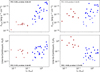 |
Fig. A.1 The absolute fluxes of H2O (top left) and C2H2 (top right) as a function of stellar luminosity. The fluxes are determined after normalizing the spectra to a distance of 120 pc. The line-to-continuum ratio for H2O and C2H2 as a function of stellar luminosity are shown in the bottom left and right, respectively. Upper limits (downward triangles) are the 3σ fluxes. Error bars are smaller than the points for most targets. The blue points are the T Tauri sample and the red points are the VLMS targets. The PCCs and p-values can be found for each panel. Significant correlations (p-value<0.05) are provided in bold. |

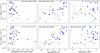 |
Fig. A.2 The absolute fluxes of C2H2 (top) and H2O (bottom) as a function of the strength of the 10 µm silicate feature (left), stellar accretion rate (middle), and dust disk mass (right). The fluxes are normalized to a distance of 120 pc. Upper limits (downward triangles) are the 3σ fluxes; objects with Mdust upper limits are either leftward facing triangles if the molecular species is detected, or rotated triangular markers if both the flux and dust mass are upper limits. Error bars are smaller than the points for most targets. The blue points are the T Tauri sample and the red points are the VLMS targets. The PCCs and p-values can be found for each panel. Significant correlations (p-value<0.05) are provided in bold. |
Appendix B χ2 maps
The reduced χ2 maps for the molecules detected in the average T Tauri and VLMS spectra are shown in Figures B.1 and B.2, respectively. The contours are the 1σ, 2σ, and 3σ levels determined as  ,
,  , and
, and  , respectively (see Appendix C of Grant et al. 2023 for details).
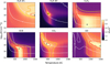 |
Fig. B.1 The χ2 maps for the molecules fitted in the average T Tauri spectrum. The color-scale shows |

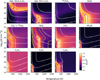 |
Fig. B.2 Same as Figure B.1, but now for the molecules in the average VLMS spectrum. |
All Tables
All Figures
|
Fig. 1 Average T Tauri (top) and VLMS (bottom) sample JWST spectra. The detected molecular species are highlighted. The C2H2 and H2O regions (yellow and blue, respectively) show the regions over which the fluxes were integrated. Most of the unlabeled lines in the T Tauri average are various H2O transitions. |
| In the text | |
|
Fig. 2 Relation between the flux ratio of C2H2 to H2O as a function of stellar luminosity. Objects with M*>0.2 M⊙ are shown in blue and represent our T Tauri sample, and those with stellar masses below 0.2 M⊙ are our VLMS sample and are shown in red. The two outliers around L* ~ 1 L⊙ are DL Tau and V1094 Sco, which will be analyzed in detail in Tabone et al. (in prep.). This trend is statistically significant with a p-value of 1.3×10⁻⁷ and a correlation coefficient of −0.77. 3σ upper and lower limits are the downward and upward triangles, respectively. The error bars are smaller than the points for most targets. |
| In the text | |
|
Fig. 3 Left: |
| In the text | |
|
Fig. 4 Average spectra for disks in our T Tauri sample (top) and VLMS sample (bottom) in black, compared to the best-fit model in red. The model components are shown below each for reference. |
| In the text | |
|
Fig. 5 Best-fit slab model parameters for the average VLMS spectrum (left circles) and T Tauri spectrum (right squares) for the different molecules. The H2O component for the T Tauri spectrum is the intermediate (T ~ 600) component. Temperature and column density are shown at the top on the left and right, respectively. The equivalent emitting radius is shown in the bottom left corner, and this radius normalized to the H2O snowline for each subsample is shown in the bottom right corner. Only the optically thick C2H2 component is shown for the VLMS in the radii plots because the radius is unconstrained in the optically thin case. The error bars were determined from the 1σ confidence intervals and in some cases are degenerate between parameters. For example, in the case of optically thin emission, the column density and equivalent emitting radii are degenerate. See Figures B.1 and B.2 for the χ2 maps for the T Tauri and VLMS fits, respectively. |
| In the text | |
|
Fig. A.1 The absolute fluxes of H2O (top left) and C2H2 (top right) as a function of stellar luminosity. The fluxes are determined after normalizing the spectra to a distance of 120 pc. The line-to-continuum ratio for H2O and C2H2 as a function of stellar luminosity are shown in the bottom left and right, respectively. Upper limits (downward triangles) are the 3σ fluxes. Error bars are smaller than the points for most targets. The blue points are the T Tauri sample and the red points are the VLMS targets. The PCCs and p-values can be found for each panel. Significant correlations (p-value<0.05) are provided in bold. |
| In the text | |
|
Fig. A.2 The absolute fluxes of C2H2 (top) and H2O (bottom) as a function of the strength of the 10 µm silicate feature (left), stellar accretion rate (middle), and dust disk mass (right). The fluxes are normalized to a distance of 120 pc. Upper limits (downward triangles) are the 3σ fluxes; objects with Mdust upper limits are either leftward facing triangles if the molecular species is detected, or rotated triangular markers if both the flux and dust mass are upper limits. Error bars are smaller than the points for most targets. The blue points are the T Tauri sample and the red points are the VLMS targets. The PCCs and p-values can be found for each panel. Significant correlations (p-value<0.05) are provided in bold. |
| In the text | |
|
Fig. B.1 The χ2 maps for the molecules fitted in the average T Tauri spectrum. The color-scale shows |
| In the text | |
|
Fig. B.2 Same as Figure B.1, but now for the molecules in the average VLMS spectrum. |
| In the text | |
Current usage metrics show cumulative count of Article Views (full-text article views including HTML views, PDF and ePub downloads, according to the available data) and Abstracts Views on Vision4Press platform.
Data correspond to usage on the plateform after 2015. The current usage metrics is available 48-96 hours after online publication and is updated daily on week days.
Initial download of the metrics may take a while.