| Issue |
A&A
Volume 702, October 2025
|
|
|---|---|---|
| Article Number | A223 | |
| Number of page(s) | 17 | |
| Section | Galactic structure, stellar clusters and populations | |
| DOI | https://doi.org/10.1051/0004-6361/202556039 | |
| Published online | 24 October 2025 | |
Dynamics of tidal spiral arms: Machine learning-assisted identification of equations and application to the Milky Way
1
Departament de Física Quàntica i Astrofísica (FQA), Universitat de Barcelona (UB),
c. Martí i Franquès, 1,
08028
Barcelona,
Spain
2
Institut de Ciències del Cosmos (ICCUB), Universitat de Barcelona (UB),
c. Martí i Franquès, 1,
08028
Barcelona,
Spain
3
Institut d’Estudis Espacials de Catalunya (IEEC), Edifici RDIT, Campus UPC,
08860
Castelldefels (Barcelona),
Spain
4
National Astronomical Observatory of Japan,
Mitaka-shi, Tokyo
181-8588,
Japan
5
Center for Computational Astrophysics, Flatiron Institute,
162 Fifth Ave,
New York,
NY
10010,
USA
6
Department of Mechanical Engineering, University of Washington,
Seattle,
Washington
98195,
USA
7
AI Institute in Dynamic Systems, University of Washington,
Seattle,
WA
98195,
USA
★ Corresponding author: This email address is being protected from spambots. You need JavaScript enabled to view it.
Received:
20
June
2025
Accepted:
21
August
2025
Abstract
Context. Understanding the spiral arms of the Milky Way (MW) remains a key open question in galactic dynamics. Tidal perturbations, such as the recent passage of the Sagittarius dwarf galaxy (Sgr), could play a significant role in exciting them.
Aims. We aim to analytically characterise the dynamics of tidally induced spiral arms, including their phase-space signatures.
Methods. We ran idealised test-particle simulations resembling impulsive satellite impacts and used the Sparse Identification of Non-linear Dynamics (SINDy) method to infer their governing partial differential equations (PDEs). We validated the method with analytical derivations and a realistic N-body simulation of a MW-Sgr encounter analogue.
Results. For small perturbations, a linear system of equations was recovered with SINDy, consistent with predictions from linearised collisionless dynamics. In this case, two distinct waves wrapping at pattern speeds Ω ± κ/m emerge, where Ω and κ are the azimuthal and epicyclic frequencies, and m is the azimuthal mode number. For large impacts, we empirically discovered a non-linear system of equations, representing a novel formulation for the dynamics of tidally induced spiral arms. For both cases, these equations describe wave properties like amplitude and pattern speed, along with their shape and temporal evolution in different phase-space projections. In the realistic simulations, we recovered the same equation. However, the fit is sub-optimal, pointing to missing terms in our analysis, such as velocity dispersion and self-gravity. We fit the Gaia LZ−〈VR〉 waves with the linear model, providing a reasonable fit and plausible parameters for the Sgr passage. However, the predicted amplitude ratio of the two waves is inconsistent with observations, supporting a more complex origin for this feature (e.g. multiple passages, bar, spiral arms).
Conclusions. We merged data-driven discovery with theory to create simple, accurate models of tidal spiral arms that match simulations and provide a simple tool to fit Gaia and external galaxy data. This methodology could be extended to model complex phenomena such as self-gravity and dynamical friction.
Key words: methods: data analysis / Galaxy: disk / Galaxy: evolution / Galaxy: kinematics and dynamics / Galaxy: structure
© The Authors 2025
 Open Access article, published by EDP Sciences, under the terms of the Creative Commons Attribution License (https://creativecommons.org/licenses/by/4.0), which permits unrestricted use, distribution, and reproduction in any medium, provided the original work is properly cited.
This article is published in open access under the Subscribe to Open model. This email address is being protected from spambots. You need JavaScript enabled to view it. to support open access publication.
1 Introduction
Understanding the dynamics of the spiral arms of the Milky Way (MW) remains a major challenge in galactic astronomy (Dobbs & Baba 2014; Sellwood & Masters 2022). Theoretical models range from density wave theories (Lin & Shu 1964; Kalnajs 1973), to transient and recurrent, swing-amplified instabilities (Goldreich & Lynden-Bell 1965; Julian & Toomre 1966), and self-excited spiral modes (Sellwood & Carlberg 1984), with varying consequences for the spiral pattern speed, pitch angle, and bar-spiral coupling (Lynden-Bell & Kalnajs 1972; Sanders & Huntley 1976; Sellwood & Masters 2022). In the MW, even though spiral arm segments can be traced by young stars and gas (Georgelin & Georgelin 1976; Drimmel & Spergel 2001; Reid et al. 2009), their number, longevity, and origin are still a matter of debate.
The Gaia mission (Gaia Collaboration 2016) has revealed complex kinematic substructures across various phase space projections, the R − Vϕ plane (e.g. Antoja et al. 2018; Kawata et al. 2018; Fragkoudi et al. 2019; Ramos et al. 2018; Bernet et al. 2024), wave-like patterns in R − VR and LZ − VR (e.g. Friske & Schönrich 2019; Eilers et al. 2020; Antoja et al. 2022; Hunt et al. 2024), thin arches in VR − Vϕ(e.g. Gaia Collaboration 2018; Bernet et al. 2022; Bernet et al. 2024), and a vertical phase spiral in Z − VZ (e.g. Antoja et al. 2018; Laporte et al. 2019; Bland-Hawthorn & Tepper-García 2021; Hunt et al. 2021; Antoja et al. 2023; Darragh-Ford et al. 2023). Interpreting the origin and evolution of these global disequilibrium features requires theoretical modelling procedures that account for the effects of the bar, spiral arms, and perturbations with external galaxies.
In Antoja et al. (2022, hereafter A22), we were motivated by the evidence of ongoing vertical phase mixing in the disc (Antoja et al. 2018). Assuming that it is likely due to the interaction with the Sagittarius (Sgr) dwarf galaxy (Ibata et al. 1994), we developed a framework to interpret some of the planar features observed in the MW disc in terms of tidally induced spiral arms. By combining analytical models with test particle simulations and an N-body model of the Sgr–MW interaction (Laporte et al. 2018), we showed how a tidal impact produces spiral arms that phase-wrap over time and are manifested as coherent ridges in R − Vϕand waves in Lz − VR. However, A22 was limited to deriving only the spiral arm loci over time, as the full dynamics captured in simulations can be remarkably challenging to model analytically.
While a deep foundation in theoretical and analytical models has historically shaped our understanding of galactic dynamics (e.g. Binney & Tremaine 2008), the explosion of high-precision data and modern simulations is transforming the field. This presents an opportunity for data-driven approaches, where we can use the data itself to empirically discover the underlying dynamical principles. Inferring physical laws from data is a long-standing practice in astronomy. Centuries ago, Kepler employed symbolic regression to derive his empirical laws of planetary motion (Kepler 1609). More recently, Tenachi et al. (2023, 2024) have introduced a general deep learning framework for extracting analytical governing laws from simulated and/or observed data, which they successfully applied to derive an analytic galaxy potential directly from simulated stellar orbits.
Beyond these examples in astronomy, significant advancements have been made in data-driven methods for discovering the governing equations of complex dynamical systems across various scientific domains. A pioneering approach is Sparse Identification of Nonlinear Dynamics (SINDy), introduced by Brunton et al. (2016), which uses sparse regression to identify the governing ordinary differential equations (ODEs) of a dynamical system directly from time-series data. This idea was subsequently extended to partial differential equations (PDEs) by Rudy et al. (2017) and Schaeffer (2017), utilising spatial-temporal data. Techniques such as the integral or weak formulation (Schaeffer & McCalla 2017; Reinbold et al. 2020) have further refined these methods, improving robustness to noise and handling high-order derivatives. These advances have enabled the data-driven discovery (or rediscovery) of governing PDEs in various physical domains, including geophysical fluids (Zanna & Bolton 2020), plasma physics (Alves & Fiuza 2022), active matter (Supekar et al. 2023), and turbulence closure modelling (Beetham & Capecelatro 2020; Schmelzer et al. 2020; Zanna & Bolton 2020; Beetham et al. 2021). A comprehensive review of these methods is provided by North et al. (2023). Other related techniques for discovering dynamical systems, particularly for ordinary differential equations, include symbolic regression through genetic programming (Bongard & Lipson 2007; Schmidt & Lipson 2009; Cranmer 2023).
In this work, we use a data-driven dynamical discovery approach to understand tidally induced spiral arm dynamics. We built idealised test-particle simulations (Sect. 2) and used SINDy to infer their governing equations (Sect. 3). This approach reveals two families of PDEs that govern spiral wave evolution. For small perturbations, we recovered a linear system of equations, consistent with predictions from established linearised collision-less theory. For large perturbations with specific profiles, SINDy empirically identified a non-linear system of equations. Notably, this PDE itself constitutes a novel mathematical formulation for the dynamics of tidally induced spiral arms. Guided by these empirical findings, we analytically derived these same equations from first principles (Sect. 4), recovering closed expressions for their coefficients and obtaining explicit solutions that describe wave properties like amplitude and pattern speed, and their shape and temporal evolution in different phase-space projections.
This framework is validated against realistic N-body simulations (Sect. 5). Finally, we use these analytical solutions to test whether our simple models can reproduce the characteristics of the LZ−〈VR〉 wave seen in the Gaia data (Sect. 6). Our work demonstrates how data-driven methods can lead to the discovery of simple governing equations that can be solved analytically and provide interpretable, predictive models for key kinematic features observed in the MW and other galaxies perturbed by internal or external forces.
2 Test particle simulations for tidal impacts
This section describes our 2D test-particle simulations. We run them with Agama (Vasiliev 2019). We used the classical MWPotential2014 (Bovy 2015), consisting of a Miyamoto & Nagai (1975) disk, a NFW (Navarro et al. 1996) halo and a Dehnen (1993) bulge. The dynamical features we study here are present in any reasonable axisymmetric potential (logarithmic, Plummer, etc.); thus, our results do not depend on this choice. We initialised all test particles on perfectly circular orbits, with zero velocity dispersion. Thus, each particle then satisfied
 (1)
(1)
where Vc is the circular velocity curve of the assumed model. We sampled 106 particles using a uniform distribution in R to increase the signal in the outer disc.
Once these initial conditions (ICs) were set up, we induced a perturbation to the system. In this section, we describe how we applied three types of perturbations to these ICs: a distant and small impact (Sect. 2.1), a generalised small impact (Sect. 2.2), and a large impact (Sect. 2.3). Each perturbation generates a distinctive kinematic signal that we aim to understand in this work.
2.1 Distant and small impacts
To simulate a weak and distant impulsive encounter, we employed the impulse approximation (the perturber passes quickly) and the tidal approximation (the perturber is distant). Under these strong assumptions, the complex, time-evolving gravitational interaction is simplified to a single, instantaneous velocity kick. For the purposes of this work, we did not model a specific encounter orbit; instead we adopted the following canonical form (e.g. Aguilar & White 1985; Struck et al. 2011), which matches, to first order, the kinematic response of realistic N-body models (A22):
 (2)
(2)
which are added to the ICs defined in Eq. (1). The direction of closest approach was arbitrarily chosen to be ϕ = 0 (equivalent to ϕ = π), resulting in the maximum kick in VR being at the same azimuth. The scale parameter ϵ, in units of km s−1 kpc−1, sets the amplitude of this initial velocity kick. For a quick flyby by a mass, Mp, at closest distance, rp, with a velocity, υp, ϵ, can be estimated as  (Sect. 8.2.1. in Binney & Tremaine 2008). In this section, we assume a small impact, which we define as a perturbation where the response of the system is linear. This requires the velocity kick to be much smaller than the circular velocity (∆VR, ∆Vϕ ≪Vc) and, therefore, a small ϵ. For this work, we quantitatively considered the small impact regime to correspond to kick amplitudes of ϵ ≲ 0.1 km s−1 kpc−1, which leads to a velocity kick of ≲ 10 km s−1 at the studied radii. The two-fold symmetry1 in the radial (∆VR) and azimuthal (∆Vϕ) velocity fields can be seen in the leftmost panels of the upper rows in Fig. 1.
After evolving these initial conditions for 0.4 Gyr, we found two distinct wave modes emerging in the velocity field. The primary wave is seen mostly in the wrapping of the velocity patterns in a spiral shape (red-blue) of large scale. This leads to a density enhancement in regions of negative VR that constitute the spiral arms (see Fig. 4 in A22). The secondary wave is fainter and wraps faster, so it is seen as smaller scale oscillations superimposed on of the main pattern. Further details and visualisations of the resulting 1D radial profiles, illustrating the contributions of the primary and secondary waves, are presented in Appendix A. We see that the pattern speed of the primary spiral wave is Ω − κ/2, which is widely known (e.g. Kalnajs 1973; Oh et al. 2008, 2015; Struck et al. 2011; Semczuk et al. 2017), although the presence of a bar or self-gravity can modify this pattern speed, up to Ω − κ/4 (e.g. Oh et al. 2015; Pettitt & Wadsley 2018). On the other hand, in A22, we already noted the presence of the secondary wave, although we did not characterise it. We see here that it wraps as Ω + κ/2. In Sect. 4, we give the analytical explanation for its appearance and its wrapping frequency.
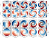 |
Fig. 1 Kinematic signature evolution of the m = 2 (upper panels) and m = 1 (lower panels) kinematic kicks. We show snapshots of the velocity perturbation fields at five different times (t = 0, 0.1, 0.2, 0.3, and 0.4 Gyr). For each kick mode, the top row displays the radial velocity perturbation, ∆VR, while the bottom row shows the azimuthal velocity perturbation, ∆Vϕ. The solid and dash-dotted curves overlaid on the ∆VR panels indicate the theoretical spiral loci wrapping at pattern speeds Ω − κ/m and Ω + κ/m, respectively. The panels demonstrate the clear appearance of two spiral wave patterns for both m = 2 and m = 1 modes, with the theoretical loci accurately matching the observed evolution of the waves in the velocity fields. |
2.2 Generalised kinematic kick
The framework assumes an m = 2 kinematic kick, but we can extend this formulation to include other perturbation shapes, accounting for more complex patterns with multiple m modes from more realistic galactic encounters and halo misalignments (e.g. Chakrabarti & Blitz 2009; Ghosh et al. 2022). Here, we apply idealised m-mode kinematic kicks as a controlled experiment to isolate the dynamical response to specific shapes of the ICs. Specifically, we can generalise Eq. (2) to
 (3)
(3)
In the bottom group of Fig. 1, we show the velocity maps for an m = 1 kick. In this case, the two waves wrap at frequencies of Ωsp = Ω ± κ. In general, for every m-shaped kick we include, two spiral patterns emerge, wrapping according to:
 (4)
(4)
The basic intuition is as follows: each star circles around its reference (guiding) orbit at an angular rate Ω and, in addition, executes small radial (epicyclic) oscillations at a frequency κ. A single star completes one full radial oscillation, reaching repeatedly its apocentre, at this epicyclic frequency κ. However, the imposed m-fold symmetry in the initial perturbation sets the number of apocentres in a given radius. Instead of observing one apocentre per full κ epicycle, the symmetry causes the collective apocentre pattern to repeat every κ/m. Therefore, between two consecutive apocentres of a single star, one observes additional apocentres from other stars – a total of m, spread evenly across the circle. This sets the precession rate, creating the pattern described in Eq. (4).
At a fixed radius, the amplitudes of the primary wave (Ω − κ/m) and the secondary wave (Ω + κ/m) remain constant in time and are independent of the azimuthal number m. Their relative strength, however, varies with radius and with the choice of gravitational potential. In our fiducial model we have measured the relative amplitude of both waves by computing the 2D Fourier amplitude in ϕ − t maps. The ratio of amplitudes between both waves stays nearly constant throughout the disk, taking a value very close to
 (5)
(5)
where 𝒜 represents the amplitude of a wave. In Section 4, we recover this value from first principles.
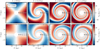 |
Fig. 2 Evolution of the test-particle system after a large, m = 2 impact, designed with a γ correction (Eq. (6)) to excite a single spiral pattern. These panels show snapshots of the velocity field at four different times (t = 0, 0.4, 0.8, and 1.2 Gyr). The top row shows the radial velocity VR, and the bottom row shows the residual azimuthal velocity, ∆Vϕ = Vϕ − Vc. The spiral pattern winds up over time at the expected rate Ω − κ/m. The large amplitude of the perturbation introduces non-linear effects, causing the regions of negative VR (blue) to become more concentrated into arcs, and producing sharp sign changes in ∆Vϕ. One-dimensional (1D) radial profiles extracted from these maps along ϕ = 0° (dash-dot regions) are presented in Figure 3. |
2.3 Single-wave large impacts
While the generalised kinematic kick framework in Sect. 2.2 assumes small perturbations that excite two modes (as shown in Sect. 2.1 and derived analytically in Sect. 4), we wanted to explore regimes where the velocity kick amplitude, D, (analogous to ϵ, but not restricted to small values) becomes larger (≳ 10 km s−1 at the studied radii), pushing the system into a non-linear response regime. For these large impact simulations, we only studied the dynamics of the slow wave, which has a larger amplitude. The subdominant wave phase-mixes much faster and its long-term contribution is minor (Toomre 1969). This simplifies the dynamical system and facilitates our SINDy analysis. To achieve this, we introduced a specific velocity kick designed to preferentially excite one spiral mode over the other, using a γ-dependent scaling between its radial and azimuthal components:
 (6)
(6)
where γ ≡ 2Ω/κ is derived from the potential. Physically, this γ-dependent correction balances the two effective restoring coefficients in a disk (κ for radial oscillations and 2Ω for azimuthal ones) so that all stars have the same epicyclic amplitude in the radial and azimuthal direction and uniform phase distribution (Chapter 3.2.3. in Binney & Tremaine 2008). The resulting single-wave pattern (Fig. 2) is an intended outcome, designed to facilitate the SINDy discovery (Sect. 3.3).
In Fig. 2, we show the two-dimensional (2D) evolution of the system following this impact. As a result of the γ correction, only a single m-armed spiral pattern emerges, which winds up at the expected rate Ω − κ/m. However, the nonlinearity introduced by the large D amplitude generates a non-trivial pattern: regions of negative VR become progressively confined into tighter arcs, while the Vϕ map develops sharp sign changes.
We can intuitively explain these non-linear wrapping patterns. At a given radius R, the minimum Vϕ corresponds to the apocentre of an inner orbit with guiding radius Rg,in < R. As we discussed in the previous section, the pattern speed of these apocentres locus is Ω(Rg,in) − κ(Rg,in)/m, and this happens to be larger than Ω(R) − κ(R)/m. The opposite argument can be done for the maximum Vϕ which correspond to the pericentre of an outer orbit. Therefore, at a given R, the points with minimum (maximum) Vϕ wrap faster (slower) than the rest, producing these sharp sign changes. This differential wrapping is a general feature of any perturbation, but in the case of large impacts, the amplitude of the velocity oscillations is substantial enough to make these sharp changes visually prominent. In Sect. 4, we use this intuition to find particular PDE coefficients for the large impact case. These features are also clear in 1D projections (Fig. 3), showing triangular waves in VR and sawtooth shapes in Vϕ. Comparison with the upscaled linear limit (dashed blue line) highlights the non-linear effects discussed in Sect. 4.2. These 1D projections, which resemble observed features in Gaia data (A22), are useful for comparison with observations.
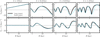 |
Fig. 3 1D radial profiles of the velocity perturbations resulting from the large, m = 2 impact simulation shown in Figure 2. These profiles show VR (top row) and ∆Vϕ (bottom row) as a function of radius R, at the same four times (t = 0, 0.4, 0.8, and 1.2 Gyr). The profiles are averaged on small radial bins at fixed azimuth (ϕ = 0°, corresponding to the dashed-dot regions in Figure 2). The solid black lines represent the results from the large impact simulation. The dashed blue lines show the velocity profiles resulting from the dominant Ω − κ/m wave (specifically the Ω − κ/2 wave for m = 2) in a small impact simulation (extracted from the blue curves in Fig. A.1), scaled up for comparison. These black 1D profiles reveal the characteristic triangular wave shape in VR and the sawtooth pattern in ∆Vϕ, which are key signatures of the non-linear velocity structures generated by the large initial perturbation. |
3 Dynamical discovery with SINDy
Here, we describe our application of SINDy to the simulation time-series data. Our aim is to (re-)discover their governing equations.
3.1 SINDy
SINDy (Brunton et al. 2016) is a data-driven method that extracts the governing equations of a dynamical system directly from measured or simulated data. It is based on the idea that even highly non-linear systems can often be described by equations with only a few dominant terms.
For example, a standard linear ODE system is given by
 (7)
(7)
where x(t) is the state vector and Θ is a constant matrix that characterises the system dynamics. In practice, SINDy extends this framework to non-linear systems by constructing a library x(t) of non-linear candidate functions (e.g. polynomials, trigonometric functions, etc.) and then uses sparse regression to identify the key terms that govern the behaviour. This approach yields a parsimonious model that preserves the physical interpretability of the system. Importantly, the output of SINDy is limited to identifying the best fit among terms provided in its library.
While originally designed for ODEs (ẋ = ƒ(x)), the core sparse regression idea extends to PDEs ut = N(u, ux, uxx,…) by utilising spatial-temporal data (Rudy et al. 2017; Schaeffer 2017). The process involves numerically computing the time derivative (ut) and relevant spatial derivatives (e.g. ux, uxx) from the measured field u(x, t) across all sampled locations and times. These computed derivatives, along with the non-linear combinations of the variables in u, form the library of candidate terms for the right-hand side of the PDE. A summary and example of the methodology is shown in the diagram of Fig. 4, applied to the Navier-Stokes PDE.
3.2 Equations for the small impact evolution
We went on to apply SINDy to the small impact simulations (Sects. 2.1, 2.2). The results of this section are independent of the shape of the initial kick, as long as it is small.
We treated the velocity perturbations, ∆VR and ∆Vϕ, as spatial and time dependent fields, u(R, ϕ, t) = (∆VR, ∆Vϕ). To apply the SINDy PDE approach, we computed the spatial derivatives (∂u/∂R, ∂u/∂ϕ) numerically from the simulation data2. Our library is composed of polynomial combinations, up to second order, of the state variables and their spatial derivatives, expressed as
 (8)
(8)
resulting in a library x(t) of 36 terms. SINDy is then used to identify the sparse combination of candidate terms that best approximates the measured time derivatives across the entire dataset. Since the underlying gravitational potential is axisym-metric, we expect the coefficients of the governing equations to be independent of ϕ, and depend only on R. To capture this, we ran SINDy separately at each radial bin (R). For each radial bin, we combined the data from all ϕ locations within that bin (across all times) to build the SINDy regression problem, allowing us to determine coefficients specific to that radius.
SINDy consistently identified the fact that the dynamics are best described by a linear coupling between the velocity components and their ϕ-derivatives. Specifically, the approach yielded the following equations:
 (9)
(9)
where A(R), B(R), and C(R) are numerical coefficient curves extracted by SINDy at each radial bin. Fig. 5 shows the numerical profiles of these curves (along with a spoiler of the theoretical values we find in Sect. 4). We tested the approach with a variety of potentials and ICs, and observed that the extracted A(R), B(R), and C(R) curves are robust against the different m modes, but do depend on the underlying potential shape. The match between the left side (temporal derivatives) and right side (SINDy library) of both expressions in Eq. (9) is excellent (r2 ~ 1), where the squared correlation coefficient r2 measures the linear correlation between the numerical temporal derivatives and the prediction obtained using the SINDy coefficients, thus showing that SINDy perfectly recovers the governing equations of this system, which motivates our analytical interpretation in Sect. 4.
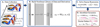 |
Fig. 4 Schematic example of the usage of SINDy to infer the Navier-Stokes equation in a simulation. (A) Collect snapshots representing the solution of the PDE. (B) Compute numerical derivatives and organise the data into a comprehensive matrix Θ that includes the candidate terms for the PDE. (C) Employ sparse regression techniques to isolate the active terms in the PDE. (D) Active terms in the library (x(t), in the text) are informative of the underlying PDE. Reproduced from Brunton & Kutz (2023), who adapted it from Rudy et al. (2017). |
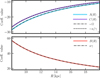 |
Fig. 5 Radial profiles of the coefficients A (blue), B (coral), and C (purple) from the linear PDE system (Eq. (9)) found by SINDy, governing the evolution of velocity perturbations in small impact simulations (Eq. (3)). The black lines show the corresponding analytical values derived in Sect. 4 (Eq. (11)). The excellent agreement between the SINDy-discovered coefficients and the analytical predictions demonstrates the success in recovering the underlying linear dynamics. |
3.3 Equations for the large impact
We went on to perform the SINDy analysis for the large impact simulations (Sect. 2.3, Fig. 2). In this case, where small deviations close to equilibrium can no longer be assumed, we apply SINDy directly to the velocity fields, VR and Vϕ. The library x(t) is thus constructed using VR, Vϕ, their spatial derivatives (∂/∂R and ∂/∂ϕ), and all their second-order polynomial combinations, resulting also in 36 terms.
SINDy extracts a system of equations with a different combination of parameters:
 (10)
(10)

where P(R; m, D) and Q(R; m, D) are numerical coefficients, shown in Fig. 6. The excellent fit (r2~1) indicates that the model captures the dynamics of the system. These coefficients depend not only on the radius and potential but also on the characteristics of the initial impact, namely its shape (mode m) and strength (D), as shown in Fig. 6, where m = 1 (blue) coefficients are different than the m = 2 ones (purple). Consequently, the coefficients in Eq. (10) are specific to the dynamics established by the initial impact parameters (m, D). The method thus captures the dynamics of a specific impact, not a universal law. In Sect. 4.2, we exploit the simple quasilinear structure of Eq. (10) to describe it analytically.
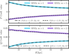 |
Fig. 6 P(R; m, D) and Q(R; m, D) coefficients found by SINDy for the large impact (Eq. (10)) and the corresponding analytical value (Sect. 4.2, Eq. (18)). Since the solution depends on m and D, here we show examples for D = 0.4 and m = 1 (purple) and m = 2 (blue). |
4 Interpreting tidal spirals through the learned equations
In the previous section, we found equations describing the evolution of tidal spirals resulting from small (Eq. (9)) and large impacts (Eq. (10)). SINDy functions provide candidate mechanisms that can then be further analysed and justified through additional experimentation and reasoning. In this way, SINDy serves as a tool to guide us in developing enhanced models and identifying relevant physical mechanisms.
4.1 Small impact equations
For small impacts, the linear PDE system (Eq. (9)) can be derived from linearising the Jeans equations, derivable from the Collisionless Boltzmann Equation (CBE). A complete derivation of this system is given in Appendix B. We reproduce here the resulting linear PDE system for convenience:
 (11)
(11)
These reveal the analytic explanation of the coefficient curves obtained by SINDy in Eq. (9):
 (12)
(12)
In Fig. 5, we show these analytical values on top of the SINDy results.
Equation (11) is equivalent to Eqs. (2b) and (2c) in Lin & Shu (1964) and Eqs. (10) and (11) in Toomre (1964). While similar to these classic equations, our approach differs: they studied self-gravitating propagation from equilibrium ICs, whereas we neglect self-gravity and impose an initial kinematic kick. The analytical solution to this system (see Appendix B.2) is a sum of spiral kinematic waves with frequencies ω = mΩ ± κ:
![Mathematical equation: $\matrix{ {\Delta {V_R}\left( {R,\,\phi ,\,t} \right) = \sum\limits_m {\left[ {{a_m}{e^{i\left( {m\phi - \left( {m\Omega + \kappa } \right)t} \right)}} + {b_m}{e^{i\left( {m\phi - \left( {m\Omega - \kappa } \right)t} \right)}}} \right],} } \hfill \cr {\Delta {V_\phi }\left( {R,\,\phi ,\,t} \right) = \sum\limits_m {\left[ {{c_m}{e^{i\left( {m\phi - \left( {m\Omega + \kappa } \right)t} \right)}} + {d_m}{e^{i\left( {m\phi - \left( {m\Omega - \kappa } \right)t} \right)}}} \right],} } \hfill \cr } $](/articles/aa/full_html/2025/10/aa56039-25/aa56039-25-eq15.png) (13)
(13)
where am, bm, cm, dm are amplitudes determined by the initial conditions, and  . These waves wrap at pattern speeds of
 (14)
(14)
demonstrating the relation (Eq. (4)) that we discussed in Section 2.2. This solution provides an explicit, closed-form description of the temporal evolution of the residual velocities, setting the stage for interpreting the underlying dynamics.
For the weak, impulsive m = 2 case (Struck et al. 2011) discussed in Sect. 2.1, applying the ICs (Eq. (2)) to this framework (see Appendix B.3) shows that the kick decomposes into two waves wrapping at Ω ± κ/2. Their relative amplitude is determined by the potential:
 (15)
(15)
For our fiducial potential, with a γ ≈ 1.46 across the disc, we obtain a ratio of ~5.34, which matches our empirical measurement in Sect. 2.2. Fig. A.1 shows the 1D velocity profiles, illustrating the dominance of the Ω − κ/2 mode.
4.2 Large impact equations
Here, we analyse the non-linear PDE (Eq. (10)) discovered by SINDy in the large impact simulation. Unlike in the small impact case where the SINDy-discovered linear system (Eq. (9)) directly corresponds to the linearised Jeans equations, the non-linear PDE (Eq. (10)) found for the large impact is, as discussed in Sect. 3.3, specific to the ICs and not a general law. Thus, we do not expect a straightforward derivation from first principles. Here we focus on interpreting the dynamics directly through the structure of the PDE identified by SINDy for this particular type of strong perturbation.
We focus our analytical analysis on the azimuthal equation because its structure is ‘self-contained’, meaning that its form depends only on Vϕ and its spatial derivatives, allowing us to determine the evolution of Vϕ independently of VR. SINDy found that both equations in the system (Eq. (10)) share the same coefficients, P and Q. This means that we can derive these key coefficients, applicable to both velocity components, by analysing only one of the equations.
The azimuthal part of Eq. (10) is a first-order quasilinear PDE solvedby the methodofcharacteristics. This means that the quantity Vϕ remains constant along characteristic curves defined by
 (16)
(16)
In Sect. 2.3, we explained that, at each R, the minimum Vϕ corresponds to the apocentre of an inner orbit with guiding radius Rg,in, and moves at a constant pattern speed Ω(Rg,in) – κ(Rg,in)/m. Similarly, the points where Vϕ = Vc move at a constant pattern speed Ω(R) − κ(R)/m. These associations provide two constraints on the coefficients P and Q. By equating the instantaneous pattern speed from the characteristic curve (Eq. (16)) to the expected pattern speed for two specific constant Vϕ values, we arrive at the following system of equations:
 (17)
(17)
where the first equation corresponds to the apocentres (Vϕ= Vc − DR/γ, minimums in Eq. (6)), that evolve with pattern speed Ω(Rg,in) − κ(Rg,in)/m and the second equation corresponds to points where Vϕ = Vc, with pattern speed Ω(R) − κ(R)/m.
Solving this system yields a closed form for the PDE coefficients
 (18)
(18)
where we defined ∆Ω ≡ Ω(Rg,in) − Ω(R) and ∆κ ≡ κ(Rg,in) − κ(R). In Fig. 6, we show that these curves match perfectly with the coefficients extracted by SINDy, providing strong validation for both the SINDy discovery and our analytical interpretation.
Crossing time. The characteristic curves of the system reveal an important dynamical aspect: their eventual crossing. In the astrophysical context, this corresponds to the appearance of overlapping kinematic populations in the same spatial volume, which challenges the definition of a unique “mean velocity” and, ultimately, the assumptions in the Jeans equations.
From Zachmanoglou & Thoe (1986), we can extract, for a PDE with the shape of Eq. (10), an overlap or crossing time of
 (19)
(19)
meaning that the earliest crossing originates at the point ϕc where the derivative of the initial condition Vϕ,0 (Eq. (6)) is the most negative. This gives us a closed expression for the crossing time:
 (20)
(20)
Even in simulations where the Sgr impact on the velocities at the Solar neighbourhood is on the larger side of the spectrum (∆VR, ∆Vϕ~25 km s−1), this would translate to D ~ 2. In our framework, this yields tcross ≳ 1.5 Gyr, comfortably exceeding the estimate of the last Sgr passage (≲1 Gyr). Indeed, Hunt et al. (2024) showed that, for a kick compatible with a Sgr passage, the wraps of the radial phase spiral appear at least after ~1 Gyr. Thus, in the context of a Sgr passage, we do not expect a crossing of the perturbed populations.
5 Applying SINDy to more realistic simulations
We went on to test our method on a more realistic N-body simulation of a Sgr-like impact and a test-particle rerun (TPR) of the same simulation (Asano et al. 2025, and in prep.), initialised with particles from the same snapshot but evolved in a fixed axisymmetric potential. Running SINDy on these models allows us to test the method in more complex 3D setups with velocity dispersion and self-gravity. Details of these simulations can be found in Appendix D.
Figure 7 shows the velocity maps for the N-body (first and third columns) and TPR (second and fourth columns) models over a ~250 Myr period after the first Sgr pericentre. A bar dominates the inner disc (R < 7 kpc), so we focus on the outer region (R > 7 kpc). In this outer region, we see similar patterns to those discussed in Sect. 2.3 with our idealised test particle models with large impact. We observe a winding spiral with pattern speed Ω − κ/m, which we measured using Fourier decomposition. This spiral pattern also displays characteristic non-linear features: regions with negative VR (blue) tend to concentrate, and the Vϕ profile develops sharp edges. These realistic simulations, however, also reveal additional substructure (e.g. thin arches, bifurcations) that differs from the simplified idealised models. Finally, we observe subtle differences between these two models in Fig. 7, primarily a larger amplitude of the kinematic waves in the N-body simulation at t = 1.15 Gyr. This difference could be related to the self-gravity of the spiral arms and/or the extra acceleration of the perturber after the pericentre, which are not included in the TPR model.
5.1 SINDy results
We then applied the large-impact SINDy analysis (Sect. 3.3) to the TPR and N-body models. In both models, from a library of 36 terms, SINDy successfully recovered the exact same structural form of the non-linear PDE (Eq. (10)). This striking consistency demonstrates the robustness of the method.
In Fig. 8 we show the P (first row), and Q (second row) coefficients obtained by SINDy in the TPR (blue) and N-body models (purple), as well as the analytical prediction (Eq. (10)). The left (right) column shows the coefficients obtained when fitting the radial (azimuthal) part of the non-linear PDE (Eq. (10)). Although the coefficient P should be identical in the radial and azimuthal equations (same for Q), SINDy fits them independently, allowing for different results. The bottom row of Fig. 8 shows the r2 value. This value indicates how good the SINDy model fits the data at each radius. In both cases, the fit is sub-optimal (r2 < 0.7). This points to missing terms in our library.
For the TPR model (blue lines in Fig. 8), the recovered coefficients match the expected ones (dashed-dot lines, Eq. (18)) fairly good, with the exception of some coherent oscillations in R. For the N-body simulation (purple lines in Fig. 8), the recovered coefficients are similar to the ones recovered from the TP rerun in the radial equation, but differ significantly in the azimuthal direction. We discuss the possible causes of this deviation in the following section.
5.2 Limitations of the method
The suboptimal r2 fitting of the coefficients recovered by SINDy in the realistic models (bottom row in Fig. 8) reveals significant limitations in our approach. Compared to the idealised setup (Sect. 2.3), the realistic models introduce complexities such as vertical motion, velocity dispersion, different (more complex) initial conditions (e.g. Semczuk et al. 2025), and self-gravity. These factors are potentially responsible for the reduced goodness-of-fit.
Vertical motion. Our analysis (Sect. 3.3) uses a 2D model. However, the disc in the TPR and N-body models is 3D. We tested the impact of the vertical motion by applying SINDy to a subsample of particles with small |Z| and |VZ| from the TPR model. The recovered coefficients were nearly identical to those from the full sample. This suggests that, in this specific simulation and time frame, the vertical motion is likely not the primary cause for the suboptimal fit of the equations.
Velocity dispersion. In A22, we studied test particle simulations with a significant velocity dispersion, and showed that the pattern speed of the spiral arms and the evolution of the system is very similar to our idealised models. However, velocity dispersion fundamentally alters the dynamics by introducing pressure-like terms into the Jeans equations. This physical effect, which is absent in our cold-disc model, would require expanding the SINDy library to include terms related to the velocity dispersion tensor. The complexity is further compounded by the fact that real Galactic discs are composed of multiple stellar populations, each with its own characteristic velocity dispersion. Therefore, these factors likely contribute to the residual error and the suboptimal r2 values observed in Fig. 8.
ICs. The ICs in the realistic simulations are taken at t = 0.9 Gyr, reflecting the full dynamical history (tidal impact, bar, previous spiral arms, etc.). This differs from the idealised analytic kick assumed for the theoretical coefficients (Eq. (6)) that determines the values of the Pm,D and Qm,D coefficients. Consequently, the recovered coefficients in Fig. 8 are not expected to perfectly match the analytical predictions across all radii.
Self-gravity. The main discrepancy between the coefficients extracted from the TPR and N-body models is observed in the azimuthal equation (right column in Fig. 8). We hypothesise that this discrepancy is driven by the self-gravity of the spiral arms. For loosely wound spirals, as in the temporal range we consider (Fig. 7), the self-gravity acceleration is more dominant in the azimuthal direction than in the radial direction (Lin & Shu 1964). It is also important to notice that the radius where the difference between the TPR and N-body coefficients is larger, R = 10 kpc, corresponds to the Outer Lindblad Resonance radius of the bar. While this alignment may be coincidental, it raises the possibility that the bar is contributing to the discrepancy between the SINDy results and theoretical predictions.
Missing terms in the library. The consistently low r2 values in Fig. 8 (bottom row) are the strongest indication that the equation discovered by SINDy (Eq. (10)) is missing important physics, such as velocity dispersion and self-gravity. While it is difficult to determine the precise contribution of each, these terms are necessary components of the full Jeans equations that govern disc dynamics, and capturing a more complete dynamical description in the future will require expanding the SINDy library to include them.
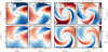 |
Fig. 7 Kinematic maps comparing the evolution of velocity fields in the N-body (first and third columns) and TPR models (second and fourth columns). The panels show snapshots of the radial velocity VR (top row) and the azimuthal velocity perturbation ∆Vϕ (bottom row) in the X–Y plane at two different times. The dashed circle denotes the inner region (R < 7 kpc) that was excluded from the analysis. Observe the winding of the spiral patterns over time and the overall similarity between the N-body and TPR models, with subtle differences, particularly in the amplitude of the kinematic waves. |
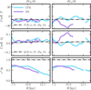 |
Fig. 8 Results from applying SINDy to the TPR (blue lines) and N-body (purple lines) models. The top row shows the SINDy-recovered coefficient P, and the middle row shows coefficient Q, both as a function of R. The bottom row shows the r2 value, indicating the goodness-of-fit for the SINDy model at each radius. The black dash-dotted lines represent the analytical predictions for P and Q (Eq. (18)). The coefficients P and Q obtained by fitting the radial derivative (∂VR/∂t) and the azimuthal derivative (∂Vϕ/∂t) are shown in the left and right columns, respectively. Voids in the curves correspond to radii where SINDy failed to find a solution. |
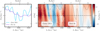 |
Fig. 9 Best fit of an impulsive m = 2 perturbation to the Gaia DR3 Lz − ϕ − 〈VR〉 map. Left panel: 〈VR〉 as a function of Lz for Gaia DR3 data (blue) and the best fit model (purple), at ϕ = 0° (dot-dashed line in the other panels). Middle panel: The Lz − ϕ map of 〈VR〉 for Gaia DR3 data. Right panel: Lz − ϕ map of 〈VR〉 for the best fit model. The dashed curve indicates the 〈VR〉 = 0 km s−1 curve of the data. |
6 The Gaia Lz −〈VR〉 wave
Friske & Schönrich (2019) showed a clear wave in the Lz − VR projection of the Gaia data (studied also in A22, Cao et al. 2024). They found a short and a long wavelength pattern with similar amplitudes (𝒜1 = 7.0 km s−1 and 𝒜2 = 8.0 km s−1), and differing wavelengths (λ1 ~ 285 kpc km s−1 and λ2 ~ 1350 kpc km s−1). The presence of these two waves, combined with the two wave pattern (Ω ± κ/2) observed in Sect. 2 from a single impact, raises a clear question: could we explain the full LZ−〈VR〉 wave with a simple impulsive impact like that of a single Sgr passage?
To investigate this, we start by examining the LZ−〈VR〉 wave in Gaia DR3 data3 (blue curve in the left panel of Fig. 9). We also plot the mean radial velocity 〈VR〉 in the Lz − ϕ plane (central panel in Fig. 9, also shown in Chiba et al. 2021, A22). We observe patterns consistent with previous findings, showing diagonal features in the Lz − ϕ plane, potentially indicative of spiral structure. We test the simplest scenario that could produce these signatures: a single distant impulsive Sgr passage (Eq. (2)). Using the analytical solution for an m = 2 impulsive kick (derived in Appendix B.3), we constructed VR = ƒ(LZ, ϕ; t, ϵ, ϕ0, VR,0) to fit the 〈VR〉 of the observations. This model is a specific case of Eq. (13) where the amplitudes of the two m = 2 waves depend only on the impact strength ϵ (Eq. (B.16)). Here, t is the time since the impact, ϵ is the impact strength, ϕ0 is the initial angle of the perturber, and VR,0 is a constant offset in VR (equivalent to the t parameter in Eq. (2) in Friske & Schönrich 2019). The fit is done by minimising the squared difference between the model and data4.
The right panel of Fig. 9 shows the best-fit model map in the LZ − ϕ plane, and the purple curve in the left panel shows the corresponding Lz−〈VR〉 profile at ϕ = 0°, compared to the Gaia data (blue curve). The best values we found for the model parameters are:

The values obtained are quite reasonable. For instance, the fitted time t is roughly consistent with estimates for the time of impact derived from fitting the vertical phase spiral (Antoja et al. 2018; Frankel et al. 2023; Antoja et al. 2023; Darragh-Ford et al. 2023). The initial angle ϕ0 is not well constraint by the fit. For the impact parameter ϵ, which can be approximated by  (Sect. 2.1), we see that, using the values for the last pericentre from Vasiliev et al. (2021), rp ~ 24.3 kpc and υp ~ 281 km s−1, our fitted value implies a Sgr mass estimate of Mp ~ 1.17 × 10¹⁰ M⊙, which is one order of magnitude larger than the total mass estimated at the last pericentre (Vasiliev et al. 2021). The need for a higher mass of Sgr to reproduce the observables has already been pointed out in other studies (e.g. Binney & Schönrich 2018; Laporte et al. 2019). However, these mass estimates remain inconclusive due to the unconstrained mass loss history of Sgr.
More importantly, this model (and, thus, the obtained parameters) comes with several limitations. The impulsive kick model predicts a large amplitude difference between the two waves (~5.34, Eq. (15)), while in the Gaia data, these amplitudes are much more similar (~1.14). This means that the model cannot reproduce the observed balance between the two wave components. This is seen in the difference between the ‘short’ waves in the left panel of Fig. 9. Another limitation is the use of the linear model instead of the non-linear equations. However, for the time and amplitude range of the fitting, we only expect small second-order corrections to the shape of the wave (see central panels of Fig. 3), and thus this would not be a significant issue. Finally, the limitations discussed in Sect. 5.2 also apply here; thus, accounting for the velocity dispersion or self-gravity effects could influence the fitting results.
In addition, our model is only considering a single, impulsive passage, but could be extended or combined with complementary dynamical processes. These could include the effect of multiple Sgr passages, each one generating one of the observed waves, as we explored in A22: closer non-impulsive perturbations; the combined influence of the Galactic bar and stellar spiral arms (e.g. Hunt et al. 2019; Khalil et al. 2025); or the cumulative effect of other past or present perturbers. Despite all the listed limitations, both the obtained fitting and parameters are promising results, pointing to a potential diagnostic of the Sgr passage using planar motions. We aim to explore this model in detail in future work.
7 Discussion
7.1 Potential of the method
Applying data-driven discovery tools like SINDy to simulations offers significant potential, serving as an empirical guide or providing simplified descriptions in complex regimes. In the case of the small-impact simulations, SINDy identified the linear PDE system. This system is known to describe the evolution of perturbations in a collisionless disk (e.g. Toomre 1964; Lin & Shu 1964). The significance here is not the novelty of the equation itself, but the ability of the method to extract this fundamental structure directly from the simulated phase-space data. This success served as a validation of the SINDy approach for this type of problem and provided the empirical foundation that guided our analytical derivation (Sect. 4), enabling us to obtain explicit, closed-form solutions describing the phase-space distribution at all times (Eq. (13)). The performance of SINDy depends critically on the temporal resolution of the data. While, obviously, the sampling must resolve the characteristic timescales of the system for SINDy to reproduce them, usually the challenge is ensuring the numerical stability of the time derivatives. In our analysis, we carefully checked that the fine time steps used were sufficient to obtain smooth and stable derivatives for both VR and Vϕ. In general, however, each application of the method will have its own requirements that need to be assessed.
For the specific large-impact scenario, SINDy discovered a non-linear PDE system (Eq. (10)) governing the kinematic perturbations. To our knowledge, this particular form has not been explicitly discussed previously in the context of galactic dynamics. Although this equation is specific to the used ICs and not a general law like the Jeans equations, its surprising simplicity – notably the absence of explicit radial derivatives and a single non-linear term – contrasts with the complexity of the full Jeans equations required to model this regime. This simpler structure directly facilitated the theoretical analysis of features like the characteristic curves and the derivation of the crossing time (Eq. (20)). Applying SINDy to realistic simulations (Sect. 5) recovered the same PDE structure, demonstrating the method robustness to velocity dispersion, 3D motion, and complex histories. The discrepancies in the recovered coefficients (Fig. 8) are a valuable outcome, pointing to missing physics (like self-gravity, as discussed in Sect. 7.2) and guiding the systematic improvement of our models.
The governing PDEs we have identified also open up a route for efficient forward modelling. Instead of running full particle simulations or numerically solving PDEs directly, one can transform the PDEs into systems of coupled ODEs by expanding the dynamical fields in a basis of functions. This approach, characteristic of spectral methods, allows for faster evolution of the system in coefficient space, and is closely related to the latest developments in galactic dynamics (Rozier et al. 2019; Petersen et al. 2024). We demonstrate this technique for the linear PDE system and show its effectiveness in Appendix C. While more complex for the non-linear case, solving the resulting ODE system still offers significant computational advantages over traditional methods.
7.2 Adding self-gravity to the mix
Our current simplified PDE (Eq. (10)) does not explicitly include terms representing the self-gravitational forces or the potential response of the live halo (Bernet et al. 2025). This introduced discrepancies when applying SINDy to more realistic simulations (Sect. 5, Fig. 8). The data-driven discovery framework, however, offers clear paths to address these limitations. One approach is to explicitly calculate the gravitational acceleration due to the evolving self-consistent density structure of the spiral arms (and potentially other components such as the live halo or external perturber). These calculated accelerations could then be included as additional terms in the SINDy library, treating the self-gravity as an external force acting on the system.
Another clear path to extend the SINDy library is to include terms related to the density field itself. The method could potentially uncover a different, more comprehensive set of PDEs. We hypothesise that SINDy might identify a PDE structure that intrinsically accounts for the self-gravitational forces, potentially finding a more effective or simplified representation than the full, complex Jeans equations required for the coupled density-velocity system. Beyond self-gravity, these data-driven techniques could also prove powerful for uncovering tractable, scenario-specific models of complex effects such as dynamical friction–especially difficult to solve analytically—just as SINDy identified a relatively simple non-linear PDE (Eq. (10)) for the large-impact case. In addition, SINDy is closely related to other data-driven dynamical analysis methods, such as Dynamic Mode Decomposition (DMD, Schmid 2010, see Brunton et al. 2016). DMD identifies dominant system modes and has been applied to simulations of vertical phase spirals (Darling & Widrow 2019). In a similar direction, our methodology could be extended to model the full 3D response of the disc. Running the methodology in a similar setup, with a vertical (instead or in addition to the planar) perturbation, we could study the phase-mixing of bending waves, and their coupling with the planar dynamics, complementing, for example, the approaches of Chequers et al. (2018); Bland-Hawthorn & Tepper-García (2021); Asano et al. (2025).
7.3 Application to observational data
In Section 6, we applied our analytical model for an impulsive kinematic kick (derived from the linear PDE, Eq. (13)) to fit the observed LZ−〈VR〉 wave in Gaia data. Fig. 9 shows that this simple model can reproduce the overall structure and winding pattern of the observed wave reasonably well, providing specific parameters for the Sgr passage time and strength, although several key limitations are mentioned. The idea of analysing kinematic wave structures, such as the Lz − VR wave, can be generalised to model similar phenomena in external galaxies. The increasingly precise kinematic maps, obtained through integral field spectroscopy (e.g. Erroz-Ferrer et al. 2015; Cappellari 2016; den Brok et al. 2020), and even using Gaia data in the LMC (Jiménez-Arranz et al. 2023, 2024, 2025), provide rich datasets of kinematic information. These datasets contain several examples of tidal features and kinematic waves, but cleanly distinguishing tidally induced spirals from those generated by other mechanisms (e.g. bars or internal instabilities) remains a key open question.
The morphology of spiral arms is known to be linked to the properties of the host galaxy, exemplified by the correlation between pitch angle and galactic shear rate (Γ) in the context of transient, corotating spiral arms (e.g. Lin & Shu 1964; Seigar et al. 2005; Grand et al. 2013). The dynamics of the tidally-induced arms in our model are naturally consistent with this observational trend. The connection is direct: the pattern speeds we study, Ωp = Ω ± κ/m, are a function of shear via the relation κ2 ∝ Ω2(2 − Γ). Consequently, a higher shear rate leads to more rapid differential winding and intrinsically tighter arms5. However, since the pitch angle in our model also depends on the time elapsed since the impact, we expect these arms to populate the relation with a significant scatter, corresponding to their evolutionary stage.
This evolutionary sequence implies a wide range of pitch angles, starting open and becoming progressively tighter. However, because the initial perturbation is purely kinematic, a density contrast only builds as the arms wrap, setting a practical maximum boundary on their observable pitch angle in density tracers. Conversely, the finite lifetime of the arm sets a minimum boundary. In our idealised model, this lifetime is marked by the kinematic winding into an unresolvable pattern or, for large impacts, by the non-linear crossing time (tcross, Eq. (20)). In more realistic setups, this would be further accelerated by the velocity dispersion. Together, these effects define an observable window of pitch angles, though estimating its boundaries is complex, as it depends on the kick strength, host galaxy properties, and observational resolution. It is plausible that the observed spiral arm population is a mix of types, with the observed correlation possibly dominated by more isolated galaxies. This opens a powerful diagnostic avenue: using the morphology of tidal arms to independently constrain the gravitational potential of a galaxy and its interaction history.
8 Summary and conclusions
The spiral structure and overall dynamics of the MW remain a major area of research, with recent observations highlighting that the MW disc is not in a steady state but is actively perturbed, likely by the passage of the Sgr dwarf galaxy. In this work, we explored the dynamics of tidally induced spiral arms applying SINDy, a data-driven technique that identifies the governing differential equations of a dynamical system directly from simulation data. Our main findings are summarised below:
A single m-fold impulsive velocity kick with small amplitude triggers the formation of two m-armed spiral waves, wrapping at pattern speeds of Ω ± κ/m. The amplitudes of these waves depend on the shape of the initial kick and the potential, and can be analytically described (Sect. 4);
Applying SINDy to simulations of small impacts, we successfully recovered the linear PDE (Eq. (9)) governing the evolution of the system, validating the capability of the method;
Guided by the SINDy discovery, we analytically re-derived the linear PDE system from first principles using the CBE. This derivation recovers equations equivalent to classical descriptions (Toomre 1964; Lin & Shu 1964) and provides a closed-form solution (Eq. (13)) of the temporal evolution of the VR and Vϕ maps;
We defined a family of simplified larger impacts (Eq. (6)) resulting in m-armed spiral patterns. For these cases, SINDy discovered a simple, previously unknown non-linear PDE system (Eq. (10)), which describes the evolution of the system, demonstrating its potential to uncover simplified governing equations in complex regimes;
The coefficients of the non-linear PDE (Eq. (10)) are specific to the initial impact characteristics (mode m, strength D), highlighting that this equation describes the dynamics for a particular type of perturbation, not a universal law. However, its simple mathematical structure enables the interpretation of its characteristic kinematic features;
The analysis of the non-linear PDE (Eq. (10)) provides a framework for interpreting the characteristic kinematic patterns observed in simulations (e.g. triangular VR and saw-tooth Vϕ profiles in Fig. 3), which resemble features in MW phase space (e.g. the R − Vϕ ridges and Lz − VR wave). Our interpretation of this PDE through characteristic curves reveals that these patterns arise from differential wrapping;
Applying our data-driven framework to more realistic simulations (an N-body simulation and its test-particle rerun), we successfully recovered the same non-linear PDE structure (Eq. (10)) found in idealised simulations, demonstrating the potential of this method in more complex setups;
The coefficients recovered from the realistic simulations showed discrepancies compared to idealised cases (Fig. 8), which we attribute primarily to physical effects that are not explicitly included in our simplified PDE, such as self-gravity;
We applied the closed-form solution (Eq. (13)), assuming a simple impulsive kick, to fit the Gaia LZ−〈VR〉 wave (Sect. 6). We obtained reasonable visual fit and parameters for a Sgr passage, including a passage time of ~ 0.42 Gyr and an inferred perturber mass ~1.17 × 10¹⁰ M⊙. However, our model shows a significant discrepancy in the amplitude ratio between the two main observed components. This mismatch suggests that the simple assumption of a single impulsive kick is an incomplete description of the LZ−〈VR〉 wave. The discrepancy could arise from the limitations of this simplified model of the Sgr encounter, or it may indicate a more complex physical origin for the waves, such as multiple passages or the influence of other galactic components, such as the bar.
The evolution of the field of galactic dynamics, increasingly data-driven, demands new methods for studying the fundamental principles governing non-equilibrium dynamics. Our approach offers a new path to explore theoretical dynamics often intractable otherwise. It complements other novel data-driven techniques in the field, such as Orbital Torus Imaging (OTI, Price-Whelan et al. 2021, 2025; Horta et al. 2024; Oeur et al. 2025) for constraining the gravitational potential, basis function expansions (Johnson et al. 2023; Arora et al. 2024, 2025) for efficient dynamical field evolution, and neural network-based potential recovery from kinematics (Green et al. 2023; Kalda et al. 2024; Zucker et al. 2025). These frameworks link empirical data to predictive analytical models, offering a direct path for exploring theoretical dynamics and dissecting complex galactic structure and evolution, including challenging phenomena such as self-gravity and dynamical friction.
Acknowledgements
We thank the anonymous referee for their constructive report. We thank Kathryn V. Johnston, Chris Hamilton, Kiyan Tavangar, the EXP collaboration, especially the Bars & Spirals working group, and the Gaia UB team for the valuable discussions that contributed to this paper. We acknowledge the grants PID2021-125451NA-I00 and CNS2022-135232 funded by MICIU/AEI/10.13039/501100011033 and by “ERDF A way of making Europe”, by the “European Union” and by the “European Union Next Generation EU/PRTR”, and the Institute of Cosmos Sciences University of Barcelona (ICCUB, Unidad de Excelencia ’María de Maeztu’) through grant CEX2019-000918-M. MB acknowledges funding from the University of Barcelona’s official doctoral program for the development of a R+D+i project under the PREDOCS-UB grant. T.A. acknowledges the grant RYC2018-025968-I funded by MCIN/AEI/10.13039/501100011033 and by “ESF Investing in your future”. This research in part used computational resources of Pegasus provided by Multidisciplinary Cooperative Research Program in Center for Computational Sciences, University of Tsukuba.
Appendix A Radial profiles of the small impact
This appendix presents supplementary details and visualisations of the velocity structure resulting from the small, distant m = 2 kinematic kick simulation discussed in Section 2.1. Fig. A.1 shows the 1D radial profiles of the velocity perturbations ∆VR (top row) and ∆Vϕ (bottom row) as a function of radius R, specifically along the line ϕ = 0°, at five different times (t = 0, 0.1, 0.2, 0.3, 0.4 Gyr). Each panel breaks down the total velocity perturbation (black line) into the contributions from the two fundamental wave modes excited by the m = 2 kick: the Ω − κ/2 mode (blue line) and the Ω + κ/2 mode (purple line). These profiles visually demonstrate how the initial kick at t = 0 Gyr is composed of these two modes and how the spatial structure evolves over time. Notably, the Ω − κ/2 mode contributes significantly to the overall perturbation pattern, while the Ω + κ/2 mode is typically seen as smaller-scale radial variations superimposed on the dominant mode.
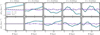 |
Fig. A.1 Radial profiles of velocity perturbations ∆VR (top row) and ∆Vϕ (bottom row) for the small, distant, m = 2 kinematic kick simulation (Sect. 2.1), as a function of R, at four different times, at ϕ = 0°. In each panel, the blue line represents the contribution from the Ω − κ/2 wave, the purple line represents the Ω + κ/2 wave, and the black line is the sum of these two modes, which corresponds to the total velocity perturbation at that radius. The initial kick (t = 0 Gyr) decomposes into the two modes. As time evolves, the Ω − κ/2 mode remains dominant and shapes the overall perturbation pattern, while the Ω + κ/2 mode appears as smaller-scale radial oscillations on top of it. |
Appendix B Analytical derivations
B.1 Derivation of the linear equations
We start by considering the Collisionless Boltzmann Equation in 2D Cylindrical Coordinates, for an axisymmetric potential without self-gravity:
 (B.1)
(B.1)
Taking moments by multiplying by υR and υϕ and integrating over the velocities yields the Jeans Equation for the mean velocities VR and Vϕ. We assume there is no velocity dispersion, so all stress-tensor terms drop out, matching the zero-dispersion setup of our simulations (Sect. 2). This yields:
 (B.2)
(B.2)
We linearise the equation by assuming a small perturbation about the equilibrium of the form Vϕ = Vc(R) + ∆Vϕ, VR = ∆VR:
 (B.3)
(B.3)
where  . Assuming
  and
and  , we can rewrite the linearised equations to obtain the following system of equations:
 (B.4)
(B.4)
In the following section, we derive the analytical solution of the linear PDE recovered here (Eq. B.4).
B.2 Solution of the linear equations
For a fixed radius R, where Ω(R), κ(R), and γ(R) are constants, the linearised system (Eq. B.4) becomes a pair of linear PDEs with constant coefficients. Exponential functions like ei(mϕ−ωt) are eigenfunctions of linear differential operators, simplifying the PDEs to algebraic equations. Therefore, we can assume solutions of the form
 (B.5)
(B.5)
where m is the azimuthal mode and ω is their frequency. Substituting these solutions in the linearised system and operating it, we obtain
 (B.6)
(B.6)
whose solution leads to the relation
 (B.7)
(B.7)
which tell us which eigenfunctions “survive”, i.e. which waves develop after the initial perturbation. The pattern speed of these waves (Ωp ≡ ω/m) is then
 (B.8)
(B.8)
Finally, solving Eq. B.6 also gives the amplitude relation
 (B.9)
(B.9)
where the inverted ∓ sign means that it is the opposite sign as the one obtained for Ω ± κ/m. Therefore, the analytical solution of the system consists of a sum of spiral density waves with frequencies ω = mΩ ± κ:
![Mathematical equation: $\matrix{ {\Delta {V_R}\left( {R,\,\phi ,\,t} \right) = \mathop \sum \limits_m \left[ {{a_m}{e^{i\left( {m\phi - \left( {m\,\Omega + \kappa } \right)t} \right)}} + {b_m}{e^{i\left( {m\phi - \left( {m\,\Omega - \kappa } \right)t} \right)}}} \right],} \hfill \cr {\Delta {V_\phi }\left( {R,\,\phi ,\,t} \right) = \mathop \sum \limits_m \left[ {{c_m}{e^{i\left( {m\phi - \left( {m\,\Omega + \kappa } \right)t} \right)}} + {d_m}{e^{i\left( {m\phi - \left( {m\,\Omega - \kappa } \right)t} \right)}}} \right],} \hfill \cr } $](/articles/aa/full_html/2025/10/aa56039-25/aa56039-25-eq38.png) (B.10)
(B.10)
where am, bm, cm, dm are amplitudes determined by the initial conditions, and  .
.
B.3 Small m = 2 impact
The initial velocity kick by the perturber from Equation 2 with a simple m = 2 mode with small amplitude can be written in compact, complex notation, as the real parts of
 (B.11)
For an m = 2 mode, using the general solution (Eq. B.10) obtained in the previous section, we write
 (B.12)
At t = 0, the solution must match the initial conditions, that is:
 (B.13)
 (B.14)
where we used the eigenmode relation  . This immediately gives
 (B.15)
Solving these two simple equations for a2 and b2, we obtain the amplitude of the surviving modes
 (B.16)
Substituting these amplitudes, along with the corresponding  and
and  , back into the general solution form (Eq. B.12) shows the time evolution of the perturbation:
 (B.17)
These expressions clearly show that the initial impulsive condition at t = 0 has decomposed into a superposition of two distinct waves, with amplitudes a2 and b2. Thus, the relative amplitude of these waves is directly determined by
 (B.18)
where we used that γ > 1 to remove the absolute values.
Appendix C Basis Function evolution
The linear PDE system (Eq. B.4) obtained in Sect. 4 (Appendix B.1) governs the evolution of the small impact system. We can solve this PDE system efficiently by expressing the velocity perturbations in terms of coefficients from a basis function expansion. Using this method, the linear PDE system is transformed into a system of coupled ODEs for the time-dependent coefficients, allowing us to evolve the system “only” in the coefficient space.
We expand the perturbations ∆VR(R, ϕ) and ∆Vϕ(R, ϕ) in an orthonormal basis function. For the angular direction, we use the full complex Fourier basis, while in the radial direction we adopt a general orthonormal basis {Gn(r)} defined on the interval Rmin ≤ r ≤ Rmax. That is, we write
 (C.1)
(C.1)
where the angular and radial basis functions are given by
 (C.2)
(C.2)
and the radial basis functions satisfy the orthonormality condition
 (C.3)
(C.3)
Assuming that the quantities ∆VR, ∆Vϕ evolve in time according to Eq. B.4, we substitute them by our basis functions equations (Eq. C.1). Below we show an example of how we proceed with the  term. Since it is a linear system, the calculation is equivalent for all the other terms of the system.
After inserting the basis expansion, the  term takes the form
 (C.4)
(C.4)
where we have used that  . To isolate the evolution of a particular coefficient αm,n(t), we project this expression onto the basis by multiplying it by
  and integrating over the entire domain
![Mathematical equation: $\int_0^{2\pi } {d\phi \,\,\int {r\,dr\,u_m^*\left( \phi \right)\,{G_n}\left( r \right)\left[ {\sum\limits_{m',n'} {{\alpha _{m',n'}}\left( t \right)\,{u_{m'}}\left( \phi \right)\,\Omega \left( r \right)\,{G_{n'}}\left( r \right)} } \right].} } $](/articles/aa/full_html/2025/10/aa56039-25/aa56039-25-eq59.png) (C.5)
(C.5)
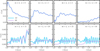 |
Fig. C.1 Temporal series of the basis function coefficients after a small m = 2 impact (Sect. 2). In blue, we show the basis function coefficient at each snapshot of the test particle simulation. In purple, we initialize the coefficients αm,n(t = 0) and βm,n(t = 0) analytically and evolve them using Eq. C.10. |
Due to the orthonormality of the angular basis functions um(ϕ), the expression simplifies to
 (C.6)
(C.6)
where the radial coupling integral is defined by
 (C.7)
(C.7)
One can proceed identically with the rest of the terms in Eq. B.4. Only the terms with ∂/∂ϕ have the i m factor. The derivation for the left part of the system, the temporal derivatives, leads to a coupling integral
 (C.8)
(C.8)
where the identity matrix appears due to the orthonormality of the radial basis.
After the projection of the entire system, the time evolution of the expansion coefficients corresponding to a given angular mode m can be written as a system of coupled ODEs:
 (C.9)
(C.9)
where (κγ)n,n′ and (κ/γ)n,n′ are constructed using an analogue to Eq. C.7. In compact block-matrix notation for each m, this system is expressed as
 (C.10)
and can be solved numerically (e.g. using matrix exponentiation). This conversion of PDEs into ODEs using basis function expansion (BFE) is a core technique in galactic dynamics, often used in spectral methods and the response-matrix framework (e.g. Kalnajs 1971; Rozier et al. 2019, 2022; Petersen et al. 2024). It transforms the differential operators in the PDE into algebraic operations on the time-dependent basis coefficients, allowing for efficient time evolution directly in coefficient space.
In Fig. C.1 we show the evolution of different n coefficients of the orthogonal basis function for the test particle simulation (TP, blue lines). For this run, we used a Legendre polynomial basis in the radial direction. Using the analytical impact formula, we compute the initial αm,n, /βm,n coefficients, and evolve them using Eq. C.10 (BF, purple lines). We observe a great match between both methods in the low order coefficients. In the high order coefficients, we notice that we can go well below the noise threshold, and still capture a significant signal. This demonstrates the accuracy and efficiency of evolving the system in coefficient space for the linear case.
Applying this spectral approach to the SINDy-discovered non-linear PDE for the large-impact scenario (Eq. 10) is more challenging than the linear case because non-linear terms introduce complex couplings between the basis coefficients. However, solving the resulting system of ODEs for the coefficients would still be significantly faster than running full particle simulations or solving the non-linear PDE numerically. This method could be applied to more complex SINDy-discovered PDEs, perhaps including self-gravity terms, offering an efficient way to explore the parameter space of galactic perturbations.
Appendix D Realistic Simulation Details
This appendix provides detailed information about the realistic simulations used in Section 5.
N-body simulation. We use the N-body simulation of a Sgr-like impact, presented in Asano et al. (2025), which is an extension of the original models described in Fujii et al. (2019). In this model, the MW-like host galaxy is constructed with a three-component structure: a DM halo, a classical bulge, and an exponential stellar disc. The DM halo follows an NFW profile (Navarro et al. 1996) with a scale radius of 10 kpc and a mass of Mh = 8.68 × 10¹¹ M⊙. The bulge is modelled with a Hernquist (1990) profile having a scale radius of 0.75 kpc and a mass of 5.42 × 10⁹ M⊙. The stellar disc is characterised by an exponential radial profile with a scale radius of 2.3 kpc, a vertical scale height of 0.2 kpc, and a total mass of 3.61 × 10¹⁰ M⊙. The stellar disc contains 213M particles. The Sgr-like satellite has a DM component that follows an NFW profile with a total mass of 5 × 10¹⁰ M⊙ and a scale radius of 7.5 kpc, while its stellar component is represented by a Hernquist profile with a mass of 1 × 10⁹ M⊙ and a scale radius of 2 kpc.
From this simulation, we select the time range starting 250 Myr after the first pericentre (t = 0.9 Gyr) for our analysis. This period resembles the tidal spiral phase before the appearance of kinematic crossings (Eq. 20) becomes significant.
Test Particle Rerun TPR. Complementing this N-body simulation, Asano et al. (in prep.) have run a suite of test particle reruns of the previous N-body model using Agama. Here we used one of them, which we call TPR, to isolate and test the contribution of self-gravity to the SINDy analysis compared to a frozen potential. In this run, the initial conditions (ICs) of the disc particles are those of the N-body at the first pericentre time (t = 0.9 Gyr). The particles are then evolved in the isolated frozen axisymmetric potential of the MW host galaxy, effectively removing the self-gravity of the disc and halo, as well as the external acceleration from the perturber. The evolution of this simplified model is shown alongside the N-body maps in the second and fourth columns of Fig. 7.
References
- Aguilar, L. A., & White, S. D. M. 1985, ApJ, 295, 374 [NASA ADS] [CrossRef] [Google Scholar]
- Alves, E. P., & Fiuza, F. 2022, Phys. Rev. Res., 4, 033192 [Google Scholar]
- Anders, F., Khalatyan, A., Queiroz, A. B. A., et al. 2022, A&A, 658, A91 [NASA ADS] [CrossRef] [EDP Sciences] [Google Scholar]
- Antoja, T., Helmi, A., Romero-Gómez, M., et al. 2018, Nature, 561, 360 [Google Scholar]
- Antoja, T., Ramos, P., López-Guitart, F., et al. 2022, A&A, 668, A61 [NASA ADS] [CrossRef] [EDP Sciences] [Google Scholar]
- Antoja, T., Ramos, P., García-Conde, B., et al. 2023, A&A, 673, A115 [NASA ADS] [CrossRef] [EDP Sciences] [Google Scholar]
- Arora, A., Sanderson, R., Regan, C., et al. 2024, ApJ, 977, 23 [Google Scholar]
- Arora, A., Garavito-Camargo, N., Sanderson, R. E., et al. 2025, ApJ, 988, 190 [Google Scholar]
- Asano, T., Fujii, M. S., Baba, J., Portegies Zwart, S., & Bédorf, J. 2025, A&A, 700, A109 [NASA ADS] [CrossRef] [EDP Sciences] [Google Scholar]
- Beetham, S., & Capecelatro, J. 2020, Phys. Rev. Fluids, 5, 084611 [Google Scholar]
- Beetham, S., Fox, R. O., & Capecelatro, J. 2021, J. Fluid Mech., 914 [Google Scholar]
- Bernet, M., Ramos, P., Antoja, T., et al. 2022, A&A, 667, A116 [NASA ADS] [CrossRef] [EDP Sciences] [Google Scholar]
- Bernet, M., Ramos, P., Antoja, T., Monari, G., & Famaey, B. 2024, A&A, 686, A92 [NASA ADS] [CrossRef] [EDP Sciences] [Google Scholar]
- Bernet, M., Ramos, P., Antoja, T., et al. 2025, A&A, 697, A214 [NASA ADS] [CrossRef] [EDP Sciences] [Google Scholar]
- Binney, J., & Tremaine, S. 2008, Galactic Dynamics, 2nd edn. [Google Scholar]
- Binney, J., & Schönrich, R. 2018, MNRAS, 481, 1501 [Google Scholar]
- Bland-Hawthorn, J., & Tepper-García, T. 2021, MNRAS, 504, 3168 [CrossRef] [Google Scholar]
- Bongard, J., & Lipson, H. 2007, PNAS, 104, 9943 [Google Scholar]
- Bovy, J. 2015, ApJS, 216, 29 [NASA ADS] [CrossRef] [Google Scholar]
- Brunton, S. L., & Kutz, J. N. 2023, arXiv e-prints [arXiv:2303.17078] [Google Scholar]
- Brunton, S. L., Proctor, J. L., & Kutz, J. N. 2016, PNAS, 113, 3932 [Google Scholar]
- Cao, C., Li, Z.-Y., Schönrich, R., & Antoja, T. 2024, ApJ, 975, 292 [Google Scholar]
- Cappellari, M. 2016, ARA&A, 54, 597 [Google Scholar]
- Chakrabarti, S., & Blitz, L. 2009, MNRAS, 399, L118 [NASA ADS] [CrossRef] [Google Scholar]
- Chequers, M. H., Widrow, L. M., & Darling, K. 2018, MNRAS, 480, 4244 [CrossRef] [Google Scholar]
- Chiba, R., Friske, J. K. S., & Schönrich, R. 2021, MNRAS, 500, 4710 [Google Scholar]
- Cranmer, M. 2023, arXiv e-prints [arXiv:2305.01582] [Google Scholar]
- Darling, K., & Widrow, L. M. 2019, MNRAS, 490, 114 [Google Scholar]
- Darragh-Ford, E., Hunt, J. A. S., Price-Whelan, A. M., & Johnston, K. V. 2023, ApJ, 955, 74 [NASA ADS] [CrossRef] [Google Scholar]
- Dehnen, W. 1993, MNRAS, 265, 250 [NASA ADS] [CrossRef] [Google Scholar]
- den Brok, M., Carollo, C. M., Erroz-Ferrer, S., et al. 2020, MNRAS, 491, 4089 [NASA ADS] [Google Scholar]
- Dobbs, C., & Baba, J. 2014, PASA, 31, e035 [NASA ADS] [CrossRef] [Google Scholar]
- Drimmel, R., & Spergel, D. N. 2001, ApJ, 556, 181 [Google Scholar]
- Eilers, A.-C., Hogg, D. W., Rix, H.-W., et al. 2020, ApJ, 900, 186 [Google Scholar]
- Erroz-Ferrer, S., Knapen, J. H., Leaman, R., et al. 2015, MNRAS, 451, 1004 [NASA ADS] [CrossRef] [Google Scholar]
- Fragkoudi, F., Katz, D., Trick, W., et al. 2019, MNRAS, 488, 3324 [NASA ADS] [Google Scholar]
- Frankel, N., Bovy, J., Tremaine, S., & Hogg, D. W. 2023, MNRAS, 521, 5917 [NASA ADS] [CrossRef] [Google Scholar]
- Friske, J. K. S., & Schönrich, R. 2019, MNRAS, 490, 5414 [Google Scholar]
- Fujii, M. S., Bédorf, J., Baba, J., & Portegies Zwart, S. 2019, MNRAS, 482, 1983 [NASA ADS] [CrossRef] [Google Scholar]
- Gaia Collaboration (Prusti, T., et al.) 2016, A&A, 595, A1 [NASA ADS] [CrossRef] [EDP Sciences] [Google Scholar]
- Gaia Collaboration (Katz, D., et al.) 2018, A&A, 616, A11 [NASA ADS] [CrossRef] [EDP Sciences] [Google Scholar]
- Georgelin, Y. M., & Georgelin, Y. P. 1976, A&A, 49, 57 [NASA ADS] [Google Scholar]
- Ghosh, S., Saha, K., Jog, C. J., Combes, F., & Di Matteo, P. 2022, MNRAS, 511, 5878 [NASA ADS] [CrossRef] [Google Scholar]
- Goldreich, P., & Lynden-Bell, D. 1965, MNRAS, 130, 125 [Google Scholar]
- Grand, R. J. J., Kawata, D., & Cropper, M. 2013, A&A, 553, A77 [NASA ADS] [CrossRef] [EDP Sciences] [Google Scholar]
- Green, G. M., Ting, Y.-S., & Kamdar, H. 2023, ApJ, 942, 26 [Google Scholar]
- Hernquist, L. 1990, ApJ, 356, 359 [Google Scholar]
- Horta, D., Price-Whelan, A. M., Hogg, D. W., et al. 2024, ApJ, 962, 165 [NASA ADS] [CrossRef] [Google Scholar]
- Hunt, J. A. S., Bub, M. W., Bovy, J., et al. 2019, MNRAS, 490, 1026 [NASA ADS] [CrossRef] [Google Scholar]
- Hunt, J. A. S., Stelea, I. A., Johnston, K. V., et al. 2021, MNRAS, 508, 1459 [NASA ADS] [CrossRef] [Google Scholar]
- Hunt, J. A. S., Price-Whelan, A. M., Johnston, K. V., et al. 2024, MNRAS, 527, 11393 [Google Scholar]
- Ibata, R. A., Gilmore, G., & Irwin, M. J. 1994, Nature, 370, 194 [Google Scholar]
- Jiménez-Arranz, Ó., Romero-Gómez, M., Luri, X., et al. 2023, A&A, 669, A91 [NASA ADS] [CrossRef] [EDP Sciences] [Google Scholar]
- Jiménez-Arranz, Ó., Chemin, L., Romero-Gómez, M., et al. 2024, A&A, 683, A102 [NASA ADS] [CrossRef] [EDP Sciences] [Google Scholar]
- Jiménez-Arranz, Ó., Horta, D., van der Marel, R. P., et al. 2025, A&A, 698, A88 [NASA ADS] [CrossRef] [EDP Sciences] [Google Scholar]
- Johnson, A. C., Petersen, M. S., Johnston, K. V., & Weinberg, M. D. 2023, MNRAS, 521, 1757 [CrossRef] [Google Scholar]
- Julian, W. H., & Toomre, A. 1966, ApJ, 146, 810 [NASA ADS] [CrossRef] [Google Scholar]
- Kalda, T., Green, G. M., & Ghosh, S. 2024, MNRAS, 527, 12284 [Google Scholar]
- Kalnajs, A. J. 1971, ApJ, 166, 275 [CrossRef] [Google Scholar]
- Kalnajs, A. J. 1973, PASA, 2, 174 [Google Scholar]
- Kawata, D., Baba, J., Ciuca, I., et al. 2018, MNRAS, 479, L108 [Google Scholar]
- Kepler, J. 1609, Astronomia nova …, seu physica coelestis, tradita commentariis de motibus stellae martis [Google Scholar]
- Khalil, Y. R., Famaey, B., Monari, G., et al. 2025, A&A, 699, A263 [NASA ADS] [CrossRef] [EDP Sciences] [Google Scholar]
- Laporte, C. F. P., Johnston, K. V., Gómez, F. A., Garavito-Camargo, N., & Besla, G. 2018, MNRAS, 481, 286 [Google Scholar]
- Laporte, C. F. P., Minchev, I., Johnston, K. V., & Gómez, F. A. 2019, MNRAS, 485, 3134 [Google Scholar]
- Lin, C. C., & Shu, F. H. 1964, ApJ, 140, 646 [Google Scholar]
- Lynden-Bell, D., & Kalnajs, A. J. 1972, MNRAS, 157, 1 [Google Scholar]
- Miyamoto, M., & Nagai, R. 1975, PASJ, 27, 533 [NASA ADS] [Google Scholar]
- Navarro, J. F., Frenk, C. S., & White, S. D. M. 1996, ApJ, 462, 563 [Google Scholar]
- North, J. S., Wikle, C. K., & Schliep, E. M. 2023, Int. Statist. Rev., 91, 464 [Google Scholar]
- Oeur, M., Loebman, S. R., Price-Whelan, A. M., et al. 2025, arXiv e-prints [arXiv:2505.05590] [Google Scholar]
- Oh, S. H., Kim, W.-T., Lee, H. M., & Kim, J. 2008, ApJ, 683, 94 [NASA ADS] [CrossRef] [Google Scholar]
- Oh, S. H., Kim, W.-T., & Lee, H. M. 2015, ApJ, 807, 73 [NASA ADS] [CrossRef] [Google Scholar]
- Petersen, M. S., Roule, M., Fouvry, J.-B., Pichon, C., & Tep, K. 2024, MNRAS, 530, 4378 [Google Scholar]
- Pettitt, A. R., & Wadsley, J. W. 2018, MNRAS, 474, 5645 [NASA ADS] [CrossRef] [Google Scholar]
- Price-Whelan, A. M. 2017, J. Open Source Softw., 2, 388 [NASA ADS] [CrossRef] [Google Scholar]
- Price-Whelan, A. M., Hogg, D. W., Johnston, K. V., et al. 2021, ApJ, 910, 17 [NASA ADS] [CrossRef] [Google Scholar]
- Price-Whelan, A. M., Hunt, J. A. S., Horta, D., et al. 2025, ApJ, 979, 115 [Google Scholar]
- Ramos, P., Antoja, T., & Figueras, F. 2018, A&A, 619, A72 [NASA ADS] [CrossRef] [EDP Sciences] [Google Scholar]
- Reid, M. J., Menten, K. M., Zheng, X. W., et al. 2009, ApJ, 700, 137 [CrossRef] [Google Scholar]
- Reinbold, P. A. K., Gurevich, D. R., & Grigoriev, R. O. 2020, Phys. Rev. E, 101, 010203 [Google Scholar]
- Rozier, S., Famaey, B., Siebert, A., et al. 2022, ApJ, 933, 113 [NASA ADS] [CrossRef] [Google Scholar]
- Rozier, S., Fouvry, J. B., Breen, P. G., et al. 2019, MNRAS, 487, 711 [CrossRef] [Google Scholar]
- Rudy, S. H., Brunton, S. L., Proctor, J. L., & Kutz, J. N. 2017, Sci. Adv., 3, e1602614 [CrossRef] [Google Scholar]
- Sanders, R. H., & Huntley, J. M. 1976, ApJ, 209, 53 [Google Scholar]
- Schaeffer, H. 2017, Proc. Roy. Soc. Lond. A, 473, 20160446 [Google Scholar]
- Schaeffer, H., & McCalla, S. G. 2017, Phys. Rev. E, 96, 023302 [Google Scholar]
- Schmelzer, M., Dwight, R. P., & Cinnella, P. 2020, Flow Turbul. Combust., 104, 579 [CrossRef] [Google Scholar]
- Schmid, P. J. 2010, J. Fluid Mech., 656, 5 [CrossRef] [Google Scholar]
- Schmidt, M., & Lipson, H. 2009, Science, 324, 81 [CrossRef] [Google Scholar]
- Seigar, M. S., Block, D. L., Puerari, I., Chorney, N. E., & James, P. A. 2005, MNRAS, 359, 1065 [CrossRef] [Google Scholar]
- Sellwood, J. A., & Carlberg, R. G. 1984, ApJ, 282, 61 [Google Scholar]
- Sellwood, J. A., & Masters, K. L. 2022, ARA&A, 60, 36 [Google Scholar]
- Semczuk, M., Łokas, E. L., & del Pino, A. 2017, ApJ, 834, 7 [Google Scholar]
- Semczuk, M., Antoja, T., Girón-Soto, A., & Laporte, C. F. P. 2025, A&A, submitted [arXiv: 2508.00690] [Google Scholar]
- Struck, C., Dobbs, C. L., & Hwang, J.-S. 2011, MNRAS, 414, 2498 [NASA ADS] [CrossRef] [Google Scholar]
- Supekar, R., Song, B., Hastewell, A., et al. 2023, PNAS, 120, e2206994120 [Google Scholar]
- Tenachi, W., Ibata, R., & Diakogiannis, F. I. 2023, ApJ, 959, 99 [NASA ADS] [CrossRef] [Google Scholar]
- Tenachi, W., Ibata, R., Francois, T. L., & Diakogiannis, F. I. 2024, ApJ, 969, L26 [Google Scholar]
- Toomre, A. 1964, ApJ, 139, 1217 [Google Scholar]
- Toomre, A. 1969, ApJ, 158, 899 [NASA ADS] [CrossRef] [Google Scholar]
- Vasiliev, E. 2019, MNRAS, 482, 1525 [Google Scholar]
- Vasiliev, E., Belokurov, V., & Erkal, D. 2021, MNRAS, 501, 2279 [NASA ADS] [CrossRef] [Google Scholar]
- Virtanen, P., Gommers, R., Oliphant, T. E., et al. 2020, Nat. Methods, 17, 261 [Google Scholar]
- Zachmanoglou, E. C., & Thoe, D. W. 1986, Introduction to Partial Differential Equations with Applications (Courier Corporation) [Google Scholar]
- Zanna, L., & Bolton, T. 2020, Geophys. Res. Lett., 47, e2020GL088376 [Google Scholar]
- Zucker, C., Saydjari, A. K., Speagle, J. S., et al. 2025, arXiv e-prints [arXiv:2503.02657] [Google Scholar]
While Eq. (2) follows most directly for a perturber moving in the disc plane, we note that inclined or polar passages produce essentially the same two-fold (m = 2) pattern, with only order-unity differences in amplitude.
Spatial derivatives were computed numerically by fitting a polynomial of order 3 in a window of 200 pc in the radial direction, and 6° in the azimuthal direction. These values offer a robust combination of low noise and fast computation, but in any case, the results do not depend on these parameters.
We use StarHorse (Anders et al. 2022) distances, and typical quality cuts and Solar parameters. For more details, we refer to Sect. 2.1 in Bernet et al. (2024).
To find the optimal values for t, ϵ, ϕ0, VR,0, we run a simple search process. We sample different starting values to help avoid finding only a local best fit, and minimise the squared difference of the histograms (central and right panels in Fig. 9) using the L-BFGS-B implementation in scipy.optimize (Virtanen et al. 2020). We used MilkyWayPotential2022 (Price-Whelan 2017) as the potential for the analytical formulation.
To build intuition, consider two extreme cases for an m = 2 wave. In a solid-body disc (Γ = 0, κ = 2Ω), the slow-wave pattern speed is Ωp = Ω − κ/2 = 0, so the pattern is stationary and does not wind. In a Keplerian disc (Γ = 1.5, κ = Ω), the pattern speed is Ωp = Ω/2.
All Figures
|
Fig. 1 Kinematic signature evolution of the m = 2 (upper panels) and m = 1 (lower panels) kinematic kicks. We show snapshots of the velocity perturbation fields at five different times (t = 0, 0.1, 0.2, 0.3, and 0.4 Gyr). For each kick mode, the top row displays the radial velocity perturbation, ∆VR, while the bottom row shows the azimuthal velocity perturbation, ∆Vϕ. The solid and dash-dotted curves overlaid on the ∆VR panels indicate the theoretical spiral loci wrapping at pattern speeds Ω − κ/m and Ω + κ/m, respectively. The panels demonstrate the clear appearance of two spiral wave patterns for both m = 2 and m = 1 modes, with the theoretical loci accurately matching the observed evolution of the waves in the velocity fields. |
| In the text | |
|
Fig. 2 Evolution of the test-particle system after a large, m = 2 impact, designed with a γ correction (Eq. (6)) to excite a single spiral pattern. These panels show snapshots of the velocity field at four different times (t = 0, 0.4, 0.8, and 1.2 Gyr). The top row shows the radial velocity VR, and the bottom row shows the residual azimuthal velocity, ∆Vϕ = Vϕ − Vc. The spiral pattern winds up over time at the expected rate Ω − κ/m. The large amplitude of the perturbation introduces non-linear effects, causing the regions of negative VR (blue) to become more concentrated into arcs, and producing sharp sign changes in ∆Vϕ. One-dimensional (1D) radial profiles extracted from these maps along ϕ = 0° (dash-dot regions) are presented in Figure 3. |
| In the text | |
|
Fig. 3 1D radial profiles of the velocity perturbations resulting from the large, m = 2 impact simulation shown in Figure 2. These profiles show VR (top row) and ∆Vϕ (bottom row) as a function of radius R, at the same four times (t = 0, 0.4, 0.8, and 1.2 Gyr). The profiles are averaged on small radial bins at fixed azimuth (ϕ = 0°, corresponding to the dashed-dot regions in Figure 2). The solid black lines represent the results from the large impact simulation. The dashed blue lines show the velocity profiles resulting from the dominant Ω − κ/m wave (specifically the Ω − κ/2 wave for m = 2) in a small impact simulation (extracted from the blue curves in Fig. A.1), scaled up for comparison. These black 1D profiles reveal the characteristic triangular wave shape in VR and the sawtooth pattern in ∆Vϕ, which are key signatures of the non-linear velocity structures generated by the large initial perturbation. |
| In the text | |
|
Fig. 4 Schematic example of the usage of SINDy to infer the Navier-Stokes equation in a simulation. (A) Collect snapshots representing the solution of the PDE. (B) Compute numerical derivatives and organise the data into a comprehensive matrix Θ that includes the candidate terms for the PDE. (C) Employ sparse regression techniques to isolate the active terms in the PDE. (D) Active terms in the library (x(t), in the text) are informative of the underlying PDE. Reproduced from Brunton & Kutz (2023), who adapted it from Rudy et al. (2017). |
| In the text | |
|
Fig. 5 Radial profiles of the coefficients A (blue), B (coral), and C (purple) from the linear PDE system (Eq. (9)) found by SINDy, governing the evolution of velocity perturbations in small impact simulations (Eq. (3)). The black lines show the corresponding analytical values derived in Sect. 4 (Eq. (11)). The excellent agreement between the SINDy-discovered coefficients and the analytical predictions demonstrates the success in recovering the underlying linear dynamics. |
| In the text | |
|
Fig. 6 P(R; m, D) and Q(R; m, D) coefficients found by SINDy for the large impact (Eq. (10)) and the corresponding analytical value (Sect. 4.2, Eq. (18)). Since the solution depends on m and D, here we show examples for D = 0.4 and m = 1 (purple) and m = 2 (blue). |
| In the text | |
|
Fig. 7 Kinematic maps comparing the evolution of velocity fields in the N-body (first and third columns) and TPR models (second and fourth columns). The panels show snapshots of the radial velocity VR (top row) and the azimuthal velocity perturbation ∆Vϕ (bottom row) in the X–Y plane at two different times. The dashed circle denotes the inner region (R < 7 kpc) that was excluded from the analysis. Observe the winding of the spiral patterns over time and the overall similarity between the N-body and TPR models, with subtle differences, particularly in the amplitude of the kinematic waves. |
| In the text | |
|
Fig. 8 Results from applying SINDy to the TPR (blue lines) and N-body (purple lines) models. The top row shows the SINDy-recovered coefficient P, and the middle row shows coefficient Q, both as a function of R. The bottom row shows the r2 value, indicating the goodness-of-fit for the SINDy model at each radius. The black dash-dotted lines represent the analytical predictions for P and Q (Eq. (18)). The coefficients P and Q obtained by fitting the radial derivative (∂VR/∂t) and the azimuthal derivative (∂Vϕ/∂t) are shown in the left and right columns, respectively. Voids in the curves correspond to radii where SINDy failed to find a solution. |
| In the text | |
|
Fig. 9 Best fit of an impulsive m = 2 perturbation to the Gaia DR3 Lz − ϕ − 〈VR〉 map. Left panel: 〈VR〉 as a function of Lz for Gaia DR3 data (blue) and the best fit model (purple), at ϕ = 0° (dot-dashed line in the other panels). Middle panel: The Lz − ϕ map of 〈VR〉 for Gaia DR3 data. Right panel: Lz − ϕ map of 〈VR〉 for the best fit model. The dashed curve indicates the 〈VR〉 = 0 km s−1 curve of the data. |
| In the text | |
|
Fig. A.1 Radial profiles of velocity perturbations ∆VR (top row) and ∆Vϕ (bottom row) for the small, distant, m = 2 kinematic kick simulation (Sect. 2.1), as a function of R, at four different times, at ϕ = 0°. In each panel, the blue line represents the contribution from the Ω − κ/2 wave, the purple line represents the Ω + κ/2 wave, and the black line is the sum of these two modes, which corresponds to the total velocity perturbation at that radius. The initial kick (t = 0 Gyr) decomposes into the two modes. As time evolves, the Ω − κ/2 mode remains dominant and shapes the overall perturbation pattern, while the Ω + κ/2 mode appears as smaller-scale radial oscillations on top of it. |
| In the text | |
|
Fig. C.1 Temporal series of the basis function coefficients after a small m = 2 impact (Sect. 2). In blue, we show the basis function coefficient at each snapshot of the test particle simulation. In purple, we initialize the coefficients αm,n(t = 0) and βm,n(t = 0) analytically and evolve them using Eq. C.10. |
| In the text | |
Current usage metrics show cumulative count of Article Views (full-text article views including HTML views, PDF and ePub downloads, according to the available data) and Abstracts Views on Vision4Press platform.
Data correspond to usage on the plateform after 2015. The current usage metrics is available 48-96 hours after online publication and is updated daily on week days.
Initial download of the metrics may take a while.