| Issue |
A&A
Volume 703, November 2025
|
|
|---|---|---|
| Article Number | A139 | |
| Number of page(s) | 22 | |
| Section | Astrophysical processes | |
| DOI | https://doi.org/10.1051/0004-6361/202554977 | |
| Published online | 13 November 2025 | |
UV-irradiated outflows from low-mass protostars in Ophiuchus with JWST/MIRI
1
Max-Planck-Institut für Radioastronomie, Auf dem Hügel 69, 53121
Bonn, Germany
2
Centre for Modern Interdisciplinary Technologies, Nicolaus Copernicus University in Toruń, Wileńska 4, 87-100
Toruń, Poland
3
Leiden Observatory, Leiden University, PO Box 9513
2300
RA, Leiden, The Netherlands
4
National Centre for Nuclear Research, Pasteura 7, 02-093
Warszawa, Poland
5
Exoplanets and Stellar Astrophysics Laboratory, NASA Goddard Space Flight Center, Greenbelt, MD, 20771
USA
6
Center for Research and Exploration in Space Science and Technology, NASA Goddard Space Flight Center, Greenbelt, MD, 20771
USA
7
Department of Astronomy, University of Maryland, College Park, MD, 20742
USA
8
Physikalisches Institut der Universität zu Köln, Zülpicher Str. 77, D-50937
Köln, Germany
⋆ Corresponding author: This email address is being protected from spambots. You need JavaScript enabled to view it.
.
Received:
1
April
2025
Accepted:
10
September
2025
Context. The main accretion phase of protostars is characterized by the ejection of material in the form of bipolar jets and outflows. In addition, external UV irradiation can potentially have a significant impact on the excitation conditions within these outflows. High-resolution observations in the mid-infrared (mid-IR) allow us to investigate the details of those energetic processes through the emission of shock-excited H2.
Aims. Our aim is to spatially resolve H2, ionic, and atomic emission within the outflows of low-mass protostars, and investigate its origin in connection to shocks influenced by external ultraviolet irradiation.
Methods. We analyze spectral maps of 5 Class I protostars in the Ophiuchus molecular cloud from the James Webb Space Telescope (JWST) Medium Resolution Spectrometer (MIRI/MRS). The MIRI/MRS field of view covers an area between ∼3.2″ × 3.7″ at 6 μm and 6.6″ × 7.7″ at 25 μm and with a resolution of ∼0.3 to 1″, corresponding to spatial scales of a few hundred astronomical units.
Results. Four out of five protostars in our sample show strong H2, [Ne II], and [Fe II] emission associated with outflows and jets. Pure rotational H2 transitions from S(1) to S(8) are found and show two distinct temperature components on Boltzmann diagrams with rotational temperatures of ∼500–600 K and ∼1000–3000 K, respectively. Both C-type shocks propagating at high pre-shock densities (nH ≥ 104 cm−3) and J-type shocks at low pre-shock densities (nH ≤ 103 cm−3) reproduce the observed line ratios. However, only C-type shocks produce sufficiently high column densities of H2, whereas predictions from a single J-type shock reproduce the observed rotational temperatures of the gas better. A combination of various types of shocks could play a role in protostellar outflows as long as UV irradiation is included in the models. The origin of this radiation is likely internal, since no significant differences in the excitation conditions of outflows are seen at various locations in the cloud.
Conclusions. Observations with MIRI offer an unprecedented view of protostellar outflows, allowing us to determine the properties of outflowing gas even at very close distances to the driving source. Further constraints on the physical conditions within outflows can be placed thanks to the possibility of direct comparisons of such observations with state-of-the-art shock models.
Key words: shock waves / stars: formation / stars: jets / stars: protostars / stars: winds / outflows / ISM: jets and outflows
© The Authors 2025
 Open Access article, published by EDP Sciences, under the terms of the Creative Commons Attribution License (https://creativecommons.org/licenses/by/4.0), which permits unrestricted use, distribution, and reproduction in any medium, provided the original work is properly cited.
This article is published in open access under the Subscribe to Open model.
Open access funding provided by Max Planck Society.
1. Introduction
Bipolar outflows are the most prominent sign of ongoing star formation. They are considered an essential part of the star formation process as they remove material and excess angular momentum from the circumstellar-disk–protostar system, enabling accretion along the disk onto the protostar (Pudritz, et al. 2007; Frank et al. 2014; Bally 2016; Ray & Ferreira 2021). Furthermore, protostellar outflows might limit the star formation efficiency by injecting large amounts of energy and momentum into the surrounding interstellar medium (ISM) and dispersing the natal envelope (e.g., Fall et al. 2010; Frank et al. 2014). Since protostellar outflows transfer material from the protoplanetary disk, they also have a significant impact on the early disk evolution and planet formation (Tychoniec et al. 2020). In addition to wide-angle outflows, narrow well-collimated jets are launched at distances close to the protostar (e.g., Pudritz & Norman 1983; Ferreira 1997; Frank et al. 2014; Bai et al. 2016; Podio et al. 2021).
To investigate the origin and formation of protostellar outflows and jets, it is vital to observe them at their origin, close to the protostars. Powerful interferometers such as the Atacama Large Millimeter/submillimeter Array (ALMA) and the Northern Extended Millimeter Array (NOEMA) are well suited for studying energetic processes deep inside the dusty molecular envelopes of protostars. Low-J transitions of CO have often been employed to trace the large-scale protostellar outflows (e.g., Arce et al. 2013; Tychoniec et al. 2021; Skretas et al. 2023). Observations in additional tracers – for example, SiO and SO – have characterized the cold gas component of the jets (e.g., Lee 2020; Podio et al. 2021). However, as the jet and outflow propagate through the surrounding ISM, they compress and heat the gas, creating a significant warm gas component that is best traced in the infrared (IR) regime (Kaufman & Neufeld 1996; Flower & Pineau Des Forêts 2010).
Space observatories such as the Infrared Space Observatory (ISO), Spitzer Space Telescope, and Herschel Space Observatory detected bright emission from molecular hydrogen (H2) (e.g., Nisini 2003; Maret et al. 2009; Neufeld et al. 2009) and H2O coming from shocked material in the outflows from low-mass protostars (Kristensen et al. 2012, 2017; Karska et al. 2013, 2014a; van Dishoeck et al. 2021). In addition, surprisingly bright OH emission was detected (e.g., Wampfler et al. 2013), suggesting a possible role of ultraviolet (UV) radiation in setting the abundance of H2O (Karska et al. 2014b). The inclusion of external UV irradiation of shock models by Melnick & Kaufman (2015) allowed researchers to reproduce the observed ratios of OH/H2O lines toward outflow shocks with relatively low UV fields of about 0.1–10 times the average interstellar radiation field (Karska et al. 2018). Follow-up observations of CN/HCN ratio sensitive to photodissociation suggested that even higher UV fields may be at play in clusters of low-mass protostars (Mirocha et al. 2021). The detection of irradiation tracers, such as C2H and c-C3H2 at the walls of outflow cavities further reinforces the prevalence of UV emission in protostellar outflows (Tychoniec et al. 2021; Le Gouellec et al. 2023). Shock models for a broad parameter space have recently been developed and allow us to estimate gas conditions and UV fields in various environments using, in particular, mid-IR lines of H2 (Godard et al. 2019; Lehmann et al. 2020, 2022; Kristensen et al. 2023).
With the advent of James Webb Space Telescope (JWST), protostellar outflows can now be directly probed at spatial scales that reveal the origin of H2 as well as atomic emission arising from shocks. Early JWST results have showcased a rich molecular emission toward the outflow of the Class 0 protostar HH 211 and a surprisingly weak atomic and ionized emission (Ray et al. 2023), while another young protostar IRAS16253 has shown a clear ionized jet in the absence of molecular gas (Narang et al. 2024). Toward the more evolved Class I protostars, TMC 1 and TMC 1A, a highly collimated, ionized jet has been detected in various [Fe II] transitions and a broader cavity has been seen in H2 lines (Harsono et al. 2023; Assani et al. 2024; Tychoniec et al. 2024). The zoom-in view toward the famous outflow from HH46 presents a complicated outflow structure, including possible UV production at the location of its bow shock (Nisini et al. 2024). Finally, the detection of rotational, suprathermal OH lines toward an intermediate-mass protostar, HOPS 370, has provided evidence of the photodissociation of water by fast shocks along the jet(Neufeld et al. 2024).
In this work, we aim to study the impact of external UV irradiation on the outflows and jets of low-mass protostars and on the broader process of star formation. To that end, we investigate the morphology, physical conditions, and origin of the pure rotational emission of H2 in the outflows of five protostars in Ophiuchus. All targets are classified as Class I objects (Table 1, see also van Kempen et al. 2009), which allows us to also search for possible evolutionary trends via comparisons with Class 0 objects with available JWST/MIRI data(Francis et al. 2025).
Source properties and integration times used for the observations with MIRI/MRS.
The Ophiuchus molecular complex is a nearby (distance of 137 pc; Ortiz-León et al. 2017), low-mass star-forming region (Evans et al. 2009). In addition, Ophiuchus contains a large number of prestellar cores, protostars, and more evolved young stellar objects (Wilking et al. 1989; Leous et al. 1991; Motte et al. 1998; Wilking et al. 2008; Ladjelate et al. 2020). CO observations have shown that the complex primarily consists of two molecular clouds: L1688, which is associated with intense star formation in several dense clumps (Loren et al. 1990; Motte et al. 1998; Bontemps et al. 2001), and L1689, which appears much more quiescent (e.g., Nutter et al. 2006). Both core properties and outflow activity were extensively studied using single-dish antennas by Lindberg et al. (2017) and van der Marel et al. (2013), at angular resolutions of 29″ and 15″, respectively. The protostars in Ophiuchus are under the influence of the nearby Sco OB2 association and additional B-type stars (e.g., Motte et al. 1998; Nutter et al. 2006; Wilking et al. 2008), resulting in UV fields of ∼5–10 times the interstellar radiation field toward diffuse clouds (van Dishoeck & Black 1989). Thus, Ophiuchus is a unique laboratory in which to study the impact of external UV irradiation onto protostellar outflows and the star formationprocess.
The paper is structured as follows. In Sect. 2, we present the details of the observations analyzed in this work. In Sect. 3, we discuss the morphology of the detected H2 outflows and ionic jets, as well as spectra extracted along the outflows. In Sect. 4, we show the results of the excitation analysis of the outflows emission as well as the results of comparisons with shock models. Then, in Sect. 5, we investigate the possible origin of the H2 emission and compare our results with those in earlier studies. Finally, Sect. 6 contains a summary of our results and our conclusions.
2. Observations
This work makes use of data taken as part of the JWST project 1959 “Ice chemical complexity toward the Ophiuchus molecular cloud”1 (PI: Will Rocha). The project consists of observations using the Medium Resolution Spectrometer (MRS) (Argyriou et al. 2023) of the Mid-Infrared Instrument (MIRI) (Wright et al. 2023), targeting five Class I protostars in the Oph A, E, and F regions of the Ophiuchus molecular cloud. The sources were selected such that they have varying distances from the nearby massive stars, especially the B3 V type star S1 and the B2 V type star HD147899 (see Fig. 1). As a result, the sources are exposed to different levels of UV irradiation, enabling the study of its impact on the star-formation process. Detailed information for the targeted sources is presented in Table 1, while an overview of the region showing the observed sources as well as notable nearby massive stars is shown in Fig. 1.
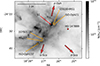 |
Fig. 1. Overview of the studied region. H2 column density map from Ladjelate et al. (2020) derived from Herschel data. Orange circles mark the location of the targeted sources and red stars mark the nearby massive stars HD147899 and S1. The red arrows point to the direction of the surrounding massive stars σ-Sco, α-Sco, and ρ-Oph, located at distances of ∼4.2–4.3, ∼4.3–5.2, and ∼2.3–3.1 pc from the protostars, respectively. |
The data were taken using the FASTR1 readout mode and a four-point dither pattern in the negative direction, optimized for extended sources. All three gratings (A, B, and C) were used thus covering the entire wavelength range available with MIRI(4.9–27.9 μm) with spectral resolution ranging from ∼0.0015 μm at 4.9 μm to ∼0.02 μm at 27.9 μm. A single pointing was used for each source targeting the corresponding source coordinates (see Table 1). The resulting field of view (FoV) depends on the MIRI Channel, and goes from 3.2″ × 3.7″ in Channel 1 (4.9–7.65 μm) up to 6.6″ × 7.7″ in Channel 4 (17.7–27.9 μm). The integration time per channel is also shown in Table 1. Two separate background observations were taken for sources in Oph A and Oph E and F, respectively.
The data were processed using the JWST pipeline (Bushouse et al. 2024) with the reference context jwst_1188.pmap of the JWST Calibration Reference Data System (CRDS; Greenfield & Miller 2016). The raw data were initially processed using the Detector1Pipeline set at default and next, the Spec2Pipeline was used to create the calibrated detector images. The corresponding background was then subtracted and the fringe flat as well as the residual fringe correction (Kavanagh et al. in prep.) were applied. Next, using the Vortex Imaging Processing package (Christiaens et al. 2023) an additional bad pixel map was created. The final datacubes were then created from the calibrated detector files by using the Spec3Pipeline, with the drizzle algorithm (Law et al. 2023), separately for each sub-band and MIRI/MRS Channel. Both the master background and the outlier rejection steps were switched off at this stage, while the wavelength calibration from Pontoppidan et al. (2024) was included in the data reduction.
3. Results
3.1. Spatial distribution of mid-IR line emission
The MIRI range covers a number of H2 lines from the ground-state vibrational level, that are excellent probes of outflows from low-mass protostars (e.g., Neufeld et al. 2009; Nisini et al. 2010b; Giannini et al. 2011). The morphology of H2 emission in various lines is a powerful tool to trace the interaction of the molecular jet with the surrounding envelope (e.g., Nisini et al. 2010a; Tappe et al. 2012). In this section, we compare the H2 emission with those of atomic and ionic species, and discuss the results in the context of previous studies.
Figure 2 shows continuum-subtracted H2 S(5) maps for four out of five sources in our sample, revealing their outflow characteristics. We detect two distinct outflow morphologies: (i) a narrow, collimated outflow structure (GSS30-IRS 1 and ISO-Oph 137), and (ii) a wide opening angle, butterfly-shaped outflow with extended outflow cavities ([GY92] 197 and WL 17). The remaining source, ISO-Oph 21, shows weak H2 emission in the S(1) and S(2) lines, has no clear outflow morphology, and no other transition is detected.
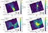 |
Fig. 2. Integrated emission of H2 S(5) line at 6.91 μm toward GSS30-IRS 1, ISO-Oph 137, [GY92] 197, and WL 17. The positions of the protostars, measured from the line-free region at 6.9 μm, are shown with black stars. The red arrows shows the apparent outflow direction based on the H2 emission. The filled black circle marks the spatial resolution of MIRI at λ = 6.9 μm (∼0.2″). |
Gaussian fitting velocity estimates for the warm and hot H2 gas components.
Apart from H2, several atoms and ions also show significantly extended line emission. Figure 3 shows the morphology of the most extended ionic emission in each source, namely that of the [Fe II] line at 5.34 μm for [GY92] 197 and ISO-Oph 137, the [Fe II] line at 25.9 μm for GSS30-IRS 1, and the [Ne II] line at 12.8 μm for WL 17. In the latter source, [Fe II] emission is not detected. The full list of detections, for every source and location, is given in Table A.1.
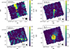 |
Fig. 3. Integrated emission of selected emission lines of ionized species: the [Fe II] line at 25.9 μm toward GSS30-IRS 1, the [Fe II] line at 5.34 μm toward ISO-Oph 137, and [GY92] 197, and – since no extended [Fe II] emission was detected – the [Ne II] line at 12.8 μm toward WL 17. The labels are the same as in Fig. 2. |
The ionic emission reveals well-collimated jets in GSS30-IRS 1, ISO Oph 137, and [GY92] 197. The jet of GSS30-IRS 1 is detected in multiple transitions of [Fe II], and shows a bipolar morphology extending in the North-South direction (Fig. 3). Because of the offset of Channel 4 relative to Channels 1-3 of MIRI, the southern lobe that is not visible in H2 can still be detected in the longer wavelength transitions of [Fe II]. In any case, the limited FoV of MIRI prevents the full extent of the outflow from being captured.
In ISO-Oph 137 and [GY92] 197, the [Fe II] emission tracing the jet is detected only toward one of the outflow lobes in each source (Fig. 3). Thus, the morphology differs from the emission seen in H2, which shows a bipolar symmetry (Fig. 2). Emission in additional ionic tracers, in particular [Ne II] at 12.8 μm, shows a compact morphology close to the protostar position of ISO-Oph 137, but an extended pattern in [GY92] 197. In WL 17, which shows a particularly wide opening angle in the H2 maps, no collimated jet is detected in atomic or ionic lines. In the following subsections, we discuss observations from MIRI/MRS in the context of previous studies of our sources from the literature.
3.1.1. GSS30-IRS 1:
The outflow activity in GSS30-IRS 1 was identified by the detection of extended line wings of CO (Tamura et al. 1990) and its association with a bright bipolar reflection nebula (Weintraub et al. 1993). The outflow morphology was subsequently studied with single dish CO J = 3 − 2 observations with a resolution of 14″ from the James Clerk Maxwell Telescope (JCMT) (White et al. 2015). Subsequent, high-resolution (∼0.6″) CO J = 2 − 1 observations from ALMA revealed a significant overlap of the blueshifted and redshifted outflow components of GSS30-IRS 1, suggesting a large inclination angle (Friesen et al. 2018). While MIRI observations of the H2 outflow are restricted to a single lobe, the spatial extent of [Fe II] confirms the N-S direction of the outflow (see Fig. 3). The disk inclination angle of i ∼ 60° from Michel et al. (2023) and Artur de la Villarmois et al. (2019) agrees with a scenario where the narrow collimated jet displays a well-separated bipolar morphology, and the CO emission shows a significant overlap between the outflow lobes.
3.1.2. ISO-Oph 137:
ISO-Oph 137 is host to a well-studied protoplanetary disk (Brandner et al. 2000; Pontoppidan et al. 2005; van Kempen et al. 2009); however, a corresponding molecular outflow has not been reported. The N-S orientation of the H2 outflow in the MIRI/MRS maps (see Fig. 2), along with a clear separation of the two outflow lobes, agrees with the proposed edge-on disk orientation (van Kempen et al. 2009). The collimated morphology of the outflow traces highly excited gas over a small volume, which could explain the lack of significant low-J CO emission.
3.1.3. [GY92] 197:
[GY92] 197 possesses a CO outflow that extends close to the plane of the sky in the E-W direction, revealed by low-J CO single-dish observations (at a resolution of 22 and 40″, respectively) by Bussmann et al. (2007) and Nakamura et al. (2011). The atomic and ionic emission from MIRI confirms the proposed outflow orientation (see Fig. 3) and is consistent with the almost vertical and edge-on disk (Michel et al. 2023). The H2 emission shows broad outflow cavities (Fig. 2), which are likely associated with the hourglass-shaped nebulosity detected in near-IR images (Duchêne et al. 2004).
3.1.4. WL 17:
WL 17 is a confirmed embedded YSO (van Kempen et al. 2009), which drives a bipolar outflow extending in a NW-SE direction as seen in single dish CO J = 3 − 2 observations (at a resolution of 15″, van der Marel et al. 2013). High-resolution ALMA observations (∼0.03″) revealed prominent cavities in both outflow lobes (Shoshi et al. 2024). Both the direction of the outflow and the presence of cavities are also seen in the MIRI/MRS H2 maps (Fig. 2). In this extended source, [Ne II] emission is seen, filling up the H2 cavity (bottom right panel in Fig. 3). Given the broad shape of the emission, the Ne II does not appear to be associated with any kind of jet launched from the protostar. Scattering of [Ne II] emission from the source onto the cavity walls offers a likely explanation for the wide morphology of the emission.
3.1.5. ISO-Oph 21:
The outflow of ISO-Oph 21 was identified via the blueshifted and redshifted line wings of CO, but the resolution was insufficient to study its morphology (White et al. 2015). The source was classified as a disk source, based on the distribution of dust continuum and dense gas emission, questioning its embedded nature (van Kempen et al. 2009). MIRI/MRS observations of ISO-Oph 21 show only very weak H2 emission in the lowest rotational levels and no atomic or ionic emission. Thus, we cannot confirm the presence of an outflow from this source. The apparent lack of an outflow in ISO-Oph 21 is potentially due to its more evolved stage (Table 1). The initial detection suffered from poor angular resolution, which could lead to the confusion with prominent outflows driven by nearby sources (see Fig. 9 in White et al. 2015).
3.2. Spectra
We used the information about the spatial distribution of the H2 emission to identify regions for the subsequent analysis. Namely, depending on the H2 emission patterns, we selected 3 to 8 circular apertures for each of the sources, making sure they lie within the FoV covered by the MRS spectrometer across the full MIRI wavelength range. The exact location of the apertures for each source are shown in Fig. E.12. The radius of the circular apertures is 0.5″, ensuring they cover a significant number of pixels in all four MIRI Channels. For sources with collimated outflows, we selected four (ISO-Oph 137) and three (GSS30-IRS 1) regions along the outflow direction, omitting the central region, which is strongly affected by extinction from the protostellar envelope. In case of WL 17 and [GY92] 197, characterized by the butterfly-shaped emission (Section 3.1), we selected 4 apertures in each of the outflow lobes, 8 for each object in total. In the case of ISO-Oph 21, where no clear outflow is detected, the aperture locations where selected to cover the area of the most prominent H2 emission.
3.2.1. Line detections across the maps
Several transitions of H2v = 0−0 are detected toward all targeted low-mass protostars in Ophiuchus (Table 1), except ISO-Oph 21, where only the S(1) and S(2) transitions are detected. None of the sources shows lines of H2v = 1−1, which were detected toward other low-mass protostars (e.g., Tychoniec et al. 2024). In addition, several atomic and ionic emission lines are present in the MIRI/MRS wavelength range. Among these, the most commonly detected lines are the [Fe II] lines at 5.34 μm (4 sources), the [S I] line at 25.2 μm (4 sources), and [Ne II] line at 12.8 μm (3 sources). A summary of the line emission detected in each aperture and each source is presented in Table A.1.
In GSS30-IRS 1, S(3) to S(8) H2 lines are detected along the full outflow extent, whereas the S(1) and S(2) lines are only detected in its outermost parts (Fig. 2). The reason for the non-detection of lowest-excited lines is due to an increase in the noise level in the spectra, likely resulting from the imperfect fringe correction due to the bright continuum emission toward the protostar’s position. It is worth noting that the [Ne II] line at 12.8 μm line is not detected toward GSS30-IRS 1, and the [S I] line at 25.2 μm is detected only in the outflow positions (B and C).
In ISO-Oph 137, S(1) to S(7) H2 lines are detected in all apertures, and the most highly excited S(8) line is also detected toward the B and D positions – at the tip of the outflow imaged with MIRI/MRS (Fig. 2). The non-detection of the S(8) line close to the protostar is most likely due to blending with the H2O and CO lines present in absorption toward the protostar position (Rocha et al., in prep.). Additionally, the [Fe II] lines are detected toward all positions except position A. The [Ne II] line at 12.8 μm and [S I] line at 25.2 μm are detected along the entire outflow.
In [GY92] 197, H2 lines up to S(8) are detected in the western outflow lobe, which shows a brighter H2 emission in general (Fig. 2). The lack of highly excited H2 lines in the bulk of the eastern outflow lobe, except the position closest to the protostar, is likely due to sensitivity limits of the observations. While [GY92] 197 is characterized by the largest number of detections of atomic and ionic species among all sources (Table A.1), such emission is absent in the eastern outflow lobe, except the [Ne II] line at 12.8 μm.
In WL 17, H2 lines up to S(8) are detected across all apertures. From the ionic and atomic emission lines, the [Ne II] line at 12.8 microns is the most prominent, being detected in all positions except position D. In contrast, [Fe II] is only seen in aperture E, close to the location of the protostar.
In ISO-Oph 21, the lack of emission from H2 transitions above S(2) is consistent with the lack of a clear outflow morphology (Section 3.1). It also lacks any emission from atomic and ionic lines due to the absence of a jet.
3.2.2. Gas kinematics
Jets from protostars are often characterized by gas velocities exceeding 100 km s−1, primarily seen in atomic and ionic lines (Frank et al. 2014; Bally 2016). Observations with MIRI, with a velocity resolution from ∼85 (in MIRI/MRS Channel 1) to ∼200 km s−1 (in Channel 4), may provide some information about the gas kinematics. For instance, a fast-moving jet resulting in velocity shifts of molecular and atomic mid-IR lines was reported in HH46 (Nisini et al. 2024).
We investigated the line profiles of molecular and ionic lines to search for possible velocity shifts across the maps. We focused on apertures corresponding to the location of H2 jets (Fig. 2) to maximize the chance to detect any velocity gradients.
Figure 4 shows the results obtained for WL 17, the only source in the sample where velocity shifts can be noticed in the [Ne II] line at 12.8 μm. However, similar shifts are not as clear in the H2 lines toward this source. It is worth noting that WL 17 does not possess a collimated H2 jet, and is characterized by a wide opening angle in molecular emission, and a rather compact pattern of ionic emission (Figs. 2, 3). We note here that the one sided detection of ionic emission in ISO-Oph 137 and [GY92] 197 restricts our ability to compare the velocities between the two lobes of the jet, where differences in velocity would be most prominent. Additionally, the incomplete coverage of the GSS30-IRS 1 outflow, where only one lobe is covered in all wavelengths makes such a comparison impossible in its case.
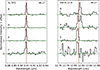 |
Fig. 4. Continuum-subtracted spectra of H2 S(5) (left) and [Ne II] 12.8 μm (right) toward WL 17. An offset is added to the spectra at various positions on the maps for better visualization. The dashed lines show the laboratory wavelengths of the respective transitions. |
We also estimated gas velocities of the different H2 transitions, using Gaussian fits to the spectra of each source and from each aperture. This approach, when applied to sufficiently strong lines, enables us to estimate velocity shifts at a resolution better than the instrumental MIRI/MRS resolution. Table 2 shows the resulting velocities for a warm gas component, estimated as the average velocity of the S(2) and S(3) transitions, and the velocity of the only the S(7) transition for a hot component. The presence of two separate gas components, warm and hot, respectively, is established through the rotational diagram analysis in Sect. 4. Here, we selected these transitions as they represent the best detected lines associated with the warm and hot components, respectively. In most cases, despite the similar spatial distribution of the two components, the hot component displays somewhat higher velocities than the warm component, potentially indicating that the hot component has a stronger connection to the fast moving jet. Similar to the direct spectral comparison, the hot component of WL 17 is the only case in which a noticeable velocity shift between the two lobes can be seen. We detect redshifted emission in the northern lobe and blueshifted toward the south, matching the orientation of the entrained CO outflow (Shoshi et al. 2024). Still, velocities for all H2 lines lie within a single spectral channel of MIRI/MRS indicating that the molecular gas component of the protostellar ejections is associated with material moving at lower velocities than the dominant atomic and ionized gas components (Harsono et al. 2023; Tychoniec et al. 2024).
4. Analysis
MIRI/MRS imaging of H2 emission on 100 AU scales allows us to associate molecular gas with the outflows from Class I protostars. Detection of multiple H2 lines can constrain both the gas excitation as well as the shock properties responsible for the emission. However, external UV radiation in the Ophiuchus region likely also influences the shock structure and its observational signatures. In the following sections, the gas excitation toward four protostars in Ophiuchus and its spatial variation are discussed (Section 4.1), and the ratios of selected H2 lines are compared with the predictions of shock models including the effects of external UV radiation (Section 4.2).
4.1. Rotational diagrams of H2
Rotational diagrams are commonly used to estimate gas physical conditions and column densities of molecules along outflows from low-mass protostars (e.g., Neufeld et al. 2009; Herczeg et al. 2012; Karska et al. 2013; Green et al. 2016; Manoj et al. 2013; Yang et al. 2018). The detection of multiple H2 lines with MIRI/MRS (Section 3.2) allows the determination of the gas rotational temperatures and the corresponding H2 column densities across the maps of protostars in Ophiuchus.
For optically thin, thermalized lines, the natural logarithm of the column density of the upper level, Nu, of a given transition over its degeneracy, gu, is related linearly to the energy, Eu, of that level (Mangum & Shirley 2015):
where Q(Trot) is the rotational partition function at a temperature, Trot, for a given molecule and Ntot is the total columndensity.
The level-specific column density, Nu, was calculated from the measured line intensities, Iul:
where Aul the Einstein emission coefficient, h the Planck constant, and ν the frequency of the line. The line intensities, following the approach presented in Francis et al. (2025), were calculated using the integrated fluxes (Ful; shown in Table B.1) as Iul = Ful/Ω, where Ω is the opening angle for an aperture with a diameter of 1″ at the distance of Ophiuchus (137 pc; Ortiz-León et al. 2017).
Due to significant dust content in the envelopes of low-mass protostars, mid-IR lines of H2 have to be corrected for extinction. We followed the procedure described in detail in Francis et al. (2025), in which the wavelength-dependent correction factor was determined from the fit to the rotational diagram using uncorrected intensities. Due to the positive curvature of our H2 rotational diagrams, we fit the natural logarithm of the column densities obtained from observations (Eq. (2)) over the level degeneracy, gu, with a two-temperature component fit and an additional term for the ortho-to-para ratio (OPR)correction:
![$$ \begin{aligned} y = \mathrm{ln} \left[ \left(N_{\rm warm}\frac{\mathrm{exp} (-E_\mathrm{u} /T_\mathrm{warm} )}{Q(T_\mathrm{warm} )} + N_\mathrm{hot} \frac{\mathrm{exp} (-E_\mathrm{u} /T_\mathrm{hot} )}{Q(T_\mathrm{hot} )}\right) 10^{\frac{-A_\lambda }{2.5}}\right] + z(J) ,\end{aligned} $$](/articles/aa/full_html/2025/11/aa54977-25/aa54977-25-eq3.gif)
where Aλ is taken from the KP5 extinctions curve (Pontoppidan et al. 2024), and with
where OPR is the ortho-to-para ratio. This way, we obtained the H2 column densities and temperatures of two gas components, as well as the value of the local extinction. In the two-component fit, the low and high temperature components are primarily constrained by the S(1)-S(4) and S(5)-S(8) transitions, respectively.
Figure 5 shows example rotational diagrams for each source in our sample, except ISO-Oph 21 (see Section 3), and for the aperture in which the number of H2 line detections was the largest. Table 3 shows the temperatures and column densities obtained for all sources and apertures.
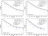 |
Fig. 5. H2 rotational diagrams for the outflow positions in WL 17, [GY92] 197, ISO-Oph 137, and GSS30-IRS 1 with the largest number of line detections. The natural logarithm of the column density from a level u, Nu, divided by the degeneracy of the level, gu, is written on the Y axis. The extinction-corrected values are shown in red, and the ones before the correction in blue. The two-component fits cover the transitions below and above Eu∼4000 K for the “warm” (dashed line) and “hot” (dotted line) component (see text). The combined fit is shown as a black line. Finally, letters next to source name mark the aperture where the H2 were measured. |
Rotational temperatures, column densities, extinction, and ortho-to-para ratios for all sources and apertures.
The H2 rotational diagrams are described well by the two components model with distinct temperatures, corresponding to Twarm of ∼500–600 K, and Thot of ∼1000–3000 K (Fig. 5). The warm component temperatures show a relatively narrow range considering also other apertures, whereas the range of the hot component values spans thousands of K (Table 3). It is worth noting that a small number of line detections corresponding to the hot component results in significant uncertainties of the fit. Similarly, the warm component of GSS30-IRS 1 in apertures A and B is also less constrained, and likely overestimated, due to the lack of detections of S(1)-S(2) lines caused by the strong continuum emission in the region (see Section 3.2). We find OPR = 2–3 for most cases, consistent the results of previous studies on the OPR within protostellar outflows (e.g., Neufeld et al. 2006). For GSS30-IRS 1 we adopt the equilibrium OPR ratio of 3 due to the non-detection of S(1) and S(2) lines, where the effects of deviation from the OPR = 3 are mostprominent.
The spatial variations in the rotational temperatures toward two sources with distinct morphologies are presented in Fig. 6. ISO-Oph 137 is a source with a bipolar collimated outflow that shows a clear increase in the gas temperatures toward the map edges – a trend that is confirmed by the detections of S(8) lines only toward the outermost apertures (Table A.1). Such a morphology is consistent with the presence of “shock spots” tracing the interaction of the jet and/or outflow with the surroundings, seen for example in L1157 (Nisini et al. 2010a). [GY92] 197, on the other hand, drives an outflow with a wide opening angle, and shows significantly less variation in the gas temperatures (Fig. 6). The western outflow lobe, which shows brighter H2 emission, seems to be associated with warmer gas than the eastern outflow lobe. Generally, the highest temperatures correspond well with the positions along the outflow cavity rather than the ionic jet. This is seen also in the eastern outflow lobe, where one of the positions is associated with especially high hot component (aperture H). The higher rotational temperatures found along the edges of the outflow cavity suggest that the H2 is heated by shocks produced at the cavity walls instead of along the central jet. Such shocks likely arise from the interaction between the outflowing gas and the surrounding cold envelope.
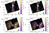 |
Fig. 6. Integrated emission of H2 S(5) line toward ISO-Oph 137 (top) and [GY92] 197 (bottom) with circles color-coded with the rotational temperatures of warm (left) and hot (right) gas components, respectively. Red arrows show the outflow directions, and capital letters refer to apertures used for the spectra extraction. |
The variation in gas excitation at different positions along the outflows is further explored in Fig. 7. Here, we calculate the ratio of two H2 transitions that are detected toward most of our sources: the S(2) line from the warm gas component and the S(7) line from the hot gas component (see also Section 4.2). The median ratio for our sources is ∼1.0. The highest values of the ratio correspond to the central positions of the ISO-Oph 137, which show significantly lower excitation than the outermost parts of the outflow (see Fig. 6). Overall, the S(2)/S(7) ratio for the Ophiuchus protostars, constituting only Class I protostars, is about a factor of 3 higher than the same ratio calculated for other low-mass protostars using the literature data (Tychoniec et al. 2024; Francis et al. 2025). We discuss a possible impact of evolutionary trends on the H2 excitation inSection 5.
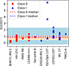 |
Fig. 7. Ratio of the S(2)/S(7) H2 emission lines in different low-mass protostellar sources. Red points mark Class 0 sources from Francis et al. (2025) and blue points are Class I sources from this work and TMC1-E from Tychoniec et al. (2024). The dashed lines mark the median values, 0.3 for Class 0 (in red) and 1.0 (in blue). Colored areas mark the median ± standard deviation range. |
To summarize, the analysis of H2 lines confirms the presence of highly excited molecular gas with properties showing some changes depending on the exact origin of the emission; for example, along the outflow cavities or jet. The differences between sources in our sample are not significant, suggesting that neither the source properties nor environmental conditions play a strong role in the H2 excitation.
4.2. Comparisons to shock models
In this section, we compare the measured H2 intensities from our observations to the results of models of UV-irradiated shocks propagating in a broad range of physical conditions of the ISM (Kristensen et al. 2023). We aim to constrain the shock properties for the Ophiuchus protostars and identify the impact of external UV radiation from nearby B-type stars on the H2 excitation in their outflows.
The model grid from Kristensen et al. (2023) was obtained using the Paris-Durham3 shock code that simulates the changes in the chemical, thermal and dynamical conditions of interstellar matter due to steady state, plane parallel shocks (Flower & Pineau des Forêts 2003). In its latest version, the code accounts for the impact of external UV irradiation on the shock structure and chemistry (Lesaffre et al. 2013; Godard et al. 2019).
Kristensen et al. (2023) considers the following input parameters of the environment and shock properties: (i) the pre-shock gas density nH, (ii) the traverse magnetic field strength,  in units of μGauss, where b is a scaling factor for magnetic field, (iii) the shock velocity vsh (iv) the external UV radiation field in units of G0, (v) the cosmic ray ionization rate ζH2, and (vi) the abundance of polycyclic aromatic hydrocarbons, X(PAH). The code calculates a chemical steady-state for a given gas density, nH, and UV field (step 1), the chemical equilibrium results are used as input for a PDR calculation (step 2), and the resulting PDR conditions are used as inputs for the shock model (step 3), for details see Section 2 of Kristensen et al. (2023). The excitation of H2 is subsequently calculated, taking into considerations collisions with H (Flower 1997; Flower & Roueff 1998; Martin & Mandy 1995), H2 (Flower & Roueff 1998), and He (Flower et al. 1998). The resulting H2 line intensities, along with a number of atomic line intensities, are provided in a machine-readable format on CDS4.
The shock model predictions from Kristensen et al. (2023) are provided for the following ranges of parameters: nH from 102 to 108 cm−3, b from 0.1 to 10, vsh from 2 to 90 km s−1, G0 from 0 to 103, ζH2 from 10−17 to 10−15 s−1, and X(PAH) from 10−8 to 10−6. Here, we restrict the considered parameters to those expected in outflows from low-mass protostars. In particular, typical (post-shock) gas densities in outflows are in the range from 105–108 cm−3 (Mottram et al. 2014), given the high compression factors predicted in Kristensen et al. (2023) all available pre-shock densities, from 102–106 cm−3 are considered. For such densities, the b scaling factor of 0.1–1 provide magnetic field strengths of the order of 0.001–1 mG, consistent with the recent measurements for the Ophiuchus molecular cloud (Lê et al. 2024). The shock velocities above 10 km s−1 are expected based on the resolved profiles of H2O and high-J CO lines with Herschel (Kristensen et al. 2012, 2017). Since the line profiles are not resolved with MIRI, the maximum shock velocities are ∼60 km s−1, but more likely they are not exceeding ∼30 km s−1 if they trace a similar gas component as H2O. The ionization by cosmic rays and PAH abundances are not known for the studied region in Ophiuchus; however, neither of these parameters have a significant impact on our analysis (Appendix H5). Here, we adopt the values from the low-end of the grid, ζ = 10−17 s−1 and X(PAH) = 10−7.
Figure 8 shows the comparison of the shock model results with the S(2)/S(7) ratios measured in the outflows from Ophiuchus protostars (see Section 3). Depending on the assumed magnetic field strength, the S(2)/S(7) ratio shows significant differences for a given value of pre-shock density but varying UV fields. Here, we consider magnetic fields with b = 0.1, representative of predominantly dissociative J-type shocks where ionic and neutral fluids are well coupled (Neufeld & Dalgarno 1989; Flower & Pineau Des Forêts 2010), and b = 1, typically adopted for C-type shocks, where ions and neutrals are decoupled (Kaufman & Neufeld 1996; Flower & Pineau Des Forêts 2010).
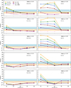 |
Fig. 8. Ratio of the S(2) over the S(7) transition of H2 against the shock velocity for different UV field strengths. The log(nH) ranges from 2 to 6 from top to bottom, while magnetic field strength is b = 0.1 for the left column and 1 for the right. For all panels ζ = 10−17 s−1, and X(PAH) = 10−7 are used. The shaded blue region marks the observed range of S(2)/S(7) ratios for the sources in Ophiuchus, while the beige region marks the range for Class 0 sources from Francis et al. (2025). Note that line intensities from Kristensen et al. (2023) are not available for all combinations of model parameters covered in the figure. |
The behavior of the S(2)/S(7) line ratio is notably different between the two types of shocks. For the lower density scenarios (nH = 102 − 103 cm−3) J-type shocks appear capable to reproduce the observed line ratios for a range of relatively low shock velocities (vsh = 10 − 20 km s−1), which becomes smaller for higher pre-shock densities and is already below 15 km s−1 at nH = 103 cm−3. The models also require an external UV field strength in the range of 1–100 G0 to match the observed line ratios. We note here that the external UV radiation field is either contributed to by the nearby stars or produced in accretion shocks and the radiation is escaping through the outflow cavity; the self-irradiation is negligible in such low-velocity shocks (Kristensen et al. 2023). For the same range of densities, C-type shocks only agree with the observed line ratios for a limited range of higher shock velocities (vsh = 20–25 km s−1). An exception to this limited velocity range is the case with nH = 103 cm−3 and UV field of 100 G0, which reproduces the observed ratios for vsh = 10–25 km s−1. The restricted velocity range in which C shocks are capable of reproducing the observed line ratios suggests that for pre-shock densities of nH = 102 − 103 cm−3J shocks are more likely responsible for the excitation of H2.
At pre-shock densities above 104 cm−3, the model S(2)/S(7) ratios for the J-type shocks decrease and span less than 2 orders of magnitude, and are generally not consistent with the ratios observed in the Ophiuchus sources. The only exceptions are the models assuming nH = 104 cm−3 and a complete absence of UV irradiation, or models with UV fields of 103 G0, which are too high for most low-mass star-forming regions (Karska et al. 2018; Kristensen et al. 2017; van Dishoeck et al. 2011). In contrast, the model ratios for the C-type shocks span several orders of magnitude and reproduce the observations for an extended range of shock velocities (vsh = 10–25 km s−1). At the pre-shock density of 104 cm−3, the S(2)/S(7) ratio decreases roughly by an order of magnitude with increasing values of UV field strengths. At the same time, the ratio does not depend strongly on the assumed shock velocity, facilitating meaningful comparisons with observations. For shock velocities in a broad range of values, from 10 to 20 km s−1, the best-fit value of G0 is 10–100. Slightly higher velocities would be also consistent with lower UV fields, but already at 25 km s−1 none of the models would reproduce the observations; thus, lower UV fields arerather unlikely.
At the pre-shock densities of 105–106 cm−3, the model ratios for C-type shocks decrease strongly with the increasing UV field strength and shock velocity (right column, middle and bottom panels of Fig. 8). At 15 km s−1, the best fit models suggest G0 of 1–10 for the pre-shock density of 105 cm−3, and G0 of 0 (a fully shielded scenario) for 106 cm−3. It is worth noting that G0 of 100 is also consistent with observations for faster shocks (vsh of 25–30 km s−1) at those higher pre-shock densities.
The sample of Class 0 sources from Francis et al. (2025) displays lower values for the observed S(2)/S(7) line ratios, suggesting higher excitation conditions within their outflows. The lower line ratios mean that the low-density, low-velocity J-type shocks require even higher values of UV irradiation (10–100 G0) in order to reproduce the observations. In addition, both higher pre-shock density (up to 104 cm−3) J- shocks with low velocities, as well as, high-velocity (vsh ≥ 20 km s−1), high-density nH ≥ 104 cm−3 solutions with UV fields of 100–1000 G0 are compatible with Class 0 sources.
In Appendix H5, we show that the choice of other H2 lines representing the warm and hot gas components does not significantly change the shock conditions required to reproduce the observations. We have also investigated various pairs of lines located either in the warm or in the hot component, but these ratios do not constrain well the shock models. A similar trend was noted with CO, where a broad range of shock conditions fit the observations of the warm component alone (Dionatos et al. 2013; Karska et al. 2013), whereas the inclusion of the external UV-irradiation of C-shocks allowed the curvature seen in rotational diagrams to be explained (Karska et al. 2018).
The shock model results presented in Kristensen et al. (2023) allow also for the reconstruction of full rotational diagrams, offering an alternate approach of comparing them to observations. Figure 9 shows a comparison between the rotational diagrams for two of the best models along with the extinction corrected rotational diagram from aperture A of WL 17 (see also Fig. 5), as an example among our observed rotational diagrams. The first model corresponds to a C-type shock with a pre-shock density of nH = 104 cm−3 that best reproduces the S(2)/S(7) ratio. The second model corresponds to a J-type shock with a pre-shock density of nH = 103 cm−3 that, in turn, best reproduces the two components rotational temperatures fit of the observations. Despite the C-shock model closely matching the observed S(2)/S(7) line ratio, in the range of velocities studied (10 km s−1 < vsh < 30 km s−1), it fails to reproduce the curvature seen in the rotational diagrams of our observations. Instead, it is best described by a single temperature component with Trot ∼ 900 K, a value that lies between that of the two components found in our observations. The J-shock model on the other hand, is best described by a two components fit, with Twarm ∼ 680 K and Thot ∼ 2000 K, values similar to those measured in our sample, and also displays the shift between the two components at a similar Eup. Despite better predicting the shape of the rotational diagram, model 2 predicts column densities of Nhot = 6.4 × 1016 cm−2 and Nwarm = 9.7 × 1017 cm−2, which are consistently one to two orders of magnitude lower than the values estimated for our Ophiuchus sources (see Table 3). In contrast, model 1 predicts Ntot = 2.8 × 1019 cm−2, in line with the observed values. We note here though that column densities predicted in shock models depend heavily on the assumed geometry of the shocks. Since models in Kristensen et al. (2023) assume a simple planar shock morphology whereas real shocks have complex morphologies, the reported differences in column densities are not sufficient to dismiss J-shocks. Overall, while comparing the full rotational diagram produced by different shock models to the observations has the benefit of considering all the information from the available transitions, it comes with some significant caveats in terms of the column densities and total fluxes, which rely on the assumed shock sizes and area.
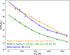 |
Fig. 9. Synthetic rotational diagrams based on the H2 intensities predicted for different combinations of parameters in the Kristensen et al. (2023) shock models. Green triangles show model results for nH = 103 cm−3, G0 = 100, vsh = 15 km s−1, b = 0.1, ζ = 10−17 s−1, and X(PAH) = 10−7. Orange diamonds show the model with nH = 104 cm−3, G0 = 100, vsh = 15 km s−1, b = 1, ζ = 10−17 s−1, and X(PAH) = 10−7. Blue points correspond to the observed values for aperture A of WL 17. Solid lines represent the best fit in each case. |
To summarize, H2 observations of outflows from four Class I protostars in Ophiuchus and five Class 0 sources studied by Francis et al. (2025) are consistent with the line ratios in both C- and J-type shocks. For the examined range of shock velocities, J-type shocks are also better at reproducing the overall shape of rotational diagrams, although they seem to underpredict the total column densities. Regardless, both kinds of models show that external irradiation by UV fields of the order of 10–100 in G0 units is required to best match the observations. As a next step, we determine UV radiation using other indirect methods to verify the results from shock models.
4.3. The impact of irradiation environment on the protostars in Ophiuchus
To assess the strength of the external UV irradiation on the protostars in Ophiuchus, we considered two additional methods: (i) UV radiation from nearby stars, and (ii) emission from dust assuming that all UV radiation was absorbed and re-emitted in the far-IR. We followed the procedure from Schneider et al. (2016, 2023) to calculate the UV flux at the position of each of our sources and originating from young, massive stars in the region. We considered several nearby stars and/or binaries: σ-Sco, a B1 III and B1 V type binary (Maíz Apellániz et al. 2021); α-Sco, a M1.5 Iab and B2 V type binary (Maíz Apellániz et al. 2021); ρ-Oph, a B2 IV and B2 V type binary (Abt 2011); HD 147889, a B2 V type star (Chini 1981; Liseau et al. 1999); and S1 (GSS35), a B3 V type star (Wilking et al. 2005). The total UV luminosity emitted by each of those stars was calculated from

where r is the stellar radius and T is the effective temperature of the star. Values for the radius and effective temperature of each source are taken from Drilling & Landolt (2000), based on their spectral type. The integration between 910 and 2066 Å covers far-UV photons relevant for the star-forming regions, with energies between 6 and 13.6 eV.
To obtain the UV flux at the position of protostars, the total UV luminosity from nearby stars was scaled by a factor of (4πR2)−1, where R is the distance between the source of UV radiation and the respective target in Ophiuchus. Due to the high uncertainties of line-of-sight distances, we assumed all considered objects to be at the same distance from Earth, and thus used the projected distances for the calculation (Schneider et al. 2016, 2023). The distances between the B-type stars and the protostars range between ∼4.2–4.3 pc for σ-Sco, ∼4.3–5.2 pc for α-Sco, ∼2.3–3.1 pc for ρ-Oph, ∼0.6–1.3 pc for HD147899, and ∼0.1–0.9 pc for S1. The resulting UV fluxes for each of our sources are presented in Table 4. It is worth noting that this approach does not correct for dust attenuation, which is significant in dusty molecular clouds, and thus represents only an upper limit to the radiation reaching our protostars.
External UV field strengths in units of G0.
Perhaps a more accurate way to estimate the UV radiation field in the region is by using the far-IR dust emission. Under the assumption that the UV emission of nearby massive stars is fully absorbed and re-emitted in the far-IR, the local UV radiation field can be estimated from the total FIR intensity between 60 and 200 μm (Kramer et al. 2008; Roccatagliata et al. 2013; Schneider et al. 2016). Here, we use the Herschel/PACS continuum intensities at 70 and 160 μm, collected as part of the Herschel Gould Belt Survey (Ladjelate et al. 2020), to obtain an estimate of the far-IR intensity (IFIR). Then, the total UV field, in units of G0, is given by (Schneider et al. 2016)
Figure 10 shows the resulting map of the estimated FUV in the Ophiuchus where our targets are located. To obtain an estimate for each of our sources, we calculated the average FUV in a 12″ aperture around each protostar, corresponding to the resolution of the Herschel/PACS continuum (see Table 4).
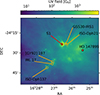 |
Fig. 10. Distribution of the interstellar UV radiation field estimated from the dust continuum emission from Herschel under the assumption that all UV radiation from nearby stars was absorbed and re-emitted in the far-IR. The G0 values presented here are likely overestimated due to contribution from thermal dust emission to the FIR continuum. Orange circles mark the location of the protostars, while red stars mark the position of the massive stars S1 and HD147899. α-Sco, σ-Sco, and ρ-Oph are located outside the FoV of this figure (similar to Fig. 1). |
The two methods presented above yield somewhat different results, with the general trend of the dust-based method predicting values higher by approximately a factor of 3, with the exception of ISO-Oph 21. Since the estimate from the nearby stars is expected to represent an upper limit of the FUV, the even higher values determined from the dust could be explained by the dust-based method accounting also for locally produced UV radiation, or from a significant contribution of thermal dust emission from the cloud (see also Schneider et al. 2016).
Both methods predict, however, that GSS30-IRS 1 stands apart from the other sources with a significantly higher FUV flux of the order of 103. ISO-Oph 21 has the second strongest FUV, with FUV ∼ 500 G0 based on the IFIR and ∼800 G0 based on the stellar emission. The remaining three sources show consistently similar UV fields of ∼300–400 G0 based on IFIR, and ∼100 G0 based on the stellar emission.
These results confirm the presence of significant variance in the UV conditions among protostars in Ophiuchus, allowing us to examine its potential impact on the star formation process. They are consistent with the estimates from UV-irradiated shock models implying UV fields of 10–100 times the average interstellar radiation fields.
5. Discussion
5.1. Origin of H2 emission in outflows from low-mass protostars
Mapping of pure rotational H2 lines with ISO and the InfraRed Spectrograph (IRS) on board Spitzer Space Telescope was a stepping stone to understand the molecular excitation in low-mass protostellar outflows (e.g., van Dishoeck 2004; Neufeld et al. 2006, 2009; Tappe et al. 2012). The low-J (J < 4) H2 emission in the prototypical outflow L1157 was associated with the wider cold molecular outflow traced by CO, while that of higher-J (J > 7) lines was connected to the precessing jet and more localized shocked regions (Nisini et al. 2010b). On the contrary, the morphology of outflows seen in various H2 transitions was rather similar (Giannini et al. 2011). Such a pattern resembles also our observations of low-mass protostars in Ophiuchus, where only slight variations in extent and opening angles are seen over different transitions even at the much smaller scales probed with JWST (see Section 3.1 and also Fig. G.16).
Detection of several H2 transitions allowed the determination of excitation temperatures of the emitting gas, accounting also for the nonequilibrium H2 ortho-to-para ratios (Neufeld & Yuan 2008; Neufeld et al. 2009). For an assumed power-law distribution of gas temperatures, with the column densities of material at temperature T to T + dT proportional to T−βdT, the best-fit power-law indices were found in the range 3.8–4.2 toward BHR71, L1448, and NGC 2071 (Giannini et al. 2011). The range of indices of 3.9–5.4 in L1157 indicated a large variation in the physical parameters along the outflows (Nisini et al. 2010b), in line with MIRI maps covering smaller spatial scales (Fig. 6).
Nisini et al. (2010b) and Giannini et al. (2011) also provide temperature estimates for selected locations along the outflows based on linear fits to the S(0)-S(2) and S(5)-S(7) lines, corresponding to a warm and hot gas component, respectively. The resulting values of Twarm ∼ 240–400 K and Thot ∼ 1000–1500 K are lower than the ones estimated in this work: 540 ± 70 K and 2000 ± 700 K for warm and hot component, respectively (Section 4.1). However, the difference in temperature could be due to the inclusion of the S(0) line and the lack of detections of higher-J lines due to limited sensitivity of Spitzer.
Important insights into the origin of hot molecular gas were enabled by Herschel, and the detection of high-J CO lines up to J = 48 and at a resolution of 9.4″, even toward outflows from low-mass protostars (Herczeg et al. 2012). Similar to H2, CO rotational diagrams revealed two dominant gas physical components with surprisingly similar temperatures of the warm component of ∼300 K toward all low-mass protostars (Karska et al. 2013; Green et al. 2013; Manoj et al. 2013). This gas temperature is consistent with the Spitzer results, but about 200 K lower than the respective warm component seen in H2 with MIRI (Section 4.1).
To investigate possible changes of gas temperature as the protostar evolves, Figure 11 shows a comparison of rotational temperatures of H2 and CO toward Class 0 and I objects. The H2 results for Class 0 objects are adopted from a recent study of on-source positions of five objects by Francis et al. (2025), whereas Class I temperatures refer to outflows from Ophiuchus protostars (Section 4), and a single source in Taurus – TMC1 (Tychoniec et al. 2024). The distribution of rotational temperatures based on CO and for Class 0 and I objects are adopted from a consistent analysis of ∼90 protostars with Herschel/PACS (Karska et al. 2018).
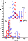 |
Fig. 11. Distribution of the rotational temperatures of H2 (top) and high-J CO (bottom) in low-mass protostars. Temperatures in Class 0 protostars are shown in red, and in Class I sources in blue. The warm gas component is shown in stripped bins, and the hot one in clear bins. H2 results for Class 0 protostars are adopted from Francis et al. (2025), and CO results for both Class 0 and I are from Karska et al. (2018). |
We find that the distribution of Twarm and Thot using H2 is tentatively shifted toward higher values for less evolved protostars (top panel of Fig. 11). However, the range of the hot component temperature is relatively broad for both Class 0 and I objects, reaching values of up to 3000 K. The difference is reflected by the average H2 rotational temperatures for the Class 0 objects of 660 ± 100 K (warm) and 2200 ± 600 K (hot) versus for the Class I objects of 520 ± 70 K (warm) and 1800 ± 550 K (hot).
Similar trend of decreasing rotational temperature with the evolutionary stage was not present using CO observations (bottom panel of Fig. 11). It is worth noting that the maximum temperatures obtained with CO did not exceed ∼1100 K, and the distribution of the hot component temperatures with Herschel of 760 ± 170 K (Karska et al. 2018) suggests that high-J CO lines might trace a less energetic part of the flow than H2.
A combined analysis of H2O and CO from Herschel provided solid evidence that both gas temperature components discussed above originate in non-dissociative shocks, with the hot component additionally tracing regions irradiated by UV radiation (Karska et al. 2014a, 2018; Kristensen et al. 2017). The impact of far-UV photons was further confirmed by high abundances of OH and other hydrides in the immediate surrounding of both low- and high-mas protostars (Wampfler et al. 2013; Benz et al. 2016). The H2 line ratios measured toward Ophiuchus protostars, favor the origin of H2 emission in the UV-irradiated shocks (Section 4.2). The ratio of the S(2)/S(7) lines for Class 0 objects is at the lower end of values for Class I objects (Fig. 7), which would imply higher UV-fields in those sources assuming the same gas densities (Fig. 8). Consequently, gas temperatures would be higher for Class 0 objects, consistent with the results of our rotational analysis (Fig. 11). However, the densities of the envelopes of Class 0 objects are typically higher than for Class I objects (e.g., Kristensen et al. 2012), which should reduce the impact of external UV radiation, in particular for the outflow positions closer to the central source. The small variation in excitation conditions among the Oph sources despite the significant difference of the UV field strength from the surrounding environment, as estimated in Sect. 4.3, suggests that the environmental UV radiation has little to no effect on the excitation within protostellar outflows. We note though that the positions examined in this work are located very close to the protostars, and therefore likely to be well shielded from the external UV radiation. In addition, some UV radiation can be also produced in-situ by the shock itself, but velocities above 30 km s−1, higher than measured using velocity-resolved H2O lines for low-mass protostars, would be required (Lehmann et al. 2020, 2022; Kristensen et al. 2023). Hence, accretion shocks and high velocity shocks along the protostellar jets are more likely sources for the UV radiation required to reproduce the excitation conditions observed in the Oph sources. Such an origin for the UV radiation also aligns with the slightly higher excitation conditions seen in Class 0 sources, since they are in general believed to have higher accretion rates and drive more powerful jets. Prompt OH emission, shown to probe well the UV field within protostellar outflows (e.g., Neufeld et al. 2024), could serve as an independent approach to confirm such evolutionary trends. Regardless, observations of larger number of sources with additional line tracers are needed to confirm the trend of higher gas temperatures in Class 0 objects and its interpretation.
In addition to the evolutionary stage, source properties such as the bolometric luminosity or envelope mass have also been closely associated with outflow properties (e.g., Cabrit & Bertout 1992; Yıldız et al. 2015; Mottram et al. 2017; Skretas & Kristensen 2022). To explore whether the observed shifts in temperatures and excitation conditions are associated with source properties, instead of the evolutionary stage of the sources, we look into the comparison of the warm component temperature over the bolometric luminosity of the source, for the same sample that was used in Figs. 7 and 11. Even though the sample is small, Fig. 12 shows no clear correlation between the source properties and the resulting H2 temperatures. In contrast, the slight shift between the Class I and Class 0 sources, initially noted in Fig. 11, is apparent. The lack of impact of the source properties on the excitation conditions within the outflows are further supported by the remarkable similarity of temperatures between low- and high-mass sources reported in Francis et al. (2025).
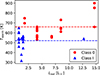 |
Fig. 12. Temperature of the warm gas component along the protostellar outflows over the bolometric luminosity of the corresponding driving source. Blue triangles show the Class I sources from this work and Tychoniec et al. (2024), while red circles show the Class 0 sample from Francis et al. (2025). Dashed blue and red lines show the mean values for the Class I and 0 sources, respectively. |
To summarize, H2 emission from protostellar outflows in Ophiuchus likely originates in shocks irradiated by UV fields produced in shocks along the protostellar jets or by accretion onto the protostar. By comparisons with other protostars observed with JWST (Francis et al. 2025), we find a trend of decreasing H2 rotational temperatures from Class 0 to Class I objects. In addition, we find no clear connection between the driving source properties and the excitation conditions within their outflows. The upcoming analysis of larger samples of protostars with JWST will certainly allow us to draw more solid conclusions on the origin of H2 emission.
5.2. Gas energetics in outflow shocks
Theoretical studies of line cooling from dense cores predict that most of the released energy is emitted in mid-IR emission from H2, followed by far-IR lines fines structure lines of [O I], high-J CO, and H2O rotational transitions (Goldsmith & Langer 1978; Takahashi et al. 1983; Neufeld & Kaufman 1993; Ceccarelli et al. 1996; Doty & Neufeld 1997). Similarly, H2 emission is the most significant cooling pathway for shock excited gas in protostellar outflows (Kaufman & Neufeld 1996; Flower & Pineau Des Forêts 2010; Kristensen et al. 2023). Thus, JWST observations of H2 lines allow us to study the energetics of protostars, at spatial scales significantly smaller than previously achieved with Spitzer (e.g., Nisini et al. 2010b; Giannini et al. 2011).
For a non-dissociative shock propagating in a medium with a pre-shock density of nH ∼ 104 cm−3 and vsh ∼ 10 − 50 km s−1, H2 luminosity corresponds to ∼20–70% of the total outflow cooling rate Kaufman & Neufeld (1996). This allows for the calculation of the total kinetic luminosity (Lkin) of the outflow from the observed rotational lines of H2 (Maret et al. 2009):
where (1 − fm) is the fraction of shock mechanical energy that is converted into internal excitation and fc is the fraction of cooling attributed to the H2 emission. In turn, the outflow mass rate can be calculated as
Adopting fc = 0.25–0.5, (1 − fm) = 0.75, and vsh ∼ 15–35 km s−1, Maret et al. (2009) report mass loss rates of the order of 10−6 M⊙ yr−1 for five Class 0 sources in NGC 1333 in Perseus.
We calculated the mass loss rate for the four outflow sources in Ophiuchus, by summing up the H2 line intensity measured in all the apertures (see Table C.1). In addition, we adopted fc= 0.5 and (1 − fm) = 0.75, similar to Maret et al. (2009), and assumed vsh = 15 km s−1, which best matches our observations (see Section 4.2). We find values of Ṁ ∼ 4–7 × 10⁻⁹ M⊙ yr−1, except for GSS30-IRS 1, where Ṁ = 2.8 × 10⁻⁸ M⊙ yr−1. The significantly higher value measured for GSS30-IRS 1 reflects the much stronger H2 emission compared to the rest of the sources, and could be partly due to inclusion of the extended and bright protostellar envelope in some of the apertures (Table 5).
Mass outflow rates and kinetic luminosities.
It is worth noting that the values estimated here represent lower limits for the true Ṁ values for our outflows due to the limited FoV of MIRI. The mass loss rates of ∼7.8 × 10⁻⁷ M⊙ yr−1 were obtained using low-J CO lines for the entire outflow from [GY92] 197 (van der Marel et al. 2013), so almost 2 orders of magnitude higher than the JWST estimates. However, those CO observations trace the entrained outflow gas, not the shocked gas inside the cavity seen in H2. Nevertheless, Nisini et al. (2010b) found a good agreement between the outflow parameters estimated from H2 and CO observations in L1157 (Bachiller et al. 2001), where the full extent of the outflow was considered. This study supported the scenario that the CO outflow is accelerated by the H2 flow; however, the angular resolution of existing CO observations for protostars in Ophiuchus is too low for similar comparisons.
An alternative calculation method proposed by Delabrosse et al. (2024) offers a more direct approach to estimate mass loss rates using the H2 lines within the MIRI range. For this method, the mass loss rate is given by

where mH is the hydrogen atom mass, NH2 the column density of H2, lperp the width of the molecular outflow, vrad the radial velocity of the flow, and i the inclination angle of the outflow. Table 6 shows the resulting mass loss rates for all sources, calculated separately for the warm and hot components of the outflows. The mass loss rates were calculated independently for each lobe and then summed to give the total rate for each source. For GSS30-IRS 1, where only one lobe is covered by our FoV, the given value corresponds only to the observed outflow lobe. We used the column densities derived from the rotational diagram analysis (Table 3). For the wide angle outflows of [GY92] 197 and WL 17, we used the average column density of the three apertures spanning the width of the outflow lobes (In both cases, apertures A, C, and D and E, G, and H, respectively, for each lobe). For GSS30-IRS 1, we used the values derived from aperture C due to the higher uncertainties in the cold component properties in apertures A and B, caused by the non-detection of the S(1) and S(2) lines due to the bright continuum (see Sect. 3.2). For ISO-Oph 137, we used the values from the apertures further away from the source (B and D) as the column densities derived for apertures A and C are likely overestimated. The radial velocities for each source were estimated from the Gaussian fitting (Table 2) and using the same apertures (or averages) as for the NH2. The width of the outflows (lperp) was measured directly from the integrated intensity maps, using the S(3) and S(7) transitions for the warm and hot components, respectively. Finally, for the inclination angle, we adopted the literature values of 60° for GSS30-IRS 1 (Artur de la Villarmois et al. 2019), and 34° for WL 17 (Shoshi et al. 2024), and for the edge-on disks of [GY92] 197 (Michel et al. 2023) and ISO-Oph 137 (van Kempen et al. 2009) we assumed i = 80°.
Overall, we find a broad range of mass loss rate among our sources, with values ranging from ∼10−7–10−9 M⊙ yr−1 for the warm and ∼10−9–10−11 M⊙ yr−1 for the hot component, respectively. Despite that fact that we only measure a single outflow lobe, the highest values are associated with the outflow of GSS30-IRS 1, the brightest source in our sample (see Table 1). Surprisingly, the outflow of [GY92] 197 also shows directly comparable mass loss rates, despite having an order of magnitude lower bolometric luminosity. In addition to that, the lowest mass loss rates we find are associated with ISO-Oph 137, a source with a comparable bolometric luminosity to that of [GY92] 197. This result may suggest that the morphology of the outflow, collimated or wide-angled, has an impact on the estimated outflow properties, with wide-angled outflows displaying higher outflow rates compared to collimated flows for sources with similar bolometric luminosities. Our sample though is extremely limited to draw any safe conclusions, and additional observations would be required to confirm or refute thissuggestion.
In addition, we find that the warm component carries most of the mass in the outflow, with mass loss rates approximately two orders of magnitude higher that those of the hot component. This difference directly reflects the two orders of magnitude difference seen in the column densities of the twocomponents. Comparing our results with previous works employing the same method we find that our results lie between the values estimated for the hot gas component of the Class I source DG Tau (Delabrosse et al. 2024) and those estimated for the Class 0 source HH211 (Caratti o Garatti et al. 2024). Namely, the mass loss rates for the hot component of ISO-Oph 137 (∼10−11 M⊙ yr−1) are directly comparable to the results of Delabrosse et al. (2024), while the mass loss rates for the warn component of GSS30-IRS 1 and [GY92] 197 (∼10−7 M⊙ yr−1) appear comparable to those of HH211. Finally, the mass loss rate for [GY92] 197, estimated using the “moving slab” method is also directly comparable to the low-J CO estimate of ∼7.8 × 10⁻⁷ M⊙ yr−1 (van der Marel et al. 2013). This results suggest that indeed, this method yields more accurate results, as it overcomes many of the limitations of the luminosity method discussed above. To summarize, our observations highlight the potential of JWST in constraining the energetics of outflows via the H2 emission.
6. Conclusions
In this work, we present JWST MIRI/MRS observations of 5 Class I protostars in the Ophiuchus molecular cloud. We analyze the H2 excitation associated with the protostellar outflows, and study the origin of the emission in shocks irradiated by external UV photons. The conclusions are as follows:
-
H2 outflows are detected in four out of five sources. These outflows display two distinct morphologies. Two of them appear narrow and well collimated (GSS30-IRS 1 and ISO-Oph 137), and the other two show wide opening angles with well-defined cavities (WL 17 and [GY92] 197).
-
Several atomic and ionic emission lines are detected, with the most common being those of [Ne II], [Fe II], and [S I]. Their emission is associated with narrow, well-collimated jets, even in cases in which the H2 emission traces outflow cavities.
-
The line emission along the outflows shows no significant velocity shifts between the outflow lobes, constraining the line-of-sight velocity of the H2 outflows to v < 90 km s−1. The only case in which a noticeable velocity shift is detected is the [Ne]II line at 12.8 μm in WL 17.
-
Rotational diagram analysis reveals that the H2 emission within the protostellar outflows is described well by a two-temperature-components model. The two components are found to have rotational temperatures in the range of Twarm ∼ 500–600 K and Thot ∼ 1000–3000 K.
-
Based on shock model results from Kristensen et al. (2023), the external UV irradiation is found to have a significant impact on the S(2)/S(7) H2 line ratios. By contrast, the cosmic ray ionization rate and PAH abundance appear to have minimal to no impact. The magnetic field strength seems to shift the observed behavior of the ratio to higher velocities, by allowing higher-velocity C-type shocks.
-
The observed S(2)/S(7) ratios agree with predictions from C-type shocks at pre-shock densities of nH ≥ 104 cm−3, as well as with low-density (nH ≤ 103 cm−3), low-velocity (vsh ≤ 15 km s−1) J-type shocks. The J-type shocks reproduce the observed positive curvature of the rotational diagrams better but at the same time underestimate the column densities.
-
The observations require the presence of substantial (∼10–100 G0) UV irradiation in shock models. The strength of the UV fields is higher than that derived for the nearby diffuse cloud (van Dishoeck & Black 1986), suggesting that some UV photons originate from the accretion shocks in protostellar systems.
Overall, our results present a detailed view of four different protostellar outflows at close distances from their driving source, highlighting their morphological differences and physical properties. The lack of substantial variation in outflow properties, despite the predicted variation in external UV field and model results, suggests that more work is still required, both to observationally constrain the UV field strength and also to accurately model its impact.
Data availability
Appendices D-H are available online on Zenodo.
The data used in this project may be obtained from https://doi.org/10.17909/g6cb-s335.
Appendix E is available online here.
Appendix H is available online here.
Appendix G is available online here.
Acknowledgments
We are grateful to Ewine F. van Dishoeck for useful insights and suggestions enhancing the overall quality of the manuscript. This work is based on observations made with the NASA/ESA/CSA James Webb Space Telescope. The data were obtained from the Mikulski Archive for Space Telescopes at the Space Telescope Science Institute, which is operated by the Association of Universities for Research in Astronomy, Inc., under NASA contract NAS 5-03127 for JWST. These observations are associated with program ID 1959. This publication is also based upon work from COST Action PLANETS CA22133, supported by COST (European Cooperation in Science and Technology). AK acknowledges support from the Polish National Science Center SONATA BIS grant No. 2024/54/E/ST9/00314. Astrochemistry in Leiden is supported by funding from the European Research Council (ERC) under the European Union’s Horizon 2020 research and innovation programme (grant agreement No. 101019751 MOLDISK), by the Netherlands Research School for Astronomy (NOVA), and by grant TOP-1 614.001.751 from the Dutch Research Council (NWO). MF acknowledges support from the Polish National Agency for Academic Exchange grant No. BPN/BEK/2023/1/00036/DEC/01 and from the Polish National Science Centre SONATA grant No. 2022/47/D/ST9/00419. The material is based upon work supported by NASA under award number 80GSFC24M0006 (M.S.).
References
- Abt, H. A. 2011, AJ, 141, 165 [NASA ADS] [CrossRef] [Google Scholar]
- Arce, H. G., Mardones, D., Corder, S. A., et al. 2013, ApJ, 774, 39 [CrossRef] [Google Scholar]
- Argyriou, I., Glasse, A., Law, D. R., et al. 2023, A&A, 675, A111 [NASA ADS] [CrossRef] [EDP Sciences] [Google Scholar]
- Artur de la Villarmois, E., Jørgensen, J. K., Kristensen, L. E., et al. 2019, A&A, 626, A71 [NASA ADS] [CrossRef] [EDP Sciences] [Google Scholar]
- Assani, K. D., Harsono, D., Ramsey, J. P., et al. 2024, A&A, 688, A26 [NASA ADS] [CrossRef] [EDP Sciences] [Google Scholar]
- Bachiller, R., Pérez Gutiérrez, M., Kumar, M. S. N., & Tafalla, M. 2001, A&A, 372, 899 [NASA ADS] [CrossRef] [EDP Sciences] [Google Scholar]
- Bai, X.-N., Ye, J., Goodman, J., & Yuan, F. 2016, ApJ, 818, 152 [Google Scholar]
- Bally, J. 2016, ARA&A, 54, 491 [Google Scholar]
- Benz, A. O., Bruderer, S., van Dishoeck, E. F., et al. 2016, A&A, 590, A105 [NASA ADS] [CrossRef] [EDP Sciences] [Google Scholar]
- Bontemps, S., André, P., Kaas, A. A., et al. 2001, A&A, 372, 173 [NASA ADS] [CrossRef] [EDP Sciences] [Google Scholar]
- Brandner, W., Sheppard, S., Zinnecker, H., et al. 2000, A&A, 364, L13 [NASA ADS] [Google Scholar]
- Bushouse, H., Eisenhamer, J., Dencheva, N., et al. 2024, JWST Calibration Pipeline [Google Scholar]
- Bussmann, R. S., Wong, T. W., Hedden, A. S., Kulesa, C. A., & Walker, C. K. 2007, ApJ, 657, L33 [Google Scholar]
- Cabrit, S., & Bertout, C. 1992, A&A, 261, 274 [Google Scholar]
- Caratti o Garatti, A., Ray, T. P., Kavanagh, P. J., et al. 2024, A&A, 691, A134 [NASA ADS] [CrossRef] [EDP Sciences] [Google Scholar]
- Ceccarelli, C., Hollenbach, D. J., & Tielens, A. G. G. M. 1996, ApJ, 471, 400 [Google Scholar]
- Chini, R. 1981, A&A, 99, 346 [NASA ADS] [Google Scholar]
- Christiaens, V., Gonzalez, C., Farkas, R., et al. 2023, J. Open Source Software, 8, 4774 [NASA ADS] [CrossRef] [Google Scholar]
- Delabrosse, V., Dougados, C., Cabrit, S., et al. 2024, A&A, 688, A173 [NASA ADS] [CrossRef] [EDP Sciences] [Google Scholar]
- Dionatos, O., Jørgensen, J. K., Green, J. D., et al. 2013, A&A, 558, A88 [NASA ADS] [CrossRef] [EDP Sciences] [Google Scholar]
- Doty, S. D., & Neufeld, D. A. 1997, ApJ, 489, 122 [NASA ADS] [CrossRef] [Google Scholar]
- Drilling, J. S., & Landolt, A. U. 2000, in Allen’s Astrophysical Quantities, ed. A. N. Cox, 381 [Google Scholar]
- Duchêne, G., Bouvier, J., Bontemps, S., André, P., & Motte, F. 2004, A&A, 427, 651 [NASA ADS] [CrossRef] [EDP Sciences] [Google Scholar]
- Enoch, M. L., Evans, N. J. I., Sargent, A. I., & Glenn, J. 2009, ApJ, 692, 973 [NASA ADS] [CrossRef] [Google Scholar]
- Evans, N. J. I., Dunham, M. M., Jørgensen, J. K., et al. 2009, ApJS, 181, 321 [NASA ADS] [CrossRef] [Google Scholar]
- Fall, S. M., Krumholz, M. R., & Matzner, C. D. 2010, ApJ, 710, L142 [NASA ADS] [CrossRef] [Google Scholar]
- Ferreira, J. 1997, A&A, 319, 340 [Google Scholar]
- Flower, D. R. 1997, MNRAS, 288, 627 [NASA ADS] [CrossRef] [Google Scholar]
- Flower, D. R., & Pineau des Forêts, G. 2003, MNRAS, 343, 390 [Google Scholar]
- Flower, D. R., & Pineau Des Forêts, G. 2010, MNRAS, 406, 1745 [NASA ADS] [Google Scholar]
- Flower, D. R., & Roueff, E. 1998, J. Phys. B At. Mol. Phys., 31, 2935 [NASA ADS] [CrossRef] [Google Scholar]
- Flower, D. R., Roueff, E., & Zeippen, C. J. 1998, J. Phys. B At. Mol. Phys., 31, 1105 [NASA ADS] [CrossRef] [Google Scholar]
- Francis, L., van Dishoeck, E. F., Caratti o Garatti, A., et al. 2025, A&A, 694, A174 [NASA ADS] [CrossRef] [EDP Sciences] [Google Scholar]
- Frank, A., Ray, T. P., Cabrit, S., et al. 2014, in Protostars and Planets VI, eds. H. Beuther, R. S. Klessen, C. P. Dullemond, & T. Henning, 451 [Google Scholar]
- Friesen, R. K., Pon, A., Bourke, T. L., et al. 2018, ApJ, 869, 158 [NASA ADS] [CrossRef] [Google Scholar]
- Giannini, T., Nisini, B., Neufeld, D., et al. 2011, ApJ, 738, 80 [CrossRef] [Google Scholar]
- Godard, B., Pineau des Forêts, G., Lesaffre, P., et al. 2019, A&A, 622, A100 [NASA ADS] [CrossRef] [EDP Sciences] [Google Scholar]
- Goldsmith, P. F., & Langer, W. D. 1978, ApJ, 222, 881 [Google Scholar]
- Green, J. D., Evans, N. J. I., Jørgensen, J. K., et al. 2013, ApJ, 770, 123 [NASA ADS] [CrossRef] [Google Scholar]
- Green, J. D., Yang, Y.-L., Evans, N. J. I., et al. 2016, AJ, 151, 75 [NASA ADS] [CrossRef] [Google Scholar]
- Greenfield, P., & Miller, T. 2016, Astron. Comput., 16, 41 [NASA ADS] [Google Scholar]
- Harsono, D., Bjerkeli, P., Ramsey, J. P., et al. 2023, ApJ, 951, L32 [NASA ADS] [CrossRef] [Google Scholar]
- Herczeg, G. J., Karska, A., Bruderer, S., et al. 2012, A&A, 540, A84 [NASA ADS] [CrossRef] [EDP Sciences] [Google Scholar]
- Karska, A., Herczeg, G. J., van Dishoeck, E. F., et al. 2013, A&A, 552, A141 [NASA ADS] [CrossRef] [EDP Sciences] [Google Scholar]
- Karska, A., Herpin, F., Bruderer, S., et al. 2014a, A&A, 562, A45 [NASA ADS] [CrossRef] [EDP Sciences] [Google Scholar]
- Karska, A., Kristensen, L. E., van Dishoeck, E. F., et al. 2014b, A&A, 572, A9 [NASA ADS] [CrossRef] [EDP Sciences] [Google Scholar]
- Karska, A., Kaufman, M. J., Kristensen, L. E., et al. 2018, ApJS, 235, 30 [NASA ADS] [CrossRef] [Google Scholar]
- Kaufman, M. J., & Neufeld, D. A. 1996, ApJ, 456, 611 [NASA ADS] [CrossRef] [Google Scholar]
- Kramer, C., Cubick, M., Röllig, M., et al. 2008, A&A, 477, 547 [NASA ADS] [CrossRef] [EDP Sciences] [Google Scholar]
- Kristensen, L. E., van Dishoeck, E. F., Bergin, E. A., et al. 2012, A&A, 542, A8 [NASA ADS] [CrossRef] [EDP Sciences] [Google Scholar]
- Kristensen, L. E., van Dishoeck, E. F., Mottram, J. C., et al. 2017, A&A, 605, A93 [CrossRef] [EDP Sciences] [Google Scholar]
- Kristensen, L. E., Godard, B., Guillard, P., Gusdorf, A., & Pineau des Forêts, G. 2023, A&A, 675, A86 [NASA ADS] [CrossRef] [EDP Sciences] [Google Scholar]
- Ladjelate, B., André, P., Könyves, V., et al. 2020, A&A, 638, A74 [NASA ADS] [CrossRef] [EDP Sciences] [Google Scholar]
- Law, D. R. E., Morrison, J., Argyriou, I., et al. 2023, AJ, 166, 45 [NASA ADS] [CrossRef] [Google Scholar]
- Le Gouellec, V. J. M., Maury, A. J., & Hull, C. L. H. 2023, A&A, 671, A167 [NASA ADS] [CrossRef] [EDP Sciences] [Google Scholar]
- Lê, N., Tram, L. N., Karska, A., et al. 2024, A&A, 690, A191 [NASA ADS] [CrossRef] [EDP Sciences] [Google Scholar]
- Lee, C.-F. 2020, A&A Rev., 28, 1 [NASA ADS] [CrossRef] [Google Scholar]
- Lehmann, A., Godard, B., Pineau des Forêts, G., & Falgarone, E. 2020, A&A, 643, A101 [EDP Sciences] [Google Scholar]
- Lehmann, A., Godard, B., Pineau des Forêts, G., Vidal-García, A., & Falgarone, E. 2022, A&A, 658, A165 [CrossRef] [EDP Sciences] [Google Scholar]
- Leous, J. A., Feigelson, E. D., Andre, P., & Montmerle, T. 1991, ApJ, 379, 683 [Google Scholar]
- Lesaffre, P., Pineau des Forêts, G., Godard, B., et al. 2013, A&A, 550, A106 [NASA ADS] [CrossRef] [EDP Sciences] [Google Scholar]
- Lindberg, J. E., Charnley, S. B., Jørgensen, J. K., Cordiner, M. A., & Bjerkeli, P. 2017, ApJ, 835, 3 [NASA ADS] [CrossRef] [Google Scholar]
- Liseau, R., White, G. J., Larsson, B., et al. 1999, A&A, 344, 342 [NASA ADS] [Google Scholar]
- Loren, R. B., Wootten, A., & Wilking, B. A. 1990, ApJ, 365, 269 [NASA ADS] [CrossRef] [Google Scholar]
- Maíz Apellániz, J., Barbá, R. H., Fariña, C., et al. 2021, A&A, 646, A11 [NASA ADS] [CrossRef] [EDP Sciences] [Google Scholar]
- Mangum, J. G., & Shirley, Y. L. 2015, PASP, 127, 266 [Google Scholar]
- Manoj, P., Watson, D. M., Neufeld, D. A., et al. 2013, ApJ, 763, 83 [NASA ADS] [CrossRef] [Google Scholar]
- Maret, S., Bergin, E. A., Neufeld, D. A., et al. 2009, ApJ, 698, 1244 [NASA ADS] [CrossRef] [Google Scholar]
- Martin, P. G., & Mandy, M. E. 1995, ApJ, 455, L89 [NASA ADS] [CrossRef] [Google Scholar]
- Melnick, G. J., & Kaufman, M. J. 2015, ApJ, 806, 227 [NASA ADS] [CrossRef] [Google Scholar]
- Michel, A., Sadavoy, S. I., Sheehan, P. D., et al. 2023, AJ, 166, 184 [NASA ADS] [CrossRef] [Google Scholar]
- Mirocha, A., Karska, A., Gronowski, M., et al. 2021, A&A, 656, A146 [NASA ADS] [CrossRef] [EDP Sciences] [Google Scholar]
- Motte, F., Andre, P., & Neri, R. 1998, A&A, 336, 150 [NASA ADS] [Google Scholar]
- Mottram, J. C., Kristensen, L. E., van Dishoeck, E. F., et al. 2014, A&A, 572, A21 [NASA ADS] [CrossRef] [EDP Sciences] [Google Scholar]
- Mottram, J. C., van Dishoeck, E. F., Kristensen, L. E., et al. 2017, A&A, 600, A99 [NASA ADS] [CrossRef] [EDP Sciences] [Google Scholar]
- Nakamura, F., Kamada, Y., Kamazaki, T., et al. 2011, ApJ, 726, 46 [Google Scholar]
- Narang, M., Manoj, P., Tyagi, H., et al. 2024, ApJ, 962, L16 [NASA ADS] [CrossRef] [Google Scholar]
- Neufeld, D. A., & Dalgarno, A. 1989, ApJ, 344, 251 [Google Scholar]
- Neufeld, D. A., & Kaufman, M. J. 1993, ApJ, 418, 263 [NASA ADS] [CrossRef] [Google Scholar]
- Neufeld, D. A., & Yuan, Y. 2008, ApJ, 678, 974 [NASA ADS] [CrossRef] [Google Scholar]
- Neufeld, D. A., Melnick, G. J., Sonnentrucker, P., et al. 2006, ApJ, 649, 816 [NASA ADS] [CrossRef] [Google Scholar]
- Neufeld, D. A., Nisini, B., Giannini, T., et al. 2009, ApJ, 706, 170 [NASA ADS] [CrossRef] [Google Scholar]
- Neufeld, D. A., Manoj, P., Tyagi, H., et al. 2024, ApJ, 966, L22 [NASA ADS] [CrossRef] [Google Scholar]
- Nisini, B. 2003, Ap&SS, 287, 207 [Google Scholar]
- Nisini, B., Benedettini, M., Codella, C., et al. 2010a, A&A, 518, L120 [NASA ADS] [CrossRef] [EDP Sciences] [Google Scholar]
- Nisini, B., Giannini, T., Neufeld, D. A., et al. 2010b, ApJ, 724, 69 [NASA ADS] [CrossRef] [Google Scholar]
- Nisini, B., Navarro, M. G., Giannini, T., et al. 2024, ApJ, 967, 168 [NASA ADS] [CrossRef] [Google Scholar]
- Nutter, D., Ward-Thompson, D., & André, P. 2006, MNRAS, 368, 1833 [Google Scholar]
- Ortiz-León, G. N., Loinard, L., Kounkel, M. A., et al. 2017, ApJ, 834, 141 [Google Scholar]
- Podio, L., Tabone, B., Codella, C., et al. 2021, A&A, 648, A45 [NASA ADS] [CrossRef] [EDP Sciences] [Google Scholar]
- Pontoppidan, K. M., Dullemond, C. P., van Dishoeck, E. F., et al. 2005, ApJ, 622, 463 [NASA ADS] [CrossRef] [Google Scholar]
- Pontoppidan, K. M., Salyk, C., Banzatti, A., et al. 2024, ApJ, 963, 158 [NASA ADS] [CrossRef] [Google Scholar]
- Pudritz,, R. E., Ouyed, R., Fendt, C., & Brandenburg, A. 2007, in Protostars and Planets V, eds. B. Reipurth, D. Jewitt, & K. Keil, 277 [Google Scholar]
- Pudritz, R. E., & Norman, C. A. 1983, ApJ, 274, 677 [NASA ADS] [CrossRef] [Google Scholar]
- Ray, T. P., & Ferreira, J. 2021, New Astron. Rev., 93, 101615 [Google Scholar]
- Ray, T. P., McCaughrean, M. J., Caratti o Garatti, A., et al. 2023, Nature, 622, 48 [NASA ADS] [CrossRef] [Google Scholar]
- Roccatagliata, V., Preibisch, T., Ratzka, T., & Gaczkowski, B. 2013, A&A, 554, A6 [NASA ADS] [CrossRef] [EDP Sciences] [Google Scholar]
- Schneider, N., Bontemps, S., Motte, F., et al. 2016, A&A, 591, A40 [NASA ADS] [CrossRef] [EDP Sciences] [Google Scholar]
- Schneider, N., Bonne, L., Bontemps, S., et al. 2023, Nat. Astron., 7, 546 [NASA ADS] [CrossRef] [Google Scholar]
- Shoshi, A., Harada, N., Tokuda, K., et al. 2024, ApJ, 961, 228 [NASA ADS] [CrossRef] [Google Scholar]
- Skretas, I. M., & Kristensen, L. E. 2022, A&A, 660, A39 [NASA ADS] [CrossRef] [EDP Sciences] [Google Scholar]
- Skretas, I. M., Karska, A., Wyrowski, F., et al. 2023, A&A, 679, A66 [NASA ADS] [CrossRef] [EDP Sciences] [Google Scholar]
- Takahashi, T., Silk, J., & Hollenbach, D. J. 1983, ApJ, 275, 145 [Google Scholar]
- Tamura, M., Sato, S., Suzuki, H., Kaifu, N., & Hough, J. H. 1990, ApJ, 350, 728 [Google Scholar]
- Tappe, A., Forbrich, J., Martín, S., Yuan, Y., & Lada, C. J. 2012, ApJ, 751, 9 [NASA ADS] [CrossRef] [Google Scholar]
- Tychoniec, Ł., Manara, C. F., Rosotti, G. P., et al. 2020, A&A, 640, A19 [NASA ADS] [CrossRef] [EDP Sciences] [Google Scholar]
- Tychoniec, Ł., van Dishoeck, E. F., van’t Hoff, M. L. R., et al. 2021, A&A, 655, A65 [NASA ADS] [CrossRef] [EDP Sciences] [Google Scholar]
- Tychoniec, Ł., van Gelder, M. L., van Dishoeck, E. F., et al. 2024, A&A, 687, A36 [NASA ADS] [CrossRef] [EDP Sciences] [Google Scholar]
- van der Marel, N., Kristensen, L. E., Visser, R., et al. 2013, A&A, 556, A76 [NASA ADS] [CrossRef] [EDP Sciences] [Google Scholar]
- van Dishoeck, E. F. 2004, ARA&A, 42, 119 [NASA ADS] [CrossRef] [Google Scholar]
- van Dishoeck, E. F., & Black, J. H. 1986, ApJS, 62, 109 [Google Scholar]
- van Dishoeck, E. F., & Black, J. H. 1989, ApJ, 340, 273 [NASA ADS] [CrossRef] [Google Scholar]
- van Dishoeck, E. F., Kristensen, L. E., Benz, A. O., et al. 2011, PASP, 123, 138 [NASA ADS] [CrossRef] [Google Scholar]
- van Dishoeck, E. F., Kristensen, L. E., Mottram, J. C., et al. 2021, A&A, 648, A24 [NASA ADS] [CrossRef] [EDP Sciences] [Google Scholar]
- van Kempen, T. A., van Dishoeck, E. F., Salter, D. M., et al. 2009, A&A, 498, 167 [NASA ADS] [CrossRef] [EDP Sciences] [Google Scholar]
- Wampfler, S. F., Bruderer, S., Karska, A., et al. 2013, A&A, 552, A56 [NASA ADS] [CrossRef] [EDP Sciences] [Google Scholar]
- Weintraub, D. A., Kastner, J. H., Griffith, L. L., & Campins, H. 1993, AJ, 105, 271 [Google Scholar]
- White, G. J., Drabek-Maunder, E., Rosolowsky, E., et al. 2015, MNRAS, 447, 1996 [NASA ADS] [CrossRef] [Google Scholar]
- Wilking, B. A., Lada, C. J., & Young, E. T. 1989, ApJ, 340, 823 [NASA ADS] [CrossRef] [Google Scholar]
- Wilking, B. A., Meyer, M. R., Robinson, J. G., & Greene, T. P. 2005, AJ, 130, 1733 [NASA ADS] [CrossRef] [Google Scholar]
- Wilking, B. A., Gagné, M., & Allen, L. E. 2008, in Handbook of Star Forming Regions, Volume II, ed. B. Reipurth, 5, 351 [NASA ADS] [Google Scholar]
- Wright, G. S., Rieke, G. H., Glasse, A., et al. 2023, PASP, 135, 048003 [NASA ADS] [CrossRef] [Google Scholar]
- Yang, Y.-L., Green, J. D., Evans, N. J. I., et al. 2018, ApJ, 860, 174 [NASA ADS] [CrossRef] [Google Scholar]
- Yıldız, U. A., Kristensen, L. E., van Dishoeck, E. F., et al. 2015, A&A, 576, A109 [NASA ADS] [CrossRef] [EDP Sciences] [Google Scholar]
Appendix A: Line detections
Line detections toward selected positions in the maps of low-mass protostars in Ophiuchus
Appendix B: Line fluxes
Table B.1 contains integrated line fluxes, corrected for the local extinction values, for all H2 lines detected in each apertures of all sources in our sample. Table B.2 contains line integrated fluxes for all detected [Ne II], [Ne III], [Fe II] and [S I] transitions.
Integrated fluxes of H2 lines in all sources and apertures, corrected for extinction
Integrated fluxes of detected Ne II, Ne III, Fe II, and S I lines in all sources and apertures, corrected for extinction
Appendix C: Total mid-IR luminosities
Table C.1 shows the total mid-IR luminosities of H2, [Fe II], [Ne II] and [S I], by summing up the intensities of all available transitions of each species in every given aperture. Values in parenthesis give the percentage of the total emission coming from each species.
Total mid-IR line luminosities for all detected H2, Fe II, Ne II, and S I lines.
All Tables
Source properties and integration times used for the observations with MIRI/MRS.
Rotational temperatures, column densities, extinction, and ortho-to-para ratios for all sources and apertures.
Line detections toward selected positions in the maps of low-mass protostars in Ophiuchus
Integrated fluxes of H2 lines in all sources and apertures, corrected for extinction
Integrated fluxes of detected Ne II, Ne III, Fe II, and S I lines in all sources and apertures, corrected for extinction
Total mid-IR line luminosities for all detected H2, Fe II, Ne II, and S I lines.
All Figures
|
Fig. 1. Overview of the studied region. H2 column density map from Ladjelate et al. (2020) derived from Herschel data. Orange circles mark the location of the targeted sources and red stars mark the nearby massive stars HD147899 and S1. The red arrows point to the direction of the surrounding massive stars σ-Sco, α-Sco, and ρ-Oph, located at distances of ∼4.2–4.3, ∼4.3–5.2, and ∼2.3–3.1 pc from the protostars, respectively. |
| In the text | |
|
Fig. 2. Integrated emission of H2 S(5) line at 6.91 μm toward GSS30-IRS 1, ISO-Oph 137, [GY92] 197, and WL 17. The positions of the protostars, measured from the line-free region at 6.9 μm, are shown with black stars. The red arrows shows the apparent outflow direction based on the H2 emission. The filled black circle marks the spatial resolution of MIRI at λ = 6.9 μm (∼0.2″). |
| In the text | |
|
Fig. 3. Integrated emission of selected emission lines of ionized species: the [Fe II] line at 25.9 μm toward GSS30-IRS 1, the [Fe II] line at 5.34 μm toward ISO-Oph 137, and [GY92] 197, and – since no extended [Fe II] emission was detected – the [Ne II] line at 12.8 μm toward WL 17. The labels are the same as in Fig. 2. |
| In the text | |
|
Fig. 4. Continuum-subtracted spectra of H2 S(5) (left) and [Ne II] 12.8 μm (right) toward WL 17. An offset is added to the spectra at various positions on the maps for better visualization. The dashed lines show the laboratory wavelengths of the respective transitions. |
| In the text | |
|
Fig. 5. H2 rotational diagrams for the outflow positions in WL 17, [GY92] 197, ISO-Oph 137, and GSS30-IRS 1 with the largest number of line detections. The natural logarithm of the column density from a level u, Nu, divided by the degeneracy of the level, gu, is written on the Y axis. The extinction-corrected values are shown in red, and the ones before the correction in blue. The two-component fits cover the transitions below and above Eu∼4000 K for the “warm” (dashed line) and “hot” (dotted line) component (see text). The combined fit is shown as a black line. Finally, letters next to source name mark the aperture where the H2 were measured. |
| In the text | |
|
Fig. 6. Integrated emission of H2 S(5) line toward ISO-Oph 137 (top) and [GY92] 197 (bottom) with circles color-coded with the rotational temperatures of warm (left) and hot (right) gas components, respectively. Red arrows show the outflow directions, and capital letters refer to apertures used for the spectra extraction. |
| In the text | |
|
Fig. 7. Ratio of the S(2)/S(7) H2 emission lines in different low-mass protostellar sources. Red points mark Class 0 sources from Francis et al. (2025) and blue points are Class I sources from this work and TMC1-E from Tychoniec et al. (2024). The dashed lines mark the median values, 0.3 for Class 0 (in red) and 1.0 (in blue). Colored areas mark the median ± standard deviation range. |
| In the text | |
|
Fig. 8. Ratio of the S(2) over the S(7) transition of H2 against the shock velocity for different UV field strengths. The log(nH) ranges from 2 to 6 from top to bottom, while magnetic field strength is b = 0.1 for the left column and 1 for the right. For all panels ζ = 10−17 s−1, and X(PAH) = 10−7 are used. The shaded blue region marks the observed range of S(2)/S(7) ratios for the sources in Ophiuchus, while the beige region marks the range for Class 0 sources from Francis et al. (2025). Note that line intensities from Kristensen et al. (2023) are not available for all combinations of model parameters covered in the figure. |
| In the text | |
|
Fig. 9. Synthetic rotational diagrams based on the H2 intensities predicted for different combinations of parameters in the Kristensen et al. (2023) shock models. Green triangles show model results for nH = 103 cm−3, G0 = 100, vsh = 15 km s−1, b = 0.1, ζ = 10−17 s−1, and X(PAH) = 10−7. Orange diamonds show the model with nH = 104 cm−3, G0 = 100, vsh = 15 km s−1, b = 1, ζ = 10−17 s−1, and X(PAH) = 10−7. Blue points correspond to the observed values for aperture A of WL 17. Solid lines represent the best fit in each case. |
| In the text | |
|
Fig. 10. Distribution of the interstellar UV radiation field estimated from the dust continuum emission from Herschel under the assumption that all UV radiation from nearby stars was absorbed and re-emitted in the far-IR. The G0 values presented here are likely overestimated due to contribution from thermal dust emission to the FIR continuum. Orange circles mark the location of the protostars, while red stars mark the position of the massive stars S1 and HD147899. α-Sco, σ-Sco, and ρ-Oph are located outside the FoV of this figure (similar to Fig. 1). |
| In the text | |
|
Fig. 11. Distribution of the rotational temperatures of H2 (top) and high-J CO (bottom) in low-mass protostars. Temperatures in Class 0 protostars are shown in red, and in Class I sources in blue. The warm gas component is shown in stripped bins, and the hot one in clear bins. H2 results for Class 0 protostars are adopted from Francis et al. (2025), and CO results for both Class 0 and I are from Karska et al. (2018). |
| In the text | |
|
Fig. 12. Temperature of the warm gas component along the protostellar outflows over the bolometric luminosity of the corresponding driving source. Blue triangles show the Class I sources from this work and Tychoniec et al. (2024), while red circles show the Class 0 sample from Francis et al. (2025). Dashed blue and red lines show the mean values for the Class I and 0 sources, respectively. |
| In the text | |
Current usage metrics show cumulative count of Article Views (full-text article views including HTML views, PDF and ePub downloads, according to the available data) and Abstracts Views on Vision4Press platform.
Data correspond to usage on the plateform after 2015. The current usage metrics is available 48-96 hours after online publication and is updated daily on week days.
Initial download of the metrics may take a while.