| Issue |
A&A
Volume 703, November 2025
|
|
|---|---|---|
| Article Number | A66 | |
| Number of page(s) | 18 | |
| Section | Stellar structure and evolution | |
| DOI | https://doi.org/10.1051/0004-6361/202555884 | |
| Published online | 06 November 2025 | |
Red giant asteroseismic binaries in the Kepler field
Identifying gravitationally bound systems
1
Heidelberger Institut für Theoretische Studien, Schloss-Wolfsbrunnenweg 35, D-69118 Heidelberg, Germany
2
Center for Astronomy (ZAH/LSW), Heidelberg University, Königstuhl 12, D-69117 Heidelberg, Germany
⋆ Corresponding author: This email address is being protected from spambots. You need JavaScript enabled to view it.
Received:
10
June
2025
Accepted:
14
September
2025
Abstract
Context. Systems in which two oscillating stars are observed in the same light curve, so-called asteroseismic binaries (ABs), arise from either chance alignments or gravitationally bound stars. In the latter case, the detection of ABs offers a novel way to find binary systems and enables the combined use of asteroseismology and orbital dynamics to determine precise stellar parameters for both stars. Such systems provide valuable opportunities to test stellar models and calibrate asteroseismic scaling relations. While population synthesis studies predict approximately 200 ABs in the Kepler long-cadence data, only a few have been detected to date.
Aims. Our aim is threefold. We aim to (1) expand the sample of detected ABs in Kepler data, (2) estimate global asteroseismic parameters for both stars in each AB, and (3) assess whether these systems are gravitationally bound.
Methods. We performed an asteroseismic analysis of 40 well-resolved ABs identified in the Kepler long-cadence data. We matched these solar-like oscillators with Gaia DR3 sources using spectroscopic estimates of their frequency of maximum oscillation power, νmax. To assess whether each pair is gravitationally bound, we checked their projected separation and parallax consistency, and compared the observed total orbital velocity differences derived from astrometry with theoretical predictions from Keplerian orbits.
Results. Most ABs appear to be chance alignments. However, we detected two systems, KIC 6501237 and KIC 10094545, with orbital velocities, seismic masses, and evolutionary stages consistent with a wide binary configuration, i.e. they have binary probability of ∼50% and ∼25%, respectively. Furthermore, we found 11 ABs that are likely spatially unresolved binaries based on Gaia multiplicity indicators.
Conclusions. Our findings suggest that most seismically resolved ABs in the Kepler field are not gravitationally bound, in contrast to earlier population synthesis predictions. Remarkably, the two wide binary candidates identified here represent promising benchmarks for asteroseismic calibration. Spectroscopic follow-up is necessary to confirm their binary nature.
Key words: asteroseismology / binaries: visual / stars: oscillations
© The Authors 2025
 Open Access article, published by EDP Sciences, under the terms of the Creative Commons Attribution License (https://creativecommons.org/licenses/by/4.0), which permits unrestricted use, distribution, and reproduction in any medium, provided the original work is properly cited.
This article is published in open access under the Subscribe to Open model. This email address is being protected from spambots. You need JavaScript enabled to view it. to support open access publication.
1. Introduction
Binary systems are essential astrophysical laboratories, offering a model-independent means of determining fundamental stellar properties, such as mass and, in the case of eclipsing systems, radius (e.g. Andersen 1991; Torres et al. 2010). These so-called ‘dynamical parameters’ can be derived with high accuracy and precision by applying Kepler’s laws, using long-term photometric time-series observations in combination with precise radial velocity measurements (e.g. Hełminiak et al. 2019).
Asteroseismology – the study of the internal structure of stars through their oscillations (see for example Brown & Gilliland 1994; Christensen-Dalsgaard 2004; Aerts et al. 2010) – has proven to be a complementary method of estimating fundamental parameters with high precision. These oscillations probe internal physical properties such as sound speed and density. In particular, low-mass stars exhibit solar-like oscillations, which are standing waves stochastically excited by near-surface convection and pressure gradient as the restoring force. These oscillations are primarily characterised by two global asteroseismic parameters: the frequency of maximum oscillation power, νmax, and the large frequency separation, Δν. The former represents the centre of the Gaussian-shaped power excess caused by the solar-like oscillations1. The large frequency separation – defined as the frequency difference between pressure modes of the same degree, ℓ, and consecutive radial orders – is proportional to the square root of the mean density (Ulrich 1986). When combined with spectroscopic effective temperatures, these parameters enable mass and radius estimates via scaling relations, typically achieving uncertainties below 8% in mass (e.g. Miglio 2012; Yu et al. 2018; Pinsonneault et al. 2025) and a few percent in radius (e.g. Huber et al. 2012, 2017; White et al. 2013; Wang et al. 2023). However, it is important to note that uncertainties can be underestimated when scaling relations are calibrated with stellar models (see Bétrisey et al. 2024).
Thanks to space-based missions such as Kepler, which continuously monitored the same field for over four years (Borucki et al. 2010; Howell et al. 2014), precise estimates of mass and radius are now available for around 16 000 red-giant stars (e.g. Pinsonneault et al. 2018, 2025; Yu et al. 2018). Photometric and asteroseismic data have facilitated the detection and characterisation of eclipsing and eccentric binary systems. For instance, approximately three dozen eclipsing binaries with solar-like oscillators have been identified through their characteristic dips in brightness (e.g. Hekker et al. 2010; Gaulme et al. 2013, 2014; Themeßl et al. 2018a; Benbakoura et al. 2021). In addition, a subset of highly eccentric, mostly non-eclipsing binaries with red-giant components has been detected via ellipsoidal modulations observed during periastron passage (e.g. Beck et al. 2014, 2015). Furthermore, asteroseismic data has also been useful for characterising spectroscopic binaries. Recently, Beck et al. (2022) identified 99 systems with a red-giant primary based on the ninth catalogue of spectroscopic binary orbits (Pourbaix et al. 2004). Many of these systems were also observed by space-based missions such as Kepler, K2 (e.g. Howell et al. 2014), TESS (Transiting Exoplanet Survey Satellite, Ricker et al. 2014), and BRITE (BRIght Target Explorer, e.g. Weiss et al. 2014). In these systems, asteroseismic analysis of the high-quality photometric data enabled precise determinations of the stellar mass, radius, and evolutionary stage, supporting ensemble studies of red-giant binaries and their tidalinteractions.
The analysis of Kepler data has also led to the discovery of another type of binaries: the asteroseismic binaries (ABs). These systems consist of two oscillating stars located so close on the sky that they are observed within a single light curve (see Fig. 1 for an example). Hence, an AB exhibits two sets of stellar oscillations in the frequency spectrum, which can result from either chance alignments or gravitationally bound systems (e.g. Miglio et al. 2014; Themessl et al. 2018b).
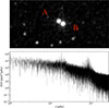 |
Fig. 1. Image of the AB KIC 8004637 from the Two Micron All Sky Survey in the JHKs bands (top panel) and its Fourier spectrum from Kepler data (bottom panel). Given the small spatial separation of these stars in the sky, their oscillations are detected in the same light curve. |
A theoretical binary population synthesis study by Miglio et al. (2014) predicted the presence of at least 200 ABs in the Kepler long-cadence dataset. The majority of these systems are expected to be composed of two core helium-burning (CHeB) red-clump stars, with orbital periods, Porb, ranging from 10 to 108 days. More recently, Mazzi et al. (2025) indicated that ABs are expected to exhibit a mass ratio close to 1 and are unlikely to interact (e.g. via mass transfer). Such interactions could hinder the detection of oscillations from both components, which favours a preserved initial semi-major axis.
Given that Kepler observed approximately 20 000 red giants in long-cadence mode, this prediction corresponds to an occurrence rate of roughly 1%, highlighting the rarity of such systems. Miglio et al. (2014) estimated a false-positive rate (i.e. spatially coincident but unassociated stars that appear within the 4-arcsecond Kepler pixel) of less than 10%. This implies that most of the detectable ABs should arise from genuine, gravitationally bound systems. Their detection is therefore particularly valuable, as it provides the opportunity to combine two independent techniques – asteroseismology and orbital dynamics – to infer and cross-validate stellar properties with high precision. Direct comparisons between seismic and dynamical estimates of stellar mass and radius make these systems fundamental benchmarks for testing and calibrating asteroseismic scaling relations. Although there are numerous binary systems in the Kepler field comprising at least one solar-like oscillator, only five confirmed gravitationally bound ABs have been reported to date (e.g. Appourchaux et al. 2015; Rawls et al. 2016; White et al. 2017; Beck et al. 2018; Li et al. 2018), all comprising main-sequence or sub-giant stars.
Asteroseismic binaries comprised by two CHeB stars are likely to have similar oscillation frequencies due to their narrow range in νmax. This similarity often results in them being seismically unresolved, complicating their detection. Choi et al. (2025) demonstrated that Shannon entropy, a concept from communication theory (Shannon 1948), can be used to identify these configurations. However, conducting a systematic search for thesesystems remains a challenge. In contrast, ABs comprising at least one red-giant branch (RGB) star are more likely to be seismically resolved, and thus easier to detect. Although they represent only a small fraction of the predicted AB population, they provide a valuable initial sample for testing predictions regarding binary populations.
In this study, we aim to identify ABs formed by gravitationally bound stars. Miglio et al. (2014) predicted that approximately 80% of the ABs should have orbital periods longer than 103 days. Such systems can therefore be expected to be formed by widely separated stars.
Wide binaries, also referred to as common proper motion pairs, are characterised by semi-major axes exceeding 100 AU and orbital periods ranging from 10 to 108 yr. Although easily resolvable on the sky, their wide separations make their detection susceptible to contamination from chance alignments; therefore, precise astrometric measurements are necessary to confirm gravitational binding. For this reason, we applied a detection method based on Kepler’s third law and Gaia data (including parallaxes, proper motions, and radial velocities) to analyse a sample of 40 Kepler targets whose Fourier spectra exhibit two distinct sets of solar-like oscillations within frequency ranges characteristic of red-giant stars. In particular, we followed the work of El-Badry et al. (2021), in which they constructed the largest catalogue of bona fide wide binaries from Gaia DR3 to date based on their observed total orbital velocity differences.
This paper is organised as follows. In Section 2, we describe the sample selection, and in Section 3 we present the asteroseismic analysis of Kepler light curves. We provide details on the cross-matching between Gaia DR3 and Kepler sources in Section 4, followed by the assessment of gravitational binding in Section 5. In Section 6 we discuss the binary likelihood of two wide binary candidates, KIC 10094545 and KIC 6501237, along with new candidates for spatially unresolved systems. Finally, we summarise our findings in Section 7.
2. Sample of asteroseismic binaries
Our sample comprises 44 ABs observed in Kepler long-cadence (Δt = 29.4 min) data. Of these, 27 systems were identified by Bell et al. (2019) using pre-processed light curves from KASOC2. These systems exhibit multiple power excesses within the same power density spectrum (PDS), and were detected via the coefficient of variation (CV) method. This method, specifically designed for long-cadence Kepler data, assumes that the PDS derived from the Lomb-Scargle periodogram of a Gaussian white noise time series follows a chi-squared distribution with two degrees of freedom ( ). Under this assumption, the CV – defined as the ratio of the standard deviation to the mean of the power – should equal 1. Any signal not attributable to stochastic noise, such as solar-like oscillations, will exhibit higher CV values.
The remaining 17 systems were identified serendipitously during the preparation of CAPASS (Catalogue of Asteroseismic Parameters for the Analysis of Stellar Structure, Espinoza-Rojas et al., in prep.), using light curves from KEPSEISMIC3 (García et al. 2011). These targets were initially flagged due to significant discrepancies between their νmax estimates derived in our work and those reported in the literature (e.g. Yu et al. 2018; Pinsonneault et al. 2018; Kallinger 2019). Upon inspection, these discrepancies were found to result from the presence of two solar-like oscillators. Although the CV method is not applicable to KEPSEISMIC data due to altered noise statistics introduced during the data reduction process (see García et al. 2011, 2014; Pires et al. 2015, for further details), these visually identified systems complement the KASOC sample.
There are five ABs detected in CAPASS that also have KASOC light curves. However, they were not reported by Bell et al. (2019). After revising these systems using the CV method, we confirmed the presence of two solar-like oscillators in KIC 7345204, KIC 7697607, and KIC 10094545. In the case of KIC 4663623, the star at lower frequencies is significantly affected by photometric dilution, which prevents it from meeting the detection threshold adopted by Bell et al. (2019), despite its oscillations being visible in the power density spectrum. Furthermore, the KASOC light curve of KIC 7966761 reveals only the low-frequency oscillator, whereas the higher-frequency companion is detectable exclusively in the KEPSEISMIC light curve. Accordingly, we used KASOC data for the first four ABs and KEPSEISMIC for the latter.
Finally, we identified four duplicated ABs, i.e. two Kepler targets exhibiting the same pair of oscillations: KIC 4663623/KIC 4663627, KIC 5024297/KIC 5024312, KIC 9893437/KIC 9893440, and KIC 11090673/KIC 11090674. After removing duplicates, our final sample consists of 40 unique seismically resolved ABs.
3. Asteroseismic analysis
The power density spectrum of a single red-giant star consists of a granulation background and a power excess hump produced by solar-like oscillations. In contrast, our sample of ABs exhibits a PDS with two distinct sets of oscillations, each well separated and confined to a different frequency range (see top panel of Fig. 2 as an example). To extract their global asteroseismic parameters, we used the data-driven code Tools for Automated Characterisation of Oscillations (TACO, Hekker et al., in prep.). Given the dual nature of our targets, we modified TACO to account for the presence of two power excesses in the PDS rather than just one. For clarity, throughout this paper we refer to the component with lower-frequency oscillations as the primary, or ‘star A’, and the higher-frequency component as the secondary, or ‘star B’.
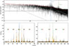 |
Fig. 2. Power density spectrum and peak-bagging results of KIC 6501237. In the top panel, the dotted blue and green lines indicate νmax, A and νmax, B, respectively. The four granulation components are represented by dashed grey lines, while the white noise is shown as a dash-dotted line. The total background model is depicted as a solid red line. The lower panels show the fitted oscillation modes of both solar-like oscillators in orange. Radial, quadrupole, and octupole modes are marked by red circles, green squares, and yellow hexagons. |
3.1. Background and νmax fit
We employed a modified version of the global fitting approach by Kallinger et al. (2014) to model the PDS. The model can be described by a superposition of granulation, Pgran, power excesses from stellar oscillations, Posc, of both stars, and a white noise term, Wnoise,
![Mathematical equation: $$ \begin{aligned} P(\nu ) = W_{\rm noise} + \eta ^{2}(\nu )[P_{\rm gran}(\nu ) + P_{\rm osc}], \end{aligned} $$](/articles/aa/full_html/2025/11/aa55884-25/aa55884-25-eq2.gif) (1)
(1)
where η = sinc(πν/2νNyq) is the apodisation accounting for discrete flux sampling, and νNyq is the Nyquist frequency.
The granulation background was modelled using a sum of s super-Lorentzian components:
 (2)
(2)
where Ai and bi are the characteristic amplitude and frequency, respectively. While two or three components are typically sufficient to characterise the granulation background, we used s = 4 to account for additional granulation noise introduced by the second star.
Each power excess hump was modelled as a Gaussian envelope centred on the respective frequency of maximum oscillation power, νmax, i,
 (3)
(3)
where Pg, i and σenv, i are the height and width of the Gaussian envelope of star i.
The fitting of the PDS model given by Eq. (1) was performed using an affine-invariant Markov chain Monte Carlo (MCMC) algorithm (Goodman & Weare 2010) implemented via the emcee Python package (Foreman-Mackey et al. 2013). This implies that the variables of the Gaussian envelope (i.e. νmax, Pg and σenv), granulation components (i.e. Ai, bi), and Wnoise are free parameters. We took the median values of the posterior distributions as our best-fit parameters, with uncertainties defined by their 16th and 84th percentiles. An example fit for KIC 6501237 is shown in Fig. 2, where the vertical dotted blue and green lines indicate the fitted νmax values of the two components, located at around 62.7 μHz and 122.5 μHz.
To normalise the PDS, we divided the power by the global model fit excluding the two Gaussian components, Posc, in Eq. (1) (see solid red line in Fig. 2). Subsequently, we extracted individual normalised PDS within the frequency range νmax ± 3σenv of each star. These background-normalised spectra were used for the remainder of the analysis.
3.2. Estimation of the large frequency separation, Δν
The identification of the spherical degree, ℓ, of each oscillation mode is essential for determining various asteroseismic parameters. In particular, radial modes (ℓ = 0) are used to estimate the large frequency separation, Δν, which is the spacing between consecutive overtones of the same degree. To estimate Δν, we performed a linear regression of the identified ℓ = 0 modes as a function of radial order to compute a global value of Δν, and assigned the standard error as uncertainty. Further details regarding this process and the mode identification of ℓ = 0, 2, and 3 are provided in Appendix A.2. The lower panels of Fig. 2 illustrate the peak fitting and mode identification results for both stars in KIC 6501237.
3.3. Fundamental stellar properties from scaling relations
Asteroseismic scaling relations were originally developed to predict the frequencies of the solar-like oscillators from spectroscopic atmospheric parameters (see Hekker 2020, for a review). Brown et al. (1991) empirically showed that νmax scales with the acoustic cut-off frequency νac, which represents a typical atmospheric dynamical timescale and is therefore proportional to the stellar surface gravity, g. This relation is commonly expressed as (Kjeldsen & Bedding 1995)
 (4)
(4)
 (5)
(5)
In addition, Kjeldsen & Bedding (1995) showed that Δν is proportional to the square root of the mean stellar density,  , based on the asymptotic approximation. This relation is also supported by detailed stellar models (Ulrich 1986), and can be expressed as
 (6)
(6)
Here ‘ref’ denotes reference values. Following Themeßl et al. (2018a), we used νmax, ref = 3166 ± 6 μHz, which is derived from various solar estimates, and Δνref = 130.8 ± 0.9 μHz to account for structural differences between the Sun and red-giant stars. We also adopted Teff, ⊙ = 5771.8 ± 0.7 K (Mamajek et al. 2015; Prša et al. 2016). By rearranging the above expressions, stellar mass and radius can be estimated with the following scaling relations:
 (7)
(7)
 (8)
(8)
Several studies have proposed refinements to these scaling relations to improve the accuracy of the stellar parameter determinations, accounting for deviations due to structural differences between red giants and the Sun, surface effects, and dependencies on metallicity or stellar mass (e.g. Sharma et al. 2016; Miglio et al. 2016; Pinsonneault et al. 2018; Themeßl et al. 2018a; Hekker 2020). In this work, we have applied corrections only through the use of the Δν reference value calibrated by Themeßl et al. (2018a), which incorporates mass, temperature, metallicity dependence, and surface effects. This calibration was shown to improve the agreement between asteroseismic and dynamical estimates of stellar parameters. Since our goal is to obtain only approximate estimates of stellar mass and radius, we consider this calibration to be sufficient and have not applied further adjustments to the scaling relations.
In addition to estimating fundamental parameters, we also used the scaling relations for their original purpose: predicting the oscillation frequencies of solar-like stars. This approach is especially useful given the relatively large pixel size of Kepler, which complicates the source matching of our sample of red giants with Gaia DR3. Asteroseismic parameters, particularly νmax, provide an additional constraint in this process. We defined  as the frequency of maximum oscillation power predicted from surface gravity and effective temperature (Eq. 4), and used it in our source-matching procedure (see Sect. 4.3).
4. Identification of asteroseismic binary members
Identifying Gaia DR3 counterparts to individual stars in ABs is challenging due to the limited spatial resolution of Kepler. Within a single target pixel file (TPF), multiple nearby stars can fall within the photometric aperture and potentially contribute their light to the structure which is visible in the PDS. We refer to these possible contributors as AB-member candidates, and we aim to identify which of them are the observed solar-like oscillators.
We used the interactive_sky function provided by the lightkurve package4 (Lightkurve Collaboration 2018) to extract the source_id of each candidate. This tool displays Gaia sources within the field of view of each Kepler TPF. Given the similarity between the GaiaG band and the KeplerKp band, we limited our selection to sources with 7 < phot_g_mean_mag < 17, ensuring sensitivity to the most likely contributors to the observed signal. This process yielded 101 AB-member candidates across our sample, with an average of 2.5 AB-member candidates per TPF.
4.1. Astrometric and spectroscopic parameters from surveys
We extracted astrometric and photometric parameters from Gaia DR3 for all AB-member candidates, including positions (α, δ), proper motions (μ), parallaxes (ϖ), G-band photometry, and, when available, radial velocities (Vr). To assess potential unresolved multiple systems, we also retrieved their re-normalised unit weight error (RUWE) values and non_single_star flags. A RUWE value of around 1.0 typically indicates that the astrometric solution is consistent with a single-star model, while values exceeding 1.4 (or 1.2 in less stringent cases, Castro-Ginard et al. 2024) suggest possible binarity (e.g. Lindegren et al. 2018; Belokurov et al. 2020; Penoyre et al. 2022; Castro-Ginard et al. 2024). The non_single_star flag further classifies stars as either (1) astrometric, (2) spectroscopic, or (3) eclipsing binaries (Halbwachs et al. 2023; Gosset et al. 2025). Among the 101 AB-member candidates, 11 exhibit high RUWE values, and two5 are classified as spectroscopic binaries based on their non_single_star flag. Furthermore, we inspected the phot_variable_class in Gaia DR3 to exclude classical pulsators (e.g. RR-Lyrae, δ Scuti, Cepheids), since their oscillations do not correspond to the signals observed in the PDS of any of the ABs in our sample.
To correct for known biases in Gaia parallaxes, we applied the zero-point corrections described by Lindegren et al. (2021a), using the publicly available gaiadr3_zeropoint package6. In addition, we followed the approach of El-Badry et al. (2021) to adjust the reported parallax uncertainties, accounting for underestimation in bright stars (11 < G < 13), close pairs, and sources with high RUWE values or poor Gaia image parameter diagnostics (e.g. ipd_gof_harmonic_amplitude > 0.1, ipd_frac_multi_peak > 10). The applied corrections have average values of ∼0.025 mas in parallax and ∼0.041 mas in parallax uncertainty. Furthermore, we retained only stars with good-quality astrometric data; that is, with parallax uncertainties of σϖ < 2 mas and parallax fractional uncertainties of ϖ/σϖ > 5 (e.g. El-Badry & Rix 2018; El-Badry et al. 2021).
In addition to the astrometry, we retrieved stellar atmospheric parameters derived from low-resolution BP/RP spectra from Gaia DR3 (GSP-Phot; Andrae et al. 2023), and from combined radial velocity spectra from GSP-Spec (Recio-Blanco et al. 2023). We also incorporated spectroscopic and photometric information from SDSS-IV/APOGEE DR16 (Abdurro’uf et al. 2022).
4.2. Removing main-sequence and white-dwarf stars
To restrict our sample of AB-member candidates to red-giant stars, we used the Gaia colour-magnitude diagram (CMD) to exclude sources located in the main-sequence and white dwarf regions. For this purpose, we adopted the Gaia CMD boundaries defined by Godoy-Rivera et al. (2025). Briefly, they used PARSEC (PAdova and tRiestet Stellar Evolutionary Code; Bressan et al. 2012; Chen et al. 2014; Nguyen et al. 2022) evolutionary tracks with solar metallicity to characterise different stellar populations, including the main sequence, subgiant and red giant branch, and white dwarfs. In addition, Godoy-Rivera et al. (2025) provides G-band absolute magnitudes (MG) and BP − RP colours corrected for extinction (AG) and reddening (E(BP − RP)), respectively, for all the stars in the Kepler-Gaia DR3 cross-match7.
Since many of our AB-member candidates are not part of the Kepler-Gaia catalogue, extinction and reddening estimates were unavailable for a large fraction of them. While GSP-Phot provides such values, its strong distance prior introduces systematic overestimates in Teff and log g (see Andrae et al. 2023). As an alternative, we adopted the mean extinction and reddening values of red giants in APOKASC 3 (Pinsonneault et al. 2025) that are part of the sample of Godoy-Rivera et al. (2025). We found average values of E(BP − RP)∼0.11 and AG ∼ 0.23. Rather than correcting each star, we applied a global shift to the red-giant region boundaries in the CMD. This adjusted region is shown as the light blue contour in Fig. 3. Since this filtering process requires an absolute magnitude estimate, AB-member candidates lacking Gaia photometry or parallax estimates were also excluded. As is discussed by Godoy-Rivera et al. (2025), restricting the composition of the models used to define the CMD region to solar metallicity can affect the final classification. They found that, at lower metallicities, the regions become redder and less luminous. However, they demonstrated that their classification method is robust against changes in metallicity of around ±0.2 dex. We consider their approach to be sufficiently accurate for the purposes of our study.
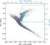 |
Fig. 3. Gaia colour-magnitude diagram of the AB-member candidates. Grey points represent Kepler stars from Godoy-Rivera et al. (2025), with extinction- and reddening-corrected photometry, plotted using the black axes. The light blue axes are used to plot the Gaia DR3 photometry of our sample that lacks E(BP − RP) and AG corrections. The light blue line depicts the borders of the giant-stars region defined by Godoy-Rivera et al. (2025), adjusted to account for the missing photometric corrections. AB-member candidates classified as giants according to this criterion are shown in cyan, while those excluded by the criteria are shown as blue circles. |
This filtering yielded a final sample of 71 red-giant AB-member candidates, shown as cyan circles in Fig. 3, which are used for the rest of the analysis. Given the small magnitude of the extinction and reddening corrections, we do not expect this approximation to significantly affect the results of our selection.
4.3. Matching asteroseismic and spectroscopic νmax values
For each red-giant AB-member candidate, we estimated the expected frequency of maximum oscillation power, denoted as  , using the relation
  , as described in Sect. 3.3. We prioritised spectroscopic atmospheric parameters from available surveys in the following order of spectral resolution and precision: APOGEE, GSP-Spec, and GSP-Phot.
Atmospheric parameters from GSP-Phot, particularly the effective temperature and surface gravity, are known to suffer from systematic biases. Andrae et al. (2023) report typical overestimations of approximately δTeff = 400 K and δlog g = 0.4 dex relative to APOGEE DR16, primarily due to strong distance priors based on d ∼ 1/ϖ. These biases are especially pronounced for stars with low-quality parallaxes (ϖ/σϖ < 20), which is common among distant red giants where the parallax-distance relation breaks down (see Bailer-Jones et al. 2021).
Among our red giant AB-member candidates, 20 stars have atmospheric parameters from GSP-Phot only. To mitigate the aforementioned biases, we applied empirical corrections following the values reported in Andrae et al. (2023). For stars with ϖ/σϖ ≤ 20, we subtracted the median absolute deviation (MAD) from the reported Teff; for log g, the MAD correction was applied only when ϖ/σϖ ≤ 10. For AB-member candidates with higher-quality parallaxes, we used the smaller MAD from the median (MedAD) values, which are considered more appropriate in the low-bias regime. The correction values were taken from Tables 1 and 2 of Andrae et al. (2023). Applying these corrections reduces  by 10−δlog g(1 − δTeff/Teff)−1/2 and reduces the seismic mass by (1 − δTeff/Teff)3/2. Additionally, we inflated the reported uncertainties by factors of 2.0 for Teff and 2.5 for log g to account for their underestimation, as recommended by Andrae et al. (2023). No corrections were applied to APOGEE (42 stars) or GSP-Spec (9 stars) parameters, as their calibrations are considered reliable within the context of this analysis.
To identify the most likely Gaia source for each red giant, we searched for candidates whose  fell within the range νmax ± 2Δν, also accounting for uncertainties in both parameters. Using this criterion, we successfully matched both solar-like oscillators to unique Gaia sources in 15 AB systems (see Table D.1). In 19 systems, we could confidently identify only one component (see Table D.2). Ten of these nineteen cases either lacked complete spectroscopic data for all AB-member candidates or did not have
  consistent with the asteroseismic estimates, i.e.
  is outside the search range (see central panel of Fig. D.1). Additionally, we found five of these nineteen systems to be associated with a single AB-member candidate that shows signs of being a non-single source (e.g. high RUWE), suggesting possible unresolved multiplicity. These systems are discussed in Sect. 6.3. In contrast, four other systems also have a single AB-member candidate and show no indication or multiplicity.
For the remaining six ABs, no match could be obtained for either star, since the estimated  did not fall within the search range, or there was only one AB-member candidate for the system, which in turn had a
  value between the two asteroseismic νmax estimates (bottom panel Fig. D.1). These cases are of particular interest and are further discussed in Sect. 6.4. Fig. 4 illustrates the differences in νmax and
  , with the colours representing the source of the atmospheric parameters. As was expected, spectroscopic estimates based on APOGEE data show better agreement with asteroseismic values than those from GSP-Phot or GSP-Spec.
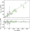 |
Fig. 4. Comparison of asteroseismic and spectroscopic νmax estimates of the Kepler-Gaia matched sources described in Sect. 4.3. Stars with atmospheric parameters from APOGEE, GSP-Spec, and GSP-Phot are shown in green, purple, and pink, respectively. Circles correspond to ABs where both solar-like oscillators of an AB were matched to a Gaia source. Squares depict ABs where only one of the two oscillators was matched. The bottom panel displays the difference in units of radial order, i.e. normalised by Δν. The dotted grey lines represent differences of ±1Δν. |
5. Finding gravitationally bound stars
Our sample of red-giant AB-member candidates includes, on average, two Gaia sources per Kepler target. We computed the angular separation, θ, using their Gaia positions:
 (9)
(9)
where αi and δi are the right ascension and declination, respectively. The subindex i = 1, 2 corresponds to the primary and secondary component, where, by definition, the primary is the brightest star of the pair. This convention differs from the asteroseismic designations star A and star B based on oscillation frequencies.
The angular separation can be converted into a projected physical separation, s, using a distance proxy from theirtrigonometric parallax, ϖ:
 (10)
(10)
We used the parallax of the brightest star in the pair as representative of the system. The smallest projected separations in our sample are larger than 1000 AU, suggesting that if any of these pairs are gravitationally bound, they are wide binaries. Accordingly, to assess the gravitational binding of our candidate pairs, we followed the approach implemented by El-Badry et al. (2021).
We required the parallaxes of the two stars in each pair to be consistent within uncertainty:
 (11)
(11)
Here, ϖ1 and ϖ2 are the parallaxes of the primary and secondary star, respectively, with σϖ1 and σϖ2 their corresponding uncertainties. As is discussed in El-Badry et al. (2021), the constant, b, is assigned a larger value at small separations to account for two reasons: (1) underestimated parallax uncertainties at close angular separations, and (2) a lower contamination rate from chance alignments in that regime.
The wider the binary system, the less likely it is to remain bound over long timescales, as its gravitational attraction weakens with increasing separation. This makes the widest binaries most susceptible to disruption by external perturbations, such as galactic tides and dynamical encounters in dense environments. Wide binaries are rarely found beyond projected separations of ∼1 pc (with a few exceptions, e.g. Chanamé & Gould 2004; Shaya & Olling 2011), corresponding to orbital periods of Porb ∼ 108 yr. As is discussed by Andrews et al. (2017), this limit reflects the scale at which the binding energy of the system becomes comparable to the Galactic tidal field given by the Milky Way Jacobi radius (Binney & Tremaine 2008). To avoid contamination by potentially unbound pairs, we applied the following constraint:
 (12)
(12)
which sets a maximum separation corresponding to s < 1 pc.
To test whether a given pair of stars is gravitationally bound, we required that their relative motions be consistent with Keplerian orbits. Under the assumption of circular orbits, the maximum total velocity difference expected for a binary according to Kepler’s third law is given by
 (13)
(13)
where a is the semi-major axis, and satisfies a ≥ s.
The total velocity difference of a binary is defined as the norm of the velocity difference vector:
 (14)
(14)
where ΔV⊥ is the tangential velocity difference and ΔVr = |Vr, 1 − Vr, 2|, i.e. the radial velocity difference. Then, any pair of stars that meets the condition ΔVtot < ΔVtot, max is classified as a binary system. However, radial velocities are not available for all the stars in our sample. Hence, if any of the components of a pair of stars lacks radial velocity measurements, we implement a different binary condition based exclusively on their tangential velocity difference (e.g. Andrews et al. 2017; El-Badry & Rix 2018; El-Badry et al. 2021; Barrientos & Chanamé 2021):
 (15)
(15)
Here, σΔV⊥ accounts for uncertainties in proper motion and parallax. Inflating the threshold by 3σ makes the criteria less conservative, but it can instead favour completeness by avoiding rejection of genuine binaries due to parallax and or proper motion noise, especially for distant stars. The tangential velocity difference is computed as
 (16)
(16)
 (17)
(17)
where Δμ and σΔμ are the total proper motion difference and its uncertainty, which are defined as
 (18)
(18)
 (19)
(19)
Here,  , and
, and  , where
  accounts for projection effects in right ascension.
In general, this method of detecting wide binaries assumes small angular separations (θ < 1°), where curvature effects in the sky-projected coordinates can be neglected. We find that all candidate pairs in our sample have separations of θ < 60 arcsec, confirming the validity of this approximation (see Fig. 5).
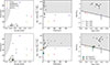 |
Fig. 5. Summary of binarity criteria. Top row: AB systems with both components successfully matched to Gaia sources (Table D.1). Bottom row: All possible pairs from AB-member candidate sets, excluding those in the top row. The left panels illustrate angular separation as a function of parallax, with limits from Eq. (12) (s < 1 pc) as a hatched grey region. The centre panels show parallax consistency; dashed black lines mark the criteria from Eq. (11). The right panels show the total orbital velocity difference versus projected separation (log-log scale), with theoretical ΔVtot values from Eq. (13) for Mtot = 3, 4, and 5 M⊙. Crosses, circles, and stars represent pairs that only satisfy one, two, or three binary conditions, respectively. Well-known bona fide wide binaries 16 Cygni, HD 80806/07, HIP 99727/29, and HAT-P-4 are shown as pink, orange, green, and purple diamonds, respectively. Genuine wide binary candidates are expected to lie within the white area of each plot. KIC 6501237 and KIC 10094545, highlighted as blue and orange stars, respectively, are identified as likely genuine wide binaries. |
Finally, we implemented a Monte Carlo approach to provide a probabilistic assessment of binarity accounting for uncertainties. For each pair, we generated 1000 realisations of the total velocity difference by sampling from a Gaussian distribution centred on ΔVtot and its corresponding uncertainty as the standard deviation. We then compared each realisation of ΔVtot with the theoretical velocity thresholds (see Eq. 13) computed for three different total masses: 3, 4, and 5 M⊙. This way, we estimated the probability of the observed motion being consistent with a bound system for each assumed total mass, yielding a set of three binary probability estimates per system. To account for biases produced by the sampling distribution selection, we repeated the same procedure using a uniform distribution centred in ΔVtot and with a width given by ±3σΔVtot.
6. Results
6.1. Wide binary candidates
The method described in Sect. 5 was applied to two different groups: (1) ABs in which both oscillating components were successfully matched to unique Gaia sources (see Table D.1), and (2) all other possible pairs of stars within each AB-member candidate list, excluding those in group 1. For the latter, we considered every unique pair combination, ensuring that no star was paired with itself and that no duplicated combinations were included. The results for group 1 and 2 are presented on the top and bottom row of Fig. 5, respectively.
For reference, Fig. 5 also includes four well-studied bona fide wide binaries: 16 Cygni (Tucci Maia et al. 2014), HD 80806/07 (Dommanget & Nys 2002; Mack et al. 2016), HIP 99727/29 (van den Bergh 1958; Ramírez et al. 2014), and HAT-P-4 (Mugrauer et al. 2014; Saffe et al. 2017). Each of these systems is formed by solar-type or solar-twin stars, with an estimated total mass of around 2 M⊙ (see Naef et al. 2001; Laughlin et al. 2009; Ramírez et al. 2014; Saffe et al. 2017; Bellinger et al. 2017) Using Gaia DR3 data, we re-computed their total velocity differences and confirmed their consistency with values previously reported in the literature (e.g. Ramírez et al. 2019). We also computed theoretical ΔVtot values assuming total system masses of 3, 4, and 5 M⊙, which are representative of red-giant binaries (see Pinsonneault et al. 2025). We find that this variation of ±1 M⊙ in the total mass has a minimal impact on our binary classification.
As illustrated in Fig. 5, none of the ABs in group 1 appear to be gravitationally bound, as their total velocity differences significantly exceed the theoretical thresholds, even when accounting for measurement uncertainties. These discrepancies are driven by large differences in parallax, proper motion, and/or radial velocity between the components. In contrast, we identified two systems from group 2, KIC 6501237 and KIC 10094545, with kinematics consistent with a wide binary scenario. For both systems, ΔVtot reaches values below the theoretical limits within 3σΔVtot according to the total mass of each system (2.74 M⊙ and 4.26 M⊙, respectively. See Table 1).
Spectroscopic, photometric, and asteroseismic parameters of the wide binary candidates in our sample.
It is worth noting that El-Badry et al. (2021) ensured the use of moderately precise astrometry by restricting their sample to stars with parallaxes greater than 1 mas, corresponding to distances of d ≲ 1 kpc. However, our analysis necessarily includes stars at larger distances, owing to the intrinsic brightness of red giants. As is discussed in Appendix C, this broader distance range pushes the method to regimes where the inverse parallax could no longer be a reliable proxy for distances. To evaluate the impact of this limitation, we re-calculated the total orbital velocity differences using geometric distances provided by Bailer-Jones et al. (2021) instead of 1/ϖ. We find that this substitution introduces negligible differences in the estimates of ΔVorb and does not change the conclusions of our analysis. For a more detailed discussion, we refer the reader to Appendix C.
6.1.1. KIC 10094545
The AB KIC 10094545 was identified by Bell et al. (2019) using the CV method. Its TPF contains only two AB-member candidates: Gaia DR3 2085575547024946048 (candidate A) and Gaia DR3 2085575547020615424 (candidate B). The stellar atmospheric parameters for candidate A were taken from APOGEE, while those for candidate B were sourced from GSP-Phot. As is discussed in Sect. 4.3, we applied corrections to the GSP-Phot values to address known systematic errors in distant stars.
Matching candidates A and B to the observed oscillations was challenging, as both candidates have spectroscopic νmax values within the uncertainties that agree with the value of 73 ± 1 μHz estimated for the primary star KIC 10094545A, i.e.  Hz and
  Hz. We solved this by selecting the candidate with the spectroscopic estimate closest to the asteroseismic estimate, i.e. candidate A was matched to star A. This choice is reliable given the precision of the stellar parameters from APOGEE of candidate A.
However, the value of  remained significantly offset from the asteroseismic νmax of star B, which is 122 μHz, even after applying corrections. These corrections resulted in an approximated decrease of 34 μHz in the estimated
  8. Since we prioritised APOGEE parameters due to their more reliable calibration, this suggests that the GSP-Phot values for candidate B can be affected by additional, uncorrected biases. Notably, the applied corrections shifted
  in the opposite direction relative to νmax, B, further supporting this interpretation. Consequently, we cannot confidently match the secondary star to any Gaia source in this system. Nonetheless, given the absence of other AB-member candidates in the TPF and the astrometric consistency of candidates A and B, we assume from this point forward that they correspond to the primary and secondary stars observed in KIC 10094545, respectively.
KIC 10094545 consists of a secondary clump (2CL) star and a RGB star (see Appendix B), with inferred seismic masses of MA = 2.52 ± 0.15 M⊙ and MB = 1.74 ± 0.08 M⊙, respectively (see Eq. 8). Proposed wide binary formation scenarios (e.g. Kouwenhoven et al. 2010; Tokovinin 2017) suggest that stars in such configurations are coeval and have similar chemical compositions (e.g. Tucci Maia et al. 2014; Ramírez et al. 2019; Hawkins et al. 2020; Espinoza-Rojas et al. 2021). This implies that binary stars with a mass ratio different from one could be found at different evolutionary stages once they have left the main sequence, as is the case of this AB. While these parameters (seismic mass estimates and evolutionary stages) alone are not enough to probe the wide binary nature of the system, they provide additional evidence supporting this scenario. However, the probability that this system is gravitationally bound, as defined in Sect. 5, is around 20% when compared to the theoretical orbital velocity difference of a 4 M⊙ system (as is shown by the orange line in Fig. 5). This probability increases to ∼25% for a total mass of 5 M⊙.
In summary, KIC 10094545 appears to be a promising wide binary candidate, based on the consistent asteroseismic masses and evolutionary stages of its components. However, our astrometric analysis indicates a probability of binarity of ∼20 − 25%, which prevents us from drawing a definitive conclusion. We encourage spectroscopic follow-up observations to better identify the secondary component and confirm binarity, for instance through radial velocity monitoring or elemental abundance analysis. To our knowledge, this is the first observational evidence supporting the binary nature of this system.
6.1.2. KIC 6501237
We successfully matched the secondary component, KIC 6501237B, to Gaia DR3 2104510919655573120 (hereafter candidate B) based on APOGEE atmospheric parameters. According to their relative astrometry, candidate B is likely part of a wide binary with Gaia DR3 2104510923954927104 (candidate A). However, the atmospheric parameters for candidate A – available only from GSP-Phot and after applying the corrections mentioned in Sect. 4.3 – yield  Hz, which is significantly higher than its asteroseismic value of νmax, A = 63 μHz. Similar to the case of KIC 10094545, this AB does not have other AB-member candidate and candidate B does not present any Gaia multiplicity indicators (i.e. high RUWE, non_single_star flag); therefore, we assume that candidate A corresponds to star A, and interpret the discrepancy between
  and νmax, A as large systematic biases in GSP-Phot parameters.
KIC 6501237 was first classified as a possible close to equal mass binary by Tayar et al. (2015) in the context of rapid rotation of low-mass red giants. Assuming that candidates A and B form a binary system with a mass ratio close to 1, we expect them to be in similar evolutionary phases. We find that both stars in this system are on the RGB (see Table 1). Furthermore, we estimated a seismic mass of 1.27 ± 0.05 M⊙ for candidate B using its atmospheric parameters from APOGEE. To estimate the mass of candidate A, we explored two approaches. First, we used its atmospheric parameters from GSP-Phot (MA, GSP − Phot). Second, we used the atmospheric parameters of candidate B as a proxy (MA, APOGEE). These approaches yielded mass estimates of MA, GSP − Phot = 1.77 ± 0.04 M⊙ and MA, APOGEE = 1.45 ± 0.04 M⊙. On the one hand, GSP-Phot parameters lead to a relatively large mass difference, mainly due to systematically overestimated effective temperatures and surface gravities. On the other hand, the APOGEE-based result suggests a smaller discrepancy, consistent with expectations for a binary system.
Our mass estimates are slightly higher than those reported by Tayar et al. (2015), MA = 1.31 M⊙ and MB = 1.39 M⊙, likely due to differences in νmax, Δν, and reference values. While Tayar et al. (2015) proposed coevality based on mass similarity, they rejected binarity due to photometric magnitude differences derived from UKIRT images. Although we were unable to confidently match the KIC 6501237A to a Gaia source, the evidence suggests that both candidates are part of a wide binary system. In particular, the asteroseismic masses are in good agreement, supporting a coeval origin for the two stars, and their relative astrometric motions of candidates A and B yield a binary probability of approximately 50%. As in the case of KIC 10094545, additional high-resolution spectroscopic observations are required to confirm the Gaia-Kepler cross-match and further establish the binary nature of the system.
6.2. KIC 2568888
We revisited KIC 2568888, an AB previously analysed in the study by Themessl et al. (2018b), which reported a low binary probability of only ∼0.1% based on a combined seismic and photometric analysis. We identified four AB-member candidates, of which only one passed the CMD-filtering criteria described in Sect. 4.2. This candidate9 exhibits a RUWE value of 1.5 and has a spectroscopic  μHz, derived from APOGEE DR17 stellar parameters, since no observations were available in APOGEE DR16, GSP-Phot, or GSP-Spec. While this candidate was not matched to either of the oscillating components, its
  lies between the two asteroseismic νmax values of the system (see Table D.3).
We note that this APOGEE target is flagged with STARFLAG=“PERSIST_HIG”, indicating that more than 20% of its pixels fall within the super-persistence regions of the APOGEE detectors. As is discussed in Holtzman et al. (2018), this effect is wavelength-dependent and can artificially enhance flux levels by over 10%, potentially distorting spectral features. We therefore suspect that the lack of a reliable match could be due to systematics introduced by super-persistence, which can further bias the derived atmospheric parameters.
KIC 2568888 remains an intriguing target for further study, particularly given its high RUWE value, which suggests that it is an unresolved binary system (e.g. Castro-Ginard et al. 2024). However, based on the current data, we are unable to confirm or discard its binary nature.
6.3. Gaia’s multiplicity indicators
Radial velocity variability can indicate the presence of a close companion or, in some cases, intrinsic stellar variability. In Table 2 we present a subset of seven stars that exhibit high RUWE values, implying potential multiplicity as is discussed in Sect. 4.1. To further investigate the likelihood of these stars forming a gravitationally bound system, we examined their radial velocity variation using Gaia DR3 indicators.
Red giants in ABs with high RUWE values (≳1.4).
Katz et al. (2023) provide two key variability indicators: rv_chisq_pvalue and rv_renormalised_gof. These are derived from the properties of the Gaia time series, and quantify the constancy and noise level of radial velocity measurements. Briefly, rv_chisq_pvalue is expected to be small for stars exhibiting significant radial velocity scatter, as is expected in binaries, while rv_renormalised_gof compares the observed scatter in radial velocity to the typical epoch uncertainty. The reliability of these indices improves for stars with at least ten transits (rv_nb_transits ≥ 10) and effective temperatures in the range of 3900 K < rv_template_teff < 8000 K. Following the classification criteria of Katz et al. (2023), stars with rv_chisq_pvalue ≤ 0.01 and rv_renormalised_gof > 4 are flagged as radial velocity variables. All stars in our sample have RV effective temperatures within the applicable range for this method.
Red giants in ABs with Gaia DR3 radial velocity variability indicators.
As is shown in Table 2, Gaia DR3 provides radial velocity variability indicators for only four of the seven stars in our sample. KIC 10841730 was studied in detail by Schimak et al. (in prep.), and was confirmed as a binary through long-term (> 4 years) radial velocity monitoring with the HERMES spectrograph (Raskin et al. 2011). The TPF of this system contains only one AB-member candidate, with a  of ∼51 μHz–located between the two asteroseismic estimates for star A and B (see Table D.3). As a result, the candidate was not matched to either component. This system thus serves as an illustrative example of an AB formed by a spatially unresolved binary system.
We find that KIC 5443536 has only one AB-member candidate, which exhibits the strongest evidence of radial velocity variability according to the criteria of Katz et al. (2023), closely resembling the case of KIC 10841730. The combination of these variability indicators together with its high RUWE value supports the interpretation of this system as a strong candidate of a spatially unresolved binary. Similarly, KIC 7729396A exhibits a rv_chisq_pvalue of 0.0001 and a rv_renormalised_gof of 2.73, indicative of significant radial velocity scatter, although these values do not fully meet the thresholds established by Katz et al. (2023). Taken together, these findings suggest that both systems are likely genuine binaries whose spatial components cannot be resolved in the current Gaia data, and are therefore compelling targets for future spectroscopic follow-up.
Furthermore, we identified five systems that, despite having a RUWE and other indicators consistent with a single-star solution, show highly significant radial velocity variability (see Table 3). The case of KIC 8479383 stands out among them, as we could not match any of the oscillations to its single AB-member candidate, similar to the cases mentioned above, KIC 10841730 and KIC 5443536.
6.4. Asteroseismic binaries with no Gaia DR3 match
As was mentioned in Sect. 4.3, there is a sub-sample of six systems for which neither component was matched to a Gaia source (see Table D.3). Three of these systems, KIC 2568888, KIC 8479383, and KIC 10841739, have already been discussed (Sects. 6.2 and 6.3). Here, we examine the remaining three cases and discuss their likelihood of being spatially unresolved binaries.
For KIC 7966761, which has only one AB-member candidate (candidate A), the absence of a match is attributed to the very low νmax of star A (2.76 ± 0.04 μHz) combined with the relatively small uncertainty in its spectroscopic estimate ( μHz) from GSP-Spec. Together, these factors result in a search range that is too narrow to allow any match. Upon re-examination of the TPF, we identified an additional Gaia source10, candidate A*, previously excluded from the AB-member candidates due to missing BP and RP magnitudes (see Sect. 4.2).
Candidate A* has an APOGEE-based spectroscopic estimate,  μHz, that closely matches the asteroseismic value of star A, making it the most plausible counterpart. Moreover, it exhibits significant multiplicity indicators: a RUWE of 2.08, rv_chisq_pvalue of 1.3 × 10⁻¹⁵, and rv_renormalised_gof of 35.9 (see Sect. 6.3). However, large discrepancies in parallax, radial velocity, and proper motion between candidates A and A* rule out any gravitational interaction between both stars. We suggest that the proximity of candidate A* may have biased the GSP-Spec parameter estimates for candidate A, thereby affecting
  and raising the possibility that it could correspond to star B instead. Given the strong multiplicity indicators for candidate A* and its lack of association with candidate A, its variability could arise from a companion that is likely not a red giant, as no third star is observed on the PDS of KIC 7966761. Explaining the origin of this AB remains a challenge and requires spectroscopic observations.
The only AB-member candidate of KIC 644149911 with a νmax value consistent with the RGB was excluded during the CMD-based filtering (Sect. 4.2) due to the absence of a parallax measurement. This Gaia source has a two-parameter solution (astrometric_params_solved= 3), indicating that only positions (α, δ) are available. Consequently, Gaia does not provide a RUWE value or any radial velocity variability indicators. As outlined in Sect. 4.4 of Lindegren et al. (2021b), such cases typically result from one or more astrometric parameters (or combinations thereof) being insufficiently constrained. Therefore, we are unable to draw any further conclusions regarding the nature of this AB.
KIC 9412408 resembles KIC 10841730 in that it presents only a single AB-member candidate whose  , based on APOGEE data, lies between the asteroseismic νmax values of the two components. However, this star has a RUWE value that indicates possible multiplicity. No further signs of activity or binarity have been found (see Gaulme et al. 2020).
Given that there are no additional AB-member candidates in the TPFs for these last two systems, we propose that the observed oscillations originate from spatially unresolved binaries, with the identified AB-member candidates corresponding to the primary components. Spectroscopic follow-up is needed to confirm this scenario.
Figure 6 summarises the final sample of ABs identified as likely gravitationally bound systems, based on wide binary probabilities, RUWE values, and radial velocity variability indicators. Asteroseismic binaries without effective temperature estimates for lack of a Gaia match are assigned a Teff of around 5200 − 5600 K.
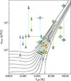 |
Fig. 6. Asteroseismic binaries likely to be gravitationally bound systems. Colours represent the method used to detect the binarity, where yellow, green, and light blue represent wide binaries (Table 1), stars with high RUWE (Table 2), and stars with RV variability indicators (Table 3), respectively. Circles represent ABs for which both solar-like oscillators were matched to a Gaia source (Table D.1). Squares depict ABs for which only one of the two oscillators was matched (Table D.2), and triangles correspond to ABs for which none of the oscillators was matched to a Gaia source (Table D.3). Black lines show Dartmouth evolutionary tracks (Dotter et al. 2008) for 0.8−2.6 M⊙ at solar metallicity, with mass decreasing from left to right. |
7. Summary and conclusions
Asteroseismic binaries offer a unique opportunity to detect binary systems with oscillating components and combine asteroseismology and orbital dynamics to constrain stellar properties. When gravitationally bound, these systems serve as valuable benchmarks for testing and calibrating asteroseismic scaling relations.
In this study, we have investigated the binarity of 40 seismically resolved ABs and used a modified version of the TACO pipeline (TACO, Hekker et al., in prep.) to extract global asteroseismic parameters and derive stellar masses and radii from scaling relations calibrated with updated reference values. For each AB, we identified AB-member candidates from Gaia DR3 sources located within their Kepler TPF. We filtered out main-sequence contaminants via CMD-based cuts using Gaia DR3 and cross-matched red giants with Gaia sources based on spectroscopic estimates of  derived from APOGEE, GSP-Spec, and GSP-Phot atmospheric parameters (the latter corrected for known systematics).
To assess whether AB-member candidates are gravitationally bound, we applied the wide binary detection method of El-Badry et al. (2021), using Gaia astrometry alone. For each pair, we computed projected separations and orbital velocity differences from parallaxes and proper motions, and compared them to theoretical expectations for Keplerian orbits. We then used Monte Carlo sampling to account for observational uncertainties and derived binary probabilities under different assumed total system masses.
The main findings of our study can be summarised as follows:
-
We identified two wide binary candidates – KIC 6501237 and KIC 10094545 – for which the astrometric properties are consistent with being gravitationally bound. Although only one of the two oscillating components in each AB was confidently matched to a Gaia DR3 source, the combination of their relative motions and asteroseismic mass estimates supports a common origin scenario. These systems have binary probabilities of ∼50% and ∼20%, respectively. They represent the most relevant cases of gravitationally bound ABs in our sample, and they are ideal targets for future spectroscopic confirmation.
-
Among the 15 ABs for which we confidently matched both oscillating components to Gaia sources, none show astrometric evidence of gravitational binding. This indicates that most of the ABs in our sample are likely chance alignments rather than true binary systems. However, it is important to note that our sample is limited to seismically resolved ABs, and this selection bias may influence our conclusions. To reconcile our findings with the predictions from Miglio et al. (2014), future studies should systematically search for ABs in Kepler long-cadence data, especially seismically unresolved systems, which Miglio et al. (2014) suggested are the most common type of AB.
-
For KIC 2568888, our astrometric analysis does not allow us to confirm or rule out binarity, primarily due to an incomplete Kepler-Gaia match. However, its only AB-member candidate has a high RUWE value (> 1.4), suggesting a possible unresolved companion. This system remains a promising target for future follow-up observations.
-
We examined Gaia multiplicity indicators (e.g. RUWE and radial velocity variability) for additional clues on binarity. These provided limited additional information. One of our targets, KIC 7729396, shows marginal signs of RV variability, yet we were not able to draw any firm conclusions about its multiplicity. In contrast, we found that the only AB-member candidate of KIC 5443536 is most likely a spatially unresolved multiple system. Furthermore, we found five additional cases that have highly significant radial velocity variability, despite presenting low RUWE estimates.
-
Only a single AB-member candidate was found on the TPFs of the systems KIC 6441499, KIC 8479383, and KIC 9412408. In all cases, the
 values were between the two asteroseismic νmax estimates. These systems resemble the case of KIC 10841730, which was confirmed as a binary in previous works. We propose that these can also be spatially unresolved binaries and encourage future spectroscopic follow-up.
We conclude that most ABs in our sample are likely chance alignments. However, two systems, KIC 6501237 and KIC 10094545, show astrometric and asteroseismic properties consistent with them being wide binaries. Furthermore, we propose KIC 2568888, KIC 5443536, KIC 6441499, KIC 8479383, and KIC 10841730 as spatially unresolved binary candidates. While these represent promising candidates, further spectroscopic follow-up is required to confirm their binarity and to refine the source identification. Such observations will be essential to fully assess their potential as benchmarks for stellar and asteroseismic studies.
The frequency of maximum oscillation power, νmax, scales with the acoustic cut-off frequency (Brown et al. 1991; Kjeldsen & Bedding 1995), which marks the transition point where acoustic waves are trapped in a cavity or become travelling waves.
Gaia DR3 2052444444184805376 and Gaia DR3 2075400563350022784.
The uncorrected value was  μHz.
μHz.
Gaia DR3 2051291674955780992.
Gaia DR3 2078200023020874240.
Gaia DR3 2101724344873978752.
Acknowledgments
We acknowledge funding from the ERC Consolidator Grant DipolarSound (grant agreement #101000296). This paper includes data collected by the Kepler mission and obtained from the MAST data archive at the Space Telescope Science Institute (STScI). Funding for the Kepler mission is provided by the NASA Science Mission Directorate. STScI is operated by the Association of Universities for Research in Astronomy, Inc., under NASA contract NAS 5-26555. This work has made use of data from the European Space Agency (ESA) mission Gaia (https://www.cosmos.esa.int/gaia), processed by the Gaia Data Processing and Analysis Consortium (DPAC, https://www.cosmos.esa.int/web/gaia/dpac/consortium). Funding for the DPAC has been provided by national institutions, in particular the institutions participating in the Gaia Multilateral Agreement.
References
- Abdurro’uf, Accetta, K., Aerts, C., et al. 2022, ApJS, 259, 35 [NASA ADS] [CrossRef] [Google Scholar]
- Aerts, C., Christensen-Dalsgaard, J., & Kurtz, D. W. 2010, Asteroseismology (Springer) [Google Scholar]
- Andersen, J. 1991, A&ARv, 3, 91 [Google Scholar]
- Andrae, R., Fouesneau, M., Sordo, R., et al. 2023, A&A, 674, A27 [CrossRef] [EDP Sciences] [Google Scholar]
- Andrews, J. J., Chanamé, J., & Agüeros, M. A. 2017, MNRAS, 472, 675 [NASA ADS] [CrossRef] [Google Scholar]
- Appourchaux, T., Antia, H. M., Ball, W., et al. 2015, A&A, 582, A25 [NASA ADS] [CrossRef] [EDP Sciences] [Google Scholar]
- Bailer-Jones, C. A. L. 2015, PASP, 127, 994 [Google Scholar]
- Bailer-Jones, C. A. L., Rybizki, J., Fouesneau, M., Demleitner, M., & Andrae, R. 2021, AJ, 161, 147 [Google Scholar]
- Barrientos, M., & Chanamé, J. 2021, ApJ, 923, 181 [NASA ADS] [CrossRef] [Google Scholar]
- Beck, P. G., Hambleton, K., Vos, J., et al. 2014, A&A, 564, A36 [NASA ADS] [CrossRef] [EDP Sciences] [Google Scholar]
- Beck, P. G., Hambleton, K., Vos, J., et al. 2015, Eur. Phys. J. Web Conf., 101, 06004 [CrossRef] [EDP Sciences] [Google Scholar]
- Beck, P. G., Kallinger, T., Pavlovski, K., et al. 2018, A&A, 612, A22 [NASA ADS] [CrossRef] [EDP Sciences] [Google Scholar]
- Beck, P. G., Mathur, S., Hambleton, K., et al. 2022, A&A, 667, A31 [NASA ADS] [CrossRef] [EDP Sciences] [Google Scholar]
- Bedding, T. R. 2014, in Asteroseismology, eds. P. L. Pallé, & C. Esteban, 60 [Google Scholar]
- Bedding, T. R., Mosser, B., Huber, D., et al. 2011, Nature, 471, 608 [Google Scholar]
- Bell, K. J., Hekker, S., & Kuszlewicz, J. S. 2019, MNRAS, 482, 616 [Google Scholar]
- Bellinger, E. P., Basu, S., Hekker, S., & Ball, W. H. 2017, ApJ, 851, 80 [NASA ADS] [CrossRef] [Google Scholar]
- Belokurov, V., Penoyre, Z., Oh, S., et al. 2020, MNRAS, 496, 1922 [Google Scholar]
- Benbakoura, M., Gaulme, P., McKeever, J., et al. 2021, A&A, 648, A113 [NASA ADS] [CrossRef] [EDP Sciences] [Google Scholar]
- Bétrisey, J., Buldgen, G., Reese, D. R., & Meynet, G. 2024, A&A, 681, A99 [NASA ADS] [CrossRef] [EDP Sciences] [Google Scholar]
- Binney, J., & Tremaine, S. 2008, Galactic Dynamics: Second Edition (Princeton: Princeton University Press) [Google Scholar]
- Borucki, W. J., Koch, D., Basri, G., et al. 2010, Science, 327, 977 [Google Scholar]
- Bressan, A., Marigo, P., Girardi, L., et al. 2012, MNRAS, 427, 127 [NASA ADS] [CrossRef] [Google Scholar]
- Brown, T. M., & Gilliland, R. L. 1994, ARA&A, 32, 37 [NASA ADS] [CrossRef] [Google Scholar]
- Brown, T. M., Gilliland, R. L., Noyes, R. W., & Ramsey, L. W. 1991, ApJ, 368, 599 [Google Scholar]
- Castro-Ginard, A., Penoyre, Z., Casey, A. R., et al. 2024, A&A, 688, A1 [NASA ADS] [CrossRef] [EDP Sciences] [Google Scholar]
- Chanamé, J., & Gould, A. 2004, ApJ, 601, 289 [CrossRef] [Google Scholar]
- Chen, Y., Girardi, L., Bressan, A., et al. 2014, MNRAS, 444, 2525 [Google Scholar]
- Choi, J. Y., Espinoza-Rojas, F., Coppée, Q., & Hekker, S. 2025, A&A, 699, A180 [NASA ADS] [CrossRef] [EDP Sciences] [Google Scholar]
- Christensen-Dalsgaard, J. 2004, Sol. Phys., 220, 137 [Google Scholar]
- Dommanget, J., & Nys, O. 2002, VizieR Online Data Catalog: I/274 [Google Scholar]
- Dotter, A., Chaboyer, B., Jevremović, D., et al. 2008, ApJS, 178, 89 [Google Scholar]
- El-Badry, K., & Rix, H.-W. 2018, MNRAS, 480, 4884 [Google Scholar]
- El-Badry, K., Rix, H.-W., & Heintz, T. M. 2021, MNRAS, 506, 2269 [NASA ADS] [CrossRef] [Google Scholar]
- Elsworth, Y., Hekker, S., Johnson, J. A., et al. 2019, MNRAS, 489, 4641 [NASA ADS] [CrossRef] [Google Scholar]
- Espinoza-Rojas, F., Chanamé, J., Jofré, P., & Casamiquela, L. 2021, ApJ, 920, 94 [NASA ADS] [CrossRef] [Google Scholar]
- Foreman-Mackey, D., Hogg, D. W., Lang, D., & Goodman, J. 2013, PASP, 125, 306 [Google Scholar]
- García Saravia Ortiz de Montellano, A., Hekker, S., & Themeßl, N. 2018, MNRAS, 476, 1470 [CrossRef] [Google Scholar]
- García, R. A., Hekker, S., Stello, D., et al. 2011, MNRAS, 414, L6 [NASA ADS] [CrossRef] [Google Scholar]
- García, R. A., Mathur, S., Pires, S., et al. 2014, A&A, 568, A10 [Google Scholar]
- Gaulme, P., McKeever, J., Rawls, M. L., et al. 2013, ApJ, 767, 82 [Google Scholar]
- Gaulme, P., Jackiewicz, J., Appourchaux, T., & Mosser, B. 2014, ApJ, 785, 5 [NASA ADS] [CrossRef] [Google Scholar]
- Gaulme, P., Jackiewicz, J., Spada, F., et al. 2020, A&A, 639, A63 [EDP Sciences] [Google Scholar]
- Godoy-Rivera, D., Mathur, S., García, R. A., et al. 2025, A&A, 696, A243 [Google Scholar]
- Goodman, J., & Weare, J. 2010, Commun. Appl. Math. Comput. Sci., 5, 65 [Google Scholar]
- Gosset, E., Damerdji, Y., Morel, T., et al. 2025, A&A, 693, A124 [NASA ADS] [CrossRef] [EDP Sciences] [Google Scholar]
- Halbwachs, J.-L., Pourbaix, D., Arenou, F., et al. 2023, A&A, 674, A9 [NASA ADS] [CrossRef] [EDP Sciences] [Google Scholar]
- Hawkins, K., Lucey, M., Ting, Y.-S., et al. 2020, MNRAS, 492, 1164 [NASA ADS] [CrossRef] [Google Scholar]
- Hekker, S. 2020, Front. Astron. Space Sci., 7, 3 [NASA ADS] [CrossRef] [Google Scholar]
- Hekker, S., Debosscher, J., Huber, D., et al. 2010, ApJ, 713, L187 [Google Scholar]
- Hekker, S., Basu, S., Stello, D., et al. 2011, A&A, 530, A100 [NASA ADS] [CrossRef] [EDP Sciences] [Google Scholar]
- Hełminiak, K. G., Konacki, M., Maehara, H., et al. 2019, MNRAS, 484, 451 [Google Scholar]
- Holtzman, J. A., Hasselquist, S., Shetrone, M., et al. 2018, AJ, 156, 125 [Google Scholar]
- Howell, S. B., Sobeck, C., Haas, M., et al. 2014, PASP, 126, 398 [Google Scholar]
- Huber, D., Bedding, T. R., Stello, D., et al. 2010, ApJ, 723, 1607 [NASA ADS] [CrossRef] [Google Scholar]
- Huber, D., Ireland, M. J., Bedding, T. R., et al. 2012, ApJ, 760, 32 [Google Scholar]
- Huber, D., Zinn, J., Bojsen-Hansen, M., et al. 2017, ApJ, 844, 102 [Google Scholar]
- Kallinger, T. 2019, ArXiv e-prints [arXiv:1906.09428] [Google Scholar]
- Kallinger, T., Hekker, S., Mosser, B., et al. 2012, A&A, 541, A51 [NASA ADS] [CrossRef] [EDP Sciences] [Google Scholar]
- Kallinger, T., De Ridder, J., Hekker, S., et al. 2014, A&A, 570, A41 [NASA ADS] [CrossRef] [EDP Sciences] [Google Scholar]
- Katz, D., Sartoretti, P., Guerrier, A., et al. 2023, A&A, 674, A5 [NASA ADS] [CrossRef] [EDP Sciences] [Google Scholar]
- Kjeldsen, H., & Bedding, T. R. 1995, A&A, 293, 87 [NASA ADS] [Google Scholar]
- Kouwenhoven, M. B. N., Goodwin, S. P., Parker, R. J., et al. 2010, MNRAS, 404, 1835 [NASA ADS] [Google Scholar]
- Laughlin, G., Deming, D., Langton, J., et al. 2009, Nature, 457, 562 [NASA ADS] [CrossRef] [Google Scholar]
- Li, Y., Bedding, T. R., Li, T., et al. 2018, MNRAS, 476, 470 [Google Scholar]
- Lightkurve Collaboration (Cardoso, J. V. D. M., et al.) 2018, Astrophysics Source Code Library [record ascl:1812.013] [Google Scholar]
- Lindegren, L., Hernández, J., Bombrun, A., et al. 2018, A&A, 616, A2 [NASA ADS] [CrossRef] [EDP Sciences] [Google Scholar]
- Lindegren, L., Bastian, U., Biermann, M., et al. 2021a, A&A, 649, A4 [EDP Sciences] [Google Scholar]
- Lindegren, L., Klioner, S. A., Hernández, J., et al. 2021b, A&A, 649, A2 [EDP Sciences] [Google Scholar]
- Mack, C. E., III, Stassun, K. G., Schuler, S. C., Hebb, L., & Pepper, J. A. 2016, ApJ, 818, 54 [NASA ADS] [CrossRef] [Google Scholar]
- Mamajek, E. E., Prsa, A., Torres, G., et al. 2015, ArXiv e-prints [arXiv:1510.07674] [Google Scholar]
- Mazzi, A., Thomsen, J. S., Miglio, A., et al. 2025, A&A, 699, A39 [NASA ADS] [CrossRef] [EDP Sciences] [Google Scholar]
- Miglio, A. 2012, Astrophys. Space Sci. Proc., 26, 11 [Google Scholar]
- Miglio, A., Chaplin, W. J., Farmer, R., et al. 2014, ApJ, 784, L3 [CrossRef] [Google Scholar]
- Miglio, A., Chaplin, W. J., Brogaard, K., et al. 2016, MNRAS, 461, 760 [NASA ADS] [CrossRef] [Google Scholar]
- Mosser, B., Barban, C., Montalbán, J., et al. 2011a, A&A, 532, A86 [NASA ADS] [CrossRef] [EDP Sciences] [Google Scholar]
- Mosser, B., Belkacem, K., Goupil, M. J., et al. 2011b, A&A, 525, L9 [CrossRef] [EDP Sciences] [Google Scholar]
- Mosser, B., Elsworth, Y., Hekker, S., et al. 2012, A&A, 537, A30 [NASA ADS] [CrossRef] [EDP Sciences] [Google Scholar]
- Mosser, B., Benomar, O., Belkacem, K., et al. 2014, A&A, 572, L5 [NASA ADS] [CrossRef] [EDP Sciences] [Google Scholar]
- Mosser, B., Vrard, M., Belkacem, K., Deheuvels, S., & Goupil, M. J. 2015, A&A, 584, A50 [NASA ADS] [CrossRef] [EDP Sciences] [Google Scholar]
- Mugrauer, M., Ginski, C., & Seeliger, M. 2014, MNRAS, 439, 1063 [Google Scholar]
- Naef, D., Latham, D. W., Mayor, M., et al. 2001, A&A, 375, L27 [NASA ADS] [CrossRef] [EDP Sciences] [Google Scholar]
- Nguyen, C. T., Costa, G., Girardi, L., et al. 2022, A&A, 665, A126 [NASA ADS] [CrossRef] [EDP Sciences] [Google Scholar]
- Penoyre, Z., Belokurov, V., & Evans, N. W. 2022, MNRAS, 513, 5270 [Google Scholar]
- Pinsonneault, M. H., Elsworth, Y. P., Tayar, J., et al. 2018, ApJS, 239, 32 [Google Scholar]
- Pinsonneault, M. H., Zinn, J. C., Tayar, J., et al. 2025, ApJS, 276, 69 [NASA ADS] [CrossRef] [Google Scholar]
- Pires, S., Mathur, S., García, R. A., et al. 2015, A&A, 574, A18 [NASA ADS] [CrossRef] [EDP Sciences] [Google Scholar]
- Pourbaix, D., Tokovinin, A. A., Batten, A. H., et al. 2004, A&A, 424, 727 [NASA ADS] [CrossRef] [EDP Sciences] [Google Scholar]
- Prša, A., Harmanec, P., Torres, G., et al. 2016, AJ, 152, 41 [Google Scholar]
- Ramírez, I., Meléndez, J., & Asplund, M. 2014, A&A, 561, A7 [NASA ADS] [CrossRef] [EDP Sciences] [Google Scholar]
- Ramírez, I., Khanal, S., Lichon, S. J., et al. 2019, MNRAS, 490, 2448 [CrossRef] [Google Scholar]
- Raskin, G., van Winckel, H., Hensberge, H., et al. 2011, A&A, 526, A69 [CrossRef] [EDP Sciences] [Google Scholar]
- Rawls, M. L., Gaulme, P., McKeever, J., et al. 2016, ApJ, 818, 108 [Google Scholar]
- Recio-Blanco, A., de Laverny, P., Palicio, P. A., et al. 2023, A&A, 674, A29 [NASA ADS] [CrossRef] [EDP Sciences] [Google Scholar]
- Ricker, G. R., Winn, J. N., Vanderspek, R., et al. 2014, SPIE Conf. Ser., 9143, 914320 [Google Scholar]
- Saffe, C., Jofré, E., Martioli, E., et al. 2017, A&A, 604, L4 [NASA ADS] [CrossRef] [EDP Sciences] [Google Scholar]
- Shannon, C. E. 1948, Bell Syst. Tech. J., 27, 379 [Google Scholar]
- Sharma, S., Stello, D., Bland-Hawthorn, J., Huber, D., & Bedding, T. R. 2016, ApJ, 822, 15 [Google Scholar]
- Shaya, E. J., & Olling, R. P. 2011, ApJS, 192, 2 [CrossRef] [Google Scholar]
- Tassoul, M. 1980, ApJS, 43, 469 [Google Scholar]
- Tayar, J., Ceillier, T., García-Hernández, D. A., et al. 2015, ApJ, 807, 82 [NASA ADS] [CrossRef] [Google Scholar]
- Themeßl, N., Hekker, S., Southworth, J., et al. 2018a, MNRAS, 478, 4669 [Google Scholar]
- Themessl, N., Hekker, S., Mints, A., et al. 2018b, ApJ, 868, 103 [NASA ADS] [CrossRef] [Google Scholar]
- Tokovinin, A. 2017, MNRAS, 468, 3461 [NASA ADS] [CrossRef] [Google Scholar]
- Torres, G., Andersen, J., & Giménez, A. 2010, A&ARv, 18, 67 [Google Scholar]
- Tucci Maia, M., Meléndez, J., & Ramírez, I. 2014, ApJ, 790, L25 [NASA ADS] [CrossRef] [Google Scholar]
- Ulrich, R. K. 1986, ApJ, 306, L37 [Google Scholar]
- van den Bergh, S. 1958, AJ, 63, 246 [CrossRef] [Google Scholar]
- Vrard, M., Mosser, B., & Samadi, R. 2016, A&A, 588, A87 [CrossRef] [EDP Sciences] [Google Scholar]
- Wang, Y., Li, T., Bi, S., Bedding, T. R., & Li, Y. 2023, ApJ, 953, 182 [NASA ADS] [CrossRef] [Google Scholar]
- Weiss, W. W., Rucinski, S. M., Moffat, A. F. J., et al. 2014, PASP, 126, 573 [Google Scholar]
- White, T. R., Huber, D., Maestro, V., et al. 2013, MNRAS, 433, 1262 [Google Scholar]
- White, T. R., Benomar, O., Silva Aguirre, V., et al. 2017, A&A, 601, A82 [NASA ADS] [CrossRef] [EDP Sciences] [Google Scholar]
- Yu, J., Huber, D., Bedding, T. R., et al. 2018, ApJS, 236, 42 [NASA ADS] [CrossRef] [Google Scholar]
Appendix A: Peakbagging and mode identification
In this section, we provide a brief overview of how the oscillation modes are detected, fitted, and assigned a spherical degree ℓ using the TACO pipeline. For a detailed description of the full methodology, we refer the reader to Hekker et al. in prep.
A.1. Peak detection
To detect significant peaks around νmax, A and νmax, B, TACO implements a Mexican hat wavelet filter following the method described by García Saravia Ortiz de Montellano et al. (2018). The resulting peaks are then fitted using two different functions, depending on their spectral resolution δν. Resolved peaks are fitted using a Lorentzian profile:
 (A.1)
(A.1)
where Hpeak, νpeak, and γpeak denote the height, central frequency, and half-width at half-maximum (HWHM) of the peak, respectively. Unresolved peaks, where γpeak ∼ δν, are modelled with a sinc-squared function:
 (A.2)
(A.2)
Peak parameters are then optimised using a two-step fitting process. First, TACO performs a global maximum likelihood fit using the parameters derived from the detection process as initial guess. Subsequently, each peak is fitted individually while keeping the rest of the model fixed, and the uncertainties are estimated from the diagonal elements of the inverse of the Hessian matrix.
A.2. Mode identification
TACO identifies the central radial mode closest to νmax by cross-correlating the observed PDS with the universal pattern of ℓ = 0 solar-like oscillations (Mosser et al. 2011a)
 (A.3)
(A.3)
where ϵp is the phase offset, α the curvature term, and nmax = νmax/Δν the radial order nearest to νmax. We used νmax from the background fit and Δν from the scaling relation of Hekker et al. (2011) as an initial estimate. Subsequently, TACO identifies radial modes at higher and lower radial orders based on this relation.
Using the frequencies of all the significant ℓ = 0 modes, TACO performs a linear regression to derive global estimates of the seismic parameters Δν, ϵp, and α, as well as central values, Δνc, ϵp, c, and αc from the three central radial modes.
Finally, TACO searches for quadrupole (ℓ = 2) and octupole (ℓ = 3) modes. These are identified as broad peaks near the expected frequency region, based on estimates of δν02 and δν03 from Huber et al. (2010) and Mosser et al. (2011b), respectively.
This version of TACO does not identify dipole modes (ℓ = 1), which often exhibit complex mixed-mode patterns in red giants. These modes result from coupling between pressure and gravity waves, leading to deviations from the regular frequency spacing found in pure pressure modes, i.e. radial modes. Their identification requires more sophisticated modelling. Here, all significant peaks not assigned to ℓ = 0, 2, and 3 are flagged as dipole-mode candidates.
Appendix B: Evolutionary stage determination
The evolutionary stage of red-giant stars can be determined from asteroseismic parameters. As shown by Kallinger et al. (2012), the structural differences between RGB and red clump (RC) stars affect parameters derived from pure pressure modes, i.e. ℓ = 0. In particular, the central estimates of the large frequency separation Δνc and phase offset ϵp, c are sensitive to these differences: core-helium burning stars typically exhibit lower values of ϵp, c than hydrogen-shell burning stars at the same Δνc, as illustrated in the top panel of Fig. B.1. As discussed in Kallinger et al. (2012), red clump stars have a narrow range in Δνc due to their common core mass at the helium flash, while secondary clump stars, which are more massive, ignite helium non-degeneratively, allowing for a range of core masses and Δνc values. However, there is a region in the Δνc − ϵp, c space where RGB and RC stars overlap, complicating their classification using this method alone.
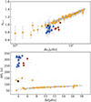 |
Fig. B.1. Evolutionary stages of our sample. Top: Phase shift of the three central radial modes, ϵc as a function of the central large frequency separation Δνc. Bottom: period spacing ΔΠ1 as a function of Δν. The stars are colour-coded by their evolutionary stage. Orange, blue, and red circles are RGB, red clump (RC), and secondary clump (2CL), respectively. A star with ambiguous evolutionary stage is shown as a black dot. The grey-background circles correspond to the “golden sample” from CAPASS (Espinoza-Rojas et al. in prep). |
In such cases, the presence of dipole mixed-modes is valuable, since they provide a more direct probe of the stellar core and hence the evolutionary stage. These modes exhibit a mixed character in red-giant stars, behaving as pressure-modes (p-modes) in the stellar envelope and as gravity-modes (g-modes) in the core due to coupling between the respective mode cavities (Bedding 2014). Mixed-modes follow a distinct pattern characterised by a near constant separation in period, also known as the period spacing ΔΠl (Tassoul 1980). This parameter carries indirect information about the core density and in dipole modes reaches values above 200 s for core-helium burning stars, while RGB stars show values between 50 and 100 s (e.g. Mosser et al. 2015; Vrard et al. 2016). This separation enables clear classification in the Δν − ΔΠ1 diagram (e.g. Bedding et al. 2011; Mosser et al. 2011a, 2012, 2014) (Fig. B.1, bottom panel).
We estimated ΔΠ1 by computing the Lomb-Scargle periodogram of the PDS without the ℓ = 0, 2 and 3 modes. However, our sample of stars are affected by photometric dilution, where flux blending from nearby sources in the same aperture reduces the observed oscillation amplitudes (e.g. Themeßl et al. 2018a), making the mode identification challenging and reducing the signal of modes with long lifetimes, i.e. narrow peaks. In such cases, the reliable estimation of ΔΠ1 is hampered. To mitigate this, we visually inspected the PDS to confirm whether the assigned evolutionary stage was consistent with the observed mode density, particularly the complex mode patterns expected in RC stars. The final evolutionary stages are shown in the lower panel of Fig. B.1.
As illustrated in Fig. B.1, one target remains ambiguous. Its position in both the Δνc − ϵp, c and Δν − ΔΠ1 diagrams lies between the RGB and RC regions. Similar cases have not been reported yet, but our analysis of single stars in CAPASS (Espinoza-Rojas et al. in prep) combined with evolutionary stages from Elsworth et al. (2019) suggest that both RGB and RC stars may appear in this region, and we cannot discard this arising from biases in the determination of ΔΠ1.
Appendix C: Limitations of wide binary detection for ϖ < 1 mas
As discussed in Bailer-Jones (2015), the use of inverse parallax as distance proxy (d ∼ 1/ϖ) is only reliable in the absence of noise. When the fractional parallax uncertainty exceeds 20% (σϖ/ϖ > 0.2), a probabilistic inference approach is required to obtain an unbiased estimate of distance. In this study, we applied quality cuts to exclude stars with large parallax uncertainties, thereby restricting our analysis to sources where the inverse-parallax remains valid as a proxy (dark grey points in Fig. C.1). To evaluate the impact of this assumption, we compared the inverse-parallax distances with those inferred by Bailer-Jones et al. (2021) from a probabilistic model.
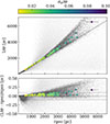 |
Fig. C.1. Comparison of Gaia DR3 inverse parallaxes as a function of geometric distances from Bailer-Jones et al. (2021). Dark grey background points represent a sample of 40000 randomly selected Gaia DR3 stars with fractional parallax error σϖ/ϖ < 0.2. Light grey points show stars with σϖ/ϖ > 0.2 from Bailer-Jones et al. (2021). Our sample of AB-member candidates are shown as circles, colour coded by their fractional parallax error. The bottom panel shows the respective residuals. Black dashed lines depict a difference of ±10%. |
As illustrated in Fig. C.1, the use of inverse parallax as a distance proxy is generally reliable for stars with good parallax quality, i.e. σϖ/ϖ < 0.2, up to distances of approximately 2 kpc. Beyond this range, the proxy tends to overestimate distances by ≥10%. The light grey background in Fig. C.1 represent stars with large fractional parallax uncertainties, illustrating that, without accounting for parallax quality, significant distance overestimations can arise already at ∼1 kpc. Consequently, the use of inverse parallax in the context of wide binary detection can introduce systematic errors in the derived projected separations and tangential velocity differences, potentially affecting the estimated binarity likelihood.
This limitation is particularly relevant for red-giant stars, which are intrinsically luminous and thus frequently observed at distances greater than 1 kpc. Careful consideration must therefore be given when applying the wide-binary detection method based on total orbital velocity differences to these stars, as the assumptions underlying the method can lead to ambiguous conclusions.
To quantify the impact of the inverse parallax distance prior on our binarity likelihood, we re-computed projected separations, tangential velocities and total orbital velocity differences for our whole set of AB-member candidates using the distances from Bailer-Jones et al. (2021). The equations presented in Sect. 5 were modified to use the distances instead of 1/ϖ. Hence, the projected separation becomes:
 (C.1)
(C.1)
whereas Eq. 12 can be expressed as:
 (C.2)
(C.2)
And finally, the tangential velocities can be rewritten as
 (C.3)
(C.3)
Note that the parallax consistency condition (Eq. 11) cannot be straightforwardly reformulated in terms of distance, as the interpretation of the uncertainty in parallax does not translate directly to distance space. The purpose of this exercise is merely to assess how the orbital velocities change when geometric distance estimates are used, rather than to redefine the consistency criterion. A full derivation of a revised distance-based condition is beyond the scope of this work. Furthermore, replacing inverse parallaxes with distance estimates from Bailer-Jones et al. (2021) leads to an increase in the uncertainties of the orbital velocity differences. For this reason, we do not report these revised values as final results.
As is shown in Fig. C.2, the resulting changes in binarity likelihood are negligible and do not affect the conclusions presented in Fig. 5 or the main finding of this study.
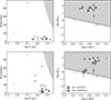 |
Fig. C.2. Same as left and right columns of Fig. 5, now using geometric distances from Bailer-Jones et al. (2021) instead of inverse parallaxes for the computation of projected separations and orbital velocities. |
Appendix D: Kepler-Gaia cross-match results
In this section, we summarise the cross-match between Kepler ABs and Gaia DR3 sources described in Sect. 4. The tables list seismic parameters, evolutionary stages, and Gaia multiplicity indicators (NSS solutions and RUWE) for three cases: both stars matched, one star matched, or no match. Figure D.1 illustrates these cases and compares seismic and spectroscopic νmax estimates.
D.1. Tables
List of asteroseismic parameters for systems where both solar-like oscillators were identified and matched to a Gaia DR3 source.
Asteroseismic parameters for systems which only one of the two solar-like oscillators was identified and matched to a Gaia DR3 source.
Asteroseismic parameters for systems in which neither of the two solar-like oscillators was matched to a Gaia DR3 source.
D.2. Figures
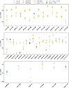 |
Fig. D.1. Results of matching Kepler ABs with Gaia DR3 sources. Top, centre and bottom panels show the ABs were both, only one and none of oscillators were matched Gaia source(s), respectively (see Tables D.1, D.2, and D.3). Grey up and down triangles indicate the asteroseismic νmax estimates. Diamonds, and right and left triangles represent spectroscopic νmax estimates derived from APOGEE, GSP-Spec and GSP-Phot stellar parameters, respectively. Stars with no indication of being unresolved multiple systems (RUWE < 1.2) are shown yellow, while stars with larger RUWE values are shown in green and purple. The only AB-member candidate of KIC 6441499 was excluded from the selection of red-giant stars due to the lack of Gaia photometry; therefore it is not shown in this plot (see Sect. 6.4). |
All Tables
Spectroscopic, photometric, and asteroseismic parameters of the wide binary candidates in our sample.
List of asteroseismic parameters for systems where both solar-like oscillators were identified and matched to a Gaia DR3 source.
Asteroseismic parameters for systems which only one of the two solar-like oscillators was identified and matched to a Gaia DR3 source.
Asteroseismic parameters for systems in which neither of the two solar-like oscillators was matched to a Gaia DR3 source.
All Figures
|
Fig. 1. Image of the AB KIC 8004637 from the Two Micron All Sky Survey in the JHKs bands (top panel) and its Fourier spectrum from Kepler data (bottom panel). Given the small spatial separation of these stars in the sky, their oscillations are detected in the same light curve. |
| In the text | |
|
Fig. 2. Power density spectrum and peak-bagging results of KIC 6501237. In the top panel, the dotted blue and green lines indicate νmax, A and νmax, B, respectively. The four granulation components are represented by dashed grey lines, while the white noise is shown as a dash-dotted line. The total background model is depicted as a solid red line. The lower panels show the fitted oscillation modes of both solar-like oscillators in orange. Radial, quadrupole, and octupole modes are marked by red circles, green squares, and yellow hexagons. |
| In the text | |
|
Fig. 3. Gaia colour-magnitude diagram of the AB-member candidates. Grey points represent Kepler stars from Godoy-Rivera et al. (2025), with extinction- and reddening-corrected photometry, plotted using the black axes. The light blue axes are used to plot the Gaia DR3 photometry of our sample that lacks E(BP − RP) and AG corrections. The light blue line depicts the borders of the giant-stars region defined by Godoy-Rivera et al. (2025), adjusted to account for the missing photometric corrections. AB-member candidates classified as giants according to this criterion are shown in cyan, while those excluded by the criteria are shown as blue circles. |
| In the text | |
|
Fig. 4. Comparison of asteroseismic and spectroscopic νmax estimates of the Kepler-Gaia matched sources described in Sect. 4.3. Stars with atmospheric parameters from APOGEE, GSP-Spec, and GSP-Phot are shown in green, purple, and pink, respectively. Circles correspond to ABs where both solar-like oscillators of an AB were matched to a Gaia source. Squares depict ABs where only one of the two oscillators was matched. The bottom panel displays the difference in units of radial order, i.e. normalised by Δν. The dotted grey lines represent differences of ±1Δν. |
| In the text | |
|
Fig. 5. Summary of binarity criteria. Top row: AB systems with both components successfully matched to Gaia sources (Table D.1). Bottom row: All possible pairs from AB-member candidate sets, excluding those in the top row. The left panels illustrate angular separation as a function of parallax, with limits from Eq. (12) (s < 1 pc) as a hatched grey region. The centre panels show parallax consistency; dashed black lines mark the criteria from Eq. (11). The right panels show the total orbital velocity difference versus projected separation (log-log scale), with theoretical ΔVtot values from Eq. (13) for Mtot = 3, 4, and 5 M⊙. Crosses, circles, and stars represent pairs that only satisfy one, two, or three binary conditions, respectively. Well-known bona fide wide binaries 16 Cygni, HD 80806/07, HIP 99727/29, and HAT-P-4 are shown as pink, orange, green, and purple diamonds, respectively. Genuine wide binary candidates are expected to lie within the white area of each plot. KIC 6501237 and KIC 10094545, highlighted as blue and orange stars, respectively, are identified as likely genuine wide binaries. |
| In the text | |
|
Fig. 6. Asteroseismic binaries likely to be gravitationally bound systems. Colours represent the method used to detect the binarity, where yellow, green, and light blue represent wide binaries (Table 1), stars with high RUWE (Table 2), and stars with RV variability indicators (Table 3), respectively. Circles represent ABs for which both solar-like oscillators were matched to a Gaia source (Table D.1). Squares depict ABs for which only one of the two oscillators was matched (Table D.2), and triangles correspond to ABs for which none of the oscillators was matched to a Gaia source (Table D.3). Black lines show Dartmouth evolutionary tracks (Dotter et al. 2008) for 0.8−2.6 M⊙ at solar metallicity, with mass decreasing from left to right. |
| In the text | |
|
Fig. B.1. Evolutionary stages of our sample. Top: Phase shift of the three central radial modes, ϵc as a function of the central large frequency separation Δνc. Bottom: period spacing ΔΠ1 as a function of Δν. The stars are colour-coded by their evolutionary stage. Orange, blue, and red circles are RGB, red clump (RC), and secondary clump (2CL), respectively. A star with ambiguous evolutionary stage is shown as a black dot. The grey-background circles correspond to the “golden sample” from CAPASS (Espinoza-Rojas et al. in prep). |
| In the text | |
|
Fig. C.1. Comparison of Gaia DR3 inverse parallaxes as a function of geometric distances from Bailer-Jones et al. (2021). Dark grey background points represent a sample of 40000 randomly selected Gaia DR3 stars with fractional parallax error σϖ/ϖ < 0.2. Light grey points show stars with σϖ/ϖ > 0.2 from Bailer-Jones et al. (2021). Our sample of AB-member candidates are shown as circles, colour coded by their fractional parallax error. The bottom panel shows the respective residuals. Black dashed lines depict a difference of ±10%. |
| In the text | |
|
Fig. C.2. Same as left and right columns of Fig. 5, now using geometric distances from Bailer-Jones et al. (2021) instead of inverse parallaxes for the computation of projected separations and orbital velocities. |
| In the text | |
|
Fig. D.1. Results of matching Kepler ABs with Gaia DR3 sources. Top, centre and bottom panels show the ABs were both, only one and none of oscillators were matched Gaia source(s), respectively (see Tables D.1, D.2, and D.3). Grey up and down triangles indicate the asteroseismic νmax estimates. Diamonds, and right and left triangles represent spectroscopic νmax estimates derived from APOGEE, GSP-Spec and GSP-Phot stellar parameters, respectively. Stars with no indication of being unresolved multiple systems (RUWE < 1.2) are shown yellow, while stars with larger RUWE values are shown in green and purple. The only AB-member candidate of KIC 6441499 was excluded from the selection of red-giant stars due to the lack of Gaia photometry; therefore it is not shown in this plot (see Sect. 6.4). |
| In the text | |
Current usage metrics show cumulative count of Article Views (full-text article views including HTML views, PDF and ePub downloads, according to the available data) and Abstracts Views on Vision4Press platform.
Data correspond to usage on the plateform after 2015. The current usage metrics is available 48-96 hours after online publication and is updated daily on week days.
Initial download of the metrics may take a while.